Optimization of Dense Medium Cyclone Plant for the...

Optimization of Dense Medium Cyclone Plant for the Beneficiation of Low Grade Iron Ore with Associated High Proportion of Near-Density Material at Sishen

Iron Ore Mine

by

Phakamile Tom (9110806D)

Report submitted to the Faculty of Engineering and the Built Environment, University of the

Witwatersrand, Johannesburg in partial fulfilment for the degree of Master of Science in

Engineering (Metallurgy and Materials Engineering)

Supervisor(s): Dr Murray M Bwalya

July 2015

6015768

Typewritten Text

08

i

DECLARATION

I declare that, apart from the acknowledged sources and assistance, this research report for the

Master of Science in Engineering (Metallurgy and Materials) degree to the School of Chemical

and Metallurgical Engineering, Faculty of Engineering and the Built Environment at the

University of the Witwatersrand is my own work and has not been submitted by me or another

person for a degree at this university or another institution of higher education.

Phakamile Tom

July 2015

6015768

Typewritten Text

08

ii

ABSTRACT

The research report is premised on three aspects which are critical in the heavy mineral

beneficiation. These aspects are classified as (i) understanding the densimetric profile of the

available ore body, (ii) understanding the properties of the heavy medium utilised at the plant to

beneficiate the ore, and (iii) the automation and modelling of the processing plant in order to

maximise plant efficiency.

Ore characterisation is mainly focused on understanding the densimetric profile of the ore body,

in order to determine the probability of producing a saleable product as well as predicting the

expected yields and quality. This is done to utilise the endowment entrusted upon the operating

entity by the government and shareholders to treat the mineral resource to its full potential.

Understanding of the beneficiation potential of the ore body will assist the mine planning and

processing plant to optimise the product tons and quality. This will ensure the marketing plans

are in accordance with the expected product as beneficiation will vary depending on the mining

block reserves. The mining blocks have potential to produce varying product grades with

different recoveries.

Ore characterisation was conducted on the GR80 mining block, low-grade stockpiles (i.e. C-

grade ore reserves & Jig discard and dense medium separation (DMS) run-of-mine (ROM)

material. The GR80 material was characterised as having low proportion of near-density

material and would be easy to beneficiate as well as produce high volumes of high grade

product. Furthermore, it was revealed that the 2014 DMS ROM had an increased proportion of

low-density material; however this material also had low proportion of near-density material.

The low-grade stockpiles was characterised by high proportion of near density material, which

necessitate the beneficiation process to operate at high density in excess of 3.8 t/m3.

Maintaining a higher operating density requires more dense medium which leads to viscosity

problems and impact performance.

The characterisation of the FeSi medium was imperative to understand its behaviour and

potential influence on beneficiation of low-grade stockpiles and mining blocks with elevated

proportion of near-density material. As the proportion of near-density waste material increases

in the run-of-mine (ROM), it is necessary to beneficiate the material at elevated operating

medium densities. However, when cyclones are operated at high densities, the negative

influence of the medium viscosity becomes more apparent and thus influences the separation

efficiency.

Heavy medium, ferrosilicon (FeSi) characterisation looked at identifying the effects of viscosity

iii

on the FeSi stability and whether there would be a need for a viscosity modifier. Thus, the

importance of controlling the stability, viscosity, and density of the medium cannot be under-

estimated and can very often override the improvements attainable through better designs of

cyclones. Furthermore, the slurry mixture of the heavy medium utilised for the purpose of dense

medium separation should be non-detrimental to the effectiveness of separation in the DMS

Fine cyclone plant. Medium characterisation showed that removal of ultra-fines leads to

unstable media as indicated by faster settling rates. This would result in medium segregation in

the beneficiation cyclone thereby leading to unacceptable high density differential which will

negatively impact the cut-point shift and cause high yield losses to waste.

The overall control of the metallurgical processes at Sishen’s Cyclone Plant is still done

manually and thus operation still varies from person-to-person and/or from shift-to-shift. This

result in some of the process data and trends not being available online as well as being

captured inaccurately. Furthermore, this negatively affects the traceability and reproducibility of

the production metallurgical key performance indicators (KPI’s) as well as process stability and

efficiency.

It has been demonstrated that real-time online measurements are crucial to maintaining

processing plant stability and efficiency thereby ensuring that the final product grade and its

value is not eroded. Modelling and automation of the key metallurgical parameters for the

cyclone plant circuit was achieved by installation of appropriate instrumentation and interlocking

to the programmable logic control (PLC). This allowed for the control of the correct medium

sump level, cyclone inlet pressure, medium-to-ore ratio as well as online monitoring of density

differential as “proxy” for medium rheological characteristics.

The benefit of modelling and simulation allows the virtual investigation and optimisation of the

processing plant efficiency as well as analysis of the impact of varying ore characteristics,

throughput variations and changing operating parameters. Due to the high tonnage for the iron

ore cyclone plant a modest increase in plant efficiency such as 1.5% yield increase would have

a large impact on plant profitability. Therefore it is imperative that all cyclone operating modules

are operated at the same efficiency which can be achieved by optimized process through proper

automation and monitoring, thereby improving the total plant profitability.

iv

ACKNOWLEDGEMENT

I would like to express my deepest appreciation to my MSc Eng. supervisor, Dr Mulenga

Bwalya, for guiding me in applying my undergraduate knowledge and improving my modelling

and simulation skills. This work would not be possible without his intelligent guidance and

extraordinary inspiration.

It is my pleasure to thank the plant management of Sishen Mine for entrusting me with

managing the optimisation and automation of the DMS cyclone plant. I would also like to thank

my sub-ordinates who took my instruction in taking process control samples and ensuring that

are delivered to respective laboratories for characterisation and conducting some process

monitoring in support of my project.

Special thanks go to my young brother, Zweli Tom, “an education enthusiast”, for his

encouragement and support which have always been a source of inspiration in my work and for

lending me his ears in time of doubt.

I would also like to express my sincere appreciation and thanks to my wife, Fikile and dedicate

this research report to my precious children Monwabisi, Thobekile, Keabetswe and Sthembiso.

v

TABLE OF CONTENTS

DECLARATION ........................................................................................................................... I

ABSTRACT ................................................................................................................................ II

ACKNOWLEDGEMENT ........................................................................................................... IV

TABLE OF CONTENTS ............................................................................................................ V

LIST OF FIGURES ................................................................................................................. VIII

LIST OF TABLES .................................................................................................................... XII

ACRONYMS AND DEFINITIONS ........................................................................................... XIII

ACRONYMS ........................................................................................................................... XIII

DEFINITION OF TERMS ............................................................................................................ XIII

CHAPTER 1: INTRODUCTION ............................................................................................. - 1 -

1 BACKGROUND ............................................................................................................. - 1 -

1.1 SISHEN DMS CYCLONE PLANT CIRCUIT ......................................................................... - 2 -

1.2 PROBLEM STATEMENT ................................................................................................... - 5 -

1.3 RESEARCH OBJECTIVE(S): ............................................................................................. - 6 -

CHAPTER 2: LITERATURE SURVEY .................................................................................. - 8 -

2 LITERATURE REVIEW ................................................................................................. - 8 -

2.1 WHAT IS DENSE MEDIUM SEPARATION ........................................................................... - 8 -

2.2 THEORY OF DENSE MEDIUM SEPARATION IN CYCLONE .................................................... - 8 -

2.2.1 Factors Influencing Dense Medium Beneficiation ............................................. - 11 -

2.2.2 Importance of Dense Medium Rheological Characteristics ............................... - 13 -

2.2.3 Cyclone Performance Measure......................................................................... - 16 -

2.2.4 Online Measurement, Control and Modelling .................................................... - 19 -

CHAPTER 3: METHODOLOGY .......................................................................................... - 25 -

3 EXPERIMENTAL APPROACH .................................................................................... - 25 -

3.1 ORE CHARACTERIZATION ............................................................................................ - 25 -

3.2 PROCESS FESI CHARACTERIZATION ............................................................................. - 25 -

3.2.1 Coarse FeSi Less Fines ................................................................................... - 28 -

3.2.2 Process FeSi .................................................................................................... - 28 -

3.2.3 Process FeSi Less Fines .................................................................................. - 29 -

vi

3.2.4 Viscosity Modifier .............................................................................................. - 29 -

3.3 PILOT TESTING OF AUTOMATED CYCLONE MODULE ...................................................... - 29 -

CHAPTER 4: ORE AND FESI CHARACTERISATION........................................................ - 35 -

4 ORE AND FESI CHARACTERISATION RESULTS..................................................... - 35 -

4.1 ORE CHARACTERISATION INTRODUCTION ..................................................................... - 35 -

4.1.1 Ore Densimetric and Chemical Analysis ........................................................... - 35 -

4.1.2 Characterisation Results of DMS Head Grade ROM Composite Samples ........ - 35 -

4.1.2.1 Impact of cut-density versus Ep ................................................................ - 37 -

4.1.3 Ore Characterisation Results of GR80 Mining Area Ore body .......................... - 40 -

4.1.4 Interpretation of Data for Samples from the Low Grade Stockpiles ................... - 44 -

4.1.5 Interpretation of Data for Samples from the Actual Pilot Plant Processing ........ - 47 -

4.1.6 Summary of Ore Characterisation and Processing Results ............................... - 51 -

4.2 FESI CHARACTERISATION INTRODUCTION ..................................................................... - 52 -

4.2.1 FeSi Rheology Test Results ............................................................................. - 52 -

4.2.2 Effect of Viscosity on FeSi Stability ................................................................... - 54 -

4.2.3 Material Property Test Results .......................................................................... - 54 -

4.2.4 Solids Density Results ...................................................................................... - 54 -

4.2.5 Particle Size Analysis ....................................................................................... - 55 -

4.2.6 FeSi Stability Tests ........................................................................................... - 56 -

4.2.6.1 Stability Test No 1: Static Settling Test Results ......................................... - 57 -

4.2.6.2 Stability Test No 2: Vertical Pipe Settling Tests ......................................... - 59 -

4.2.7 Comparison of Static and Vertical Pipe Settling Test Results ........................... - 62 -

4.2.8 Tube Viscometer Test Results .......................................................................... - 63 -

4.2.9 Summary of FeSi Characterisation Tests Results ............................................. - 67 -

CHAPTER 5: CYCLONE PLANT AUTOMATION AND CONTROL .................................... - 69 -

5 AUTOMATION AND CONTROL INTRODUCTION ...................................................... - 69 -

5.1 AUTOMATED MODULE VERSUS TRADITIONAL MODULE ................................................... - 72 -

5.2 MODULE 811 PERFORMANCE TRENDS ......................................................................... - 74 -

5.2.1 Monitoring and Control of Medium-to-Ore Ratio ................................................ - 75 -

5.2.2 Monitoring and Control of Cyclone Inlet Pressure ............................................. - 77 -

5.2.3 Monitoring and Control of Density Differential Measurement ............................ - 81 -

vii

CHAPTER 6: MODELLING OF DENSE MEDIUM CYCLONE CIRCUIT ............................. - 84 -

6 DENSE MEDIUM CYCLONE MODELLING INTRODUCTION ..................................... - 84 -

6.1 CORRECT MEDIUM SUMP LEVEL MODELLING ................................................................ - 85 -

6.2 CYCLONE PERFORMANCE MODELLING ......................................................................... - 89 -

CHAPTER 7: CONCLUSIONS AND RECOMMENDATIONS .............................................. - 96 -

7 CONCLUSIONS AND RECOMMENDATIONS ............................................................ - 96 -

7.1 CONCLUSIONS ............................................................................................................ - 96 -

7.1.1 Ore and FeSi Characterisation Conclusions ..................................................... - 96 -

7.1.2 Automation and Modelling Conclusions ............................................................ - 97 -

7.2 RECOMMENDATIONS FOR FUTURE WORK ...................................................................... - 98 -

REFERENCES AND APPENDICES .................................................................................... - 99 -

REFERENCES .................................................................................................................... - 99 -

APPENDICES ................................................................................................................... - 102 -

APPENDIX A: ORE CHARACTERISATION .................................................................... - 102 -

7.2.1 Appendix A.1 – Material Type Classification ................................................... - 102 -

7.2.2 Appendix A.2 - Densimetric Analysis Results of DMS Head Grade ROM ....... - 103 -

7.2.3 Appendix A.3 - Densimetric Analysis Results of GR80 Mining Block .............. - 106 -

7.2.4 Appendix A.4 - Densimetric Analysis Results of ROM from the Low Grade

Stockpiles ................................................................................................................... - 108 -

7.2.5 Appendix A.5 - Chemical and Densimetric Analysis Results of Material Treated

through the Ultra-High Density DMS .......................................................................... - 111 -

APPENDIX B: FESI CHARACTERISATION ..................................................................... - 113 -

7.2.6 Appendix B.1 - Viscosity Modifier Specification ............................................... - 113 -

7.2.7 Appendix B.2 - Particle Size Analysis of FeSi ................................................. - 114 -

7.2.8 Appendix B.3 - Pipe Loop Settling Data .......................................................... - 118 -

7.2.9 Appendix B.4 - Vertical Pipe loop Test Data ................................................... - 128 -

APPENDIX C: CITECT SCADA DISPLAY ....................................................................... - 131 -

viii

List of Figures

FIGURE 1.1: CYCLONE MEDIUM FLOW LINE ................................................................................. - 3 -

FIGURE 1.2: CYCLONE PLANT ORE FLOW LINE MAJOR EQUIPMENT ................................................ - 4 -

FIGURE 1.3: MATERIAL CLASSIFICATION AND DMS ROM FEED GRADES ....................................... - 5 -

FIGURE 2.1: TYPICAL CYCLONE EQUIPMENT SHOWING (A) PARTICLE TRAJECTORY, AND (B) FORCES

ACTING ON A PARTICLE IN A CYCLONE. (KING, 2001); (ANON., N.D.), ..................................... - 9 -

FIGURE 2.2: TOMOGRAM AT FEED DENSITY OF 1.40 G/CM3 ........................................................ - 10 -

FIGURE 2.3: TOMOGRAM AT ASSUMED DENSITY PROFILE AT FEED DENSITY OF 3.60 T/M3............. - 11 -

FIGURE 2.4: PERFORMANCE INDICATORS AND FACTORS AFFECTING DENSE MEDIUM CYCLONE

PERFORMANCE ............................................................................................................... - 12 -

FIGURE 2.5: TYPICAL RHEOGRAM ............................................................................................ - 14 -

FIGURE 2.6: SCHEMATIC EXPLANATION OF VARIABLES ON MEDIUM RHEOLOGY............................ - 16 -

FIGURE 2.7: GRAPHICAL REPRESENTATION OF (A) TROMP CURVE, AND (B) EP VS. PARTICLE SIZE.

(WILLS & NAPIER-MUNN, 2006) ....................................................................................... - 17 -

FIGURE 2.8: TYPICAL CYCLONE SPIGOT OPERATING CONDITIONS (I) FLARING AND (II) ROPE

DISCHARGE .................................................................................................................... - 19 -

FIGURE 2.9: DISTRIBUTION OF PRESSURE INSIDE THE DENSE MEDIUM CYCLONE (WANG, 2009) . - 20 -

FIGURE 2.10: GENERAL STRUCTURE OF THE CONTROL CONFIGURATION (STEPHANOPOULOS, 1984) . -

21 -

FIGURE 2.11: (A) CAPCOAL AND (B) VENETIA’S CYCLONE INLET PRESSURE INSTRUMENTS ........... - 21 -

FIGURE 2.12: VENETIA’S MEDIUM HEAD BALANCE ACROSS MODULE AND ITS IMPACT OF CYCLONE

INLET PRESSURE ............................................................................................................. - 22 -

FIGURE 3.1: TYPICAL XRF AND QEMSCAN SET-UP IN SISHEN AND ANGLO RESEARCH LABS ..... - 25 -

FIGURE 3.2: SCHEMATIC DIAGRAM OF VERTICAL TUBE VISCOMETER SET-UP AT P&C LAB ............ - 27 -

FIGURE 3.3: PHOTOGRAPH OF PIPE LOOP SETTLING TEST EQUIPMENT ....................................... - 28 -

FIGURE 3.4: SCHEMATIC DIAGRAM OF PIPE LOOP SETTLING TEST EQUIPMENT ............................. - 28 -

FIGURE 3.5: DENSITY DIFFERENTIAL METHODS ......................................................................... - 32 -

FIGURE 3.6: INSTALLATION OF DENSITY DIFFERENTIAL MEASURING INSTRUMENTS (DMCT110 UNITS) -

34 -

FIGURE 4.1: DENSIMETRIC PROFILE OF THE DMS HEAD GRADE ROM SAMPLES.......................... - 36 -

FIGURE 4.2: CHEMICAL QUALITY OF THE DMS HEAD GRADE ROM SAMPLES............................... - 36 -

ix

FIGURE 4.3: EFFECT OF ROM’S DENSIMETRIC PROFILE ON YIELD AT CUT-DENSITY OF 3.6 T/M3 AND

EP~0.17 ........................................................................................................................ - 37 -

FIGURE 4.4: PREDICTED YIELD AND QUALITY AS FUNCTION OF EP AND CUT-DENSITY................... - 38 -

FIGURE 4.5: 2014 DMS ROM COMPOSITIONS SUMMARY .......................................................... - 39 -

FIGURE 4.6: DETAILED ROM COMPOSITIONS – MATERIAL CLASS ............................................... - 40 -

FIGURE 4.7: DETAILED ROM MATERIAL COMPOSITION – MATERIAL BLEND .................................. - 40 -

FIGURE 4.8: DENSIMETRIC ANALYSIS OF COMBINED GR80 SAMPLES ......................................... - 41 -

FIGURE 4.9: IMPACT OF NEAR DENSITY MATERIAL OF BENEFICIATION (PLANT 1 VS. PLANT 8) ....... - 42 -

FIGURE 4.10: DENSIMETRIC PROFILE AS A FUNCTION OF MATERIAL PARTICLE SIZE DISTRIBUTION. - 43 -

FIGURE 4.11: COMBINED DENSIMETRIC ANALYSIS OF SAMPLES FROM LOW-GRADE STOCKPILES ... - 45 -

FIGURE 4.12: COMPARISON OF BENEFICIATION POTENTIAL DIFFERENT LOW-GRADE STOCKPILES ORE

TYPES ............................................................................................................................ - 46 -

FIGURE 4.13: DENSIMETRIC PROFILE OF FEED MATERIAL PROCESSED THROUGH UHDMS .......... - 47 -

FIGURE 4.14: YIELD AND PRODUCT GRADE PREDICTION (A) LOW-GRADE STOCKPILE (B) JIG DISCARD -

48 -

FIGURE 4.15: OBSERVED VS. PREDICTED CUT-DENSITY DURING PROCESSING OF LOW-GRADE

STOCKPILE MATERIAL ...................................................................................................... - 49 -

FIGURE 4.16: OBSERVED VS. PREDICTED CUT-DENSITY DURING PROCESSING OF JIG DISCARD

MATERIAL ....................................................................................................................... - 50 -

FIGURE 4.17: SUMMARY OF DENSIMETRIC ANALYSIS FOR THE GR80 VS. LOW-GRADE VS. 2014 DMS

ROM SAMPLES ............................................................................................................... - 51 -

FIGURE 4.18: PSEUDO SHEAR DIAGRAM OF SISHEN PROCESS FESI ........................................... - 53 -

FIGURE 4.19: FLUID CONSISTENCY INDEX AS A FUNCTION OF DENSITY AND MASS SOLIDS

CONCENTRATION FOR THE PSEUDO-PLASTIC MODELLED PROCESS FESI ............................. - 53 -

FIGURE 4.20: M, CW, S AND CV RELATIONSHIP FOR THE COARSE FESI ..................................... - 55 -

FIGURE 4.21: M, CW, S AND CV RELATIONSHIP FOR THE PROCESS FESI ................................... - 55 -

FIGURE 4.22: ROSIN-RAMMLER REGRESSION OF THE PARTICLE SIZE BY SIEVE ANALYSIS OF THE (A)

COARSE FESI AS DELIVERED AND (B) COARSE FESI LESS FINES ......................................... - 56 -

FIGURE 4.23: ROSIN-RAMMLER REGRESSION OF THE PARTICLE SIZE BY SIEVE ANALYSIS OF THE (A)

PROCESS FESI AS DELIVERED AND (B) PROCESS FESI LESS FINES ..................................... - 56 -

FIGURE 4.24: COMPARISON OF THE TWO TYPES OF SETTLING TESTS AND RESULTS .................... - 57 -

FIGURE 4.25: BENCH TOP SETTLING TESTS FOR COARSE FESI LESS FINES ................................. - 58 -

FIGURE 4.26: BENCH TOP SETTLING TESTS FOR PROCESS FESI LESS FINES ............................... - 58 -

x

FIGURE 4.27: BENCH TOP SETTLING TESTS FOR COARSE FESI WITH VISCOSITY MODIFIER ........... - 58 -

FIGURE 4.28: COMPARISON OF BENCH TOP SETTLING TEST RESULTS AT A DENSITY OF 4000 KG/M3 ... -

59 -

FIGURE 4.29: PIPE LOOP SETTLING TEST RESULTS FOR COARSE FESI LESS FINES ...................... - 60 -

FIGURE 4.30: PIPE LOOP SETTLING TEST RESULTS FOR PROCESS FESI ...................................... - 60 -

FIGURE 4.31: PIPE LOOP SETTLING TEST RESULTS FOR PROCESS FESI LESS FINES .................... - 61 -

FIGURE 4.32: PIPE LOOP SETTLING TEST RESULTS FOR COARSE FESI WITH VISCOSITY MODIFIER - 61 -

FIGURE 4.33: PIPE LOOP SETTLING TEST RESULTS AT SLURRY DENSITY OF APPROXIMATELY 3900

KG/M3 ............................................................................................................................. - 62 -

FIGURE 4.34: CLEAR WATER TEST RESULTS ............................................................................. - 63 -

FIGURE 4.35: PSEUDO SHEAR DIAGRAM OF COARSE FESI LESS FINES ....................................... - 64 -

FIGURE 4.36: PSEUDO SHEAR DIAGRAM FOR PROCESS FESI LESS FINES ................................... - 64 -

FIGURE 4.37: PSEUDO SHEAR DIAGRAM COMPARING PROCESS FESI TO PROCESS FESI LESS FINES AT

APPROXIMATELY 3900 KG/M3 ........................................................................................... - 65 -





FIGURE 4.40: PSEUDO SHEAR DIAGRAM OF COARSE FESI WITH VISCOSITY MODIFIER ADDED ....... - 66 -

FIGURE 4.41: PSEUDO SHEAR DIAGRAM OF COARSE FESI AT A DENSITY OF APPROXIMATELY 4500

KG/M3 WITH AND WITHOUT VISCOSITY MODIFIER ADDED...................................................... - 66 -





FIGURE 5.1: GENERAL MODULE LAYOUT OF WITH INSTRUMENTS FOR MONITORING AND CONTROL

(TOM, 2014) ................................................................................................................... - 71 -

FIGURE 5.2: GENERIC LAYER OF CONTROLS (DE VILLIERS, ET AL., 2014) ................................... - 72 -

FIGURE 5.3: SUMP LEVEL INDICATORS ..................................................................................... - 73 -

FIGURE 5.4: CYCLONE INLET PRESSURE TRANSMITTER ............................................................. - 73 -

FIGURE 5.5: NON-CONTACT SONARTRAC FLOWMETER INSTALLATION IN CORRECT MEDIA PIPELINE .. -

74 -

FIGURE 5.6: MEDIUM-TO-ORE RATIO DISPLAY IN CITECT SCADA ............................................. - 75 -

xi

FIGURE 5.7: MEDIUM-TO-ORE RATIO TRENDS ........................................................................... - 75 -

FIGURE 5.8: MEDIUM FLOW RATE AS FUNCTION OF MEDIUM SUMP LEVEL .................................... - 76 -

FIGURE 5.9: CONTAMINANT LEVELS IN THE FINE PRODUCT ........................................................ - 76 -

FIGURE 5.10: LAYOUT OF THE MODULE FEED STREAMS ............................................................. - 77 -

FIGURE 5.11: CYCLONE INLET PIPE ARRANGEMENT .................................................................. - 77 -

FIGURE 5.12: CYCLONE AND CLUSTER MONITORING DISPLAY IN THE SCADA ............................. - 78 -

FIGURE 5.13: MODULE INLET PRESSURE TRENDS AND SPIGOT FLARE CONDITIONS ...................... - 79 -

FIGURE 5.14: CYCLONE CLUSTER BALANCE ............................................................................. - 80 -

FIGURE 5.15: CYCLONE CLUSTER FEED FLOW RATE .................................................................. - 80 -

FIGURE 5.16: FESI MEDIUM DENSITY TRENDS .......................................................................... - 81 -

FIGURE 5.17: ONLINE DENSITY DIFFERENTIAL TRENDS .............................................................. - 82 -

FIGURE 5.18: MANUAL DENSITY DIFFERENTIAL ......................................................................... - 82 -

FIGURE 5.19: RELATIONSHIP OF THE UNDERFLOW MEDIUM DENSITY WITH AND WITHOUT WATER

DILUTION ........................................................................................................................ - 83 -

FIGURE 6.1: CYCLONE MODULE MEDIUM FLOW LINE .................................................................. - 85 -

FIGURE 6.2: SIMPLIFIED REPRESENTATION OF CORRECT MEDIUM TANK ...................................... - 86 -

FIGURE 6.3: SIMULINK STRUCTURE FOR THE CORRECT MEDIUM TANK LEVEL CONTROL................ - 87 -

FIGURE 6.4: SIMULATED RESPONSE OF THE CORRECT MEDIUM SUMP LEVEL ............................... - 88 -

FIGURE 6.5: PLANT MEASURED CORRECT MEDIUM SUMP LEVEL ................................................. - 89 -

FIGURE 6.6: INTERNAL STRUCTURE OF THE SIMULINK MODEL FOR THE MODELLING OF THE CYCLONE

UNDERFLOW AND OVERFLOW DENSITY .............................................................................. - 90 -

FIGURE 6.7: SUBSYSTEM OF THE INTERNAL STRUCTURE OF MODELLING OF THE CYCLONE

UNDERFLOW AND OVERFLOW DENSITY .............................................................................. - 91 -

FIGURE 6.8: SUBSYSTEM OF THE INTERNAL STRUCTURE OF MODELLING OF THE MEDIUM SPLIT WITHIN

THE DENSE MEDIUM CYCLONE .......................................................................................... - 91 -

FIGURE 6.9: SIMULATED RESPONSE INDICATING THE RESULT OF CYCLONE UNDERFLOW & OVERFLOW

DENSITY ......................................................................................................................... - 93 -

FIGURE 6.10: MODEL RESPONSE FOR UNDERFLOW AND OVERFLOW DENSITY AS FUNCTION OF MEDIUM

FLOW RATE ..................................................................................................................... - 94 -

FIGURE 6.11: MODEL RESPONSE FOR UNDERFLOW AND OVERFLOW DENSITY AS FUNCTION OF

OPERATING DENSITY ....................................................................................................... - 95 -

xii

List of Tables

TABLE 1.1: TYPICAL HEAD GRADE OF A-CLASS ROM IN SISHEN (SRK CONSULTING ENGINEERS,

2006) ............................................................................................................................... - 1 -

TABLE 2.1: RHEOLOGICAL MODELS ......................................................................................... - 13 -

TABLE 2.2: TYPICAL PARTITION CURVE MODELS FOR DENSE MEDIUM SEPARATION ...................... - 18 -

TABLE 3.1: TYPICAL VALUES OF DENSITY DIFFERENTIAL FOR DENSE MEDIUM SEPARATORS (KING,

2001) ............................................................................................................................. - 32 -

TABLE 4.1: GR80 BULK SAMPLES DESCRIPTIONS ..................................................................... - 41 -

TABLE 4.2: YIELD AND QUALITY PREDICTIONS FOR AT 3.6 T/M3 CUT-POINT AND EP OF 0.11 ........ - 44 -

TABLE 4.3: YIELD AND PRODUCT QUALITY PREDICTIONS FOR LOW-GRADE MATERIAL AT 3.8 T/M3 CUT-

POINT AND EP OF 0.11 .................................................................................................... - 45 -

TABLE 4.4: MODELLING THE PERFORMANCE UHDMS OPERATION USING PARTITION CURVE MODELS . -

50 -

TABLE 4.5: RHEOLOGICAL CORRELATIONS FOR PROCESS FESI ................................................. - 54 -

TABLE 4.6: MATERIAL PROPERTIES OF COARSE AND PROCESS FESI LESS FINES ........................ - 54 -

TABLE 4.7: COMPARISON OF FESI SETTLING TEST RESULTS ..................................................... - 62 -

xiii

ACRONYMS AND DEFINITIONS

ACRONYMS

ACARP Australian Coal Association Research Program

BIF Banded iron formation material type

DMS Dense medium separation

FeSi Ferrosilicon

CHPP Coal Handling and Processing Plant

Ep Ecart Probable Moyen

JKMRC Julius Kruttschnitt Mineral Research Centre

KGT Conglomerate material type

KPI Key performance indicator

M:O Medium-to-ore ratio

P&C Paterson and Cooke

PLC Programmable Logic Controller

PSD Particle Size Distribution

RD Relative density, normally unit less. This can be assumed as t/m3.

ROM Run-of-mine, defined as the feed from the mining area to be beneficiated.

SCADA Supervisory Control and Data Acquisition

SG Specific gravity

SK Shale material type

DEFINITION OF TERMS

Terminology Description

Coarse FeSi : Fresh coarse FeSi supplied by Exxaro uncontaminated with iron ore slimes.

Dense media : Refers to the solids used in creating a suspension with a certain relative density, e.g. such solids is magnetite or FeSi.

xiv


Dense medium : Refers to the suspension itself, thus for example, a dense medium is created using water and FeSi.

Densimetric analysis : Is a procedure whereby the density distribution of a sample is determined. It normally known as “sink-float analysis” in coal industry. The term is used to describe the separating material with a range of specific gravities by means of heavy liquids.

Ep : Is the separation efficiency of the dense media separation process and it is defined as the inverse of the gradient of the tromp curve between 25% and 75 % of the cumulative percentage material to sinks.

PIT : Mining area where the supply of run-of-mine ore is mined prior dispatch to the processing plant.

Process FeSi : FeSi sampled from the Sishen DMS circuit that contains a percentage of iron ore slimes

Specific gravity : A term used to describe the density of a substance. Also referred to as the relative density.

Stability : Is the inverse of the rate at which a solid media will settle out from a suspension and hence has a common units of second per centimetre (i.e. s/cm)

Rheology : Rheology is the science dealing with flow and deformation of matter. Within the context of slurry pipeline systems, rheology is defined as the viscous characteristics of a fluid or homogenous solid-liquid mixture. There are two terms in this definition that are important (van Sittert & Malloch, n.d.):

The term viscous indicates that laminar flow is being considered (where viscous forces dominate) as opposed to turbulent flow (where inertial forces dominate). Thus, it is important to note that rheology refers to laminar flow phenomenon only.

The term homogenous indicates that the solid particles are uniformly distributed across the pipe section

Rheogram : A plot of shear stress versus shear rate for laminar flow conditions is called a rheogram.

Pseudo-Shear Diagram

: A pseudo-shear diagram is a plot of pipe wall shear stress versus the bulk or pseudo-shear rate for laminar flow conditions (van Sittert & Malloch, n.d.). The pseudo-shear rate is defined as:

,D

V8 m

where Γ = pseudo-shear rate (s-1); D = internal pipe diameter (m).

xv


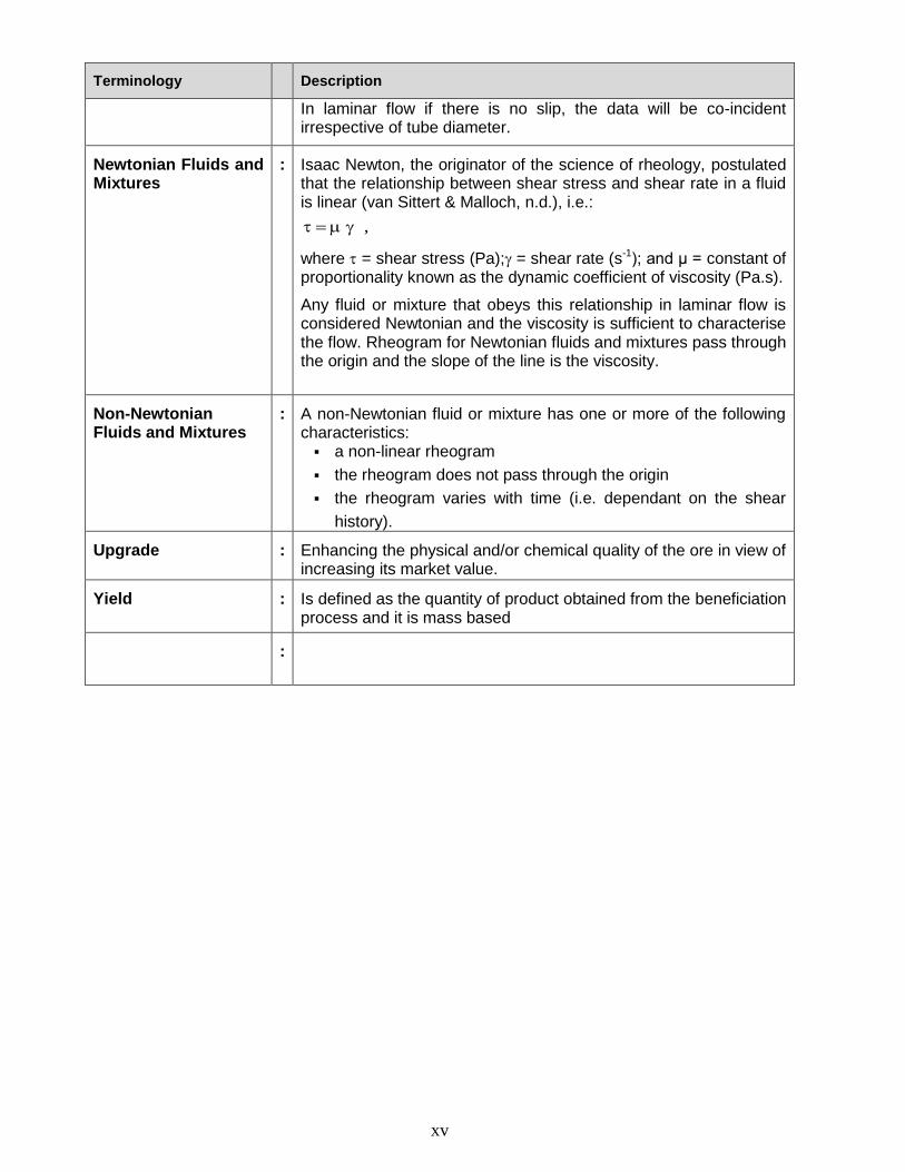
In laminar flow if there is no slip, the data will be co-incident irrespective of tube diameter.

Newtonian Fluids and Mixtures

: Isaac Newton, the originator of the science of rheology, postulated that the relationship between shear stress and shear rate in a fluid is linear (van Sittert & Malloch, n.d.), i.e.:

,

where = shear stress (Pa); = shear rate (s-1); and μ = constant of proportionality known as the dynamic coefficient of viscosity (Pa.s).

Any fluid or mixture that obeys this relationship in laminar flow is considered Newtonian and the viscosity is sufficient to characterise the flow. Rheogram for Newtonian fluids and mixtures pass through the origin and the slope of the line is the viscosity.

Non-Newtonian Fluids and Mixtures

: A non-Newtonian fluid or mixture has one or more of the following characteristics: a non-linear rheogram

the rheogram does not pass through the origin

the rheogram varies with time (i.e. dependant on the shear

history).

Upgrade : Enhancing the physical and/or chemical quality of the ore in view of increasing its market value.

Yield : Is defined as the quantity of product obtained from the beneficiation process and it is mass based

:

- 1 -

CHAPTER 1: INTRODUCTION

1 BACKGROUND

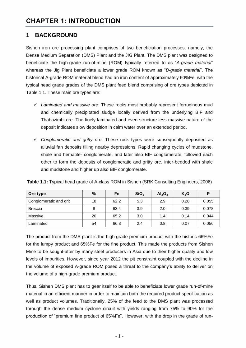
Sishen iron ore processing plant comprises of two beneficiation processes, namely, the

Dense Medium Separation (DMS) Plant and the JIG Plant. The DMS plant was designed to

beneficiate the high-grade run-of-mine (ROM) typically referred to as “A-grade material”

whereas the Jig Plant beneficiate a lower grade ROM known as “B-grade material”. The

historical A-grade ROM material blend had an iron content of approximately 60%Fe, with the

typical head grade grades of the DMS plant feed blend comprising of ore types depicted in

Table 1.1. These main ore types are:

Laminated and massive ore: These rocks most probably represent ferruginous mud

and chemically precipitated sludge locally derived from the underlying BIF and

Thabazimbi-ore. The finely laminated and even structure less massive nature of the

deposit indicates slow deposition in calm water over an extended period.

Conglomeratic and gritty ore: These rock types were subsequently deposited as

alluvial fan deposits filling nearby depressions. Rapid changing cycles of mudstone,

shale and hematite- conglomerate, and later also BIF conglomerate, followed each

other to form the deposits of conglomeratic and gritty ore, inter-bedded with shale

and mudstone and higher up also BIF conglomerate.

Table 1.1: Typical head grade of A-class ROM in Sishen (SRK Consulting Engineers, 2006)

Ore type % Fe SiO2 Al2O3 K2O P

Conglomeratic and grit 18 62.2 5.3 2.9 0.28 0.055

Breccia 8 63.4 3.9 2.0 0.39 0.078

Massive 20 65.2 3.0 1.4 0.14 0.044

Laminated 54 66.3 2.4 0.8 0.07 0.056

The product from the DMS plant is the high-grade premium product with the historic 66%Fe

for the lumpy product and 65%Fe for the fine product. This made the products from Sishen

Mine to be sought-after by many steel producers in Asia due to their higher quality and low

levels of impurities. However, since year 2012 the pit constraint coupled with the decline in

the volume of exposed A-grade ROM posed a threat to the company’s ability to deliver on

the volume of a high-grade premium product.

Thus, Sishen DMS plant has to gear itself to be able to beneficiate lower grade run-of-mine

material in an efficient manner in order to maintain both the required product specification as

well as product volumes. Traditionally, 25% of the feed to the DMS plant was processed

through the dense medium cyclone circuit with yields ranging from 75% to 90% for the

production of “premium fine product of 65%Fe”. However, with the drop in the grade of run-

- 2 -

of-mine material coupled with elevated proportion of near-density material, the performance

of dense medium cyclone plant has been impacted negatively. The current yields hardly

reach 70% with the fine product of ranging around 62.5%Fe to 63%Fe.

1.1 SISHEN DMS CYCLONE PLANT CIRCUIT

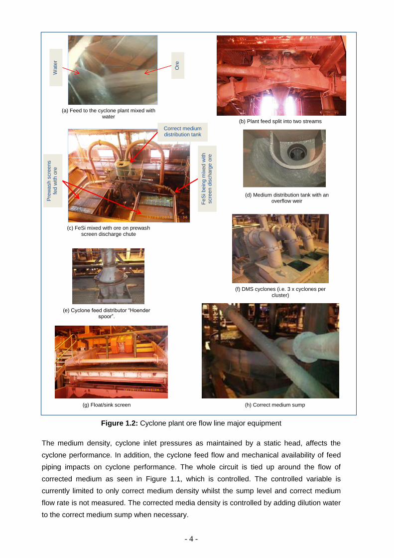
This section aims to describe the high-level process flow of the Sishen’s cyclone plant as

illustrated in Figure 1.1 with supporting major equipment depicted in Figure 1.2. As the fine

material enters the cyclone plant through the conveyors it is mixed with water as the material

is discharged into the feed sump as seen in Figure 1.2a. The ore is further split into two

separate lines as seen in Figure 1.2b to feed two prewash screening section of the module

on each side of the split. In each section, the stream is further split again into two streams

with each stream feeding a single screen module. Unfortunately, the splits causes an

uneven split of solids reporting to each screen as seen when Figure 1.2c.

The material being discharged from the screens is mixed with process FeSi from the

medium distribution tank. The FeSi in the medium distribution tank (in Figure 1.2c) has to

overflow the launder as shown in Figure 1.2d so as to ensure the correct static head is

maintained sufficient to generate the correct DMS cyclone pressures. The FeSi – Solids

mixture then flows into a distributer as seen in Figure 1.2e and is further split into three

streams with each stream flowing into a cyclone as seen in Figure 1.2f. Trial test conducted

using pressure gauges installed on some of the cyclones showed that the difference in

pressure between individual cyclones of a cluster varied widely. It is suspected that the

pressure variation is a result of the static head not being maintained and that the uneven

split of solids to each screen and subsequently each cyclone cluster. These challenges

cause unstable operation of cyclone plant. Currently the Cyclones do not have pressure

gauges installed on them.

The cyclone floats flow over the float screens to separate the solids from the FeSi and

likewise the cyclone sinks flow over the sink screen to separate the FeSi from the solids. The

separated FeSi from the float screens flows into the dilute sump while the separated FeSi

from the sink screens flows into the corrected medium tank. In order to ensure that the

correct static head is maintained for the cyclones the level of FeSi medium in the correct

medium sump has to be maintained above a certain level so that the FeSi continuously

overflows the discharge launder in the medium distribution tank. Furthermore, in order to

maintain the desired cut point it is important to accurately control the correct medium

density. Dilute medium from both the float and sink screens flows into the dilute sump, is

then pumped into the Primary and Secondary magnetic separators, and degrit cyclones to

separate the FeSi from the water and any solids associated with the stream.

- 3 -

Figure 1.1: Cyclone medium flow line

3x

Be

ne

ficia

tio

n

Cyclo

ne

s

Pre

-Wa

sh

S

cre

en

s

Sin

k

Scre

en

s

Flo

or

pu

mp

Flo

at

Scre

en

s

Pri

ma

ry M

ag

ne

tic

Se

pa

rato

r

6x

Gri

t C

yclo

ne

s

Se

co

nd

ary

Ma

gn

eti

c

Se

pa

rato

r

6x

De

wa

teri

ng

C

yclo

ne

s

Me

dia

C

on

e

De

nsif

ier

Co

ne

Dil

ute

C

on

eW

aste

Wa

ter

Ta

nk

Sp

ira

l C

lassif

ier

De

nsif

ier

Flo

at

Scre

en

s

Me

diu

mD

istr

ibu

tio

n

Ta

nk

- 4 -

Figure 1.2: Cyclone plant ore flow line major equipment

The medium density, cyclone inlet pressures as maintained by a static head, affects the

cyclone performance. In addition, the cyclone feed flow and mechanical availability of feed

piping impacts on cyclone performance. The whole circuit is tied up around the flow of

corrected medium as seen in Figure 1.1, which is controlled. The controlled variable is

currently limited to only correct medium density whilst the sump level and correct medium

flow rate is not measured. The corrected media density is controlled by adding dilution water

to the correct medium sump when necessary.

(a) Feed to the cyclone plant mixed with water

(b) Plant feed split into two streams

(d) Medium distribution tank with an overflow weir

(c) FeSi mixed with ore on prewash screen discharge chute

(f) DMS cyclones (i.e. 3 x cyclones per cluster)

(e) Cyclone feed distributor “Hoender spoor”.

(g) Float/sink screen (h) Correct medium sump

Wate

r

Ore

Pre

wash s

cre

ens

fed w

ith o

re

Correct medium distribution tank

Fe

Si bein

g m

ixed w

ith

scre

en d

ischarg

e o

re

- 5 -

1.2 PROBLEM STATEMENT

As the mining of high-grade iron ore becomes depleted, a need arises to beneficiate the low-

grade material. Figure 1.3 presents the Sishen Mine material classification as well as the

ROM feed grades to the DMS plant. It is evident that post-2010 year, the feed grade to the

DMS plant declined drastically, with an increase in the material with less 58%Fe being fed to

the plant.

A high proportion of near density waste material, which would necessitate a higher

separation density in order to effectively, and efficiently beneficiate this material normally

characterizes this low-grade ROM in order to maintain required product specification and

volumes. Thus, a much higher operating density of the ferrosilicon (FeSi) medium will be

required as well as refining the cyclone geometry and control to achieve the required

beneficiation objectives.

Figure 1.3: Material classification and DMS ROM feed grades

The current Sishen dense medium cyclone process operations is mostly reliant on operator

intervention, which include visual inspection of process, control parameter that can easily be

tracked by automated instruments. This results in an inconsistent medium balance in circuit

thereby influencing the plant efficiency. Thus, high yield losses to waste and poorer product

quality are generally noticed.

- 6 -

With the current performance of cyclone plant, an optimisation project has been undertaken

to ensure tighter control philosophy of the cyclone unit processes to ensure that it can

handle lower grade ROM material with higher near density material. This type of statement is

made on the basis that cyclone setup and operation throughout Sishen Mine is in a relatively

poor shape. This is due to number of reasons such as:

i. Incorrectly specified system setup Sishen’s cyclone plant is relatively manual

operated with limited automated control.

ii. Overfeeding

iii. Variation in medium viscosity

iv. System changes over time

v. Poor maintenance

Therefore, consistent system management, measurement and insight are required to

maximize the opportunity that the cyclones present. By modelling and simulation, the aim

should be to identify the financial benefit to be gained from better operation, automation, and

consequently, trade this off against the costs associated with operation. Moreover, it will help

to identify how much effort should be placed on this part of the operation.

1.3 RESEARCH OBJECTIVE(S):

One of the major challenges in the plant is trying to stabilise the cyclone operation and

equalising the flow of the solids through the parallel streams in the plant. In addition, the

ability of the plant to treat run-of-mine of varying grade and changing proportion of near-

density material is challenging due to the reliance on human intervention and it being manual

operated system. Thus, the main objective of the research project is to:

i. To investigate the benefit of automated control of the cyclone plant in order to stabilise

the process and manage the roping conditions.

ii. To investigate the operating conditions in order to treat the material of lower grade and

still produce product with the current quality specification.

iii. To characterise the ROM in order to understand and manage the impact of near-

density gangue material in the beneficiation of iron ore.

iv. To analyse process FeSi rheological characteristic and the ability to operate at ultra-

high densities in order to beneficiate low grade iron ore material.

v. To develop algorithms for modelling and simulating the ore and FeSi circuit for the iron

ore beneficiation in cyclone unit process.

vi. The data gathering was around the DMS on the plant and this data was used to

compare with the Simulink model.

- 7 -

This part of the cyclone optimisation project is concerned with the effectiveness of the

cyclones process and automation in order to improve operating efficiency during

beneficiation of lower grade ROM material with higher proportion of near-density material.

Furthermore, the optimisation project included the provision of a DMS model that is useful to

the personnel at Sishen without being laborious in its use and calibration.

- 8 -

CHAPTER 2: LITERATURE SURVEY

2 LITERATURE REVIEW

2.1 WHAT IS DENSE MEDIUM SEPARATION

Dense medium separation (DMS) can be defined simplistically as the practical commercial

application of the use of a fluid of some intermediate relative density to effect the separation

of a mixture of solids particles with different specific gravities. DMS as defined by (Gochin &

Smith, 1983) is a process utilised to sort particles based on their apparent density relative to

that of a carrying medium. Thus, in the DMS process, the lighter particles float on the dense

medium whilst the heavier particles sink forming a low SG and high SG fractions

respectively.

Dense medium separation has been widely used in mineral processing plants that produce

saleable products such as coal, diamonds and iron ore concentrates (Gochin & Smith,

1983). The coal washing plants mainly use magnetite medium and operated at relatively

lower densities ranging between 1250 – 1650 kg/m3, whereas the diamond and iron ore

industries utilised the ferrosilicon medium. Most of the research work and optimisation

studies in the application of DMS cyclones have focused mainly on the application of this

technology in the coal washing processes.

2.2 THEORY OF DENSE MEDIUM SEPARATION IN CYCLONE

DMS cyclones are universally standard pieces of equipment for high tonnage density

separation duties. They are essentially “plug and play” devices that are perceived to be

highly robust, particularly in terms of performance under a wide range of operating

conditions. This perception is further entrenched by the use of a single performance

indicator, the cut point density, which trivializes the complexity of the device.

The principle of operation of dense medium cyclone, as described by (King, 2001) and

(http://www.portaclone.co.za/pr_cyclo.htm) is based on the fluid pressure energy that

creates a rotational fluid motion as result of tangential feed of the dense medium in the

cyclone. There are two main factors influencing the separation efficiency in a cyclone. These

are the force ratios in the cyclone and the cyclone geometry. Figure 2.1 graphically presents

the particle motion taking place inside the cyclone as well as the forces acting on the particle

suspended in the dense medium. There are three major forces (i.e. centrifugal, drag, and

gravitational force) acting on the solid particles as they travel radially and helically inside the

cyclone body, forcing the heavier particles toward the wall of the body and the lighter

particles toward the centre.

The centrifugal field generated by high circulating velocities in the cyclone to creates an air

core on the axis that usually extends from the spigot opening at the bottom of the conical

http://www.portaclone.co.za/pr_cyclo.htm

- 9 -

section through the vortex finder to the overflow at the top. The air core creates a force high

enough to drag lighter mixture of particles and medium towards the vortex finder. Thus, the

fluid leaving via the vortex finder carries the lighter particles with it while the centrifugal force

causes heavy and large particles to migrate towards the cyclone wall and there descend to

leave via the spigot.

In addition, it has been described that there is an envelope of zero velocity (i.e. Fc = Fdrag)

inside the cyclone where the near-density material normally is trapped. This trapped material

has equal probability to be misplaced to either the underflow or the overflow. Thus, adjusting

the vortex finder and spigot diameter would allow shifting the cut-size to a range where the

impact of near-density material is minimised.

Figure 2.1: Typical cyclone equipment showing (a) Particle trajectory, and (b) Forces acting

on a particle in a cyclone. (King, 2001); (Anon., n.d.),

These forces influencing the separation efficiency in a cyclone are being imparted on a

particle inside a normal cyclone and summarised as follows:

i. Centripetal Force: Due to the velocity of the material as it enters the cyclone, a

centripetal force is exerted on the particles as they change from a linear motion to a

circular motion. This force, when dominant, will cause the particles to report to the

peripheral of the cyclone and hence to the cyclone spigot. The force is a function of

the particle mass and subsequently the density and the tangential velocity in the

cyclone.

2VF lCentrifuga , with V being the tangential velocity in the cyclone.

(a) (b)

- 10 -

ii. Drag Forces: Drag forces are imparted to the particles, primarily by the volumetric

flow rate to the cyclone vortex finder. The drag force is dependent on the fluid

velocity and particle velocity in the cyclone in the following relationship:

pfDrag UUF , where Uf is the velocity of the fluid and Up is the velocity of the

particle.

iii. Buoyancy Force: Buoyancy force is a function of the density and stability of the

medium. The buoyancy force can be either in the direction of the cyclone wall or the

air core depending on the density and size of the particle. The relationship between

buoyancy force and tangential velocity in the cyclone is the same as for centripetal

forces.

2VFBuoyancy

iv. Gravity Force: This force is ignored due to dynamic nature of separation in the

cyclone.

To understand the effect that the above mentioned forces will have on the separation

efficiency in the DMS cyclone, JKMRC did some test work showing a density profile in a

cyclone (at a feed density of 1.40g/cm3) constructed by means of gamma radiation

tomography. Although this experiment was conducted using magnetite, the principle will be

similar for a cyclone operating with ferrosilicon. Figure 2.2 is a graphical representation of

the tomography results by (Wang, 2009) and (Narasimha, et al., 2006).

Figure 2.2: Tomogram at feed density of 1.40 g/cm3

Looking at the density profile between the air core and the cyclone wall at the top of the

cyclone cone, the differential is no more than 0.02 ranging from 1.30 t/m3 to 1.50 t/m3. It is

only in the spigot area that the density profile starts to change, increasing to a density of

- 11 -

1.70 t/m3 and above. Applying this principle to a cyclone operating with ferrosilicon at a feed

density of 3.60 t/m3, similar density distributions can be assumed as presented in Figure 2.3.

Due to its size, the cyclone spigot can only handle a certain amount of material reporting to

the cyclone underflow before inefficiencies will start to occur. In the past it was believed that

only the high-density material (+3.60 t/m3) reported to the spigot area while the lower density

material (-3.60 t/m3) reports to the cyclone overflow through the vortex finder while still in the

cyclone barrel.

From Figure 2.3 it is evident that the +3.40 t/m3 – 3.80 t/m3 material will report to the spigot

area where it will encounter medium densities of 3.80 t/m3 and higher. These spigot

densities will force the material with densities below 3.80 t/m3 back to the vortex finder to the

cyclone overflow with the rest of the low-density material. To ensure efficient separation in

the cyclone spigot of the high-density material (+3.80t/m3) to the cyclone underflow and the

low-density material (<3.80t/m3) to the cyclone overflow, the material loading in the spigot

areas must not exceed 80%.

Figure 2.3: Tomogram at assumed density profile at feed density of 3.60 t/m3

2.2.1 Factors Influencing Dense Medium Beneficiation

The summary of major factors that affect the dense medium cyclone performance as well as

its performance indicators are explained by He and Laskowski (1995a) as cited by (Sripriya,

et al., 2001). The factors that include three groups of variables are illustrated in Figure 2.4

and include the following: (i) medium composition, (ii) feed characteristics, and (iii) cyclone

operating conditions.

i. Medium composition: medium composition affects beneficiation process

performance by changing its stability and rheology. The impact of medium stability in

cyclone performance can be characterised by the density differential between the

cyclone overflow and underflow streams.

2.65g/cm3

2.7g/cm3

2.8g/cm3

3.1g/cm3

3.60t/m3

3.65t/m3

3.70t/m3

3.90t/m3

Assum

ed d

ensity p

rofile

- 12 -

ii. Feed characteristics: is mainly determined by the particle size, particle shape,

proportion of near-density material as well as the feed rate.

iii. Operating conditions: this can be summarised as the (a) inlet pressure; (b) medium

density; (c) medium flow rate; (d) medium split and (e) medium-to-ore ratio.

Figure 2.4: Performance indicators and factors affecting dense medium cyclone

performance

Med

ium

Co

mp

osit

ion

•Siz

e d

istr

ibu

tio

n

•So

lids c

on

ten

t

•Cla

y c

on

tam

ina

tio

n

•Pa

rtic

le s

ha

pe

an

d d

en

sity

DM

S P

ERFO

RM

AN

CE

•C

ut-

po

int

shif

t

•Ep

valu

e

Med

ium

Rh

eo

log

y

•Yie

ld s

tre

ss

•Vis

co

sity

Old

(Lo

w S

ph

eri

city

)Im

pro

ved

sp

he

rici

ty

Med

ium

Sta

bilit

y

•De

nsity d

iffe

rentia

l

Op

era

tin

g C

on

dit

ion

s

•In

let p

ressu

re

•Me

diu

m f

low

ra

te

•Me

diu

m s

plit

•Me

diu

m-t

o-o

re r

atio

Flo

w m

eter

Pre

ssu

re

Tran

smit

ter

Sum

p L

eve

l In

dic

ato

r

Nucleonic

Densitometer

Feed

Ch

ara

cte

risti

cs

•Siz

e d

istr

ibu

tio

n

•Pa

rtic

le s

ha

pe

•Ne

ar

de

nsity m

ate

ria

l

•RO

M c

om

po

sitio

n &

Fe

gra

de

Eq

uip

men

t G

eo

metr

y

•C

yclo

ne

dia

me

ter

•S

pig

ot siz

e &

we

ar

rate

•C

om

po

ne

nt m

isa

lign

me

nt/

inw

ard

ste

pp

ing

•D

rum

skirtin

g h

eig

ht/

len

gth

•D

rum

th

in r

ub

be

r h

eig

ht/

len

gth

•D

rum

lifte

r co

nd

itio

ns

- 13 -

2.2.2 Importance of Dense Medium Rheological Characteristics

Rheology has been described in literature as the science dealing with flow and deformation

of matter. It can be defined as the viscous characteristics of a fluid or homogenous solid-

liquid mixture. The term homogenous indicate that the solids particles are uniformly

distributed across the medium carrier whilst the viscous indicate that laminar flow condition

is considered as opposed to turbulent flow regime.

The heavy liquid medium used for the dense medium is classified as a non-Newtonian slurry

mixture and its flow behaviour can be models by various rheological mathematical models.

Rheological models are applied on the rheogram in order to transform them to information

on the fluid rheological behaviour (Björn, et al., 2012). Non-Newtonian fluid or mixture can be

characterised by one of the following characteristics such as (i) a non-linear rheogram; (ii)

the rheogram does not pass through the origin; and (iii) the rheogram varies with time, which

is, depended on the shear history.

According to van Sittert & Malloch (n.d.) and Bjorn et al (2012) the most suitable

mathematical models for most of the non-Newtonian fluid or mixture and mineral slurry

application is the generalised yield pseudo-plastic or Herschel Bulkley model and Bingham

model. Rheological models as found in literature are summarized in Table 2.1 while typical

rheogram for different models are graphically illustrated in

Figure 2.5.

Table 2.1: Rheological models

Model Yield Stress Fluid Behaviour

Index

Constitute Equation

Newtonian y = 0 n = 1 τ = μγ

Bingham plastic y > 0 n = 1 τ = τy + Kγ

Pseudo-plastic y = 0 n < 1 τ = Kγn

Yield pseudo-plastic y = 0 n < 1 τ = τy + Kγn

Dilatant y = 0 n > 1 τ = Kγn

Yield Dilatant y > 0 n > 1 τ = τy + Kγn

In addition, the rheological properties of heavy medium can be represented in plotted

pseudo shear diagram using a data generated from the vertical loop pipe test. This is a plot

of wall shear stress versus pseudo shear rate. The pseudo-shear rate is defined as (van

Sittert & Malloch, n.d.):

,D

V8 m …Equation 2.1

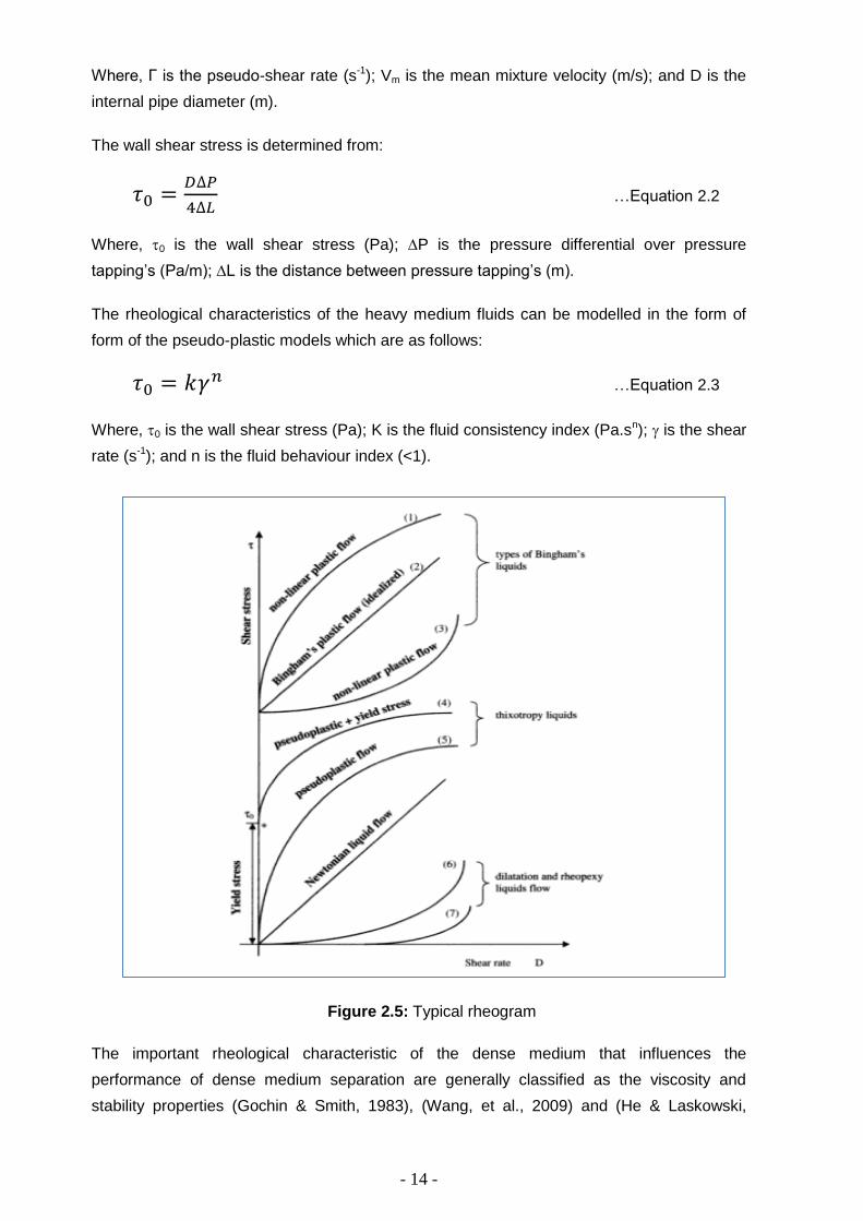
- 14 -

Where, Γ is the pseudo-shear rate (s-1); Vm is the mean mixture velocity (m/s); and D is the

internal pipe diameter (m).

The wall shear stress is determined from:

𝜏0 =𝐷∆𝑃

4∆𝐿 …Equation 2.2

Where, 0 is the wall shear stress (Pa); P is the pressure differential over pressure

tapping’s (Pa/m); L is the distance between pressure tapping’s (m).

The rheological characteristics of the heavy medium fluids can be modelled in the form of

form of the pseudo-plastic models which are as follows:

𝜏0 = 𝑘𝛾𝑛 …Equation 2.3

Where, 0 is the wall shear stress (Pa); K is the fluid consistency index (Pa.sn); is the shear

rate (s-1); and n is the fluid behaviour index (<1).

Figure 2.5: Typical rheogram

The important rheological characteristic of the dense medium that influences the

performance of dense medium separation are generally classified as the viscosity and

stability properties (Gochin & Smith, 1983), (Wang, et al., 2009) and (He & Laskowski,

- 15 -

1994). The viscosity is described as a measure of the resistance to flow of a liquid and

influences the movement of ore particles through the dense medium. On the other hand,

stability controls the medium segregation in the cyclone that leads to a phenomenon known

as cyclone differential. Cyclone differential is defined as the density differential of the

medium reporting to the floats stream and that to the sinks stream of the unit process.

In a separating medium (typical of DMS operations) it is determined largely by the

concentration, shape and size distribution of the solids making up the medium. Viscosity is

measured for particular shear rates in units of cP (centipoise), the SI equivalent being Ns/m2.

A high viscosity results from high solids concentration, fine particle size distribution, irregular

shapes, and presence of low density contaminant solids. A low viscosity results from the

converse of the above.

Medium viscosity is an important property, and given the difficulty of measurement, its

influence on separation is not always completely understood. In general too high viscosity

values are not desirable because of reduced separation velocities, increasing probability of

particle misplacement and reduced partition efficiencies.

The literature described that the rheological properties of the dense medium are one of the

key factors that influence/affects the separation efficiency cyclone systems. The influence of

medium rheological properties on cyclonic dense medium system can be summarised as

follows:

a) Coarser ferrosilicon medium at lower medium densities results in excessive media

segregation that leads to a higher density differential due to unstable medium. Higher

density differential are responsible for high cut-point shifts and leads to longer

retention time of near density material in the cyclone.

b) According to (Wang, et al., 2009), the density differential was found to decrease as

the non-magnetic content of the medium increases.

c) In order to achieve satisfactory separation in cyclonic systems, (Napier-Munn, et al.,

1994) and (He & Laskowski, 1994) recommended that density differential be

maintained within 0.2 and 0.5 SG.

d) Increase in medium density, coupled with the fine particle size distribution of media

and presence of low density slimes (contaminating non-magnetics) would result in an

increase in medium viscosity.

e) A summary of factors contributing and influencing media rheology are described by

(Myburgh, 2006) which is graphically depicted in Figure 2.6. These included; (i) slime

(non-mag) content, (ii) media shape and (iii) ultrafine content (percentage of -45µm).

- 16 -

The proportion of the ultra-fine is required to maintain the optimal operating

differential for cyclonic system in Sishen averaged around 62%.

f) High viscosity media is undesirable because they reduce the velocity of mineral

particles being separated thereby increasing the probability of particle misplacement

and reducing the efficiency of separation.

Figure 2.6: Schematic explanation of variables on medium rheology

2.2.3 Cyclone Performance Measure

The performance of the cyclone unit process is generally determined by the Ecart Probable

Moyen (Ep-value). The Ep value describes the separating efficiency of the unit process

regardless of the quality of feed material (Wills & Napier-Munn, 2006); (Gochin & Smith,

1983). The Ep is determined from the slope of the tromp curve which represents the

probability of the percentage of the feed material that will report to either the sinks or floats

depending on their relative density distribution.

- 17 -

A typical tromp curve as well as operating Ep values of separating unit processes are

graphically presented in Figure 2.7. In addition, Figure 2.7(b) shows the effect of particle size

on the efficiency of dense media separating unit process. The lower the Ep value, the better

the efficiency of the equipment. Typical acceptable Ep values for the cyclone module range

between 0.05 - 0.10 for the iron ore beneficiation. The probability curve (Tromp curve) in

conjunction with the Ecart Probable Moyen was used to demonstrate the impact of

processing efficiency of material with different densimetric profiles.

The partition curve is determined using the Whitten’s equation for beneficiation process

without short-circuiting (Wills & Napier-Munn, 2006):

PN =1

[1+exp(k(ρ50−ρi)

Ep)]

….Equation 2.4

With, k = 1.098 (constant determined experimentally); 50 = cut-point density; i = density

fraction and Ep = separation efficiency.

Figure 2.7: Graphical representation of (a) Tromp curve, and (b) Ep vs. Particle size. (Wills

& Napier-Munn, 2006)

Some of the critical process and operating parameters that are critical for the efficient

operation of dense medium cyclone circuits as described by (Bekker, 2012) and (Atkinson,

et al., 2012) includes:

(i) Washability of material which is related to yield,

(ii) Feed particle size distribution,

(iii) Head (D) and head loss, with the normal head for mineral industry is 7 – 20 x D.

According to (Atkinson, et al., 2012), lower head, (e.g. <7D), is not desirable for

beneficiation of fine material. In addition, it has been alluded that higher operating

head results in high cut-point shift and thus are not recommended in operation

where high cut-point densities are not desirable.

(a) (b)

- 18 -

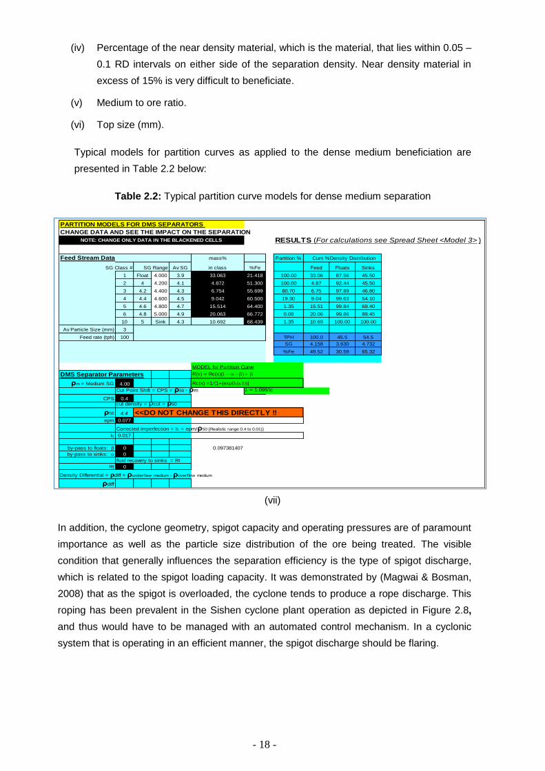
(iv) Percentage of the near density material, which is the material, that lies within 0.05 –

0.1 RD intervals on either side of the separation density. Near density material in

excess of 15% is very difficult to beneficiate.

(v) Medium to ore ratio.

(vi) Top size (mm).

Typical models for partition curves as applied to the dense medium beneficiation are

presented in Table 2.2 below:

Table 2.2: Typical partition curve models for dense medium separation

(vii)

In addition, the cyclone geometry, spigot capacity and operating pressures are of paramount

importance as well as the particle size distribution of the ore being treated. The visible

condition that generally influences the separation efficiency is the type of spigot discharge,

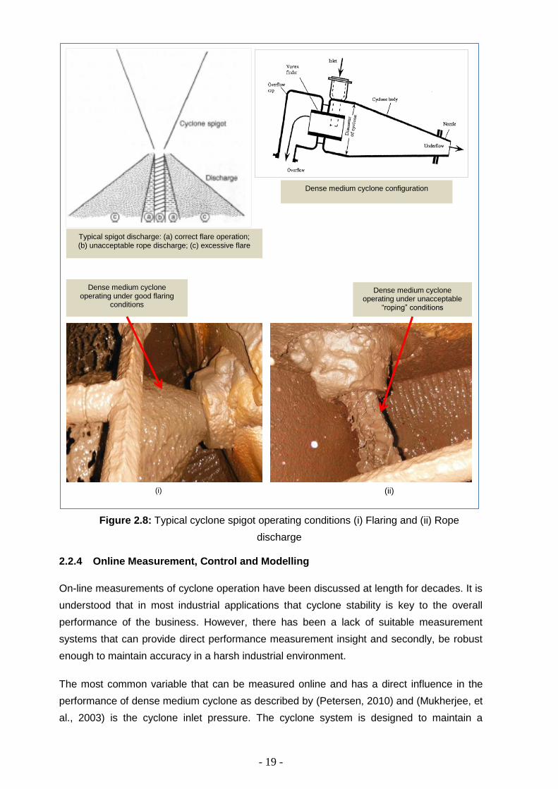
which is related to the spigot loading capacity. It was demonstrated by (Magwai & Bosman,

2008) that as the spigot is overloaded, the cyclone tends to produce a rope discharge. This

roping has been prevalent in the Sishen cyclone plant operation as depicted in Figure 2.8,

and thus would have to be managed with an automated control mechanism. In a cyclonic

system that is operating in an efficient manner, the spigot discharge should be flaring.

PARTITION MODELS FOR DMS SEPARATORS

CHANGE DATA AND SEE THE IMPACT ON THE SEPARATION

RESULTS (For calculations see Spread Sheet <Model 3> )

Feed Stream Data mass% Partition % Cum %Density Distribution

SG Class # SG Range Av SG in class %Fe Feed Floats Sinks

1 Float 4.000 3.9 33.063 21.418 100.00 33.06 87.56 45.50

2 4 4.200 4.1 4.872 51.300 100.00 4.87 92.44 45.50

3 4.2 4.400 4.3 6.754 55.699 80.70 6.75 97.89 46.80

4 4.4 4.600 4.5 9.042 60.500 19.30 9.04 99.63 54.10

5 4.6 4.800 4.7 15.514 64.400 1.35 15.51 99.84 69.40

6 4.8 5.000 4.9 20.063 66.772 0.08 20.06 99.86 89.45

10 5 Sink 4.3 10.692 68.439 1.35 10.69 100.00 100.00

Av Particle Size (mm) 3

Feed rate (tph) 100 TPH 100.0 45.5 54.5

SG 4.158 3.630 4.732

%Fe 49.52 30.59 65.32

MODEL for Partition Curve

DMS Separator Parameters R(x) = Rc(x)(1 b) + b

ρm = Medium SG 4.00 Rc(x) =1/(1+(exp(λ(x-1))]

Cut Point Shift = CPS = ρ50 - ρm λ = 1.099/Ic

CPS 0.4cut density = ρcut = ρ50

ρ50 4.4 <<DO NOT CHANGE THIS DIRECTLY !!epm 0.077

Corrected imperfection = Ic = epm/ρ50 {Realistic range 0.4 to 0.01)}

Ic 0.017

by-pass to floats: b 0 0.097381407

by-pass to sinks: 0

fluid recovery to sinks = Rf

Rf 0

Density Differential = ρdiff = ρunderflow medium - ρoverflow medium

ρdiff

NOTE: CHANGE ONLY DATA IN THE BLACKENED CELLS

- 19 -

Figure 2.8: Typical cyclone spigot operating conditions (i) Flaring and (ii) Rope

discharge

2.2.4 Online Measurement, Control and Modelling

On-line measurements of cyclone operation have been discussed at length for decades. It is

understood that in most industrial applications that cyclone stability is key to the overall

performance of the business. However, there has been a lack of suitable measurement

systems that can provide direct performance measurement insight and secondly, be robust

enough to maintain accuracy in a harsh industrial environment.

The most common variable that can be measured online and has a direct influence in the

performance of dense medium cyclone as described by (Petersen, 2010) and (Mukherjee, et

al., 2003) is the cyclone inlet pressure. The cyclone system is designed to maintain a

(i) (ii)

Typical spigot discharge: (a) correct flare operation; (b) unacceptable rope discharge; (c) excessive flare

Dense medium cyclone operating under good flaring

conditions

Dense medium cyclone operating under unacceptable

“roping” conditions

Dense medium cyclone configuration

- 20 -

specific inlet pressure, which would indicate that the flow rate is then within specification.

Thus, inlet pressure measurement is most commonly used for cyclone system stability. Inlet

pressure is currently not measured at Sishen due to the harshness of the environment.

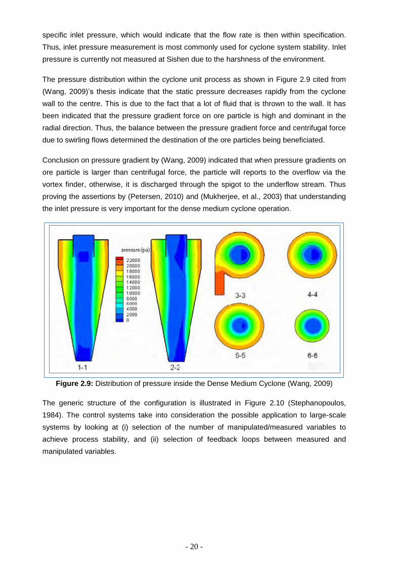
The pressure distribution within the cyclone unit process as shown in Figure 2.9 cited from

(Wang, 2009)’s thesis indicate that the static pressure decreases rapidly from the cyclone

wall to the centre. This is due to the fact that a lot of fluid that is thrown to the wall. It has

been indicated that the pressure gradient force on ore particle is high and dominant in the

radial direction. Thus, the balance between the pressure gradient force and centrifugal force

due to swirling flows determined the destination of the ore particles being beneficiated.

Conclusion on pressure gradient by (Wang, 2009) indicated that when pressure gradients on

ore particle is larger than centrifugal force, the particle will reports to the overflow via the

vortex finder, otherwise, it is discharged through the spigot to the underflow stream. Thus

proving the assertions by (Petersen, 2010) and (Mukherjee, et al., 2003) that understanding

the inlet pressure is very important for the dense medium cyclone operation.

Figure 2.9: Distribution of pressure inside the Dense Medium Cyclone (Wang, 2009)

The generic structure of the configuration is illustrated in Figure 2.10 (Stephanopoulos,

1984). The control systems take into consideration the possible application to large-scale

systems by looking at (i) selection of the number of manipulated/measured variables to

achieve process stability, and (ii) selection of feedback loops between measured and

manipulated variables.

- 21 -

Figure 2.10: General structure of the control configuration (Stephanopoulos, 1984)

Met Coal and Venetia mine’s unit processes have pressure transmitter and gauges installed,

which are used for control purpose. Venetia Mine is maintaining a balanced static head

across operating modules thereby ensuring stable inlet pressures in all operating cyclones.

This showed a great improvement in processing and beneficiation efficiency

Therefore, Sishen Mine can learn from their system of ensuring that all operating cyclones

maintain similar feed pressure. Figure 2.11 shows the installation of pressure transmitters at

Capcoal and Venetia Mines whilst Figure 2.12 present Venetia’s innovative system to ensure

medium balance in the circuit thereby achieving constant cyclone pressure across operating

modules for their gravity fed system.

(a) (b)

Figure 2.11: (a) Capcoal and (b) Venetia’s cyclone inlet pressure instruments

Beneficiation Process Manipulated

Variables

EXTERNAL DISTURBANCES

Unmeasured (d’) Measured (d)

Measured

Outputs

Unmeasured outputs

Estimator: computes an estimate of

the values of the unmeasured

controlled variables

Controller

Set points

Pressure

transmitter

Pressure gauge

Cyclone

feed pipe

Pressure transmitters

- 22 -

Figure 2.12: Venetia’s medium head balance across module and its impact of cyclone inlet pressure

Flow rate measurement is possibly the other most important piece of information that could

be obtained from a cyclone system. Magnetic flow rate meters are common equipment in the

minerals industry, but can only be used if the material being processed is non-magnetic.

Advances that are more recent have shown the development of the ring impulse flow-rate

measurement scheme, which attaches approximately eight (8) rings around the inlet of the

cyclone and disturbances within the fluid are picked up by all eight (8) rings, which are then

correlated to determine the movement of the disturbances, which is then turned into flow-

rate estimation. Sishen is considering the installation of SONARtrac flow meters, which are

non-slurry contact unit and thus will not be subjected to high abrasive environment in the

DMS circuit.

Modelling of the performance of the dense medium separation can be performed using a

Simulink program based on the existing models from literature. Such models includes

empirical models developed by many researchers on the predictions of performance of the

dense medium cyclone are well summarised by (Wang, 2009). The well-known model is the

Wood’s empirical model with heavy reliance on many fitting factors. The use of the model is

to assess the likelihood of the outlet overloading, particle retention as well as surging. The

basic structure of the Wood’s Model is as follows:

i. The main state equation is that of flow rate (Qf) which includes both medium and ore:

QF = K ∙ D1.48 ∙ R0.15 ∙ H0.45 …Equation 2.5

Initial set-up leading to imbalance medium head for different led to high variation in module operating pressures.

Optimised system to balance medium head across modules significant minimization of pressure variation.

- 23 -

ii. The flow split of medium only:

𝑄𝑢𝑧

𝑄𝑓𝑧= 0.79𝐻𝑒𝑎𝑑−0.37 (

𝐷𝑢

𝐷𝑜)

4.2

…Equation 2.6

The above equation then acknowledges that the presence of ore modifies the

medium flow split, via Qum:

𝑄𝑢𝑚 = 0.97𝑄𝑢𝑠 +𝑄𝑢𝑧

2

𝑄𝑢𝑠+𝑄𝑢𝑧 …Equation 2.7

Percentage of medium split to overflow can also be determined by the following

equation:

𝑂𝑣𝑒𝑟 % = 𝐾 ∙ (𝐷0

𝐷𝑢)

2

∙ 𝜌𝑓𝑚−1 ∙ 𝑃 ∙ (𝑀: 𝑂)0.25 …Equation 2.8

iii. Now the density of the spigot medium is calculated, um:

𝜌𝑢𝑚 = 0.459𝜌𝑓𝑚 (𝑄𝑢𝑚

𝑄𝑓𝑚)

(0.194(𝜌𝑓𝑚−2.04))

𝑃𝑅𝑅0.17𝐻𝑒𝑎𝑑0.082𝐷𝑐

0.010 …Equation 2.9

iv. Overflow density, om:

𝜌𝑜𝑚 = 𝜌𝑓𝑚 [(1−

𝑄𝑢𝑚𝑄𝑓𝑚

∙𝜌𝑢𝑚∙𝜌𝑓𝑚

)

(1−𝑄𝑢𝑚𝑄𝑓𝑚

)

] …Equation 2.10

Where Qfm; Qum; is the flow rate feed and underflow medium respectively;

Qfz; Quz is flow rate of feed; underflow with non-medium solids respectively;

Qus is the solids flow rate of underflow;

“Head” is the inlet pressure head in meters of medium;

PRR is the intercept (63.2%) of a Rosin-Rammler medium size distribution

Du is the inside diameter of the spigot;

Do is the inside diameter of the vortex finder;

K is the constant;

fm; um; om is the feed, underflow and overflow density of medium

respectively;

The control of the correct medium sump and/or tank is one of the critical part in the dense

medium separation. In most cases, these sumps/tanks tank design are truncated conical

tank. Thus, the equations 2.11 to 2.13 are applicable for determining the capacity of the

correct medium tank for a cyclone module:

Slant height: s = √(𝑅 − 𝑟)2 + ℎ2 … Equation 2.11

Total surface area: A = π[(𝑅 + 𝑟)𝑠 + 𝑅2 + 𝑟2] … Equation 2.12

- 24 -

Volume: V =1

3𝜋ℎ(𝑅𝑟 + 𝑅2 + 𝑟2) … Equation 2.13

To simplify the modelling of the tank height in order to determine when manual “fresh FeSi

addition” must happen, it was assumed that the effective area of the medium tank does not

change with change in medium height in the tank. Thus, the modelling of rate of change of

medium level in the tank can be simulated utilising the conservation of mass taking into

account the rate of medium flow in and out of the tank as follows:

𝐴𝑡𝑑ℎ𝑡

𝑑𝑟= 𝑄𝑡,𝑚𝑒𝑑 + 𝑄𝑡,𝑑𝑖𝑠 − 𝑄𝑡 … Equation 2.14

- 25 -

CHAPTER 3: METHODOLOGY

3 EXPERIMENTAL APPROACH

The experimental procedure was sub-divided into three parts: (i) ore characterisation, (ii)

characterisation of process FeSi and (iii) automation of one cyclone plant module and

processing of ROM of varying grades and evaluating performance and efficiency.

3.1 ORE CHARACTERIZATION

Ore characterisation entailed testing of various ore types and ROM blends of varying quality

for densimetric analysis; mineralogical and chemical analysis. This characterisation work

was conducted at Sishen Mine, with some of the samples dispatched to external laboratories

such as Anglo Research, Mintek and UIS Analytical Services. The equipment that was used

for the densimetric analysis of the ore material is discussed briefly below:

i. Semi-automated sink-float column and static bath sink-float set-up located at Sishen

Met Lab and Anglo Research Laboratories. Drawing and pictures of the automated

sink-float column as not shown as they might be violating the intellectual property of

the designer.

ii. XRF & QEMSCAN: Anglo Research. Figure 3.1 illustrates pictures of the XRF and

QEMSCAN machines used for chemical in Sishen and Anglo Research Labs.

Figure 3.1: Typical XRF and QEMSCAN Set-up in Sishen and Anglo Research labs

3.2 PROCESS FESI CHARACTERIZATION

Process FeSi sample was characterised at Paterson & Cooke Consulting Engineers (P&C)

Laboratories in Cape Town for rheological properties for application at ultra-high density set-

up. The schematic diagram of vertical tube viscometer set-up at P&C Labs illustrated in

Figure 3.2. A Warman 2 × 1½ AH pumps slurry through a vertical pipe of 19.6 mm internal

diameter to form a re-circulating pipe loop. Differential pressure transducers measure the

- 26 -

pressure difference across sections on the up and down legs of the pipes. A cooling jacket

cools down the slurry temperature during testing. The loop is fitted with a coriolis mass flow

meter for measuring flow rate, slurry density and temperature. The pump is fitted with a

mechanical seal to prevent dilution of the slurry.

The FeSi characterisation was subdivided as follows:

i. Medium stability test: The medium stability test measure the rate at which the

heavy medium liquid settles in a bench top scale settling test procedure. The

procedure is similar to the test conducted for determining the slurry settling rate as

well as the design of slurry thickening system. The aim of the static bench top settling

tests provides an indication of the rate at which surface water separates from the

solids for a given slurry mixture. The rate at which the slurry/water interface settles is

recorded as a function of time. During static settling test a 500 ml of sample, made

up to the correct density, is shaken vigorously and allowed to settle in a 500 mℓ

measuring cylinder. A plot of the interface height of the supernatant water above the

suspended solids over time is recorded.

ii. Rheology test work: Sishen Mine supplied P&C with a sample of the “ideal” FeSi,

which was tested to characterise the rheology of the FeSi. The viscosity is problematic

to measure as the solids settles out in conventional viscometers. It was proposed to

measure the viscosity in a re-circulating vertical tube viscometer using small bore

pipelines. The FeSi was tested over a range of concentrations to determine the change

in viscosity as a function of slurry concentration. Once the flow behaviour of the FeSi

was benchmarked, a number ways of maintaining lower viscosities at high FeSi

densities were investigated which are discussed below.

iii. Changing FeSi material properties to improve rheological flow behaviour:

o Particle Size Distribution: Changing the particle size distribution of the FeSi can result

in improved “lower” viscosity values and better stability at high FeSi densities.

Changes to the FeSi particle size was conducted by removing of the finer fraction for

both the dry coarse FeSi as well as the process FeSi. The influence of finer fraction

removal is then mathematically modelled using the Rosin-Rammler equation so as to

quantify the difference observed as follows (Doll, 2014):

𝑌 = 𝑛𝑋 − 𝑛 ln(𝐷𝑛) … Equation 3.1

Where, 𝑌 = ln(− ln 𝑅) and 𝑋 = ln(𝐷); Dn and n are fitting parameters.

The general Rosin-Rammler equation is as follows:

𝑅 = 𝑒−(𝐷

𝐷𝑛⁄ )

𝑛

… Equation 3.2

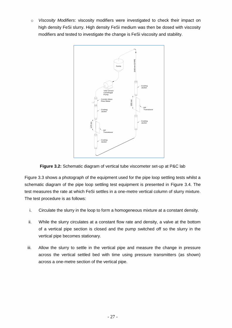
- 27 -

o Viscosity Modifiers: viscosity modifiers were investigated to check their impact on

high density FeSi slurry. High density FeSi medium was then be dosed with viscosity

modifiers and tested to investigate the change is FeSi viscosity and stability.

Figure 3.2: Schematic diagram of vertical tube viscometer set-up at P&C lab

Figure 3.3 shows a photograph of the equipment used for the pipe loop settling tests whilst a

schematic diagram of the pipe loop settling test equipment is presented in Figure 3.4. The

test measures the rate at which FeSi settles in a one-metre vertical column of slurry mixture.

The test procedure is as follows:

i. Circulate the slurry in the loop to form a homogeneous mixture at a constant density.

ii. While the slurry circulates at a constant flow rate and density, a valve at the bottom

of a vertical pipe section is closed and the pump switched off so the slurry in the

vertical pipe becomes stationary.

iii. Allow the slurry to settle in the vertical pipe and measure the change in pressure

across the vertical settled bed with time using pressure transmitters (as shown)

across a one-metre section of the vertical pipe.

Coriolis Mass

Flow Meter

Sump

VSD Driven

Centrifugal

Pump

Cooling

Jacket

DP

Transducer

Cooling

Jacket

Cooling

Jacket

1470

mm

2055

mm

DP

Transducer

Cooling

Jacket

19.6

0 m

m ID

PIP

E

- 28 -

Figure 3.3: Photograph of pipe loop settling test equipment

Figure 3.4: Schematic diagram of pipe loop settling test equipment

3.2.1 Coarse FeSi Less Fines

The “coarse FeSi less fines” was made up by blending a 1-tonne bag labelled “Coarse FeSi”

and removing a percentage of the 40 µm fraction by sieving and using Cape Town potable

tap water to make up the slurry.

3.2.2 Process FeSi

P&C tested a sample of process FeSi by blending the remains of the three drums of damp

process FeSi with the sample as received to generate one process FeSi sample. Process

FeSi was made up using the process water supplied by Kumba Iron Ore Sishen Mine.

- 29 -

3.2.3 Process FeSi Less Fines

The process FeSi, with a percentage of the 40 µm fraction removed by screening, was made

up using the process water supplied.

3.2.4 Viscosity Modifier

The viscosity modifier used for this test work was the DP 725 from Lignotech. It is a purified

grade calcium lignosulphonate product with low insoluble content and near neutral pH.

Appendix B.1 shows the specifications for DP 725. The modifier was added at a rate of

100 ml/dry tonne FeSi.

3.3 PILOT TESTING OF AUTOMATED CYCLONE MODULE

The aim of the automated pilot testing was to evaluate the benefit of managing metallurgical

variables through installation of instruments that would maintain tight control over the

process variables and thus improve performance. Such process variables that had to be

controlled include among others the following:

o Medium-to-Ore ratio: it has been demonstrated that the optimum M:O in spite of the

amount of near density material ensures good separation efficiencies. Therefore, the

“automation of the M:O ratio” is a critical aspect that must be explored further.

o Medium viscosity: it is a known fact that a viscous media is one of the critical factors

in dense medium separation process. Thus, viscosity measurement and their control

are beneficial to the dense media separation circuit.

o Ep (E-cart probable): understanding the plant controls that would allow operation to

control the Ep is also a key factor that the BU’s has to consider.

o Operating pressure: it is important to understand what the optimum operating

pressure for a particular commodity is. Therefore, a clear understanding of what test

work methodology will prove this is also critical and how to automatically manage its

influence on plant performance.

In addition, the pilot testing will unpack the factors influencing the M:O ratio and how to

mitigate the negative impact on beneficiation process. Intensive effect of M:O ratio on dense

medium separation was studied by (Chu, et al., 2009) and the following was established:

At low M:O ratio, there are heavy particles that reports to the overflow stream,

Decrease in M:O ratio increase the intensity of the inter-particle interaction thereby

affecting the partition performance of the dense medium cyclone.

As the M:O ratio decreases, the total inter-particle force, particle-wall contact force,

fluid drag force and pressure gradient force increases. This will result in an increase

- 30 -

random movement of particles thereby leading to deterioration of the partition

performance.

Lower M:O will also result in surging phenomenon, thereby misplacing the lighter

material onto the cyclone underflow streams. Thus, for the iron ore beneficiation, this

will be detrimental to the product quality.

The cyclone inlet pressure and the factors influencing the cyclone inlet pressure as well as

how they impact on the performance of the plant will be reviewed. (Petersen, 2010) alluded

to the fact that the cyclone inlet pressure has been historically used as a diagnostic measure

that work is done within the cyclone and not the actual energy doing the work. Sufficient inlet

pressure and inlet velocity lead to tangential rotation of the fluid mixture within the cyclone as

it move towards the vortex finder or the spigot (Atkinson, et al., 2012).

Cyclone inlet pressure is normally equated to gravity with the level of the head from the

mixing box from gravity fed systems. Furthermore, the inlet is proportional to the operating

medium density and incorporate:

i. Static pressure that is potential energy related on head (height of the mixing box

above the cyclone inlet);

ii. Dynamic pressure kinetic pressure that is related on the movement of the fluid

(that is ore and medium mixture);

iii. Pressure loss due to viscosity and feed pipeline arrangement.

Density differential is one of metallurgical performance indicator (KPI) for the performance of

the dense medium cyclone. In addition, it can be utilised as the “proxy” measure of the

medium stability and rheology in the cyclone unit process. Measurement of on line medium

viscosity in a DMS (Dense Medium Separation) circuit remains as elusive today, as was the

case twenty years ago. Development of suitable instrumentation has been limited; despite

industry wide acceptance, that medium rheology is a critical aspect for efficient density

separation.

The separation efficiency can go off specification despite all first line measurements being

within range, as a result of changes in medium rheology. The latter can only be inferred by

the secondary off line laboratory measurements and may not always be immediately obvious

given the time lag and probabilistic nature of DMS separation. A better way to make the

same inference online in real time, is by measuring the density differential between the

overflow and underflow streams.

It has been alluded by (Atkinson, et al., 2012) that when the density differential between the

overflow and underflow is too large (i.e. >0.5), then there is the potential for recirculating

material to be excessive. When this phenomenon happens, the cyclone is seen to ‘surge’

material through the cyclone spigot, thus leading to poor cyclone efficiency. Density

differential can be classified as (i) feed to underflow differential, (ii) feed to D50 differential,

- 31 -

(iii) feed to overflow differential or (iv) underflow to overflow differential. The most common

methods utilised are:

Method 1: The density differential of the cyclone is measured by the medium density

of the cyclone under flow and overflow, which has been detailed in (Napier-Munn, et

al., 1994) and (Atkinson, et al., 2012) technical papers.

That is, Density differential = RDunderflow − RDoverflow

Method 2: In this method, the density differential is measured as percentage of the

difference in the medium feed density and cyclone overflow density. This method is

adopted from Multotec and described in detail in (Bekker, 2012) course material.

That is, %Density Differential = RDfeed−RDoverflow

RDfeed× 100

Density inversion occurs when the overflow density exceeds that of the underflow, and

indicates that minimal classification takes place in the cyclone (Napier-Munn, et al., 1994).

This might be due to high medium viscosity and operating feed density. It can also be an

indication of the cyclone “back-pressure”, which is not desirable and the percentage minus

45microns FeSi in circulating medium. Other factors affecting differential include among

others:

medium viscosity/stability,

feed head (pressure),

cyclone diameter,

inlet, barrel section design,

spigot size,

medium density, and

Percentage of -45ųm FeSi in circulating medium.

Table 3.1 indicates typical density differential for the dense medium separators, whilst the

interpretation of the Method 1 and 2 measure of density differential is graphically

summarised in Figure 3.5 as follows:

Most common differential is 3% - 12%. A differential in excess of 12% might indicate

medium stability problems and the one below 3% is indicative of viscosity problems.

For good stable dense medium cyclone operation, density differential should be

between 0.2 and 0.4.

- 32 -

Figure 3.5: Density differential methods

Table 3.1: Typical values of density differential for dense medium separators (King, 2001)

%𝐷𝑖𝑓𝑓𝑒𝑟𝑒𝑛𝑡𝑖𝑎𝑙 =𝑅𝐷𝐹𝑒𝑒𝑑 − 𝑅𝐷𝑂𝑣𝑒𝑟𝑓𝑙𝑜𝑤

𝑅𝐷𝐹𝑒𝑒𝑑× 100

Method adopted from: Bekker, E (2012), “Cyclone Design and Application - Coal Prep & Beneficiation” Wits University

& Multotec.

Method adopted from: Atkinson, et al. (2012), “Dense Medium Cyclone Handbook” ACARP. Napier-Munn, et al. (1994), “The rheological, properties & selection of FeSi powder for heavy

medium separation” Samancor Conference on Dense Media Separation

𝐷𝑖𝑓𝑓𝑒𝑟𝑒𝑛𝑡𝑖𝑎𝑙 = 𝑅𝐷𝑈𝑛𝑑𝑒𝑟𝑓𝑙𝑜𝑤 − 𝑅𝐷𝑂𝑣𝑒𝑟𝑓𝑙𝑜𝑤

- 33 -

Part of the cyclone automation project, was to install instruments for the real-time measure

of the density differential. Historically, the unit operation conditions were manually monitored

on an ad-hoc basis by sampling the cyclone overflow and underflow stream for density

differential. This practice requires the feed to a particular unit process to be stopped for a

period of at least 30 minutes and thus influencing negatively on production. Furthermore, the

manual measurement varies from operator-to-operator and thus introduces an error in the

accuracy of the measured density differential. Figure 3.6 shows the installation of the

instruments (De Beers’ DMCT110 units) utilised for the real-time density differential

measurement. The on-line measurement method does not require the ore feed to the unit

process to be stopped, as the units are installed on the drain section of the cyclone overflow

and underflow drain-rinse screens.

The DMCT110 units works on the principal of measuring the inductance of a coil winded

around a pipe. This is achieved via an oscillating circuit producing a frequency. Discussion

with the supplier (Anglo American’s De Beers Group) indicated that during development of

the unit’s standard (default) equations are derived for most of the different sizes and types of

mediums (Atomised FeSi, Milled FeSi or Magnetite). This will in return convert the frequency

to a given S.G.

The default equation acts as a starting point for calibration. A full calibration consist of two

points; high point above average SG and low point below average SG (not in air or water)

within the required measuring range (Nabbie, 2012). The wider apart and consistency of the

hand samples the more accurate calibration will be. Since the low and high point can be

saved, it is recommend that the density be monitored over a period if the over and underflow

drifts higher/lower than normal go to the unit take a manual sample and capture the high/low

point. Once both the values has being captured execute the calculate variables. This will in

return recalculate the equation.

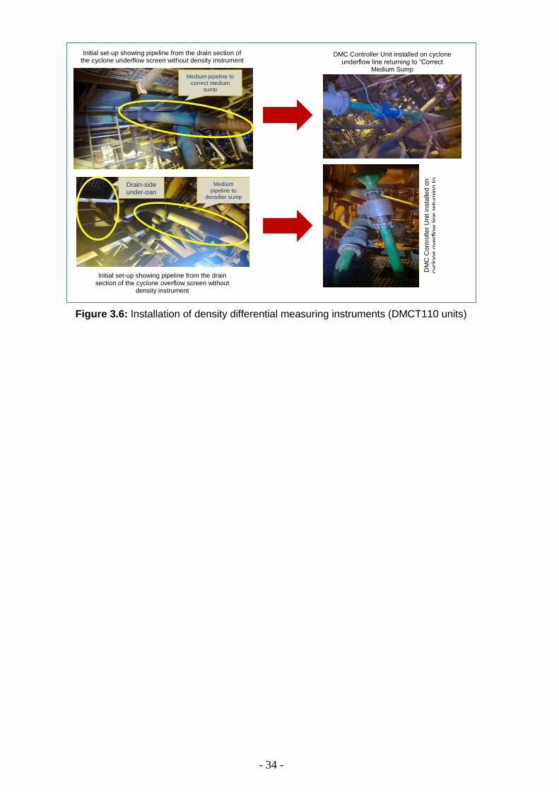
- 34 -

Figure 3.6: Installation of density differential measuring instruments (DMCT110 units)

DMC Controller Unit installed on cyclone underflow line returning to “Correct

Medium Sump

DM

C C

ontr

olle

r U

nit insta

lled o

n

cyclo

ne o

verf

low

lin

e r

etu

rnin

g t

o

Initial set-up showing pipeline from the drain section of the cyclone overflow screen without

density instrument

Drain-side under-pan

Medium pipeline to

densifier sump

Medium pipeline to correct medium

sump

Initial set-up showing pipeline from the drain section of the cyclone underflow screen without density instrument

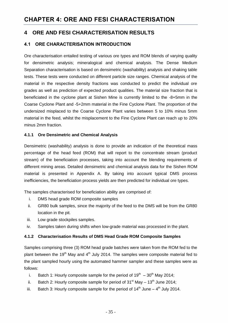
- 35 -

CHAPTER 4: ORE AND FESI CHARACTERISATION

4 ORE AND FESI CHARACTERISATION RESULTS

4.1 ORE CHARACTERISATION INTRODUCTION

Ore characterisation entailed testing of various ore types and ROM blends of varying quality

for densimetric analysis; mineralogical and chemical analysis. The Dense Medium

Separation characterisation is based on densimetric (washability) analysis and shaking table

tests. These tests were conducted on different particle size ranges. Chemical analysis of the

material in the respective density fractions was conducted to predict the individual ore

grades as well as prediction of expected product qualities. The material size fraction that is

beneficiated in the cyclone plant at Sishen Mine is currently limited to the -8+5mm in the

Coarse Cyclone Plant and -5+2mm material in the Fine Cyclone Plant. The proportion of the

undersized misplaced to the Coarse Cyclone Plant varies between 5 to 10% minus 5mm

material in the feed, whilst the misplacement to the Fine Cyclone Plant can reach up to 20%

minus 2mm fraction.

4.1.1 Ore Densimetric and Chemical Analysis

Densimetric (washability) analysis is done to provide an indication of the theoretical mass

percentage of the head feed (ROM) that will report to the concentrate stream (product

stream) of the beneficiation processes, taking into account the blending requirements of

different mining areas. Detailed densimetric and chemical analysis data for the Sishen ROM

material is presented in Appendix A. By taking into account typical DMS process

inefficiencies, the beneficiation process yields are then predicted for individual ore types.

The samples characterised for beneficiation ability are comprised of:

i. DMS head grade ROM composite samples

ii. GR80 bulk samples, since the majority of the feed to the DMS will be from the GR80

location in the pit.

iii. Low grade stockpiles samples.

iv. Samples taken during shifts when low-grade material was processed in the plant.

4.1.2 Characterisation Results of DMS Head Grade ROM Composite Samples

Samples comprising three (3) ROM head grade batches were taken from the ROM fed to the

plant between the 19th May and 4th July 2014. The samples were composite material fed to

the plant sampled hourly using the automated hammer sampler and these samples were as

follows:

i. Batch 1: Hourly composite sample for the period of 19th – 30th May 2014;

ii. Batch 2: Hourly composite sample for period of 31st May – 13th June 2014;

iii. Batch 3: Hourly composite sample for the period of 14th June – 4th July 2014.

- 36 -

Figure 4.1 shows the densimetric profile and chemical analysis of the DMS plant ROM Head

Grade composite samples for the combined size fractions. The results show that the ROM

for all the three batches collected between the 19th May 2014 and 4th July 2014 had relatively

lower proportion of near-density material.

Figure 4.2 shows the chemical analysis of the DMS plant ROM Head Grade composite

samples for the -5+2 mm size fraction of the three batches. The weighted average SiO2

contaminant levels of ROM ranges between 7.3 to 9.4%; while the Fe grade range is 61.0 to

62.3% Fe. Thus, this ROM material can be classified as high-grade ore.

Figure 4.1: Densimetric profile of the DMS head grade ROM samples

Figure 4.2: Chemical quality of the DMS head grade ROM samples

The probability curve in conjunction with the Ecart Probable Moyen was used to demonstrate

the impact of processing efficiency of material with different densimetric profiles. The

Mass %

Fra

ction

Density split (g/cc)

8

2

76

0

78

6

74

4

80

4.0

1.01.36

.0

3.48.2

1.8

1.3

1.6

1.3

73.8

78.7

8.4

6.1

2.4

1.4

1.25

.7

2.3

4.2

1.7

6.5

2.02.4

1.6

1.3

77.7

4.43.0

1.5

3.2 3.8

1.4

3.6 4.6

1.5

Batch 1 Batch 2 Batch 3

%Fe


0

10

20

30

40

50

60

70

0

10

20

30

40

50

60

70

3.6 4.23.2 3.4 4.43.8 4.64.03.0

Batch 3_SiO2Batch 1_SiO2

Batch 2_SiO2Batch 3_Fe

Batch 2_Fe

Batch 1_Fe

%Si

O2

- 37 -

partition curve is determined using the Whitten’s equation as described in Section 2. Each

partition number calculated reflects the fraction of material, per density fraction, that will

report to the cyclone concentrate stream.

The beneficiation ability of the DMS head grade material processed through the DMS plant

during the 19th May 2014 to 4th July 2014 is presented in Figure 4.3. The result indicated the

expected yield for the beneficiation plant operating at cut-density of 3.6 t/m3 with an Ep of

0.17, is 89.78%. When the slimes and -2mm material of the ROM that are fed to thickeners

and Up-current Classifier are also considered, the expected yield from the material is

81.25%. However, the actual plant realised yield for the same period was 79.9%, which is

indicative of inefficiency within the plant. Thus, during this period, the beneficiation plant was

98.3% efficient. With a conservative Ep of 0.17, the current operation practice could not

achieve the required yield, thus necessitating proper control and automation to ensure

stability and good processing efficiency.

When the plant operates at lower EP, such as best practice of 0.05 – 0.10, an improved

performance would be realised with approximately 17 – 19% reduction of the contaminant

levels in the product. Iron ore product with high contaminant levels are not sought after and

results in penalty payment as high as $1.8m/annum. In addition, a 1.5% yield increase in a

plant producing 2.748Mt fine iron ore at a market price of $65/dmt would result in additional

revenue of $2.679m.

Figure 4.3: Effect of ROM’s densimetric profile on yield at cut-density of 3.6 t/m3 and

Ep~0.17

4.1.2.1 Impact of cut-density versus Ep

Ep and cut-density are the important performance factors for the dense medium separation

process. Ep, that is, Ecart probable error measures the deviation of the actual curve from the

ideal curve, with higher Ep indicative of poorer separation. Cut-density is the relative density

corresponding to the 50% of the feed material reporting to either overflow or underflow.

Sensitivity analysis on the effect of Ep and cut-density was applied to the 2014 DMS ROM

0.10.10.30.61.4

5.9

7.5

2.01.41.0

0.60.4

0.1

0.1

0.0

0.1

0.2

0.3

0.4

0.5

0.6

0.7

0.8

0.9

1.0

3

5

7

77

1

76

8

6

4

2

0

4.0 4.2 4.64.43.43.23.0

1.7

3.83.6

76.6

WasteProductPN

Part

itio

n N

um

ber

Mass %

Fra

ction

Density split (g/cc) 77.5

80.0

78.5

81.5

78.0

79.0

81.0

79.5

80.5-1.4

Achieved

Yield

79.9

0

Ideal

Yield

81.2

5

DMS

Plant was

98.3%

Efficient

- 38 -

densimetric profile data. The objective was to evaluate which parameter has the greatest

impact on the expected yield, product grade as well as contaminant levels in the product.

Figure 4.4 shows the effect of Ep and cut-density on the expected product yield and quality

on batch 1 and batch 2. It can be seen by steep slope that the cut-density has the greatest

impact either positive or negative. The graph shows that as the operating Ep increases,

there is a slight increase in expected yield whereas the product Fe-grade decreases.

Furthermore, the graph shows an increase in %SiO2 contaminant as the Ep increases.

The cut-density showed opposite effect to the Ep, where an increase in cut-density would

result in drastic decrease in yield. However, increase in cut-density favours the product

quality thereby increasing the Fe-grade of the product while decreasing the levels of SiO2

contaminant. It can thus be concluded that in order to effect a quick change and response

during beneficiation of iron ore, the metallurgical parameter to manipulate is the cut-density.

Figure 4.4: Predicted yield and quality as function of Ep and cut-density

Densimetric profile of the ROM is influenced by the material composition in the blend, of

which it is summarized in Figure 4.5, whereas detailed daily material class and material

blend is illustrated in Figure 4.6 and Figure 4.7 respectively. The description of the material

type classification for Sishen Mine ores is presented in Appendix A.1 in order to give a

holistic understanding of interpretation linked to material class.

The ROM blend for the period under review is composed mostly of the A-material and the

Bruce-A ore. The A-material is defined as the high grade iron ore which occurs mainly in the

laminated, massive and conglomeratic stratigraphic formations. It also contains gritty iron ore

inter-bedded with shale. Bruce-A is the stockpile with material destined for the DMS plant

DMS ROM COMPOSITION

Yield & Quality Impact as function of Ep & Cut density

DMS ROM Batch 1 (19th – 30th May 2014)

84

86

88

90

92

94

-0.67

0.20.170.130.090.050.01

2.5

3.0

3.5

4.0

4.5

5.0

+0.63

0.20.170.130.090.050.01

-5+2mm

-8+5mm

-25+8mm

-90+25mm

64.5

65.0

65.5

66.0

66.5

67.0

-0.6

0.20.170.130.090.050.01

84

86

88

90

92

94

-5.0

3.83.73.63.53.43.3

64.5

65.0

65.5

66.0

66.5

67.0

+1.6

3.83.73.63.53.43.3

2.5

3.0

3.5

4.0

4.5

5.0

-1.65

3.83.73.63.53.43.3

-5+2mm

-8+5mm

-25+8mm

-90+25mm

Influence of Ep @3.40g/cc Influence of Cut-Density @ Ep ~0.17

Cyclone & @ Ep ~ 0.05 Drum

% Y

ield

Pro

d_%

Fe

Pro

d_%

SiO

2

Pro

d_%

SiO

2

Pro

d_%

Fe

% Y

ield

DMS ROM Batch 2 (31st May – 13th June2014)

87

88

89

90

91

92

93

94

-0.47

0.20.170.130.090.050.01

2.0

2.5

3.0

3.5

4.0

4.5

+0.55

0.20.170.130.090.050.01

-5+2mm

-8+5mm

-25+8mm

-90+25mm

65.0

65.5

66.0

66.5

67.0

67.5

-0.5

0.20.170.130.090.050.01

86

88

90

92

94

3.43.3

-4.7

3.83.73.63.5

65.0

65.5

66.0

66.5

67.0

67.5

+1.5

3.83.73.63.53.43.3

2.0

2.5

3.0

3.5

4.0

4.5

-1.63

3.83.73.63.53.43.3

-8+5mm

-5+2mm-25+8mm

-90+25mm

Influence of Ep @3.40g/ccInfluence of Cut-Density @ Ep ~0.17

Cyclone @Ep~0.05 Drum

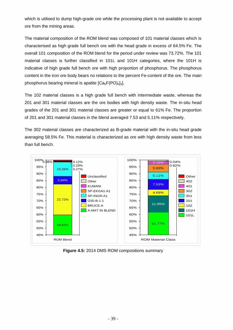
- 39 -

which is utilised to dump high-grade ore while the processing plant is not available to accept

ore from the mining areas.

The material composition of the ROM blend was composed of 101 material classes which is

characterised as high grade full bench ore with the head grade in excess of 64.5% Fe. The

overall 101 composition of the ROM blend for the period under review was 73.72%. The 101

material classes is further classified in 101L and 101H categories, where the 101H is

indicative of high grade full bench ore with high proportion of phosphorus. The phosphorus

content in the iron ore body bears no relations to the percent Fe-content of the ore. The main

phosphorus bearing mineral is apatite [Ca5F(PO)4]3].

The 102 material classes is a high grade full bench with intermediate waste, whereas the

201 and 301 material classes are the ore bodies with high density waste. The in-situ head

grades of the 201 and 301 material classes are greater or equal to 61% Fe. The proportion

of 201 and 301 material classes in the blend averaged 7.53 and 5.11% respectively.

The 302 material classes are characterized as B-grade material with the in-situ head grade

averaging 58.5% Fe. This material is characterized as ore with high density waste from less

than full bench.

Figure 4.5: 2014 DMS ROM compositions summary

45%

55%

50%

60%

65%

100%

95%

90%

85%

80%

75%

70%

5.84%

22.72%

59.63%

0.88%

0.29%

0.27%

0.12%

10.26%

ROM Blend

A-MAT IN BLEND

G50-B-1-1

BRUCE-A

SP-INGR-A1

SP-EKGA1-A1

KUMANI

Other

Unclassified

100%

95%

90%

85%

80%

75%

70%

65%

60%

55%

50%

45%

ROM Material Class

11.95%

4.69%

7.53%

5.11%

5.93%

2.15%0.82%

0.04%

61.77%

101H

102

201

301

302

401

402

Other

101L

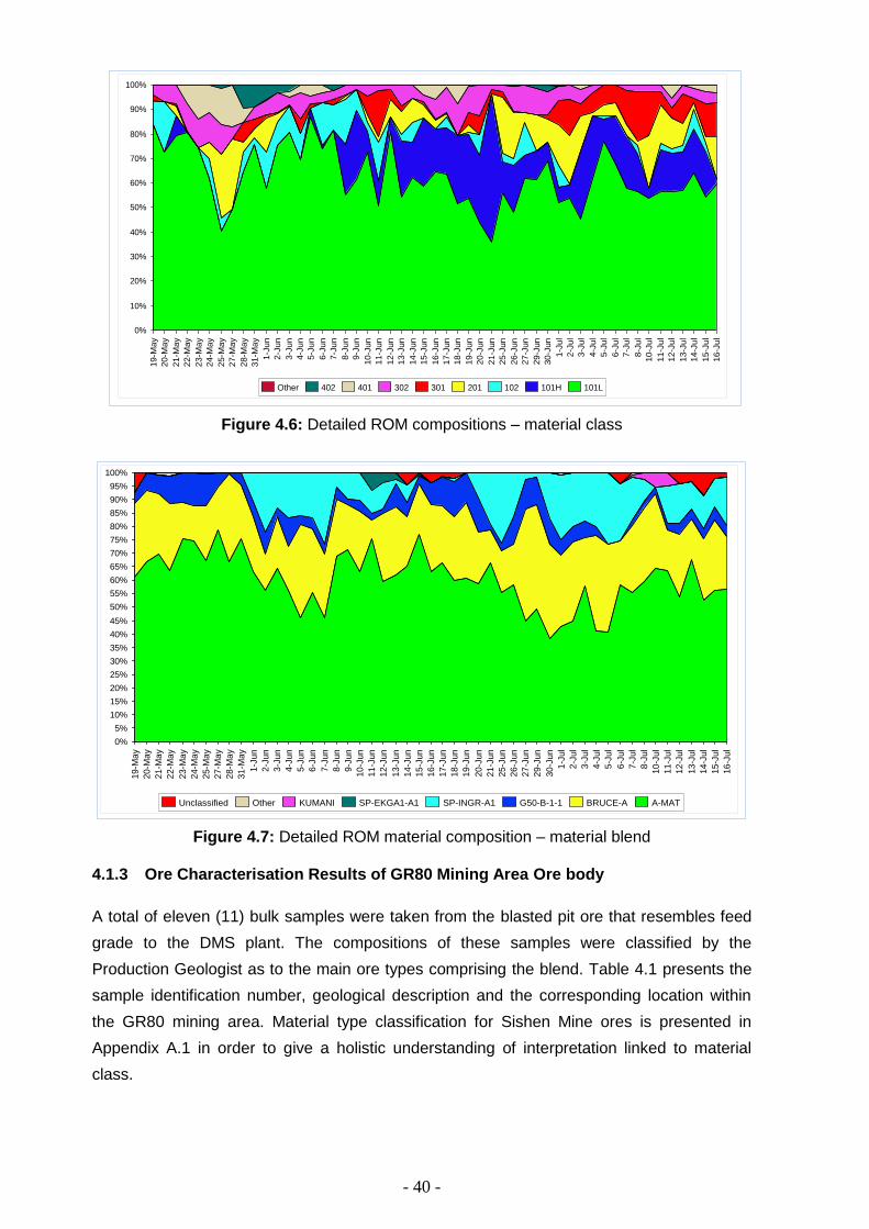
- 40 -

Figure 4.6: Detailed ROM compositions – material class

Figure 4.7: Detailed ROM material composition – material blend

4.1.3 Ore Characterisation Results of GR80 Mining Area Ore body

A total of eleven (11) bulk samples were taken from the blasted pit ore that resembles feed

grade to the DMS plant. The compositions of these samples were classified by the

Production Geologist as to the main ore types comprising the blend. Table 4.1 presents the

sample identification number, geological description and the corresponding location within

the GR80 mining area. Material type classification for Sishen Mine ores is presented in

Appendix A.1 in order to give a holistic understanding of interpretation linked to material

class.

0%

10%

20%

30%

40%

50%

60%

70%

80%

90%

100%

16-J

ul

15-J

ul

15-J

un

14-J

un

13-J

un

12-J

un

11-J

un

10-J

un

9-J

un

14-J

ul

13-J

ul

12-J

ul

11-J

ul

10-J

ul

8-J

ul

7-J

ul

6-J

ul

5-J

ul

4-J

ul

3-J

ul

2-J

ul

1-J

ul

30-J

un

29-J

un

27-J

un

31-M

ay

28-M

ay

27-M

ay

25-M

ay

24-M

ay

23-M

ay

26-J

un

25-J

un

21-J

un

20-J

un

19-J

un

18-J

un

17-J

un

16-J

un

8-J

un

7-J

un

6-J

un

5-J

un

4-J

un

3-J

un

2-J

un

1-J

un

22-M

ay

21-M

ay

20-M

ay

19-M

ay

102 101L101H201301302401402Other

0%

5%

10%

15%

20%

25%

30%

35%

40%

45%

50%

55%

60%

65%

70%

75%

80%

85%

90%

95%

100%

16-J

ul

24-M

ay

21-M

ay

20-M

ay

19-M

ay

25-M

ay

27-M

ay

3-J

un

31-M

ay

1-J

un

28-M

ay

2-J

un

22-M

ay

23-M

ay

4-J

un

10-J

un

5-J

un

6-J

un

9-J

un

7-J

un

8-J

un

14-J

un

15-J

un

13-J

un

12-J

un

11-J

un

20-J

un

29-J

un

16-J

un

26-J

un

17-J

un

19-J

un

30-J

un

27-J

un

25-J

un

18-J

un

21-J

un

15-J

ul

14-J

ul

13-J

ul

12-J

ul

11-J

ul

10-J

ul

8-J

ul

7-J

ul

6-J

ul

3-J

ul

2-J

ul

1-J

ul

5-J

ul

4-J

ul

G50-B-1-1 BRUCE-A A-MATSP-INGR-A1Other SP-EKGA1-A1KUMANIUnclassified

- 41 -

Table 4.1: GR80 bulk samples descriptions

Sample Number Geological Description Sample Number Geological Description

Plant 1 851614A1 HL + BIF (Laminated ore + Banded iron formation)

Plant 7 370422A2 201.1 Laminated ore and Banded iron stone

Plant 2 931614A1 101 EL Laminated ore Plant 8 090419A1 101.1 Laminated ore

Plant 3 231032A1 102.1 Conglomeratic ore Plant 9 851614A2

HL + BIF (Laminated ore + Banded iron formation) Plant 4 851613A2 101.2 EL - Laminated ore

Plant 5 851613A3 201.1 EL+ LY (Laminated ore + banded iron formation)

Plant 10 931614A1 101 EL Laminated ore

Plant 6 1021307A2 301 HL + SH (Laminated + shale)

Plant 11 931614A1 101 EL Laminated ore

Figure 4.8 shows the densimetric analysis results of the combined size fractions, whilst

Appendix A.2 present detailed chemical and densimetric results for GR80 samples. The

results indicated that most of the bulk samples from GR80 area can be classified as

“forgiving” due to relatively low proportion of near density material. However, Plant 1, 7 and 9

samples had relatively higher proportions of the near density and lower density fractions

compared to other ore blends. These samples comprised of class 201 laminated ore with

banded iron formation (BIF). The class 201 ore is characterised as ore with high density BIF.

Figure 4.8: Densimetric analysis of combined GR80 samples

The impact of near density material on the beneficiation efficiency of GR80 material is

demonstrated in Figure 4.9, which compares the processing ability of Plant 1 versus Plant 8

material.

The results indicated that the yield and quality prediction for ROM with high proportion of

near density material would be worse than the ROM with low near density material. It can be

seen in Figure 4.9 that Plant 1 material would produce lower product yield and quality versus

that the Plant 8 material. The predicted yield for Plant 1 and Plant 8 are 85.90% and 95.31%

Mas

s % Fr

actio

n


85

90

65

5

55

95

80

0

75

60

100

10

70

3.63.43.02.8 4.03.2 3.8

Plant 4

Plant 11

Plant 8 Plant 6 Plant 10

Plant 7

Plant 5

Plant 3

Plant 1

Plant 9 Plant 2

- 42 -

respectively, whilst the expected product quality would be 65.25% Fe and 67.76% Fe for

Plant 1 and Plant 8 respectively.

Figure 4.9: Impact of near density material of beneficiation (Plant 1 vs. Plant 8)

Figure 4.10 presents the densimetric profile of the GR80 material at various size fractions.

The graphs show that different size fractions of the same sample have different densimetric

profile. This is the influence of ore liberation of less dense minerals as the ore is crushed to

finer size. Thus, it would be expected that smaller size fraction would have lower yields. This

has been experienced in the processing plant where Fine Cyclone Plant yields are generally

lower than the Coarse Cyclone Plant. The Fine Cyclone Plant treats the -5+2mm material

whereas the Coarse Cyclone Plant treats the -8+5mm material. The -90+8mm material is

treated on the Wemco Drum unit process.

From the data, it can be concluded that the Plant 7 and Plant 9 run-of-mine material would

pose processing challenges in the Cyclone Plant. Table 4.2 shows simulated yield and

product quality when operating at a cut-density of 3.6 t/m3 and Ep of 0.11. These results

show that as the size fraction decrease lower yields are expected as well as lower product

Fe grades. In addition, the contaminants in the product, that is, SiO2 increases with a

decrease in size fraction. Plant 7, which had high proportion of near-density material,

showed the lowest predicted yields and product Fe grade while the SiO2 grade was the

highest of all samples.

2.5 3.15.9

1.3 2.61.3 0.7

0.0

0.30.1

0.0

0.1

0.2

0.3

0.4

0.5

0.6

0.7

0.8

0.9

1.0

8

82

78

0

84

2

4

6

10

80

3.0 3.8

76.7

2.8

3.6

4.03.2

0.9

3.4 3.6

0.9

PN Product Waste

Par

titi

on

Nu

mb

er

PLANT 1

Mas

s %

Fra

ctio

n


0.1

6.9

0.0 0.30.0 0.00.10.0

0.0

0.1

0.2

0.3

0.4

0.5

0.6

0.7

0.8

0.9

1.0100

90

0

10

5

95

3.0

1.9

89.8

3.8 4.03.2 3.4

0.8

3.62.8

PN Product Waste

Par

titi

on

Nu

mb

er

PLANT 8

Mas

s %

Fra

ctio

n


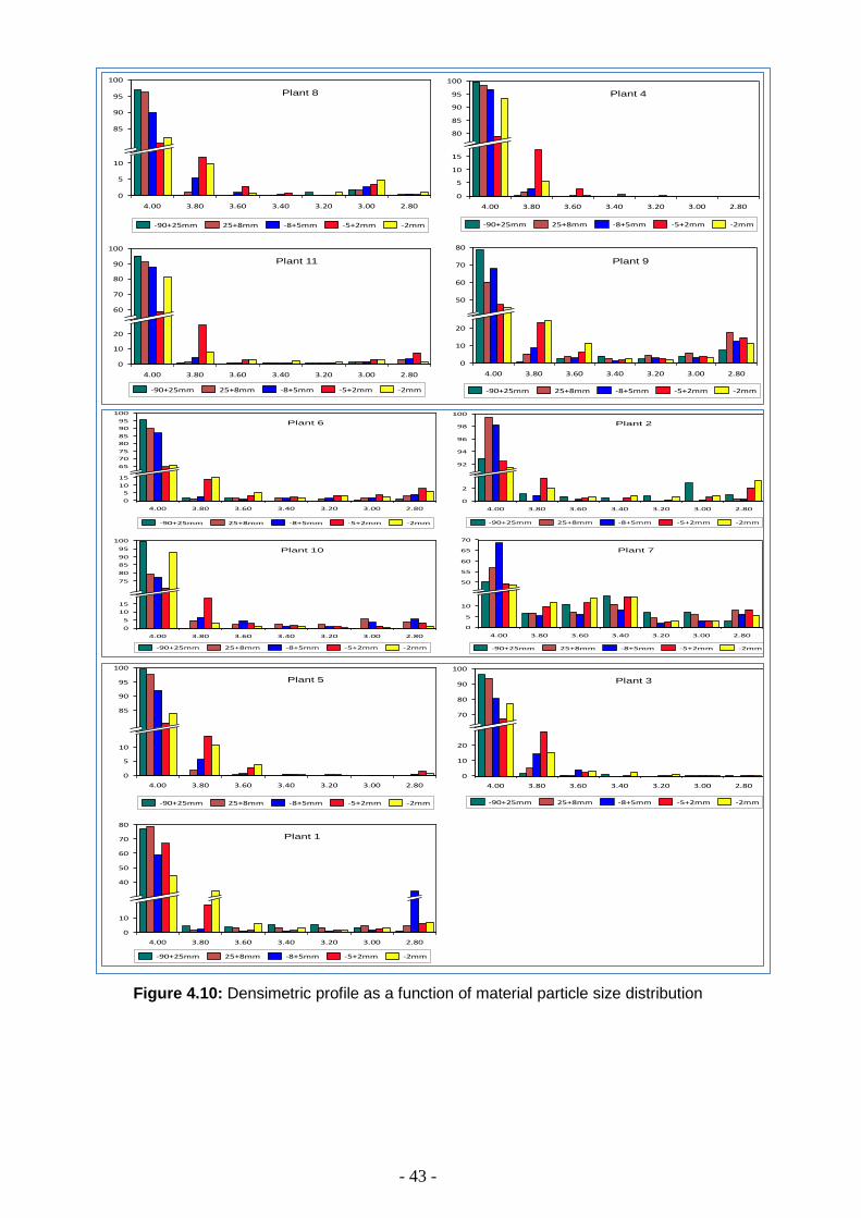
- 43 -

Figure 4.10: Densimetric profile as a function of material particle size distribution

10

85

5

95

90

0

100

3.804.00 3.40 3.003.20 2.803.60

-90+25mm 25+8mm -8+5mm -5+2mm -2mm

20

10

0

100

90

80

70

60

3.203.404.00 3.60 3.003.80 2.80

-2mm-90+25mm -8+5mm -5+2mm25+8mm

Plant 8

Plant 11

50

20

0

60

70

80

10

3.404.00 3.20 3.003.80 2.803.60

-2mm-5+2mm-8+5mm25+8mm-90+25mm

Plant 9

15

5

95

85

80

90

100

10

0

3.204.00 3.603.80 3.40 2.803.00

-90+25mm 25+8mm -8+5mm -2mm-5+2mm

Plant 4

65

70

75

80

100

95

90

85

10

5

0

15

2.803.403.603.804.00 3.003.20

-2mm-5+2mm-8+5mm25+8mm-90+25mm

5

95

75

85

15

100

90

80

10

0

2.803.003.203.403.603.804.00

-2mm-5+2mm-8+5mm25+8mm-90+25mm

Plant 6

Plant 10 65

5

55

70

60

50

10

0

2.803.003.203.403.603.804.00

25+8mm-90+25mm -8+5mm -5+2mm -2mm

Plant 7

100

0

94

98

96

2

92

2.803.20 3.003.403.80 3.604.00

-90+25mm 25+8mm -5+2mm-8+5mm -2mm

Plant 2

100

95

90

85

10

5

0

2.803.003.203.403.603.804.00

-2mm-5+2mm-8+5mm25+8mm-90+25mm

10

0

60

50

80

70

40

2.803.003.204.00 3.80 3.60 3.40

-90+25mm -2mm-5+2mm-8+5mm25+8mm

Plant 5

Plant 1

100

0

70

80

10

90

20

2.803.003.203.403.603.804.00

-5+2mm-90+25mm -8+5mm25+8mm -2mm

Plant 3

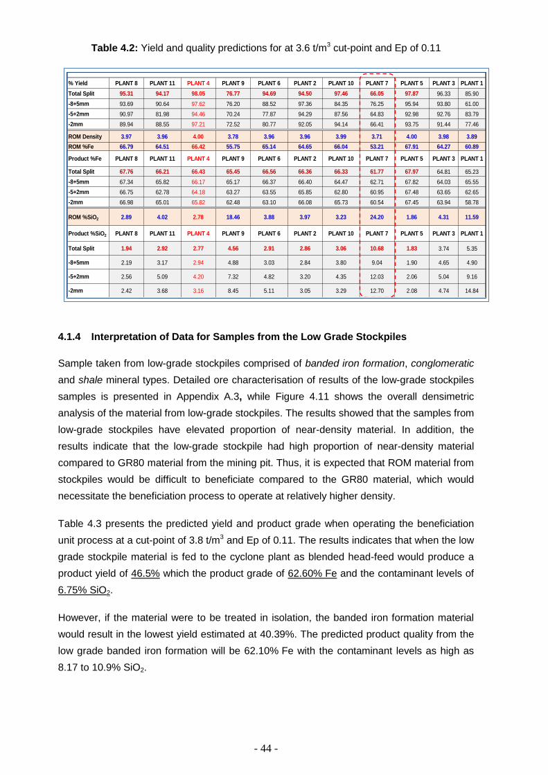
- 44 -

Table 4.2: Yield and quality predictions for at 3.6 t/m3 cut-point and Ep of 0.11

4.1.4 Interpretation of Data for Samples from the Low Grade Stockpiles

Sample taken from low-grade stockpiles comprised of banded iron formation, conglomeratic

and shale mineral types. Detailed ore characterisation of results of the low-grade stockpiles

samples is presented in Appendix A.3, while Figure 4.11 shows the overall densimetric

analysis of the material from low-grade stockpiles. The results showed that the samples from

low-grade stockpiles have elevated proportion of near-density material. In addition, the

results indicate that the low-grade stockpile had high proportion of near-density material

compared to GR80 material from the mining pit. Thus, it is expected that ROM material from

stockpiles would be difficult to beneficiate compared to the GR80 material, which would

necessitate the beneficiation process to operate at relatively higher density.

Table 4.3 presents the predicted yield and product grade when operating the beneficiation

unit process at a cut-point of 3.8 t/m3 and Ep of 0.11. The results indicates that when the low

grade stockpile material is fed to the cyclone plant as blended head-feed would produce a

product yield of 46.5% which the product grade of 62.60% Fe and the contaminant levels of

6.75% SiO2.

However, if the material were to be treated in isolation, the banded iron formation material

would result in the lowest yield estimated at 40.39%. The predicted product quality from the

low grade banded iron formation will be 62.10% Fe with the contaminant levels as high as

8.17 to 10.9% SiO2.

DMS Cut-point

4 Key:

DMS Ep-Value

6

Average Yield ROM (%Fe) Product (%Fe) Product (%SiO2)

94.0% 64.65 66.48 2.90

% Yield PLANT 8 PLANT 11 PLANT 4 PLANT 9 PLANT 6 PLANT 2 PLANT 10 PLANT 7 PLANT 5 PLANT 3 PLANT 1

Total Split 95.31 94.17 98.05 76.77 94.69 94.50 97.46 66.05 97.87 96.33 85.90

-8+5mm 93.69 90.64 97.62 76.20 88.52 97.36 84.35 76.25 95.94 93.80 61.00

-5+2mm 90.97 81.98 94.46 70.24 77.87 94.29 87.56 64.83 92.98 92.76 83.79

-2mm 89.94 88.55 97.21 72.52 80.77 92.05 94.14 66.41 93.75 91.44 77.46

ROM Density 3.97 3.96 4.00 3.78 3.96 3.96 3.99 3.71 4.00 3.98 3.89

ROM %Fe 66.79 64.51 66.42 55.75 65.14 64.65 66.04 53.21 67.91 64.27 60.89

Product %Fe PLANT 8 PLANT 11 PLANT 4 PLANT 9 PLANT 6 PLANT 2 PLANT 10 PLANT 7 PLANT 5 PLANT 3 PLANT 1

Total Split 67.76 66.21 66.43 65.45 66.56 66.36 66.33 61.77 67.97 64.81 65.23

-8+5mm 67.34 65.82 66.17 65.17 66.37 66.40 64.47 62.71 67.82 64.03 65.55

-5+2mm 66.75 62.78 64.18 63.27 63.55 65.85 62.80 60.95 67.48 63.65 62.65

-2mm 66.98 65.01 65.82 62.48 63.10 66.08 65.73 60.54 67.45 63.94 58.78

ROM %SiO2 2.89 4.02 2.78 18.46 3.88 3.97 3.23 24.20 1.86 4.31 11.59

Product %SiO2 PLANT 8 PLANT 11 PLANT 4 PLANT 9 PLANT 6 PLANT 2 PLANT 10 PLANT 7 PLANT 5 PLANT 3 PLANT 1

Total Split 1.94 2.92 2.77 4.56 2.91 2.86 3.06 10.68 1.83 3.74 5.35

-8+5mm 2.19 3.17 2.94 4.88 3.03 2.84 3.80 9.04 1.90 4.65 4.90

-5+2mm 2.56 5.09 4.20 7.32 4.82 3.20 4.35 12.03 2.06 5.04 9.16

-2mm 2.42 3.68 3.16 8.45 5.11 3.05 3.29 12.70 2.08 4.74 14.84

Yield & Quality Based on Densimetric Analysis

Inputs

- 45 -

Figure 4.11: Combined densimetric analysis of samples from low-grade stockpiles

Table 4.3: Yield and product quality predictions for low-grade material at 3.8 t/m3 cut-point

and Ep of 0.11

Figure 4.12 presents the beneficiation potential of different ore types from the low-grade

stockpiles. The results indicated that the shale (SK) ore types would have the highest yields

of 56.98%, followed by the conglomeratic (KGT) ore with 54.29% yields whilst the banded

DMS Cut-point

5 Key:

DMS Ep-Value

6

Average Yield ROM (%Fe) Product (%Fe) Product (%SiO2)

46.5% 52.35 62.60 6.75

Banded Iron FormationBanded Iron

Formation

Banded Iron

Formation

Banded Iron

FormationConglomerate Conglomerate Shale Shale Shale

% Yield BIF G39 BIF 16 BIF 22 BIF 24 KGT 12 KGT 13 SK 7 SK 27 SK 30Combined BIF

Data

Total Split 64.01 57.01 16.63 25.49 44.90 63.09 54.73 61.23 54.58 40.39

-90+25mm

-25+6mm 72.32 64.42 19.00 25.56 50.93 80.32 66.29 70.39 70.67 45.20

-6+2mm 66.87 57.18 16.80 28.88 43.31 69.34 61.70 63.31 55.18 42.70

-2+1mm 38.90 37.93 11.70 19.39 37.18 20.17 26.82 39.98 21.76 25.61

-1mm

ROM Density 4.02 3.84 3.32 3.36 3.71 3.85 3.88 3.93 3.84 3.63

ROM %Fe 55.94 57.71 40.09 45.60 53.33 57.11 57.22 59.70 53.00 50.53

Product %Fe BIF G39 BIF 16 BIF 22 BIF 24 KGT 12 KGT 13 SK 7 SK 27 SK 30Combined BIF

Data

Total Split 62.38 65.64 55.49 58.64 63.31 62.03 64.13 64.88 58.17 62.10

-90+25mm

-25+6mm 61.84 65.64 52.11 57.52 63.85 61.40 63.80 64.50 58.04 61.32

-6+2mm 62.57 65.40 57.96 60.64 64.37 62.70 64.71 65.04 58.52 62.80

-2+1mm 64.37 66.44 61.83 56.73 60.31 63.70 63.40 65.59 57.06 63.22

-1mm

ROM %SiO2 18.80 15.08 24.39 23.31 10.37 8.84 13.02 8.82 10.57 18.92

Product %SiO2 BIF G39 BIF 16 BIF 22 BIF 24 KGT 12 KGT 13 SK 7 SK 27 SK 30Combined BIF

Data

Total Split 8.62 5.06 19.75 15.25 4.74 2.13 5.23 3.68 7.28 9.72

-90+25mm

-25+6mm 9.41 5.20 24.73 17.22 4.20 0.12 5.56 3.98 7.60 10.90

-6+2mm 8.23 5.25 16.11 12.03 4.07 4.89 4.75 3.60 6.82 8.58

-2+1mm 6.10 3.74 10.47 17.86 7.10 4.22 5.57 3.01 7.66 8.17

-1mm

Yield & Quality Based on

Densimetric Analysis

Inputs

Weighted average of all tested samples from low grade stockpiles

Weighted average of

combined BIF

0

5

10

15

20

25

30

35

40

4.84.64.44.24.03.83.63.43.23.02.8

SK 30SK 7

SK 27KGT 13

KGT 12

BIF 24

BIF 22

BIF 16

BIF G39

Total Summary

RD to Sinks (g/cc)

Mas

s Pe

rcen

t

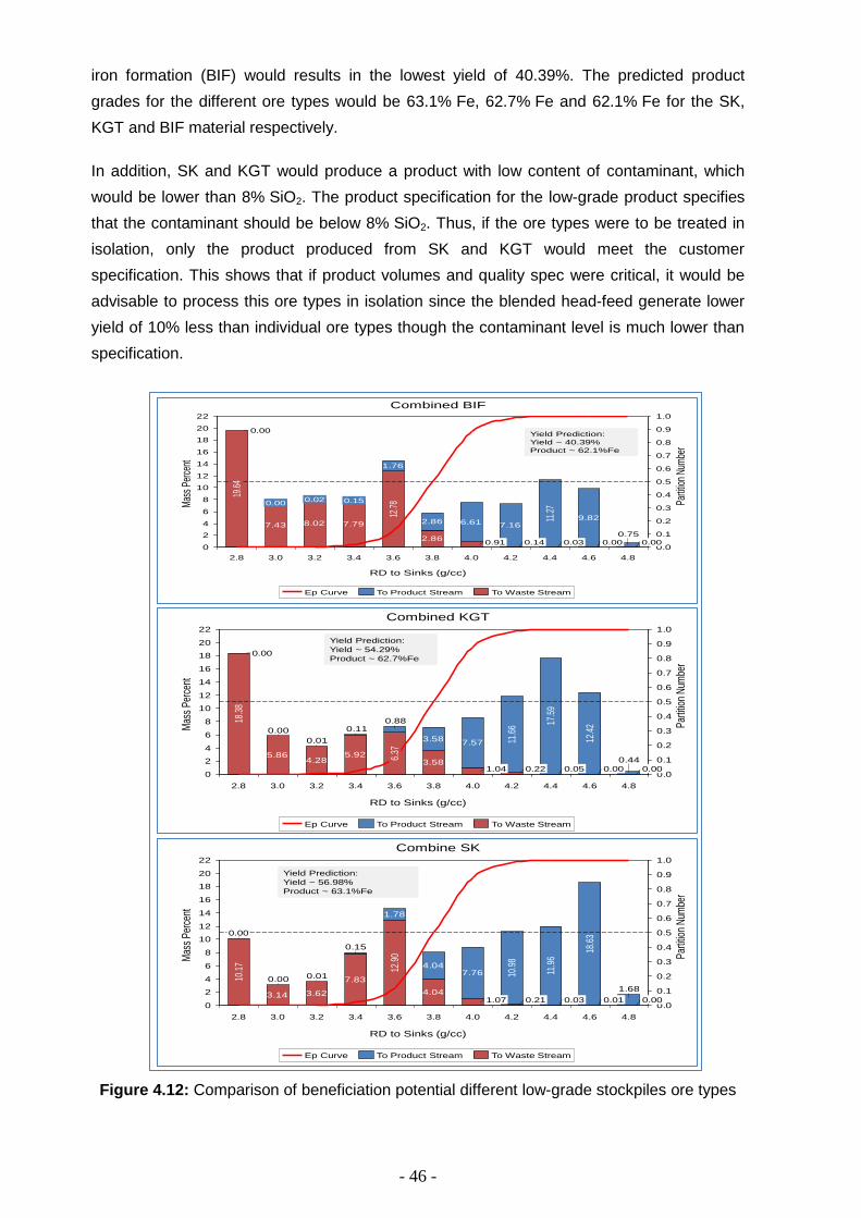
- 46 -

iron formation (BIF) would results in the lowest yield of 40.39%. The predicted product

grades for the different ore types would be 63.1% Fe, 62.7% Fe and 62.1% Fe for the SK,

KGT and BIF material respectively.

In addition, SK and KGT would produce a product with low content of contaminant, which

would be lower than 8% SiO2. The product specification for the low-grade product specifies

that the contaminant should be below 8% SiO2. Thus, if the ore types were to be treated in

isolation, only the product produced from SK and KGT would meet the customer

specification. This shows that if product volumes and quality spec were critical, it would be

advisable to process this ore types in isolation since the blended head-feed generate lower

yield of 10% less than individual ore types though the contaminant level is much lower than

specification.

Figure 4.12: Comparison of beneficiation potential different low-grade stockpiles ore types

Combined BIF

RD to Sinks (g/cc)

Mas

s Pe

rcen

t

8.02 2.867.43 7.79

2.86

1.76

0.75

9.827.166.61

0

2

4

6

8

10

12

14

16

18

20

22

0.0

0.1

0.2

0.3

0.4

0.5

0.6

0.7

0.8

0.9

1.0

19.6

4

3.23.02.8

0.02

0.00

0.00

0.14 0.03

4.84.2 4.64.4

0.91

12.7

80.15

3.4 3.6 3.8 4.0

0.00 0.0011

.27

Ep Curve To Waste StreamTo Product Stream

Parti

tion

Num

ber

Yield Prediction:

Yield ~ 40.39%

Product ~ 62.1%Fe

Combined KGT

RD to Sinks (g/cc)

Mas

s P

erce

nt

3.585.92

4.285.86

0.01

0.110.88

0.00

0.44

7.573.58

0

2

4

6

8

10

12

14

16

18

20

22

0.0

0.1

0.2

0.3

0.4

0.5

0.6

0.7

0.8

0.9

1.0

6.37

3.43.2

18.3

8

0.00

4.83.02.8

0.00

4.6

0.00

12.4

2

4.4

0.05

17.5

9

4.2

0.22

11.6

6

4.0

1.04

3.83.6

To Waste StreamEp Curve To Product Stream

Par

titio

n N

umbe

r

Yield Prediction:

Yield ~ 54.29%

Product ~ 62.7%Fe

Combine SK

RD to Sinks (g/cc)

Mas

s P

erce

nt

4.04

7.83

3.623.14

0.15

0.010.00

1.68

7.764.04

1.78

0

2

4

6

8

10

12

14

16

18

20

22

0.0

0.1

0.2

0.3

0.4

0.5

0.6

0.7

0.8

0.9

1.0

0.01

18.6

3

4.4

0.03

11.9

6

4.2

0.21

4.8

0.00

4.6

10.9

8

4.0

1.07

3.83.6

12.9

0

3.43.23.02.8

10.1

7

0.00

Ep Curve To Waste StreamTo Product Stream

Par

titio

n N

umbe

r

Yield Prediction:

Yield ~ 56.98%

Product ~ 63.1%Fe

- 47 -

4.1.5 Interpretation of Data for Samples from the Actual Pilot Plant Processing

Samples comprising the product, waste and feed were taken for the material that was

processed through the Ultra-High Density DMS (UHDMS) Pilot Plant. The samples

processed though UHDMS comprised of two set of samples, that is, (i) material from low-

grade stockpiles and (ii) waste material from the JIG plant. Tabulated data of the densimetric

material from these samples is presented in Appendix A.4, while graphical presentation of

the data is depicted in Figure 4.13. The material from low-grade stockpile showed as similar

densimetric profile while the JIG waste material was characterised with high proportion of

low-density material. However, similar Fe grade can be seen for the same density splits for

all samples tested.

Figure 4.13: Densimetric profile of feed material processed through UHDMS

The theoretical prediction of the expected yield and product grade for the low-grade stockpile

and JIG waste material is presented in Figure 4.14. The low-grade material had a weighted

ROM grade of 49.34%Fe whereas the JIG waste material has a ROM grade of 43.58% Fe.

The predicted yields where 57.59% and 44.19% for the low grade stockpile Jig waste

material respectively, whereas their respective product quality is estimated as 64.6% Fe and

64.8% Fe.

0

5

10

15

20

25

30

35

40

4,69

24,73

4,72

4,23

5,03

4,42

38,41

5,77

4,15 7,3

0 12,12

9,05

21,40

18,53

13,8617

,41

5,43

6,28

3.63.4 4.0 4.2 4.4 4.6 4.8 5.03.8

3,20

12,45

8,91 12,55

25,69

8,313,1

8

8,29

9,91

Jig Waste (15/01/2014)Low Grade (14/01/2014 Day Shift)

Low Grade (14/01/2014 Night Shift)

RD to Sinks (g/cc)

Ore Mass Distribution as function of Density Split

Mas

s (%

)

- 48 -

Figure 4.14: Yield and product grade prediction (a) Low-grade stockpile (b) Jig discard

Figure 4.15 presents the comparison of the “observed partition curve” versus the “theoretical

predicted partition curve”. The “observed partition curve” is constructed using the low-grade

stockpile material. The density of the circulating medium was set at density of 4.00 t/m3 in

order to give an expected cut-point of 4.20 t/m3. However, the results for the cut-points while

processing low-grade material during the day shift and night shift operation were 4.51 t/m3

and 4.44 t/m3 respectively. Coarse ferrosilicon was used for preparation of the heavy dense

medium, thus the high offset (i.e. cut-point shift) might be related to relatively high-density

differentials that were measured during material processing. The achieved yield was

averaging 54.5% with product grade of higher than 66.11% Fe. The yield was 3.09% lower

than the predicted yield whilst the product quality was 1.51% higher than prediction. Thus,

producing a product with higher product quality would be expected to have a negative impact

on yield.

(a)

(b)

Mas

s Pe

rcen

t

Low Grade Stockpile Predictions

RD to Sinks (g/cc)

25.7

3.2 4.6 3.7 3.6

3.6 8.7

17.1 18.5

9.0

0.00.00.31.2

0.50.1

0

5

10

15

20

25

30

0.0

0.1

0.2

0.3

0.4

0.5

0.6

0.7

0.8

0.9

1.0

0.0

0.0

5.04.84.64.0 4.44.23.83.63.4

To Waste StreamTo Product Stream Pred. Partition

Parti

tion

Num

ber

Predictions

• Feed: 49.34%Fe

• Yield: 57.59%

• Product: 64.6%Fe

Mas

s P

erce

nt

Jig Waste Material

RD to Sinks (g/cc)

38.4

4.4 5.12.5

7.812.3 12.4

8.3

0.00.00.21.12.5

0.7

0

5

10

15

20

25

30

35

40

0.0

0.1

0.2

0.3

0.4

0.5

0.6

0.7

0.8

0.9

1.0

5.04.83.8

4.10.1

3.6

0.0

3.4

0.0

4.64.44.24.0

To Product Stream Pred. PartitionTo Waste Stream

Par

titio

n N

umbe

r

Predictions

• Feed: 43.58%Fe

• Yield: 44.19%

• Product: 64.8%Fe

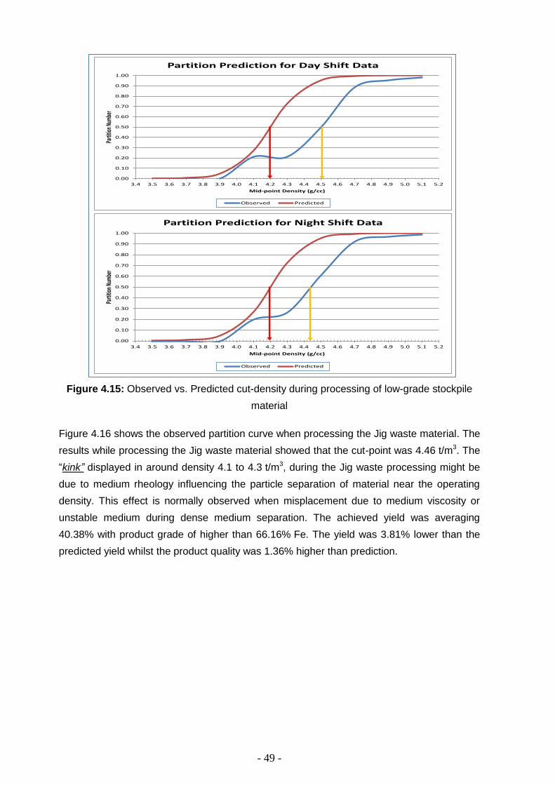
- 49 -

Figure 4.15: Observed vs. Predicted cut-density during processing of low-grade stockpile

material

Figure 4.16 shows the observed partition curve when processing the Jig waste material. The

results while processing the Jig waste material showed that the cut-point was 4.46 t/m3. The

“kink” displayed in around density 4.1 to 4.3 t/m3, during the Jig waste processing might be

due to medium rheology influencing the particle separation of material near the operating

density. This effect is normally observed when misplacement due to medium viscosity or

unstable medium during dense medium separation. The achieved yield was averaging

40.38% with product grade of higher than 66.16% Fe. The yield was 3.81% lower than the

predicted yield whilst the product quality was 1.36% higher than prediction.

0.00

0.10

0.20

0.30

0.40

0.50

0.60

0.70

0.80

0.90

1.00

3.4 3.5 3.6 3.7 3.8 3.9 4.0 4.1 4.2 4.3 4.4 4.5 4.6 4.7 4.8 4.9 5.0 5.1 5.2

Parti

tion N

umbe

r

Mid-point Density (g/cc)

Partition Prediction for Day Shift Data

Observed Predicted

0.00

0.10

0.20

0.30

0.40

0.50

0.60

0.70

0.80

0.90

1.00

3.4 3.5 3.6 3.7 3.8 3.9 4.0 4.1 4.2 4.3 4.4 4.5 4.6 4.7 4.8 4.9 5.0 5.1 5.2

Parti

tion N

umbe

r


Partition Prediction for Night Shift Data

Observed Predicted

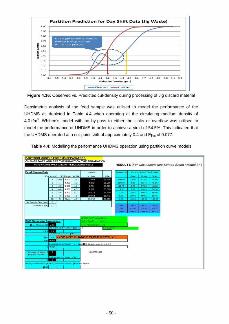
- 50 -

Figure 4.16: Observed vs. Predicted cut-density during processing of Jig discard material

Densimetric analysis of the feed sample was utilised to model the performance of the

UHDMS as depicted in Table 4.4 when operating at the circulating medium density of

4.0 t/m3. Whitten’s model with no by-pass to either the sinks or overflow was utilised to

model the performance of UHDMS in order to achieve a yield of 54.5%. This indicated that

the UHDMS operated at a cut-point shift of approximately 0.4 and Epm of 0.077.

Table 4.4: Modelling the performance UHDMS operation using partition curve models

PARTITION MODELS FOR DMS SEPARATORS

CHANGE DATA AND SEE THE IMPACT ON THE SEPARATION

RESULTS (For calculations see Spread Sheet <Model 3> )

Feed Stream Data mass% Partition % Cum %Density Distribution

SG Class # SG Range Av SG in class %Fe Feed Floats Sinks

1 Float 4.000 3.9 33.063 21.418 100.00 33.06 87.56 45.50

2 4 4.200 4.1 4.872 51.300 100.00 4.87 92.44 45.50

3 4.2 4.400 4.3 6.754 55.699 80.70 6.75 97.89 46.80

4 4.4 4.600 4.5 9.042 60.500 19.30 9.04 99.63 54.10

5 4.6 4.800 4.7 15.514 64.400 1.35 15.51 99.84 69.40

6 4.8 5.000 4.9 20.063 66.772 0.08 20.06 99.86 89.45

10 5 Sink 4.3 10.692 68.439 1.35 10.69 100.00 100.00

Av Particle Size (mm) 3

Feed rate (tph) 100 TPH 100.0 45.5 54.5

SG 4.158 3.630 4.732

%Fe 49.52 30.59 65.32

MODEL for Partition Curve

DMS Separator Parameters R(x) = Rc(x)(1 b) + b

ρm = Medium SG 4.00 Rc(x) =1/(1+(exp(λ(x-1))]

Cut Point Shift = CPS = ρ50 - ρm λ = 1.099/Ic

CPS 0.4cut density = ρcut = ρ50

ρ50 4.4 <<DO NOT CHANGE THIS DIRECTLY !!epm 0.077

Corrected imperfection = Ic = epm/ρ50 {Realistic range 0.4 to 0.01)}

Ic 0.017

by-pass to floats: b 0 0.097381407

by-pass to sinks: 0

fluid recovery to sinks = Rf

Rf 0

Density Differential = ρdiff = ρunderflow medium - ρoverflow medium

ρdiff

NOTE: CHANGE ONLY DATA IN THE BLACKENED CELLS

0.00

0.10

0.20

0.30

0.40

0.50

0.60

0.70

0.80

0.90

1.00

3.4 3.5 3.6 3.7 3.8 3.9 4.0 4.1 4.2 4.3 4.4 4.5 4.6 4.7 4.8 4.9 5.0 5.1 5.2

Parti

tion

Num

ber


Partition Prediction for Day Shift Data (Jig Waste)

Observed Predicted

kink might be due to medium rhelogy & misplacement within unit process

- 51 -

4.1.6 Summary of Ore Characterisation and Processing Results

The summary of the weighted average densimetric profile for the GR80, Low-grade

stockpile material and 2014 DMS ROM are shown in Figure 4.17:

GR80 and 2014 DMS ROM comprises very low near-density material.

Low-grade stockpiles comprise a high proportion of near-density material.

The 2014 DMS ROM shows an increase in low-density material in the feed

compared to GR80. This can be seen from a higher proportion of 2.8 t/m3

material for 2014 DMS ROM (i.e. 5.8%) compared to 1.78% for the GR80 ore

body.

Figure 4.17: Summary of densimetric analysis for the GR80 vs. Low-grade vs. 2014 DMS

ROM samples

In spite of increased low-density material in the 2014 DMS ROM, this material is

characterised as having low near-density material and thus easy to beneficiate in the

dense medium process.

The densimetric analysis of the GR80 material show that the high-grade ore from the

mining area has low proportion of near-density material and can be classified as

“forgiving” and easy to beneficiate. This material will produce high yields when

processed through the dense medium beneficiation circuit. In addition, qualities

expected from these samples would be high, that is, 65.2% Fe.

Characterisation of the low-grade stockpiles indicated that the material from these

stockpiles is characterised by elevated proportions of near-density material. Thus, in

order to beneficiate these material relatively high operating densities are required for

the dense medium separation process. However, these material can be beneficiated

0

90

80

25

5

15

30

10

75

20

85

1.7

8

2.0

6

2.0

6

15

.85

1.2

8 16

.02

14

.29

1.7

2

14

.81

5.8

0

1.6

9

1.7

1

86

.55

1.7

1

1.7

7

13

.00

4.003.803.60

89

.37

3.203.002.80

13

.94

1.2

0

12

.10

1.3

0

3.40

GR80 vs. Low Grade vs. 2014 ROM

RD to Sinks (g/cc)

Ma

ss P

erc

en

t

Low Grade Material

GR80 Samples

2014 Composite ROM

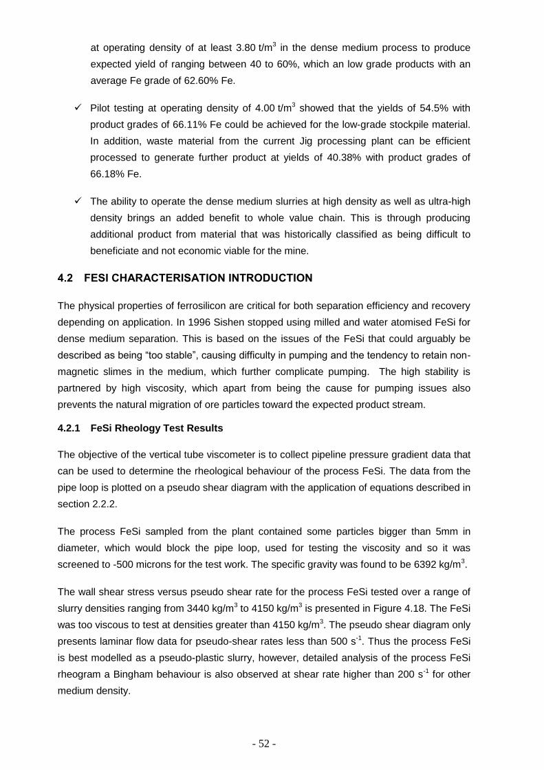
- 52 -

at operating density of at least 3.80 t/m3 in the dense medium process to produce

expected yield of ranging between 40 to 60%, which an low grade products with an

average Fe grade of 62.60% Fe.

Pilot testing at operating density of 4.00 t/m3 showed that the yields of 54.5% with

product grades of 66.11% Fe could be achieved for the low-grade stockpile material.

In addition, waste material from the current Jig processing plant can be efficient

processed to generate further product at yields of 40.38% with product grades of

66.18% Fe.

The ability to operate the dense medium slurries at high density as well as ultra-high

density brings an added benefit to whole value chain. This is through producing

additional product from material that was historically classified as being difficult to

beneficiate and not economic viable for the mine.

4.2 FESI CHARACTERISATION INTRODUCTION

The physical properties of ferrosilicon are critical for both separation efficiency and recovery

depending on application. In 1996 Sishen stopped using milled and water atomised FeSi for

dense medium separation. This is based on the issues of the FeSi that could arguably be

described as being “too stable”, causing difficulty in pumping and the tendency to retain non-

magnetic slimes in the medium, which further complicate pumping. The high stability is

partnered by high viscosity, which apart from being the cause for pumping issues also

prevents the natural migration of ore particles toward the expected product stream.

4.2.1 FeSi Rheology Test Results

The objective of the vertical tube viscometer is to collect pipeline pressure gradient data that

can be used to determine the rheological behaviour of the process FeSi. The data from the

pipe loop is plotted on a pseudo shear diagram with the application of equations described in

section 2.2.2.

The process FeSi sampled from the plant contained some particles bigger than 5mm in

diameter, which would block the pipe loop, used for testing the viscosity and so it was

screened to -500 microns for the test work. The specific gravity was found to be 6392 kg/m3.

The wall shear stress versus pseudo shear rate for the process FeSi tested over a range of

slurry densities ranging from 3440 kg/m3 to 4150 kg/m3 is presented in Figure 4.18. The FeSi

was too viscous to test at densities greater than 4150 kg/m3. The pseudo shear diagram only

presents laminar flow data for pseudo-shear rates less than 500 s-1. Thus the process FeSi

is best modelled as a pseudo-plastic slurry, however, detailed analysis of the process FeSi

rheogram a Bingham behaviour is also observed at shear rate higher than 200 s-1 for other

medium density.

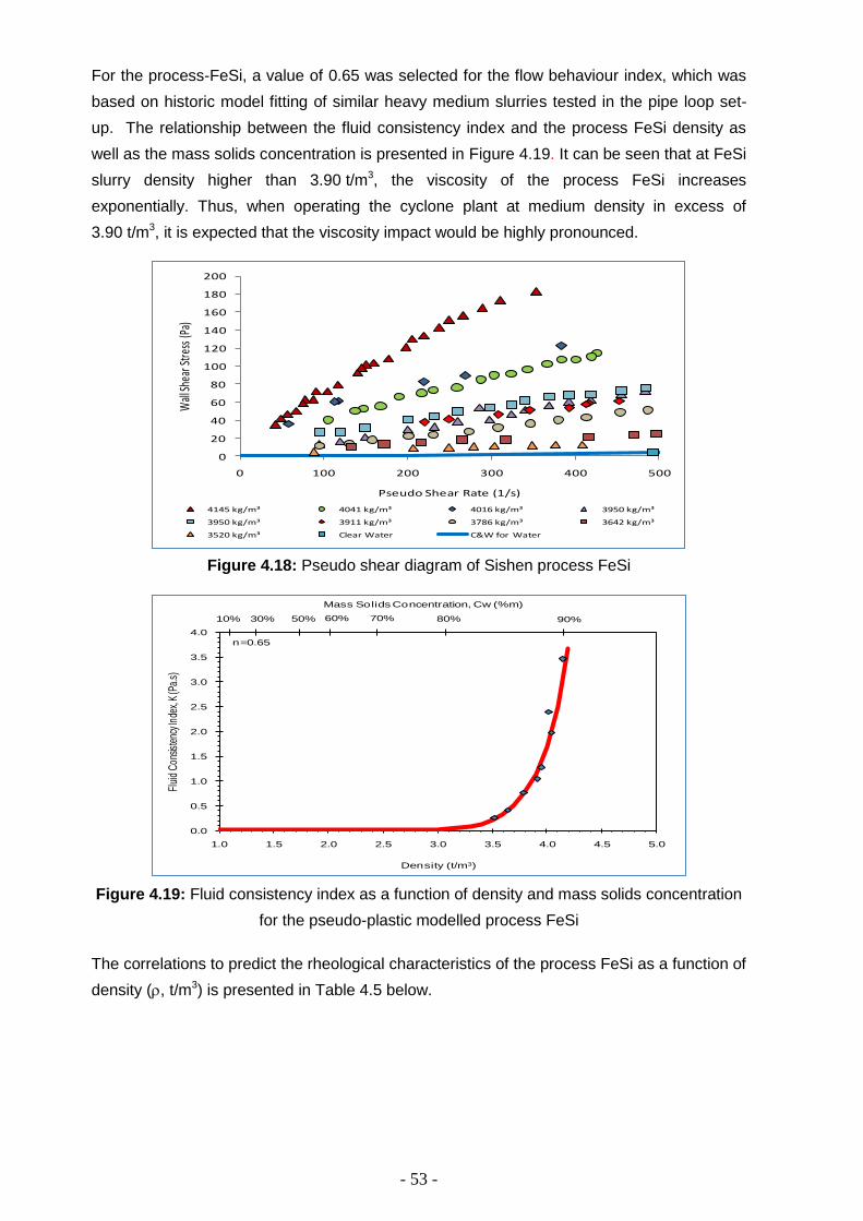
- 53 -

For the process-FeSi, a value of 0.65 was selected for the flow behaviour index, which was

based on historic model fitting of similar heavy medium slurries tested in the pipe loop set-

up. The relationship between the fluid consistency index and the process FeSi density as

well as the mass solids concentration is presented in Figure 4.19. It can be seen that at FeSi

slurry density higher than 3.90 t/m3, the viscosity of the process FeSi increases

exponentially. Thus, when operating the cyclone plant at medium density in excess of

3.90 t/m3, it is expected that the viscosity impact would be highly pronounced.

Figure 4.18: Pseudo shear diagram of Sishen process FeSi

Figure 4.19: Fluid consistency index as a function of density and mass solids concentration

for the pseudo-plastic modelled process FeSi

The correlations to predict the rheological characteristics of the process FeSi as a function of

density (, t/m3) is presented in Table 4.5 below.

0

20

40

60

80

100

120

140

160

180

200

0 100 200 300 400 500

Wall

Shea

r Stre

ss (P

a)

Pseudo Shear Rate (1/s)

4145 kg/m³ 4041 kg/m³ 4016 kg/m³ 3950 kg/m³

3950 kg/m³ 3911 kg/m³ 3786 kg/m³ 3642 kg/m³

3520 kg/m³ Clear Water C&W for Water

0.0

0.5

1.0

1.5

2.0

2.5

3.0

3.5

4.0

1.0 1.5 2.0 2.5 3.0 3.5 4.0 4.5 5.0

Flui

d C

onsis

tenc

y Ind

ex, K

(Pa.

s)

Density (t/m3).

10% 30% 50% 70% 80% 90%60%

Mass Solids Concentration, Cw (%m)

n=0.65

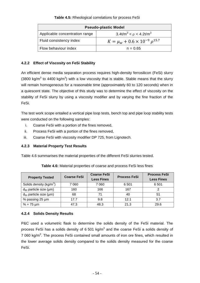
- 54 -

Table 4.5: Rheological correlations for process FeSi

Pseudo-plastic Model

Applicable concentration range 3.4t/m3 < < 4.2t/m3

Fluid consistency index 𝐾 = 𝜇𝑤 + 0.6 × 10−9 𝜌15.7

Flow behaviour index n = 0.65

4.2.2 Effect of Viscosity on FeSi Stability

An efficient dense media separation process requires high-density ferrosilicon (FeSi) slurry

(3800 kg/m3 to 4400 kg/m3) with a low viscosity that is stable. Stable means that the slurry

will remain homogeneous for a reasonable time (approximately 60 to 120 seconds) when in

a quiescent state. The objective of this study was to determine the effect of viscosity on the

stability of FeSi slurry by using a viscosity modifier and by varying the fine fraction of the

FeSi.

The test work scope entailed a vertical pipe loop tests, bench top and pipe loop stability tests

were conducted on the following samples:

i. Coarse FeSi with a portion of the fines removed,

ii. Process FeSi with a portion of the fines removed,

iii. Coarse FeSi with viscosity modifier DP 725, from Lignotech.

4.2.3 Material Property Test Results

Table 4.6 summarises the material properties of the different FeSi slurries tested.

Table 4.6: Material properties of coarse and process FeSi less fines

Property Tested Coarse FeSi Coarse FeSi

Less Fines Process FeSi

Process FeSi

Less Fines

Solids density (kg/m3) 7 060 7 060 6 501 6 501

d90 particle size (µm) 160 166 167 2

d50 particle size (µm) 68 71 40 51

% passing 25 µm 17.7 9.8 12.1 3.7

% + 75 µm 47.3 48.3 21.3 29.6

4.2.4 Solids Density Results

P&C used a volumetric flask to determine the solids density of the FeSi material. The

process FeSi has a solids density of 6 501 kg/m3 and the coarse FeSi a solids density of

7 060 kg/m3. The process FeSi contained small amounts of iron ore fines, which resulted in

the lower average solids density compared to the solids density measured for the coarse

FeSi.

- 55 -

Figure 4.20 and Figure 4.21 below shows the relationship between slurry densities, solids

mass concentration and solids volume concentration for the coarse FeSi and process FeSi

respectively.

Figure 4.20: m, Cw, s and Cv relationship for the coarse FeSi

Figure 4.21: m, Cw, s and Cv relationship for the process FeSi

4.2.5 Particle Size Analysis

Detailed particle size distribution of the coarse FeSi and process FeSi less fines were

measured by wet sieving is presented in Appendix B.2. In order to quantify the difference

observed in the size distribution, the measured data was fitted to a Rosin-Rammler model

(equations 3.1 and 3.2) as described in section 3.2 of this document.

Figure 4.22 presents the Rosin-Rammler regression for the coarse FeSi with and without

fines measured using the wet sieving method. The Dn fitting parameter of the coarse FeSi

and coarse FeSi less fines were 229.32 and 442.5 respectively, whilst the n parameter were

0.967 and 0.829 respectively.

10% 30% 50% 60% 70% 80% 90%

0%

10%

20%

30%

40%

50%

60%

1 000 1 500 2 000 2 500 3 000 3 500 4 000 4 500 5 000

Mixture Density, m (kg/m3)

Mass Solids Concentration, Cw

Ss = 7060 kg/m³

Cv = 46.5%

Volu

met

ric S

olid

s C

once

ntra

tion,

Cv

Cw = 86.0%

3820 kg/m³m=

10% 30% 50% 60% 70% 80% 90%

0%

10%

20%

30%

40%

50%

60%

1 000 1 500 2 000 2 500 3 000 3 500 4 000 4 500 5 000

Mixture Density, m (kg/m3)

Mass Solids Concentration, Cw

Ss = 6501 kg/m³

Cv = 48.6%

Volu

met

ric S

olid

s C

once

ntra

tion,

Cv

Cw = 86.0%

3673 kg/m³m=

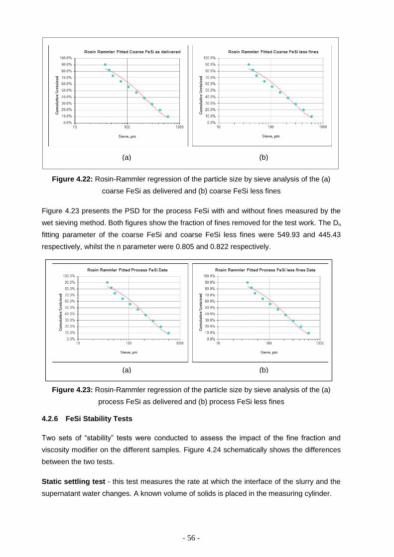
- 56 -

Figure 4.22: Rosin-Rammler regression of the particle size by sieve analysis of the (a)

coarse FeSi as delivered and (b) coarse FeSi less fines

Figure 4.23 presents the PSD for the process FeSi with and without fines measured by the

wet sieving method. Both figures show the fraction of fines removed for the test work. The Dn

fitting parameter of the coarse FeSi and coarse FeSi less fines were 549.93 and 445.43

respectively, whilst the n parameter were 0.805 and 0.822 respectively.

Figure 4.23: Rosin-Rammler regression of the particle size by sieve analysis of the (a)

process FeSi as delivered and (b) process FeSi less fines

4.2.6 FeSi Stability Tests

Two sets of “stability” tests were conducted to assess the impact of the fine fraction and

viscosity modifier on the different samples. Figure 4.24 schematically shows the differences

between the two tests.

Static settling test - this test measures the rate at which the interface of the slurry and the

supernatant water changes. A known volume of solids is placed in the measuring cylinder.

(a) (b)

(a) (b)

- 57 -

Vertical pipe settling test - this test measures the density of the suspended medium as a

function over time in a 2 m high column of slurry. It provides an indication of the rate at which

solids settle out of the slurry suspension.

Figure 4.24: Comparison of the two types of settling tests and results

4.2.6.1 Stability Test No 1: Static Settling Test Results

The aim of the static bench top settling tests provides an indication of the rate at which

surface water separates from the solids for a given slurry mixture. The medium with high

settling rate is regarded as unstable and thus expected have lower viscosity.

Figure 4.25 shows the Coarse FeSi less fines settling rate decreases (becomes more stable)

with an increase in slurry density. At low densities, the initial settling rate is high as solids

separate quickly, and at high densities, the settling rate decreases, shown by the slope of

the initial data points. Figure 4.26 also shows that the Process FeSi less fines settling rate

decreases with an increase in density. Figure 4.27 show that the coarse FeSi with viscosity

modifier settles in a very similar manner to the coarse FeSi fewer fines.

STATIC SETTLING TEST

H1 H2 H3

time = 0 time =d t

VERTICAL PIPE SETTLING TEST

Pressure Pressure Pressure

Transmitter Transmitter Transmitter

ms 1 ms2 ms 3

Pressure Pressure Pressure

Transmitter Transmitter Transmitter

time = 0 time =d t

ms Density of suspended medium

suspended medium

settled bed of solids

clear supernatant water

time = final t

time = final t

0

50

100

150

200

250

Inte

rfa

ce

he

ight

(mm

)

Time (minutes)

H3H1 H2

0 dt final t

0

500

1000

1500

2000

2500

3000

3500

4000

4500

5000

De

nsity

of

Susp

end

ed

Me

diu

m,

m

s(k

g/m

3)

Time (minutes)

0 dt final t

ms1

ms3

ms2

- 58 -

Figure 4.25: Bench top settling tests for coarse FeSi less fines

Figure 4.26: Bench top settling tests for process FeSi less fines

Figure 4.27: Bench top settling tests for coarse FeSi with viscosity modifier

0

50

100

150

200

250

0 5 10 15 20 25 30

Inte

rface

hei

ght (

mm

)

Time (minutes)

3600 kg/m³ 3800 kg/m³ 4000 kg/m³ 4200 kg/m³

0

50

100

150

200

250

0 5 10 15 20 25 30

Inte

rface

hei

ght (

mm

)

Time (minutes)

3600 kg/m³ 3800 kg/m³ 3900 kg/m³ 4000 kg/m³

0

50

100

150

200

250

0 5 10 15 20 25 30

Inte

rface

hei

ght (

mm

)

Time (minutes)

3600 kg/m³ 3800 kg/m³ 4000 kg/m³ 4200 kg/m³

High settling rate

Low settling rate

- 59 -

To summarise the results, Figure 4.28 shows a comparison of the bench top test results for

different FeSi samples at a density of approximately 4000 kg/m3. From the data, it can be

seen that the Coarse FeSi settles fastest with the viscosity modifier added. With the fines

removed, it settles slightly faster than the coarse FeSi sample. The process FeSi less fines

also settles slightly faster than the full process FeSi sample.

Figure 4.28: Comparison of bench top settling test results at a density of 4000 kg/m3

4.2.6.2 Stability Test No 2: Vertical Pipe Settling Tests

The pipe loop settling tests provide an indication of the rate at which the FeSi mixture

density changes while at rest in a vertical pipe. The rate at which the FeSi mixture density

changes is an indication of the rate at which a solid bed of FeSi particles settles out of the

slurry, forming a self-supporting structure in the slurry. Conversely, it can be considered a

measure of rate of settled bed formation. The test records the density of the suspended

medium as a function over time.

Appendix B.3 presents detailed test results of vertical pipe settling tests whilst Figure 4.29

Figure 4.30, Figure 4.31 and Figure 4.32 show plots of density of suspended medium versus

time for “coarse less fines”, “process FeSi”, “process FeSi less fines” and “coarse FeSi with

viscosity modifier” respectively over ten minutes. The first minute is of particular significance

as the residence time of FeSi slurry in the DMS drum and cyclone was determined as 58

seconds for Sishen operation. However, in the first few minutes of this test the slurry is

forming a bed between the closed valve and the bottom pressure transmitter during which

time the density remains almost constant. After this, as the bed is formed in the pipe section

between the pressure transmitters, the change in density of suspended medium with time

shows a constant settling rate in the pipe. All of these tests, if continued long enough reach a

constant density of that of water. This is when all the FeSi particles have settled out of the

slurry and are supporting each other by direct particle-particle contact; analogous to a stack

0

50

100

150

200

250

0 5 10 15 20 25 30

Inte

rface

hei

ght (

mm

)

Time (minutes)

Coarse FeSi Coarse FeSi less Fines

Coarse FeSi with Rheology Modifier Process FeSi Less Fines

Process FeSi

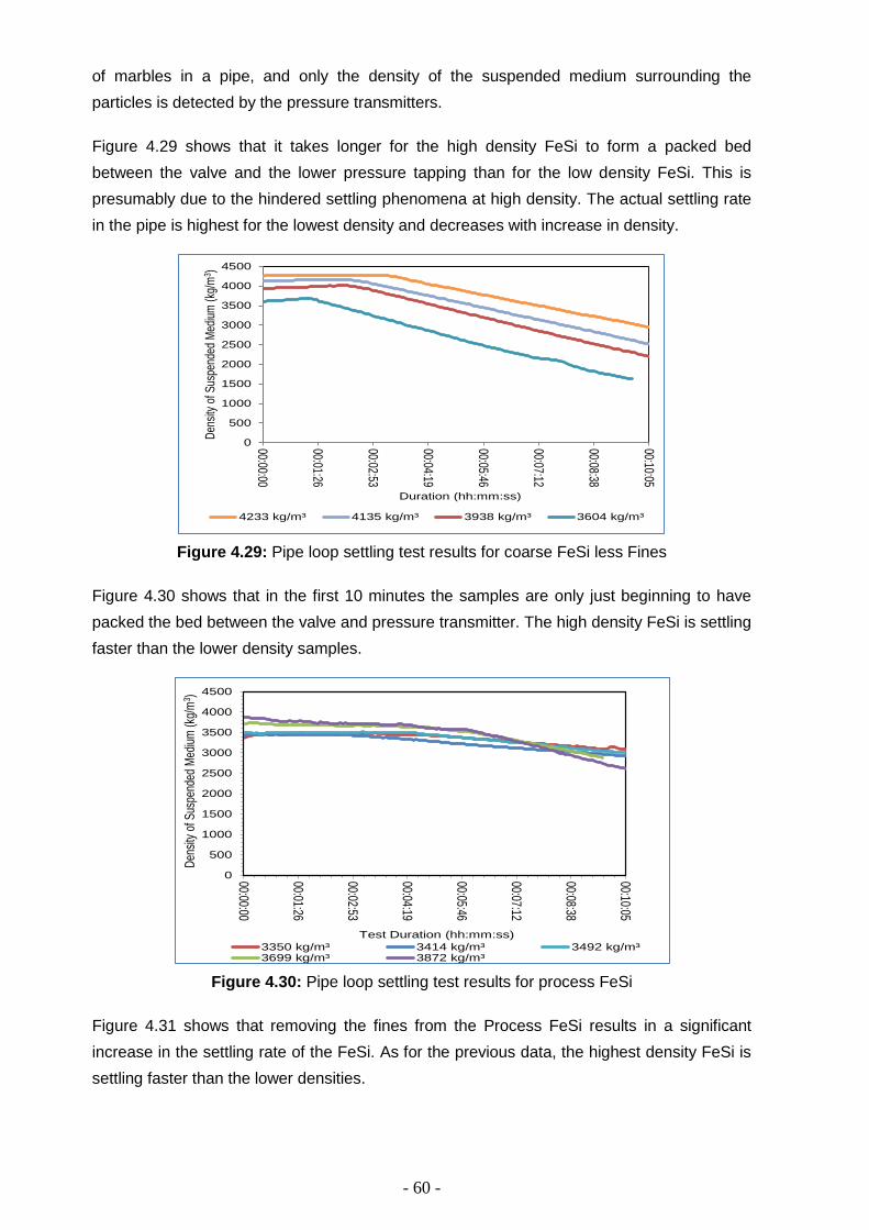
- 60 -

of marbles in a pipe, and only the density of the suspended medium surrounding the

particles is detected by the pressure transmitters.

Figure 4.29 shows that it takes longer for the high density FeSi to form a packed bed

between the valve and the lower pressure tapping than for the low density FeSi. This is

presumably due to the hindered settling phenomena at high density. The actual settling rate

in the pipe is highest for the lowest density and decreases with increase in density.

Figure 4.29: Pipe loop settling test results for coarse FeSi less Fines

Figure 4.30 shows that in the first 10 minutes the samples are only just beginning to have

packed the bed between the valve and pressure transmitter. The high density FeSi is settling

faster than the lower density samples.

Figure 4.30: Pipe loop settling test results for process FeSi

Figure 4.31 shows that removing the fines from the Process FeSi results in a significant

increase in the settling rate of the FeSi. As for the previous data, the highest density FeSi is

settling faster than the lower densities.

0

500

1000

1500

2000

2500

3000

3500

4000

4500

00:00:00

00:01:26

00:02:53

00:04:19

00:05:46

00:07:12

00:08:38

00:10:05D

ensi

ty o

f Sus

pend

ed M

ediu

m (k

g/m

3 )

Duration (hh:mm:ss)

4233 kg/m³ 4135 kg/m³ 3938 kg/m³ 3604 kg/m³

0

500

1000

1500

2000

2500

3000

3500

4000

4500

00:00:00

00:01:26

00:02:53

00:04:19

00:05:46

00:07:12

00:08:38

00:10:05

Den

sity

of S

uspe

nded

Med

ium

(kg/

m3 )

Test Duration (hh:mm:ss)

3350 kg/m³ 3414 kg/m³ 3492 kg/m³3699 kg/m³ 3872 kg/m³

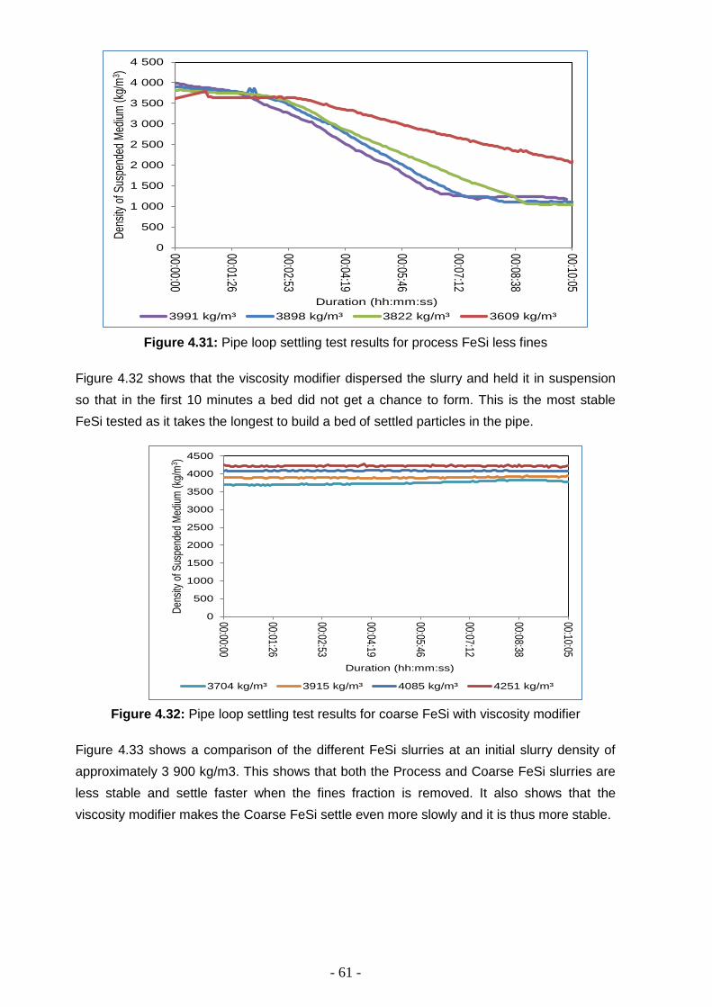
- 61 -

Figure 4.31: Pipe loop settling test results for process FeSi less fines

Figure 4.32 shows that the viscosity modifier dispersed the slurry and held it in suspension

so that in the first 10 minutes a bed did not get a chance to form. This is the most stable

FeSi tested as it takes the longest to build a bed of settled particles in the pipe.

Figure 4.32: Pipe loop settling test results for coarse FeSi with viscosity modifier

Figure 4.33 shows a comparison of the different FeSi slurries at an initial slurry density of

approximately 3 900 kg/m3. This shows that both the Process and Coarse FeSi slurries are

less stable and settle faster when the fines fraction is removed. It also shows that the

viscosity modifier makes the Coarse FeSi settle even more slowly and it is thus more stable.

0

500

1 000

1 500

2 000

2 500

3 000

3 500

4 000

4 500

00:00:00

00:01:26

00:02:53

00:04:19

00:05:46

00:07:12

00:08:38

00:10:05

Den

sity

of S

uspe

nded

Med

ium

(kg/

m3 )

Duration (hh:mm:ss)

3991 kg/m³ 3898 kg/m³ 3822 kg/m³ 3609 kg/m³

0

500

1000

1500

2000

2500

3000

3500

4000

4500

00:00:00

00:01:26

00:02:53

00:04:19

00:05:46

00:07:12

00:08:38

00:10:05

Den

sity

of S

uspe

nded

Med

ium

(kg

/m3 )

Duration (hh:mm:ss)

3704 kg/m³ 3915 kg/m³ 4085 kg/m³ 4251 kg/m³

- 62 -

Figure 4.33: Pipe loop settling test results at slurry density of approximately 3900 kg/m3

4.2.7 Comparison of Static and Vertical Pipe Settling Test Results

Table 4.7 shows a comparison of the results of the two different sets of settling tests. The

static settling test measures the rate at which the interface of the slurry and the supernatant

water changes. The vertical pipe-settling test measures the rate at which the slurry settles

into a bed of solids supporting each other and thereby “settling out” of the slurry.

Table 4.7: Comparison of FeSi settling test results

Sample Static Settling Test Vertical Pipe Settling Test

Coarse FeSi 3 4

Coarse FeSi less fines 2 2

Coarse FeSi with viscosity

modifier

1 5

Process FeSi 5 3

Process FeSi less fines 4 1

Where 1 = settles fastest; 5 = settles slowest

For the Dense Medium Separator it is desirable to have a FeSi that remains suspended as

long as possible. For the FeSi samples tested this is the coarse FeSi with viscosity modifier

as the FeSi particles form a settled bed more slowly in that sample than in any of the others,

in other words they stay suspended in the water for longer. However, it is the fastest settling

(i.e. least stable) in the bench top settling test.

The vertical pipe settling test shows an interesting trend in that all the coarse FeSi samples

show hindered settling as the settling rate decreases with increase in density. Conversely,

the process FeSi samples show an increased settling rate as density increases. This trend

was not evident in the static settling tests that all settled slower as the density increased.

0

500

1000

1500

2000

2500

3000

3500

4000

4500

00:00:00

00:01:26

00:02:53

00:04:19

00:05:46

00:07:12

00:08:38

00:10:05

Dens

ity o

s Su

spen

ded

Med

ium

(kg/

m3 )

Test Duration (hh:mm:ss)

Coarse FeSi Coarse less fines

Process FeSi Process less fines

Coarse + rheology modifier

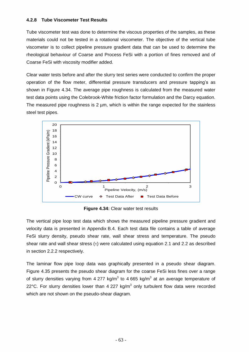
- 63 -

4.2.8 Tube Viscometer Test Results

Tube viscometer test was done to determine the viscous properties of the samples, as these

materials could not be tested in a rotational viscometer. The objective of the vertical tube

viscometer is to collect pipeline pressure gradient data that can be used to determine the

rheological behaviour of Coarse and Process FeSi with a portion of fines removed and of

Coarse FeSi with viscosity modifier added.

Clear water tests before and after the slurry test series were conducted to confirm the proper

operation of the flow meter, differential pressure transducers and pressure tapping’s as

shown in Figure 4.34. The average pipe roughness is calculated from the measured water

test data points using the Colebrook-White friction factor formulation and the Darcy equation.

The measured pipe roughness is 2 µm, which is within the range expected for the stainless

steel test pipes.

Figure 4.34: Clear water test results

The vertical pipe loop test data which shows the measured pipeline pressure gradient and

velocity data is presented in Appendix B.4. Each test data file contains a table of average

FeSi slurry density, pseudo shear rate, wall shear stress and temperature. The pseudo

shear rate and wall shear stress () were calculated using equation 2.1 and 2.2 as described

in section 2.2.2 respectively.

The laminar flow pipe loop data was graphically presented in a pseudo shear diagram.

Figure 4.35 presents the pseudo shear diagram for the coarse FeSi less fines over a range

of slurry densities varying from 4 277 kg/m3 to 4 665 kg/m3 at an average temperature of

22°C. For slurry densities lower than 4 227 kg/m3 only turbulent flow data were recorded

which are not shown on the pseudo-shear diagram.

0

2

4

6

8

10

12

14

16

18

20

0 1 2 3

Pip

elin

e P

ress

ure

Gra

dien

t (kP

a/m

)

Pipeline Velocity, (m/s)

CW curve Test Data After Test Data Before

- 64 -

Figure 4.35: Pseudo shear diagram of coarse FeSi less fines

Figure 4.36 presents a pseudo shear diagram for the process FeSi less fines at slurry

densities ranging from 3 670 kg/m3 to 3 994 kg/m3 at an average temperature of 29.5°C.

Figure 4.36: Pseudo shear diagram for process FeSi less fines

Figure 4.37, Figure 4.38 and Figure 4.39 depict a comparison between process FeSi and

process FeSi less fines at densities of approximately 3900, 3800 and 3660 kg/m3

respectively.

0

20

40

60

80

100

120

0 100 200 300 400 500 600

Wal

l She

ar S

tress

(Pa)


4277 kg/m³ 4373 kg/m³ 4462 kg/m³ 4568 kg/m³

4625 kg/m³ 4665 kg/m³ Water

0

10

20

30

40

50

60

70

80

90

100

0 100 200 300 400 500 600

Wal

l She

ar S

tress

(Pa)


3670 kg/m³ 3812 kg/m³ 3910 kg/m³


- 65 -

Figure 4.37: Pseudo shear diagram comparing process FeSi to process FeSi less fines at

approximately 3900 kg/m3





High density coarse FeSi slurry was circulated in the vertical pipe loop in laminar flow and

viscosity modifier was gradually added until a ten percent drop in pressure gradient was

0

20

40

60

80

100

0 100 200 300 400 500 600

Wal

l She

ar S

tres

s (P

a)


Process FeSi 3903 kg/m³ Process FeSi less Fines at 3910 kg/m³

0

10

20

30

40

50

60

70

80

90

100

0 100 200 300 400 500 600

Wal

l She

ar S

tress

(Pa)



0

10

20

30

40

50

60

70

80

90

100

0 100 200 300 400 500 600

Wal

l She

ar S

tress

(Pa)



- 66 -

measured in the laminar flow region. The amount of dry FeSi in the loop was determined and

the dose of 100 ml per dry tonne of FeSi was determined as a suitable dose of viscosity

modifier to test. Figure 4.40 shows the pseudo shear diagrams of coarse FeSi with 100ml

viscosity modifier per dry tonne of FeSi over a range of densities from 3947 kg/m3 to 4500

kg/m3. The tests were conducted at an average temperature of 22.8°C.

Figure 4.40: Pseudo shear diagram of coarse FeSi with viscosity modifier added

Figure 4.41, Figure 4.42 and Figure 4.43 show pseudo shear diagrams of coarse FeSi with

and without viscosity modifier at densities of 4500 kg/m3, 4260 kg/m3 and 3980 kg/m3

respectively. The test data shows that the viscosity modifier decreases the flow curve of the

coarse FeSi at a dose of 100ml per dry tonne. The change in flow behaviour is more

pronounced for the higher density tests.

Figure 4.41: Pseudo shear diagram of coarse FeSi at a density of approximately 4500 kg/m3

with and without viscosity modifier added

0

10

20

30

40

50

60

0 200 400 600 800 1000

Wal

l She

ar S

tress

(Pa)


4500 kg/m³ 4357 kg/m³ 4262 kg/m³ 4170 kg/m³


0

10

20

30

40

50

60

70

80

0 200 400 600 800 1000

Wal

l She

ar S

tress

(Pa)


Coarse FeSi at 4506 kg/m³ Coarse FeSi + rheology modifier at 4503 kg/m³

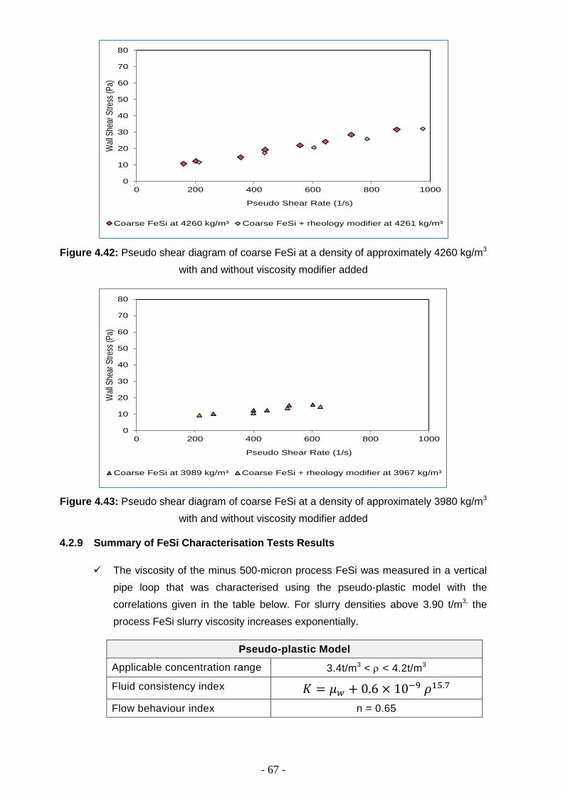
- 67 -





4.2.9 Summary of FeSi Characterisation Tests Results

The viscosity of the minus 500-micron process FeSi was measured in a vertical

pipe loop that was characterised using the pseudo-plastic model with the

correlations given in the table below. For slurry densities above 3.90 t/m3, the

process FeSi slurry viscosity increases exponentially.

Pseudo-plastic Model

Applicable concentration range 3.4t/m3 < < 4.2t/m3

Fluid consistency index 𝐾 = 𝜇𝑤 + 0.6 × 10−9 𝜌15.7

Flow behaviour index n = 0.65

0

10

20

30

40

50

60

70

80

0 200 400 600 800 1000

Wal

l She

ar S

tress

(Pa)



0

10

20

30

40

50

60

70

80

0 200 400 600 800 1000

Wal

l She

ar S

tress

(Pa)



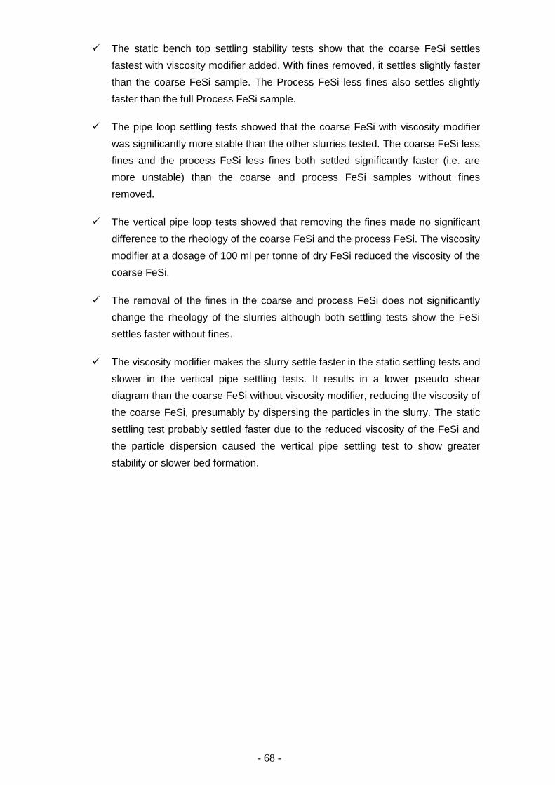
- 68 -

The static bench top settling stability tests show that the coarse FeSi settles

fastest with viscosity modifier added. With fines removed, it settles slightly faster

than the coarse FeSi sample. The Process FeSi less fines also settles slightly

faster than the full Process FeSi sample.

The pipe loop settling tests showed that the coarse FeSi with viscosity modifier

was significantly more stable than the other slurries tested. The coarse FeSi less

fines and the process FeSi less fines both settled significantly faster (i.e. are

more unstable) than the coarse and process FeSi samples without fines

removed.

The vertical pipe loop tests showed that removing the fines made no significant

difference to the rheology of the coarse FeSi and the process FeSi. The viscosity

modifier at a dosage of 100 ml per tonne of dry FeSi reduced the viscosity of the

coarse FeSi.

The removal of the fines in the coarse and process FeSi does not significantly

change the rheology of the slurries although both settling tests show the FeSi

settles faster without fines.

The viscosity modifier makes the slurry settle faster in the static settling tests and

slower in the vertical pipe settling tests. It results in a lower pseudo shear

diagram than the coarse FeSi without viscosity modifier, reducing the viscosity of

the coarse FeSi, presumably by dispersing the particles in the slurry. The static

settling test probably settled faster due to the reduced viscosity of the FeSi and

the particle dispersion caused the vertical pipe settling test to show greater

stability or slower bed formation.

- 69 -

CHAPTER 5: CYCLONE PLANT AUTOMATION AND CONTROL

5 AUTOMATION AND CONTROL INTRODUCTION

Sishen DMS plant process produces approximately 25% of the product through the cyclone

plant, with yields ranging from 70% to 80%. A tighter control philosophy can improve yield

consistency by 5%, which would deliver at least 1.25% additional product to Sishen. This

type of statement is made on the basis that cyclone setup and operation throughout all

mineral industries is in a relatively poor shape. This is due to any number of reasons such

as:

(i) Incorrectly specified system setup

(ii) Overfeeding

(iii) Variation in viscosity

(iv) System changes over time

(v) Poor maintenance

Therefore, consistent system management, measurement and insight is required to

maximize the opportunity that the cyclones present. Through the use of modelling and

simulation, the aim was to identify the financial benefit to be gained from better operation,

and consequently, trade this off against the costs associated with operation. Moreover, it has

helped in identifying how much effort should be placed on this part of the operation.

The main aim of the automation of the cyclone modules is aimed at maintaining the process

stability thereby improving the metallurgical efficiency during the beneficiation of iron ore

material. This is premised on the fact that, as the head grade of ROM declines, the level of

near-density material increases thereby required the dense medium beneficiation circuit

operating at optimum efficiency relating to Ep values within best practice range of between

0.02 – 0.05.

The operational objectives of the automated control of dense media system for the cyclone

plant are called upon to: (i) ensuring stability of process, (ii) suppressing the influence of

external disturbances, and (iii) optimizing the economic performance of the cyclone plant,

that is, minimize yield losses to waste.

Thus, the automation focuses on maintaining the following process parameters:

a) Dense medium in the correct and dilute medium sumps level is controlled to a

minimum of 25%.

b) Correct medium flow rate to be controlled at an absolute minimum of 150 m3/h.

c) Maintaining the medium to ore (M:O) ratio at a minimum levels of 5:1.

d) Ensure sufficient cyclone inlet pressure as well as maintaining the variation in

pressure differential between cyclone clusters to below 10%.

e) Monitor and control the cyclone density differential to within the 0.02 – 0.05 range.

- 70 -

Based on current and past conditions, a soft sensor will be used to identify possible problem

areas in the near future. This information will then be communicated to the operators and

advice given on action steps to take to avoid problems occurring. This soft sensor will thus

be employed to act as a pro-active decision management tool.

The expected solution of the control is to ensure that the feed to a particular module is

interlocked to the FeSi medium condition. Thus, interlocking correct medium flow with the

module ore feed rate will ensure that minimum medium-to-ore (M:O) ratio is maintained.

(Petersen, 2010) in addition (Mukherjee, et al., 2003) indicated that the stability of the dense

medium cyclone system can be monitored through the inlet pressure measurement. Thus,

one of the primary objectives of the automated control is maintaining cyclone inlet pressure

across all operating cyclones constant. The monitoring of cyclone inlet pressure would

indicate that a constant head is maintained across cyclone cluster as well as indication of

system imbalances and the blockages. Should there be a constant increase in pressure

differential between cyclones in a cluster (e.g. 5100 cyclones) or P between clusters of a

particular module (e.g. 5100 vs. 5200 set), then the system should warn the control room

operator than a particular module is not in balance. Corrective action might be manual flow

balance through the “Jacko-Sleeve” valves or unblocking the blocked feed line.

Figure 5.1 shows the flow sheet for the automated module and indicates the critical

measuring instruments that have been installed.

- 71 -

Figure 5.1: General module layout of with instruments for monitoring and control (Tom,

2014)

- 72 -

5.1 AUTOMATED MODULE VERSUS TRADITIONAL MODULE

The current cyclone plant set-up is manual operation, with only automated control being for

the medium density. This section aim to indicate the traditional un-instrumented module with

the instrumented module to satisfy what is termed level 1 & 2 regulatory controls in terms of

layers of controls. Typical layers of control are presented in Figure 5.2 below.

Figure 5.2: Generic layer of controls (de Villiers, et al., 2014)

Automation of the cyclone plant module involved installation of the followings instruments:

(i) Acoustic level indicators for the monitoring and control of both correct and dilute

media sumps. This is critical to ensure enough medium is maintained in the sump to

ensure correct flow to the beneficiation cyclone as well as feed to the magnetic

separation stream

(ii) Non-contact, SONARtrac flowmeters for the measurement of the medium flow rates

to the cyclone circuit. This is required in order to determine the medium-to-ore ratio

for the module. SONARtrac monitoring systems do not utilize ultrasonic; they

employ patented sonar array processing techniques to listen to, and interpret, flow

turbulence and sound fields generated by the machinery, piping and process flow.

This passive listening approach results in measurement of the flow rate and amount

of entrained air/gas with a high degree of accuracy and repeatability.

(iii) Non-contact SONARtrac flowmeter for the measurement of the mixture of ore and

dense medium after mixing box to ensure constant flow is maintained between

cyclone clusters. This was preferred as the new mixing box similar to Venetia mine

would require major structural change and thus impractical for the current set-up.

Layers of Control

Enterprise Wide Control / Optimization (LP Models)

OEM Drives / Conveyors / Crusher Rail Car

Autonomous TrucksCrusher Unit Control (

SCADA / PLC)Load Out Control

Dynamic Dispatch System Crusher Circuit MPC Dispatch Scheduler

Fleet Management System Plant Wide Controller Logistics Controller

L1

1ms

L2

100ms

L3

30sec –

30min

L4

30min –

8hrs

L5

days -

months

Mining Process / Plant Logistics

Instruments / Devices / Equipment – Equip ILocks & Alarms– ASM Eq

uip

me

nt

Pro

tect

ion

Pro

cess

Sa

fety

/

Sta

bili

ty

Sta

bili

ty / U

nit

Op

timiz

atio

n

Op

timiz

atio

n /

Sch

ed

ulin

gL

on

g T

erm

Pla

nn

ing

Regulatory Control (PID / Sequences / ARC) - Process ILocks & Alarms – S88, ASM

Soft Sensors & Advanced Control (Fuzzy / MBC / MPC)

Real Time Optimization and Scheduling

MES / MIS & Dynamic Simulation

- 73 -

(iv) Cyclone in-let pressure transmitters for all cyclones in the cyclone-cluster.

Figure 5.3, Figure 5.4 and Figure 5.5 show the instruments installed in cyclone module as

part of the automation project, which includes sump level indicator, non-contact medium

flowmeter, cyclone inlet-pressure transmitters and cyclone cluster balance respectively.

Figure 5.3: Sump level indicators

Figure 5.4: Cyclone inlet pressure transmitter

Dense medium sump without a level controller

Dense medium sump with a level controller

Hawk Sultan Acoustic Wave Level Sensor

Correct

Medium Sump

Cyclone cluster without inlet pressure monitor

Cyclo

ne c

luste

r w

ith

inle

t pre

ssure

tr

ansm

itte

rs

VEGABAR82 Pressure

transmitter

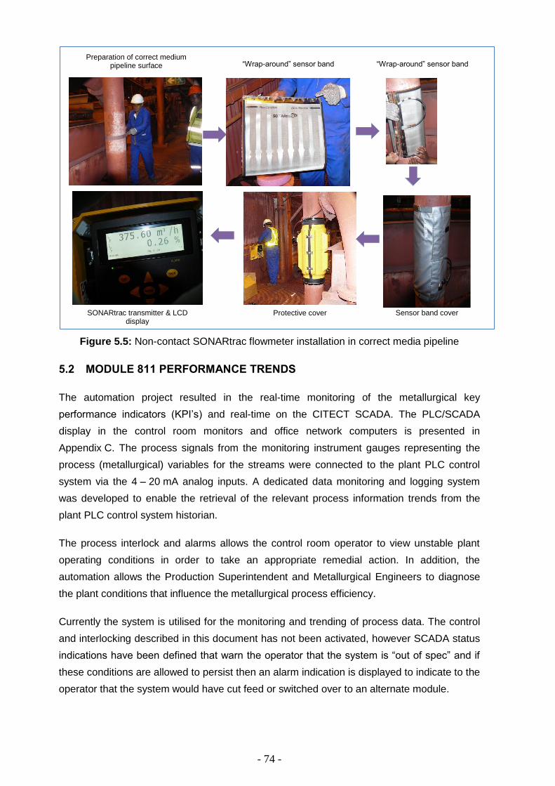
- 74 -

Figure 5.5: Non-contact SONARtrac flowmeter installation in correct media pipeline

5.2 MODULE 811 PERFORMANCE TRENDS

The automation project resulted in the real-time monitoring of the metallurgical key

performance indicators (KPI’s) and real-time on the CITECT SCADA. The PLC/SCADA

display in the control room monitors and office network computers is presented in

Appendix C. The process signals from the monitoring instrument gauges representing the

process (metallurgical) variables for the streams were connected to the plant PLC control

system via the 4 – 20 mA analog inputs. A dedicated data monitoring and logging system

was developed to enable the retrieval of the relevant process information trends from the

plant PLC control system historian.

The process interlock and alarms allows the control room operator to view unstable plant

operating conditions in order to take an appropriate remedial action. In addition, the

automation allows the Production Superintendent and Metallurgical Engineers to diagnose

the plant conditions that influence the metallurgical process efficiency.

Currently the system is utilised for the monitoring and trending of process data. The control

and interlocking described in this document has not been activated, however SCADA status

indications have been defined that warn the operator that the system is “out of spec” and if

these conditions are allowed to persist then an alarm indication is displayed to indicate to the

operator that the system would have cut feed or switched over to an alternate module.

Preparation of correct medium pipeline surface

SONARtrac transmitter & LCD display

“Wrap-around” sensor band “Wrap-around” sensor band

Protective cover Sensor band cover

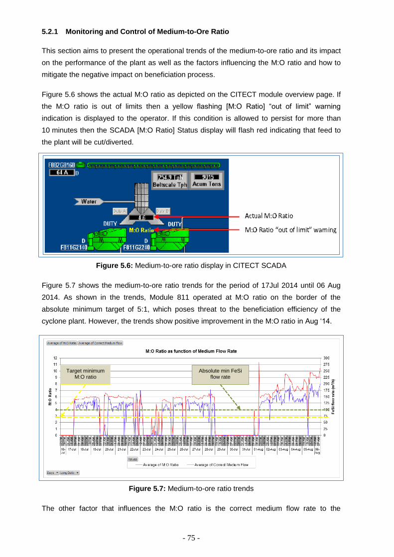
- 75 -

5.2.1 Monitoring and Control of Medium-to-Ore Ratio

This section aims to present the operational trends of the medium-to-ore ratio and its impact

on the performance of the plant as well as the factors influencing the M:O ratio and how to

mitigate the negative impact on beneficiation process.

Figure 5.6 shows the actual M:O ratio as depicted on the CITECT module overview page. If

the M:O ratio is out of limits then a yellow flashing [M:O Ratio] “out of limit” warning

indication is displayed to the operator. If this condition is allowed to persist for more than

10 minutes then the SCADA [M:O Ratio] Status display will flash red indicating that feed to

the plant will be cut/diverted.

Figure 5.6: Medium-to-ore ratio display in CITECT SCADA

Figure 5.7 shows the medium-to-ore ratio trends for the period of 17Jul 2014 until 06 Aug

2014. As shown in the trends, Module 811 operated at M:O ratio on the border of the

absolute minimum target of 5:1, which poses threat to the beneficiation efficiency of the

cyclone plant. However, the trends show positive improvement in the M:O ratio in Aug ‘14.

Figure 5.7: Medium-to-ore ratio trends

The other factor that influences the M:O ratio is the correct medium flow rate to the

Target minimum M:O ratio

Absolute min FeSi flow rate

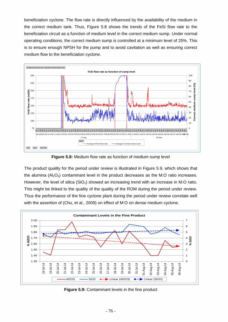
- 76 -

beneficiation cyclone. The flow rate is directly influenced by the availability of the medium in

the correct medium tank. Thus, Figure 5.8 shows the trends of the FeSi flow rate to the

beneficiation circuit as a function of medium level in the correct medium sump. Under normal

operating conditions, the correct medium sump is controlled at a minimum level of 25%. This

is to ensure enough NPSH for the pump and to avoid cavitation as well as ensuring correct

medium flow to the beneficiation cyclone.

Figure 5.8: Medium flow rate as function of medium sump level

The product quality for the period under review is illustrated in Figure 5.9, which shows that

the alumina (Al2O3) contaminant level in the product decreases as the M:O ratio increases.

However, the level of silica (SiO2) showed an increasing trend with an increase in M:O ratio.

This might be linked to the quality of the quality of the ROM during the period under review.

Thus the performance of the fine cyclone plant during the period under review correlate well

with the assertion of (Chu, et al., 2009) on effect of M:O on dense medium cyclone.

Figure 5.9: Contaminant levels in the fine product

0

1

2

3

4

5

6

7

1.30

1.40

1.50

1.60

1.70

1.80

1.90

2.00

18-J

ul-1

4

19-J

ul-1

4

20-J

ul-1

4

21-J

ul-1

4

22-J

ul-1

4

23-J

ul-1

4

24-J

ul-1

4

25-J

ul-1

4

26-J

ul-1

4

27-J

ul-1

4

28-J

ul-1

4

29-J

ul-1

4

30-J

ul-1

4

31-J

ul-1

4

01-A

ug-1

4

02-A

ug-1

4

03-A

ug-1

4

04-A

ug-1

4

05-A

ug-1

4

06-A

ug-1

4

% S

iO3

% A

l2O

3

Contaminant Levels in the Fine Product

Al2O3 SiO2 Linear (Al2O3) Linear (SiO2)

0

10

20

30

40

50

60

70

80

90

100

75

100

125

150

175

200

225

250

:06

:27

:48

:09

:30

:51

:12

:33

:54

:15

:36

:57

:18

:39

:00

:21

:41

:02

:23

:44

:05

:26

:47

:08

:29

:50

:11

:32

:53

:14

:35

:56

:17

:38

:59

:20

:41

:02

:23

:44

:05

:26

:47

:08

:29

:50

:11

:32

:53

:14

:35

:56

:17

:38

:59

:20

:41

:02

:23

:44

:05

:26

:47

:08

:29

:50

:11

:32

:53

:14

:35

:56

:17

08 AM 09 AM 10 AM 11 AM 12 PM 01 PM 02 PM 03 PM 04 PM 05 PM 06 PM 07 PM 08 PM 09 PM 10 PM 11 PM 12 AM 01 AM 02 AM 03 AM 04 AM 05 AM 06 AM 07 AM 08 AM09 AM

27-Sep 28-Sep

Co

rre

ct

me

diu

m s

um

p l

eve

l (%

)

Fe

Si fl

ow

ra

te (

m3

/h)

FeSi flow rate as function of sump level

Average of FeSi Flow rate Average of Correct Sump Level

Values

Days Hours Long Time

Average of FeSi Flow rate Average of Correct Sump Level

- 77 -

5.2.2 Monitoring and Control of Cyclone Inlet Pressure

This section aims to present the operational trends of the cyclone inlet pressure and their

impact on the performance of the plant. Figure 5.10 and Figure 5.11 illustrate the module

arrangement and feed pipeline for cyclone plant module in Sishen. The graphs depict

designs that will have an impact on the cyclone inlet pressure as well as inlet velocity.

Figure 5.10: Layout of the module feed streams

Figure 5.11: Cyclone inlet pipe arrangement

Inconsistent cyclone inlet

pipe

arrangement

Cluster 1

FeSi Medium

Distribution Tank

Correct Medium

Pump

Correct Medium

Tank

Pre-wash

Screen 1

Feed Distribution

“Hoender Spoor”

Ore & FeSi mixed on

screen discharge

chute

Cluster 2

Pre-wash

Screen 1

Ore & FeSi mixed on

screen discharge

chute

Jacko Sleeve

Manual Valve

Jacko Sleeve

Manual Valve

Feed Distribution

“Hoender Spoor”

I-3

I-4 New Flow Meter New Flow Meter

- 78 -

The purpose of the cyclone inlet feed monitoring and control is to ensure that the inlet

pressure to respective feed cyclones in cluster is constant. The cyclone inlet pressure should

remain as stable as possible under feed conditions. An ideal operating pressure ranges from

8D to 12D. The pressure differential within a cluster can undergo a 5 – 10% variation.

However, should the variation be high is an indication of system imbalances and either one

set is blocked. The inlet pressure is also been linked to the performance of the beneficiation

cyclone, where lower pressures are indicative of cyclone being prone to roping.

Pressure transmitters have been installed on each of the cyclone within a cluster. These

pressure transmitters monitor the pressure in each cyclone of a particular cluster and if there

is a difference in pressure between any of the cyclones within a cluster, then a SCADA

Cyclone Delta P “out of limit” warning will be displayed (Figure 5.12).

Figure 5.12: Cyclone and cluster monitoring display in the SCADA

Figure 5.13 shows the inlet pressure trends for the Module 811 cyclone clusters. The graph

also shows the pictorial view of the cyclone spigot operating condition for the cluster 1

cyclones taken on the 10th August 2014. This was monitored to illustrate the influence of inlet

pressure on cyclone operating condition. It can be seen that cyclone 5120 showed excellent

flaring condition and this cyclone had the highest inlet pressure indicated by pressure

transmitter PT102 trends. Similarly the 5110 cyclone that had the lowest pressure (PT101

trends) showed poorer flaring condition.

The area of concern identified for the possible inaccuracies and variation in inlet pressure of

the same cyclone cluster is the flexible feed pipe arrangement depicted in Figure 5.11. This

leads to varying flow profile to cluster’s cyclones, thereby having preferential flow for feed

pipeline with less restriction. Thus, it is imperative to have similar cyclone feed pipeline

profile to limit the impact of preferential flow as well as prevent addition pressure drops prior

slurry inlet in the cyclone.

Cyclone inlet pressure can also be influence by the medium flow balance between the two

clusters as they are fed from a common medium distribution tank. The medium flow to

clusters is control by manual “Jacko-sleeve” screw type valve on a flexible rubber spool

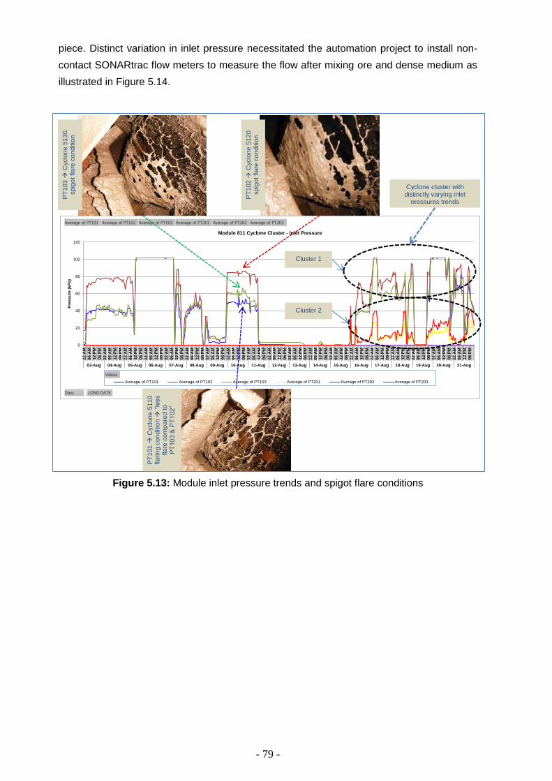
- 79 -

piece. Distinct variation in inlet pressure necessitated the automation project to install non-

contact SONARtrac flow meters to measure the flow after mixing ore and dense medium as

illustrated in Figure 5.14.

Figure 5.13: Module inlet pressure trends and spigot flare conditions

Cyclone cluster with distinctly varying inlet

pressures trends

0

20

40

60

80

100

120

12 A

M

06 A

M

12 P

M

06 P

M

12 A

M

06 A

M

12 P

M

06 P

M

12 A

M

06 A

M

12 P

M

06 P

M

12 A

M

06 A

M

12 P

M

06 P

M

12 A

M

06 A

M

12 P

M

06 P

M

12 A

M

06 A

M

12 P

M

06 P

M

12 A

M

06 A

M

12 P

M

06 P

M

12 A

M

06 A

M

12 P

M

06 P

M

12 A

M

06 A

M

12 P

M

06 P

M

12 A

M

06 A

M

12 P

M

06 P

M

12 A

M

06 A

M

12 P

M

06 P

M

12 A

M

06 A

M

12 P

M

06 P

M

12 A

M

06 A

M

12 P

M

06 P

M

12 A

M

06 A

M

12 P

M

06 P

M

12 A

M

06 A

M

12 P

M

06 P

M

12 A

M

06 A

M

12 P

M

06 P

M

12 A

M

06 A

M

12 P

M

06 P

M

12 A

M

06 A

M

12 P

M

06 P

M

12 A

M

06 A

M

12 P

M

06 P

M

03-Aug 04-Aug 05-Aug 06-Aug 07-Aug 08-Aug 09-Aug 10-Aug 11-Aug 12-Aug 13-Aug 14-Aug 15-Aug 16-Aug 17-Aug 18-Aug 19-Aug 20-Aug 21-Aug

Pre

ssu

re (

kP

a)

Module 811 Cyclone Cluster - Inlet Pressure

Average of PT101 Average of PT102 Average of PT103 Average of PT201 Average of PT202 Average of PT203

Values

Days LONG DATE

Average of PT101 Average of PT102 Average of PT103 Average of PT201 Average of PT202 Average of PT203

Cluster 1

Cluster 2

PT

102

Cyclo

ne 5

120

spig

ot fla

re c

onditio

n

PT

101

Cyclo

ne 5

110

flarin

g c

on

ditio

n

“le

ss

flare

com

pare

d t

o

PT

103 &

PT

102

”

PT

103

Cyclo

ne 5

130

spig

ot fla

re c

onditio

n

- 80 -

Figure 5.14: Cyclone cluster balance

Cyclone feed flow rate is presented in Figure 5.15. Flow rate variation greater than 15% is

regarded as having drastic impact on the system balance. (Mukherjee, et al., 2003) indicated

that higher flowrates to the cyclone would result in lower Ep, that is, high flow rates ensures

better sharpness of separation. In addition, it was found that medium stability is not affected

at high flow rates for the fine dense media. Thus, with the cyclone cluster monitoring would

ensure better control of cyclone performance thereby eliminating the effect poorer Ep in

another cluster.

Figure 5.15: Cyclone cluster feed flow rate

Cyclone cluster feed without flow rate monitor

Cyclone cluster feed with flow rate monitor

Feed distribution to individual

cyclones “Hoender Spoor”

SONARtrac flow meter for cyclone

cluster feed balance

“Jacko-Sleeve” Valves

6015768

Stamp

- 81 -

5.2.3 Monitoring and Control of Density Differential Measurement

Figure 5.16 illustrates the density trends of the feed medium and the cyclone overflow and

underflow medium during the commissioning of the DMCT110 unit. The trends present data

after quick calibration of the units using one point measure in order to validate the operability

of the instrument from default values. Apart from optimisation and full calibration, the trends

show that the system is functioning properly with the values of the underflow stream being

higher than the feed and ditto for value of overflow stream being lower than the feed density.

Figure 5.16: FeSi Medium density trends

Figure 5.17 illustrates the density differential trends determined from online measurement

during commissioning and quick calibration phase. The density differential tends show some

very positive and encouraging results that are worth a mention. It can be seen that point A in

the graph during the period of 30th Sept is indicative of medium instability with the overflow

and underflow densities diverging from each other while the feed medium density remained

relatively constant. This can be attributed to dense medium segregation in the cyclone,

where the overflow stream comprises of finer size fraction. In addition, the trends show

steady state operations during period 5th Oct 2014 until 7th Oct 2014 as indicated by point B

where the underflow and overflow densities are trending relative to the feed control density.

The manual density differential measurements are shown in Figure 5.18. The trends

illustrates that the density differential is within the allowable metallurgical best practice.

However, the online trends showed a slightly high differential which might be attributed to

medium instability.

2.80

2.90

3.00

3.10

3.20

3.30

3.40

3.50

3.60

3.70

3.80

04:3

4:24

PM

06:0

8:08

PM

07:4

1:52

PM

09:1

5:36

PM

10:4

9:20

PM

12:2

3:04

AM

01:5

6:48

AM

03:3

0:32

AM

05:0

4:16

AM

06:3

7:59

AM

08:1

1:43

AM

09:4

5:27

AM

11:1

9:11

AM

12:5

2:55

PM

02:2

6:39

PM

04:0

0:23

PM

05:3

4:07

PM

07:0

7:51

PM

08:4

1:35

PM

10:1

5:19

PM

11:4

9:03

PM

01:2

2:47

AM

02:5

6:30

AM

04:3

0:14

AM

06:0

3:58

AM

07:3

7:42

AM

09:1

1:26

AM

10:4

5:10

AM

12:1

8:54

PM

01:5

2:38

PM

03:2

6:22

PM

05:0

0:06

PM

06:3

3:50

PM

08:0

7:34

PM

09:4

1:17

PM

11:1

5:01

PM

12:4

8:45

AM

02:2

2:29

AM

03:5

6:13

AM

05:2

9:57

AM

07:0

3:41

AM

08:3

7:25

AM

Average of Feed Medium Average of DT101 Average of DT103 Average of DT102 Average of DT104

Values

Long Date

Average of Feed Medium Average of DT101 Average of DT103 Average of DT102 Average of DT104

Calibration & PLC linkage via Profibus

Re-linking unit to PLC using I/O Comms cable.

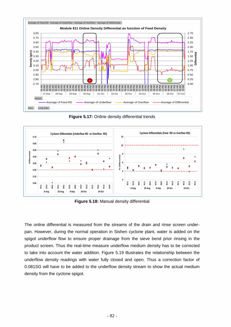
- 82 -

Figure 5.17: Online density differential trends

Figure 5.18: Manual density differential

The online differential is measured from the streams of the drain and rinse screen under-

pan. However, during the normal operation in Sishen cyclone plant, water is added on the

spigot underflow flow to ensure proper drainage from the sieve bend prior rinsing in the

product screen. Thus the real-time measure underflow medium density has to be corrected

to take into account the water addition. Figure 5.19 illustrates the relationship between the

underflow density readings with water fully closed and open. Thus a correction factor of

0.081SG will have to be added to the underflow density stream to show the actual medium

density from the cyclone spigot.

0.00

0.25

0.50

0.75

1.00

1.25

1.50

1.75

2.00

2.25

2.50

2.75

2.70

2.80

2.90

3.00

3.10

3.20

3.30

3.40

3.50

3.60

3.70

3.80

05 A

M

10 A

M

03 P

M

08 P

M

01 A

M

06 A

M

11 A

M

04 P

M

09 P

M

02 A

M

07 A

M

12 P

M

05 P

M

10 P

M

03 A

M

08 A

M

01 P

M

06 P

M

11 P

M

04 A

M

09 A

M

02 P

M

07 P

M

12 A

M

05 A

M

10 A

M

03 P

M

08 P

M

01 A

M

06 A

M

11 A

M

04 P

M

09 P

M

02 A

M

07 A

M

12 P

M

05 P

M

10 P

M

03 A

M

08 A

M

01 P

M

06 P

M

11 P

M

04 A

M

09 A

M

02 P

M

07 P

M

12 A

M

05 A

M

10 A

M

27-Sep 28-Sep 29-Sep 30-Sep 01-Oct 02-Oct 03-Oct 04-Oct 05-Oct 06-Oct 07-Oct

Dif

fere

nti

al

De

ns

ity (

g/c

c)

Module 811 Online Density Differential as function of Feed Density

Average of Feed RD Average of Underflow Average of Overflow Average of Differential

Values

Days Long Date

Average of Feed RD Average of Underflow Average of Overflow Average of Differential

A B

0.00

0.10

0.20

0.30

0.40

0.50

0.60

0.70

81

1

81

3

80

1

81

1

80

1

81

2

80

2

81

2

81

3

81

1

81

2

81

3

814

6-Aug 25-Aug 9-Sep 20-Oct 24-Oct

Dif

fere

nti

al

Cyclone Differentials (Underflow RD vs Overflow RD)

0

3

6

9

12

15

81

1

81

3

80

1

81

1

80

1

81

2

80

2

81

2

81

3

81

1

81

2

813

81

4

6-Aug 25-Aug 9-Sep 20-Oct 24-Oct

% D

iffe

re

nti

al

Cyclone Differentilals (Feed RD vs Overflow RD)

- 83 -

Figure 5.19: Relationship of the underflow medium density with and without water dilution

- 84 -

CHAPTER 6: MODELLING OF DENSE MEDIUM CYCLONE CIRCUIT

6 DENSE MEDIUM CYCLONE MODELLING INTRODUCTION

A Simulink program was utilised to simulate the performance of the cyclone module based

on the existing models from literature such as the well-known Wood’s empirical model

described in section 2.2.4. This was also complemented by use of equations derived by

(Meyer, 2010) to model the dense medium circuit and supplementary unit processes is

derived from the principle of conservation that is obeyed by all physical systems as cited by

(Stephanopoulos, 1984). Thus, the principle of conservation for mass into a system can be

summarised as follows:

…Equation 6.1

The above conservation of mass principle described in Equation 6.1 was used by (Meyer,

2010) to develop mathematical models for the dense medium cyclone and heavy medium

make-up tank. With the development of this process models, it was assumed that the rates

of change for the mass splits to the cyclone overflow and underflow is proportional to the

dense medium densities in cyclone underflow and overflow. Thus, equation 6.2 to 6.4 was

derived while assuming the steady state volumetric flows, that is, 𝑄𝑖𝑛𝑙𝑒𝑡 = 𝑄𝑜/𝑓 + 𝑄𝑢/𝑓.

Vc,odρc,o

dt+ Vc,u

dρc,u

dt= Wc,i − Qc,oρc,o − Qc,uρc,u … Equation 6.2

By assuming that the rate of change in mass to the overflow and underflow to be

proportional to the medium density differential in underflow and overflow stream, (Meyer,

2010), deducted that the conservation of mass would results in the following relationship:

Vc,odρc,o

dt= Kc,o(ρc,i − ρc,o) ∙ waste … Equation 6.3

Vc,udρc,u

dt= Kc,u(ρc,i − ρc,u) ∙ product … Equation 6.4

While the above mentioned models are relatively easy to follow and contains all of the

components that provide sensitivity to changes in operation, i.e. ore feed rates, cyclone inlet

density, cyclone size, particle sizes, FeSi size etc. However, these models come with the

disclaimer that it is relevant to a specific cyclone setup and operating conditions. Both

(Wang, 2009) and (Petersen, 2010) conceded that this takes the model out of the hands of

anyone who wants to use it independently in an applied fashion. Thus in order for the user to

apply this in their operational environment, the model has to be “re-engineered” for their own

conditions, particularly determining constants and other fitting parameters.

𝐴𝑐𝑐𝑢𝑚𝑢𝑙𝑎𝑡𝑖𝑜𝑛 𝑜𝑓 𝑀

𝑡𝑖𝑚𝑒 𝑝𝑒𝑟𝑖𝑜𝑑=

𝐼𝑛𝑙𝑒𝑡 𝐹𝑙𝑜𝑤 𝑜𝑓 𝑀

𝑡𝑖𝑚𝑒 𝑝𝑒𝑟𝑖𝑜𝑑−

𝑂𝑢𝑡𝑙𝑒𝑡 𝐹𝑙𝑜𝑤 𝑜𝑓 𝑀

𝑡𝑖𝑚𝑒 𝑝𝑒𝑟𝑖𝑜𝑑+

𝑀 𝑔𝑒𝑛𝑒𝑟𝑎𝑡𝑒𝑑

𝑡𝑖𝑚𝑒 𝑝𝑒𝑟𝑖𝑜𝑑−

𝑀 𝑐𝑜𝑛𝑠𝑢𝑚𝑒𝑑

𝑡𝑖𝑚𝑒 𝑝𝑒𝑟𝑖𝑜𝑑

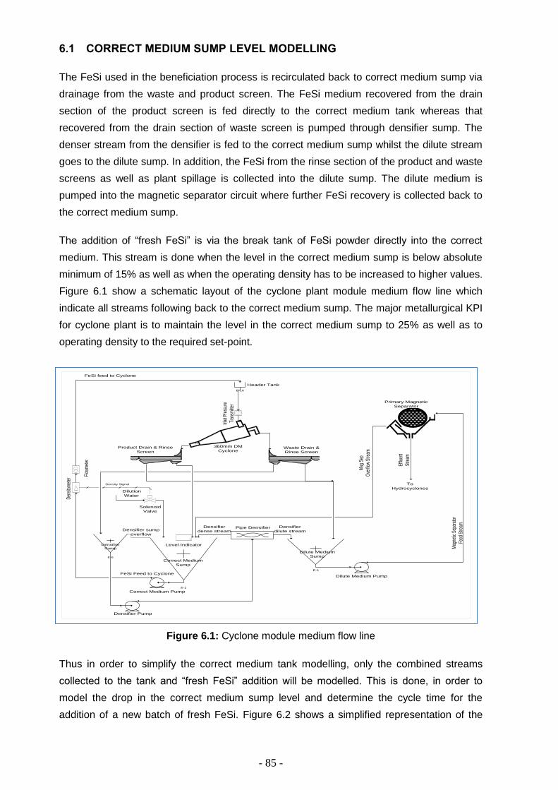
- 85 -

6.1 CORRECT MEDIUM SUMP LEVEL MODELLING

The FeSi used in the beneficiation process is recirculated back to correct medium sump via

drainage from the waste and product screen. The FeSi medium recovered from the drain

section of the product screen is fed directly to the correct medium tank whereas that

recovered from the drain section of waste screen is pumped through densifier sump. The

denser stream from the densifier is fed to the correct medium sump whilst the dilute stream

goes to the dilute sump. In addition, the FeSi from the rinse section of the product and waste

screens as well as plant spillage is collected into the dilute sump. The dilute medium is

pumped into the magnetic separator circuit where further FeSi recovery is collected back to

the correct medium sump.

The addition of “fresh FeSi” is via the break tank of FeSi powder directly into the correct

medium. This stream is done when the level in the correct medium sump is below absolute

minimum of 15% as well as when the operating density has to be increased to higher values.

Figure 6.1 show a schematic layout of the cyclone plant module medium flow line which

indicate all streams following back to the correct medium sump. The major metallurgical KPI

for cyclone plant is to maintain the level in the correct medium sump to 25% as well as to

operating density to the required set-point.

Figure 6.1: Cyclone module medium flow line

Thus in order to simplify the correct medium tank modelling, only the combined streams

collected to the tank and “fresh FeSi” addition will be modelled. This is done, in order to

model the drop in the correct medium sump level and determine the cycle time for the

addition of a new batch of fresh FeSi. Figure 6.2 shows a simplified representation of the

E-2

Correct Medium Pump

E-5

E-6

Densifier Pump

Dilute Medium Pump

E-10

P-15

Primary Magnetic

Separator

360mm DM

CycloneWaste Drain &

Rinse Screen

Product Drain & Rinse

Screen

Header Tank

Correct Medium

Sump

Dilute Medium

Sump

Densifier

Sump

FeSi Feed to Cyclone

FeSi feed to Cyclone

Dilution

Water

Solenoid

Valve

Density Signal

L

Level Indicator

To

Hydrocyclones

Efflu

ent

Stre

am

Mag

netic

Sep

arat

or

Feed

Stre

am

Den

sito

met

er

Flow

met

er

Densifier sump

overflow

Mag

Sep

Ove

rflow

Stre

am

Inle

t Pre

ssur

e

Tran

smitt

er

Densifier

dilute streamPipe DensifierDensifier

dense stream

- 86 -

correct medium tank system utilised for modelling purposes. The current medium tank

design is a truncated conical tank. Thus, the equations 2.11 to 2.13 as described in section

2.2.3 are applicable for determining the capacity of the correct medium tank for a cyclone

module.

The dimensions of the correct medium tank are as follows:

Bottom diameter = 610 mm

Total tank height = 2,264 mm

Top part diameter = 3,500 mm

To simplify the modelling of the tank height in order to determine when manual “fresh FeSi

addition” must happen, it was assumed that the effective area of the medium tank does not

change with change in medium height in the tank. Thus, the modelling of rate of change of

medium level in the tank can be simulated utilising the conservation of mass taking into

account the rate of medium flow in and out of the tank as follows:

𝐴𝑡𝑑ℎ𝑡

𝑑𝑟= 𝑄𝑡,𝑚𝑒𝑑 + 𝑄𝑡,𝑑𝑖𝑠 − 𝑄𝑡 … Equation 6.5

Figure 6.2: Simplified representation of correct medium tank

Figure 6.3 illustrates the internal structure of the Simulink for the modelling of correct

medium tank level. The structure shows flow rate of medium recovered back into the circuit

by utilising the random flow rate generator, with the average flow of 155 m3/h, in order to

mimic the plant operating conditions. The parameter selection was selected to denote a

mean of 155 representing the average design flow rate for the plant whilst the variance was

kept a default value of 1. The out flow stream denotes medium fed to the beneficiation

circuit which is inclusive of the FeSi lost via adhesion losses as well as effluent stream of the

magnetic separator. A signal builder is incorporated to mimic the disturbance attributed to

the addition of the “fresh FeSi powder” via current manual bag breaker system.

Correct Medium

Tank

Correct medium

pump

Fresh FeSi addition

(Make-up medium disturbance)FeSi recovered from the circuit

Qt, dis

t,dis

Wt, med

Qt, med

t, med

Qt

t

Correct medium

feed to

beneficiation

circuit

Vt

ht

At

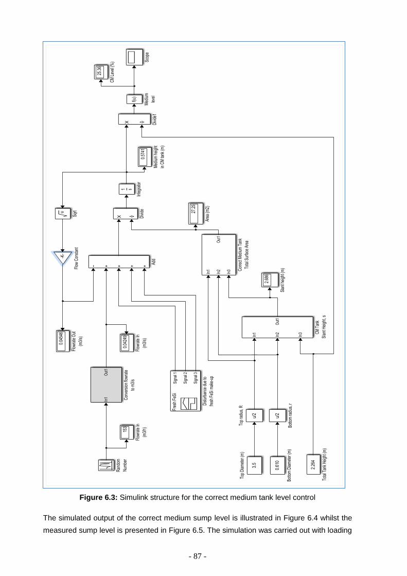
- 87 -

Figure 6.3: Simulink structure for the correct medium tank level control

The simulated output of the correct medium sump level is illustrated in Figure 6.4 whilst the

measured sump level is presented in Figure 6.5. The simulation was carried out with loading

- 88 -

a disturbance mimicking the manual addition of “fresh FeSi” powder in the correct medium

sump. Point A in Figure 6.5 indicate the period when the module was shut-down which

shows an increase in the sump level due to the FeSi medium in the circuit gravitating back to

the correct medium sump.

The correct medium sump level control can easily be controlled by proper conventional PID

controller. This will ensure that the level control is maintained at a set-point value and able to

accept and/or adapt to process disturbances. This can be achieved by automating the “fresh

FeSi make-up system. However, the current manual fresh FeSi addition method

necessitated that the modelling be done to mimic such disturbance. Thus, the current model

set-up will suffices for the indication of when and the frequency of the manual of the “fresh

FeSi batch” in the system.

For the system with automated fresh FeSi make-up system, the design of the controller will

be similar to that described by (Aslam & Haider, 2011) and (Meyer, 2010). The design model

will consist of the controller that will maintain the dense medium level in the sump to a

desired set-point as well as at the required operating density while rejecting the disturbance

introduced by make-up FeSi and recovered FeSi streams.

Figure 6.4: Simulated response of the correct medium sump level

- 89 -

Figure 6.5: Plant measured correct medium sump level

6.2 CYCLONE PERFORMANCE MODELLING

A dense medium cyclone model has been developed for the Sishen iron ore DMS plant, with

a specific focus on underflow and overflow medium density, which incorporated the current

state of the art model by Woods that relies heavily on calibration constants. The model also

incorporates the medium flow split in the cyclone. In view of the difficulty in applying the

Woods model, a model structure that has few calibration constants and specifically uses

operational state variables has been designed.

The modelling of the cyclone Module 811 is based on the following baseline setup

conditions:

Cyclone diameter (Dc) : 360 mm

Cone angle : 10 degrees

Spigot diameter (Du) : 100 mm

Vortex diameter (Do) : 125 mm

Barrel length : 200 mm

Cone length : 535 mm

Design operational parameters are:

Ore feed rate = 180 t/h (average)

Ore particle density = 4.50 t/m3

Medium flow rate = 150 m3/h (absolute min)

Medium operating density = 3.4 t/m3

Viscosity = 0.02 Pa.s

The Simulink structure to model the performance of the dense medium cyclones based on

the total conservation of mass principle and incorporation of the Wood’s sub-models is

0

10

20

30

40

50

60

70

80

90

100

08 A

M

09 A

M

10 A

M

11 A

M

12 P

M

01 P

M

02 P

M

03 P

M

04 P

M

05 P

M

06 P

M

07 P

M

08 P

M

09 P

M

10 P

M

11 P

M

12 A

M

01 A

M

02 A

M

03 A

M

04 A

M

05 A

M

06 A

M

07 A

M

08 A

M

09 A

M

27-Sep 28-Sep

Leve

l (%

)Correct Medium Sump Level

Days Long Time

Average of Correct Sump Level

A

- 90 -

presented in Figure 6.6. A random number generator was incorporated in the model to mimic

the variation if the ore feed rate (t/h) in the cyclone module. The parameter selection was

kept at a mean of 180 to denotes the average feed design feed rate whilst the variance was

kept at default value of 1. This was done to simulate the actual plant performance around the

set-point throughput of 180t/h.

The structure is used to simulate the cyclone underflow and overflow densities. Detailed sub-

systems for the Simulink internal structure for modelling the cyclone module’s overflow and

underflow densities as well as the percentage of medium split to overflow stream are

presented in Figure 6.7 and Figure 6.8. A function block to describe the medium behaviour

was incorporated in sub-system depicted in Figure 6.7 as adopted from the Wood’s sub-

model 4, which aim to determine the medium density of the overflow stream as

described in equation 2.10 (Section 2.2.4).

Figure 6.6: Internal structure of the Simulink model for the modelling of the cyclone

underflow and overflow density

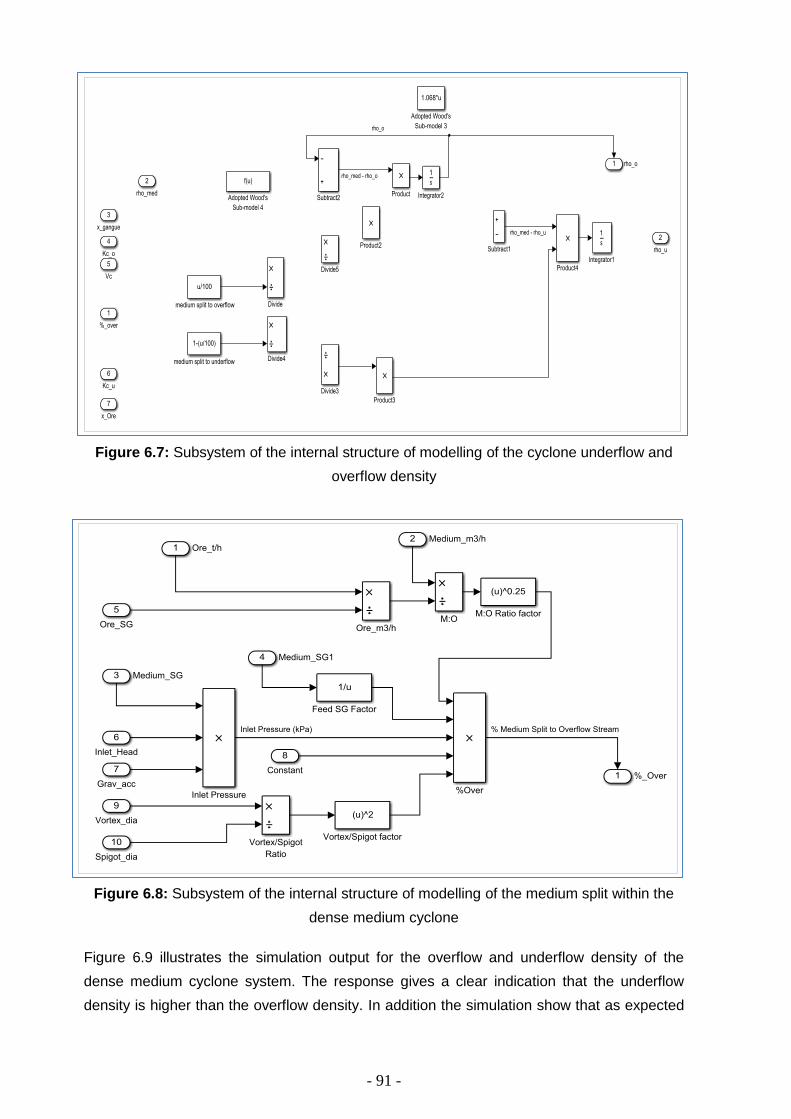
- 91 -

Figure 6.7: Subsystem of the internal structure of modelling of the cyclone underflow and

overflow density

Figure 6.8: Subsystem of the internal structure of modelling of the medium split within the

dense medium cyclone

Figure 6.9 illustrates the simulation output for the overflow and underflow density of the

dense medium cyclone system. The response gives a clear indication that the underflow

density is higher than the overflow density. In addition the simulation show that as expected

- 92 -

the values of the underflow stream is higher that the feed density whilst the overflow stream

being lower than feed density.

The model output is the medium density in the spigot, which is underflow density. This can

be correlated to the cyclone cut-point density, however, has no explicit reference to

sharpness of separation. The model structure has been tested for the sake of diagnosing if

the model has all of the salient features that would be required to adequately mimic DMS

cyclone operation and the separation of a range of particle densimetric profile. Results show

that the model is highly educational, providing specific details as to the reason why

separation dynamics would change for any change in operating parameters.

The model output correlate well with the plant measured data under stable condition as

depicted in Point B of Figure 5.17, while the plant was operated at feed density of 3.40 SG.

Thus this outcome indicates that the model predicts the cyclone underflow and overflow

density accurately. The simulated output indicated a density differential of 0.304 SG whilst

the plant real-time measurement showed density differential ranging between 0.484 and

1.476 SG (average ~ 0.801SG).

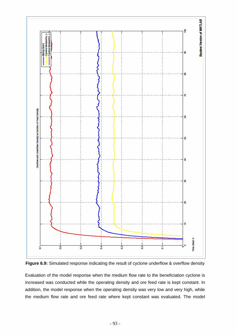
- 93 -

Figure 6.9: Simulated response indicating the result of cyclone underflow & overflow density

Evaluation of the model response when the medium flow rate to the beneficiation cyclone is

increased was conducted while the operating density and ore feed rate is kept constant. In

addition, the model response when the operating density was very low and very high, while

the medium flow rate and ore feed rate where kept constant was evaluated. The model

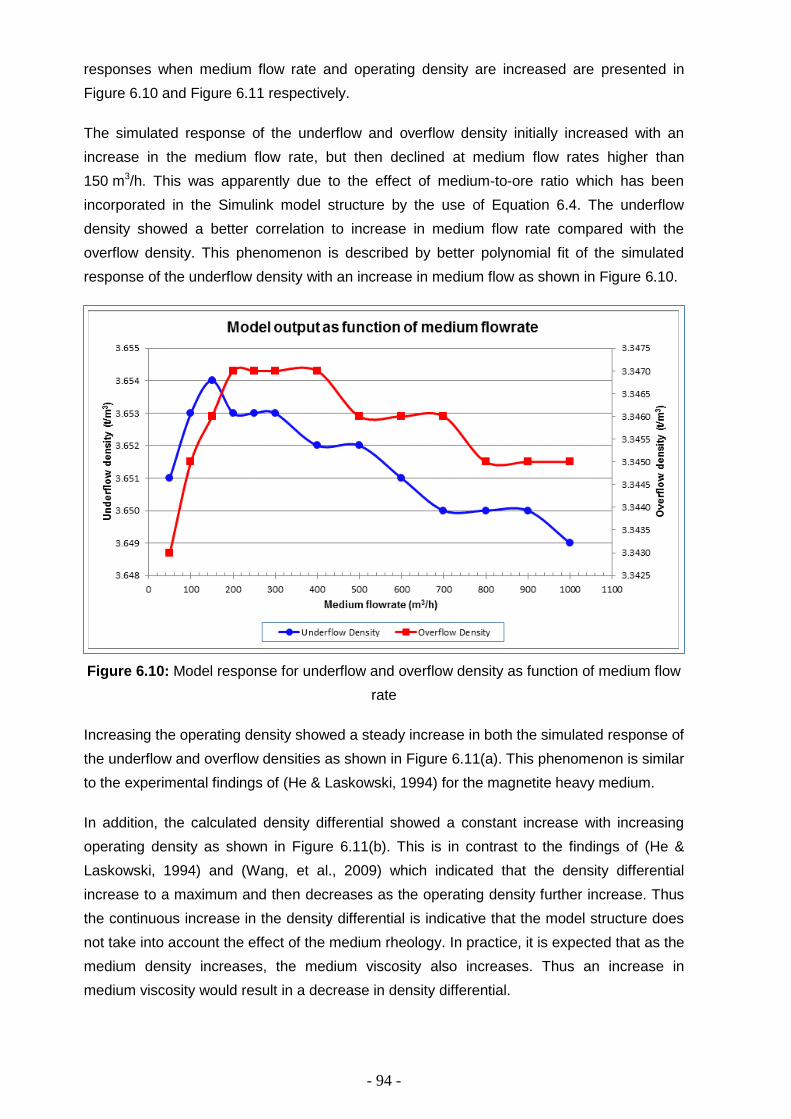
- 94 -

responses when medium flow rate and operating density are increased are presented in

Figure 6.10 and Figure 6.11 respectively.

The simulated response of the underflow and overflow density initially increased with an

increase in the medium flow rate, but then declined at medium flow rates higher than

150 m3/h. This was apparently due to the effect of medium-to-ore ratio which has been

incorporated in the Simulink model structure by the use of Equation 6.4. The underflow

density showed a better correlation to increase in medium flow rate compared with the

overflow density. This phenomenon is described by better polynomial fit of the simulated

response of the underflow density with an increase in medium flow as shown in Figure 6.10.

Figure 6.10: Model response for underflow and overflow density as function of medium flow

rate

Increasing the operating density showed a steady increase in both the simulated response of

the underflow and overflow densities as shown in Figure 6.11(a). This phenomenon is similar

to the experimental findings of (He & Laskowski, 1994) for the magnetite heavy medium.

In addition, the calculated density differential showed a constant increase with increasing

operating density as shown in Figure 6.11(b). This is in contrast to the findings of (He &

Laskowski, 1994) and (Wang, et al., 2009) which indicated that the density differential

increase to a maximum and then decreases as the operating density further increase. Thus

the continuous increase in the density differential is indicative that the model structure does

not take into account the effect of the medium rheology. In practice, it is expected that as the

medium density increases, the medium viscosity also increases. Thus an increase in

medium viscosity would result in a decrease in density differential.

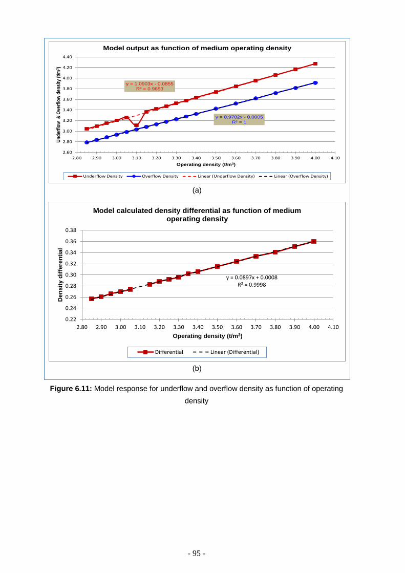
- 95 -

Figure 6.11: Model response for underflow and overflow density as function of operating

density

y = 1.0903x - 0.0855R² = 0.9853

y = 0.9782x - 0.0005R² = 1

2.60

2.80

3.00

3.20

3.40

3.60

3.80

4.00

4.20

4.40

2.80 2.90 3.00 3.10 3.20 3.30 3.40 3.50 3.60 3.70 3.80 3.90 4.00 4.10

Un

der

flo

w &

Ov

erfl

ow

den

sity

(t/

m3 )

Operating density (t/m3)

Model output as function of medium operating density

Underflow Density Overflow Density Linear (Underflow Density) Linear (Overflow Density)

y = 0.0897x + 0.0008R² = 0.9998

0.22

0.24

0.26

0.28

0.30

0.32

0.34

0.36

0.38

2.80 2.90 3.00 3.10 3.20 3.30 3.40 3.50 3.60 3.70 3.80 3.90 4.00 4.10

Den

sit

y d

iffe

ren

tial

Operating density (t/m3)

Model calculated density differential as function of medium operating density

Differential Linear (Differential)

(a)

(b)

- 96 -

CHAPTER 7: CONCLUSIONS AND RECOMMENDATIONS

7 CONCLUSIONS AND RECOMMENDATIONS

7.1 CONCLUSIONS

7.1.1 Ore and FeSi Characterisation Conclusions

Ore characterisation is mainly focused on understanding the densimetric profile of the ore

body, in order to determine the probability to produce a saleable product as well as

predicting the expected yields and quality. This is done to utilise the endowment entrusted

upon the operating entity by the government and shareholders to treat the mineral resource

to its full potential. Understanding of the beneficiation potential of the ore body will assist the

mine planning and processing plant to optimise the product tons and quality. This will ensure

proper marketing plans that are synchronised to beneficiation plant due whose performance

will depend on mining block reserves. Certain mining blocks have potential to produce

varying product grades with different recoveries.

Ore characterisation was conducted on the GR80 mining block, low-grade stockpiles (i.e. C-

grade ore reserves & Jig discard and dense medium separation (DMS) run-of-mine (ROM)

material. The GR80 material was characterised as having low proportion of near-density

material and will be easy to beneficiate as well as producing high volumes of high grade

product. Furthermore, it was revealed that the 2014 DMS ROM had an increased proportion

of low-density material; however this material was also had low proportion of near-density

material.

The low-grade stockpiles was characterised by high proportion of near density material,

which necessitate the beneficiation process to operate at high density in excess of 3.8 t/m3.

Thus with higher operating density, the dense medium might lead to viscosity problems

which have to be managed and controlled efficiently. Therefore, characterisation of the FeSi

medium was imperative to understand its behaviour and potential influence to beneficiation

of low-grade stockpiles and mining blocks with elevated proportion of near-density material.

As the proportion of near-density waste material increases in the run-of-mine (ROM), it is

necessary to beneficiate the material at elevated operating medium densities. However,

when cyclones are operated at high densities, the negative influences of the medium

viscosity become more apparent and thus influence the separation efficiency.

Heavy medium, ferrosilicon (FeSi) characterisation looked at identifying the effects of

viscosity on the FeSi stability and whether there is a need for viscosity modifier should the

need arise. Thus, the importance of controlling the stability, viscosity, and density of the

medium must not be under-estimated and can very often override the improvements

attainable through better designs of cyclones. Furthermore, the slurry mixture of the heavy

medium utilised for the purpose of dense medium separation should be non-detrimental to

- 97 -

the effectiveness of separation in the DMS Fine cyclone plant. Medium characterisation

showed that removal of ultra-fines leads to unstable media as indicated by faster settling

rates. This would result in medium segregation in the beneficiation cyclone thereby leading

to unacceptable high density differential which will negatively impact the cut-point shift and

cause high yield losses to waste.

FeSi characterisation looked at various ways of reducing the viscosity of ferrosilicon (FeSi).

Coarse and Process FeSi were tested with a portion of fines removed and a viscosity

modifier was tested to see how this affects the FeSi flow behaviour. The viscosity modifier

used for this test work was DP 725.

The heavy medium stability characteristics were determined through the static and vertical

pipe settling tests. The bench top settling tests show that the coarse FeSi with viscosity

modifier settles out the fastest whilst the coarse FeSi less fines settles faster than the coarse

FeSi without fines removed. Thus, this proves that the content of ultra-fines proportion in the

heavy medium improves the medium stability.

Contrary to the bench top settling test, the pipe loop settling tests showed that the coarse

FeSi with viscosity modifier was significantly more stable compared to the other slurries

tested. The vertical tube viscometer tests proved that removing the fines made no significant

difference to the rheology of the coarse FeSi or the process FeSi. The viscosity modifier

reduced the viscosity of the coarse FeSi and dispersed the particles in the slurry thus

keeping them in suspension longer than otherwise possible.

7.1.2 Automation and Modelling Conclusions

The overall control of the metallurgical processes is Sishen’s Cyclone Plant is still done on

manual basis and thus operation still varies from person-to-person and/or from shift-to-shift.

This result in some of the process data and trends not being available online as well as

being captured inaccurately. Furthermore, this negatively affects the traceability and

reproducibility of the production metallurgical key performance indicators (KPI’s) as well as

process stability and efficiency. However, clear understanding of key operational parameters

and being able to figure them out, allows process controllers and metallurgists to implement

the control philosophy for the advanced process control.

It has been demonstrated that real-time online measurements are crucial to maintain

processing plant stability and efficiency thereby ensuring that the final product grade and its

value is not eroded. In addition, online measurement provides feedback to process operators

and managers, to allow full control of the process as well as improving reaction time to

changes such as variations in the quality of feed ore body. This, in turn, prevents and/or

minimizes value losses and improves the economics of the process by controlling finished

product specification and optimization of the operating cost.

- 98 -

Modelling and automated control is aimed at maintaining process stability, improving plant

throughput as well as processing efficiency. The fundamental mathematical modelling

technique is capable of providing detailed information about the dense medium dynamics

within the cyclone. In addition, Simulink modelling by incorporating the popular industry

Woods’ empirical model allows for a better understanding of the performance of dense

medium cyclone and can be utilised as a trouble-shooting tool.

Modelling and automation of the key metallurgical parameters for the cyclone plant circuit

was achieved by installation of appropriate instrumentation and interlocking to the

programmable logic control (PLC). This allowed for the control of the correct medium sump

level, cyclone inlet pressure, medium-to-ore ratio as well as online monitoring of density

differential as “proxy” for medium rheological characteristics.

The benefit of modelling and simulation allows the virtual investigation and optimisation of

the processing plant behaviour as well as analysis of the impact of varying ore

characteristics, throughput variations and changing operating parameters. Linking models to

automated plant instrumentation would be able to warn abnormal process behaviour as well

as identifying bottlenecks. In addition, Modelling and steady-state simulation can be utilised

for the prediction of the metallurgical plant efficiency where automated and real-time online

measurements cannot be obtained.

7.2 RECOMMENDATIONS FOR FUTURE WORK

Currently the system is only monitoring and trending data, thus activation of the control and

interlocking described in this document should be been activated with the roll-out phase of

the automation of the entire cyclone plant module.

Kumba Iron Ore is in the process of improving processing stability by the deployment of

advanced process control at the DMS plant. Thus, the advanced process control systems

can utilise MatLAB Simulink built-in mathematical models as central element in the

controllers’ calculations for “Model Predictive Control”.

Construction of the operational performance monitoring reports will be valuable as these

reports will focus on any constraints that can negatively influence process performance as

well as highlighting processing opportunities. Furthermore, these reports will assist in

keeping track of the processing plant state and also be usable for optimisation work.

- 99 -

REFERENCES AND APPENDICES

REFERENCES

Abu-Khalaf, M., Chen, R. & Turevskiy, A., 2010. MathWorks. [Online] Available at:

http://www.mathworks.com/company/newsletters/articles/pid-control-design-made-easy.html

Accessed 23 April 2014].

Anon., n.d. Principles: Dense Medium Cyclones. [Online] Available at:

http://www.portaclone.co.za/pr_cyclo.htm Accessed 10 Jan 2014].

Aravind, P., Valluvan, M. & Saranya, M., 2013. Simulation based modeling and

implementation of adaptive control technique for non linear process tank. International

Journal of Computer Applications, Vol. 68(No. 16), pp. pp.1-5.

Aslam, F. & Haider, M. Z., 2011. An implementation and comparative analysis of PID

controller and their auto tuning method for three tank liquid level control. International

Journal of Computer Applications, Vol. 21(No. 8), pp. pp.42-45.

Atkinson, B. et al., 2012. Dense Medium Cyclone Handbook. s.l.:HMC Processing, ACARP.

Bekker, E., 2012. Cyclone Design and Application. Johannesburg: Multotec and

Witwatersrand University.

Bekker, E., 2012. Cyclone Design and Application. Johannesburg: Multotec and

Witwatersrand University.

Björn, A. et al., 2012. Rheological Characterization, Sweden: InTech.

Chu, K. W., Wang, B., Yu, A. B. & Vince, A., 2009. CFD-DEM modelling of multiphase flow

in dense medium cyclone. Powder Technology, Volume 193, pp. 235-247.

de Villiers, R., Muller, D. & van Rooyen, J., 2014. Presentation: Intergrated Control Strategy

for Regulatory, Advanced and Optimisation Control for Mine, Plant and Logistics. s.l.:Anglo

American.

Doll, A., 2014. http://www.codecogs.com/d-ox/engineering/materials/rosin_rammler.php.

[Online] Available at: https://www.sagmilling.com/articles/2/view/?s=1 Accessed 20

September 2014].

Gochin, R. J. & Smith, M. R., 1983. Dense Medium Separation. Part 1: An introduction to the

theory and practice. Mining Magazine, December, pp. pp. 453-460.

Gupta, A. & Yan, D. S., 2006. Mineral Processing Design and Operations: An Introduction.

Oxford, UK: Elsevier.

He, Y. B. & Laskowski, J. S., 1994. Effect of dense medium properties on the separation

performance of a dense medium cyclone. Minerals Engineering, Vol. 7(Nos 2/3), pp. pp.

209-221.

- 100 -

King, R. P., 2001. Modeling and Simulation of Mineral Processing Systems. Linacre House,

Jordan Hill, Oxford: Butterworth-Heinemann.

Magwai, M. K. & Bosman, J., 2008. The effect of cyclone geometry and operating conditions

on spigot capacity of dense medium cyclones. International Journal of Mineral Processing,

Volume Vol. 86, pp. pp. 94-103.

Meyer, E. J., 2010. The development of dynamic models for a dense medium separation

circuit in coal beneficiation. Pretoria: Faculty of Engineering, the Built Environment and

Information Technology. University of Pretoria.

Mukherjee, A. K., Sripriya, R., Rao, P. V. & Das, P., 2003. Effect of increase in feed inlet

pressure on feed rate of dense media cyclone. International Journal of Mineral Processing,

Volume Vol. 69, pp. pp. 259-274.

Myburgh, H. A., 2006. The influence of the quality of ferrosilicon on the rheology of dense

medium and the ability to reach higher densites. s.l., The Journal of the Southern African

Institute of Mining and Metallurgy.

Nabbie, A., 2012. Owner's manual for the Dense Medium Controller. Rev: 1.4 ed. s.l.:De

Beers Group Services.

Napier-Munn, T. J., Dunglison, M. & Shi, F., 1994. The rheological properties and selection

of ferrosilicon dense media. South Africa, Samancor.

Narasimha, M., Brennan, M. S. & Holtham, P. N., 2006. Numerical simulation of magnetite

segregation in a dense medium cyclone. Minerals Engineering, Volume 19, pp. 1034 - 1047.

Petersen, K. R., 2010. Understanding inlet pressure in cyclone operation and process

design. s.l., The Southern African Institute of Mining and Metallurgy, pp. pp. 233-240.

Saad, M., Albagul, A. & Abueejela, Y., 2013. Performance comparison between PI and

MRAC for coupled-tank system. Journal of Automation and Control Engineering, Vol. 2(No.

3), pp. pp 316-321.

Shyan, C. W., Padmesh, T. V. N. & Suresh Manic, K., 2013. Controller tuning for a nonlinear

liquid level system. EURECA, pp. pp 17 - 18.

Sripriya, R. et al., 2001. Critical evaluation of factors affecting the operation of dense

medium cyclones treating medium coking coals. International Journal of Mineral Processing,

Volume Vol. 63, pp. pp. 191 - 206.

SRK Consulting Engineers, 2006. CPR on the material properties which will be incorporated

into Exxaro and Kumba Iron Ore, s.l.: Kumba Resources Limited.

Stephanopoulos, G., 1984. Chemical Process Control: An introduction to theory and

practice. Englewood Cliffs, New Jersey 07632: Prentice-Hall International, Inc.

- 101 -

Tom, P., 2014. Control Philosophy for the automated control and monitoring of dense media

circuit for cyclone plant, s.l.: Anglo American Kumba Iron Ore.

van Sittert, F. & Malloch, R., n.d. Proposal for FeSi rheology test for Kumba Iron Ore.

s.l.:Paterson and Cooke.

Wang, B., 2009. PhD Thesis: Modelling the multiphase flow in cyclones, s.l.: The University

of New South Wales.

Wang, B., Chu, K. W., Yu, A. B. & Vince, A., 2009. Numerical studies of the effects of

medium properties in dense medium cyclone operations. Minerals Engineering, Volume Vol.

22, pp. pp. 931-943.

Wills, B. A. & Napier-Munn, T. J., 2006. Wills' Mineral Processing Technology: An

Introduction to the Practical Aspects of Ore Treatment and Mineral. 7th ed. s.l.:Elsevier

Science & Technology Books.

- 102 -

APPENDICES

APPENDIX A: ORE CHARACTERISATION

7.2.1 Appendix A.1 – Material Type Classification

Kl

201 202 203 501

301 302 303 601

CLAS

S

stock

pile

101Bruce

A

102Bruce

A

201 BIF

202 BIF

203 C

401SP

H4

402SP

EKG

301SP

EKG

302 B

303 C

801 E

501 BIF

601 B

602 C

701 D

Full bench high density w aste

(w aste dump)

Ore w ith low density w aste

( JIG plant or selectif minning)

Ore w ith low density w aste

(selective mining)

Ore w ith high density w aste

(JIG or DMS plant)


(JIG plant)

All sterile w astes

Production Geology & Grade Control

description

Full bench high grade ore

(DMS plant)

Full bench ore w ith intermediate w aste lenses

(DMS plant)

Ore w ith high density Bif

(DMS or JIG plant)

Full bench high density Bif

(JIG plant exclusively)

Full bench high density w aste

(JIG plant exclusively)


(JIG plant)


(JIG plant)


(JIG plant)

No ore

All sterile wastes

Less than full bench

ore

b_dms_fe >= 61

High density BIF

exclusively

(RD >= 3.6)

High density waste

(RD >= 3.6)

b_ins_fe >= 40

b_dms_fe >= 61

&

b_dms_opb >= 60

BIF

(No more than 10%

other waste)

b_jig_fe >= 58.5Remaining waste

(RD >= 3.6)

Excluding any

possible

kk kl lav law kwt mm

dol di

b_dms_fe >= 61

b_jig_fe >= 58.5

Low density waste

including Clay

( RD < 3.6)

b_ins_fe >= 40

b_jig_fe >= 58.5

More than half bench Clay

101

Full bench Ore

b_dms_fe >= 64.5

401701

Material type classifications

waste

Second condition in

this order

102 602 701402

First condition in this

order

Fe Grade or Yield

Cut-off

801

D

C

b_ins_fe >= 40

b_jig_fe >= 58.5

Half bench or more of clay w ith or w ith out other

w aste

L

B

Mining

L

A

E

C

A

B

C

b-dms-fe = 61%

12.5

m b

ench

b-dms-opb = 10%

Bif or H e a v y w a s t e

b-dms-fe = 61%b_dms_opb = 60%

b-jig-fe = 58.5%

L i g h t w a s t e KL

1/2 bankb-dms-fe = 64.5%

E r t & E k g

b-jig-fe = 58.5%

b-ins-fe = 40%

- 103 -

7.2.2 Appendix A.2 - Densimetric Analysis Results of DMS Head Grade ROM

Batch 1: 19th – 30th May 2014 Composite Sample

Size and Density Split Mass (g) Mass (%) Fe (%) SiO2 (%) Al2O3 (%) K2O (%) P (%)

-90+25mm

SR-01-ROM (-90+25MM) F3.2 1890.4 5.30 12.8 67.2 8.74 1.04 0.04

SR-01-ROM (-90+25MM) F3.4 1103.6 3.10 30.2 52.7 2.69 0.07 0.03

SR-01-ROM (-90+25MM) F3.6 1088.8 3.06 35.7 41.8 4.16 0.24 0.06

SR-01-ROM (-90+25MM) F3.8 701.3 1.97 41.8 37.4 2.16 0.49 0.04

SR-01-ROM (-90+25MM) F4.0 485.8 1.36 44.4 29.6 4.15 0.33 0.04

SR-01-ROM (-90+25MM) F4.2 272 0.76 55.4 15.5 3.40 0.58 0.02

SR-01-ROM (-90+25MM) F4.4 676.8 1.90 55.7 16.3 1.87 0.16 0.03

SR-01-ROM (-90+25MM) F4.6 2637.1 7.40 64.0 4.47 1.51 0.20 0.09

SR-01-ROM (-90+25MM) S4.6 26779.9 75.15 67.9 1.70 0.59 0.07 0.05

-25+8mm

SR-02-ROM (-25+8MM) F3.2 1372.8 6.62 10.6 61.3 14.29 2.69 0.06

SR-02-ROM (-25+8MM) F3.4 351.8 1.70 29.7 50.8 4.08 0.79 0.06

SR-02-ROM (-25+8MM) F3.6 432.8 2.09 34.8 43.5 3.49 0.57 0.03

SR-02-ROM (-25+8MM) F3.8 290.3 1.40 40.8 37.9 2.22 0.50 0.03

SR-02-ROM (-25+8MM) F4.0 251.4 1.21 46.2 27.1 3.63 0.71 0.06

SR-02-ROM (-25+8MM) F4.2 454.9 2.19 53.4 20.0 1.88 0.27 0.04

SR-02-ROM (-25+8MM) F4.4 325 1.57 59.0 11.1 2.55 0.43 0.11

SR-02-ROM (-25+8MM) F4.6 1926.9 9.29 64.6 4.1 1.20 0.19 0.06

SR-02-ROM (-25+8MM) S4.6 15327.1 73.93 67.6 1.7 0.66 0.09 0.05

-8+5mm

SR-03-ROM (-8+5MM) F3.2 832.6 9.11 11.0 60.5 14.12 2.63 0.07

SR-03-ROM (-8+5MM) F3.4 159.8 1.75 28.9 47.3 7.10 1.41 0.06

SR-03-ROM (-8+5MM) F3.6 103.1 1.13 34.7 41.0 5.32 1.07 0.07

SR-03-ROM (-8+5MM) F3.8 97.9 1.07 39.5 33.8 5.46 1.09 0.07

SR-03-ROM (-8+5MM) F4.0 142.3 1.56 45.2 28.2 3.96 0.74 0.06

SR-03-ROM (-8+5MM) F4.2 204.8 2.24 51.7 18.8 3.66 0.61 0.08

SR-03-ROM (-8+5MM) F4.4 314 3.44 60.8 9.6 2.51 0.46 0.10

SR-03-ROM (-8+5MM) F4.6 680.3 7.44 63.7 5.0 1.65 0.29 0.07

SR-03-ROM (-8+5MM) S4.6 6604.2 72.26 67.7 1.5 0.70 0.10 0.05

-5+2mm

SR-04-ROM (-5+2MM) F3.2 543.7 9.78 10.6 56.6 16.71 3.32 0.09

SR-04-ROM (-5+2MM) F3.4 75.2 1.35 29.8 41.6 9.28 1.92 0.14

SR-04-ROM (-5+2MM) F3.6 80.4 1.45 35.4 37.6 6.89 1.36 0.08

SR-04-ROM (-5+2MM) F3.8 58.1 1.05 40.9 29.3 6.92 1.36 0.12

SR-04-ROM (-5+2MM) F4.0 61.1 1.10 46.4 24.3 5.28 1.00 0.10

SR-04-ROM (-5+2MM) F4.2 166.4 2.99 53.8 14.6 4.37 0.87 0.11

SR-04-ROM (-5+2MM) F4.4 109.8 1.97 57.3 11.6 3.42 0.65 0.09

SR-04-ROM (-5+2MM) F4.6 698.2 12.56 64.8 3.95 1.73 0.31 0.08

SR-04-ROM (-5+2MM) S4.6 3766.7 67.75 68.2 1.31 0.65 0.09 0.04

- 104 -

Batch 2: 31st May – 13th June 2014 Composite Sample


-90 + 25mm

DMS-ROM -01(-90+25mm)F3.2 1759.5 5.24 10.4 63.8 13.87 2.15 0.04

DMS-ROM -01(-90+25mm)F3.4 336.2 1.00 30.0 56.3 0.45 0.08 0.02

DMS-ROM -01(-90+25mm)F3.6 628.9 1.87 35.5 44.0 3.56 0.95 0.04

DMS-ROM -01(-90+25mm)F3.8 296.1 0.88 40.9 33.7 3.90 0.51 0.18

DMS-ROM -01(-90+25mm)F4.0 274.3 0.82 42.1 31.9 5.32 0.64 0.07

DMS-ROM -01(-90+25mm)F4.2 288.8 0.86 52.7 20.4 1.89 0.48 0.05

DMS-ROM -01(-90+25mm)F4.4 795.2 2.37 57.8 9.5 4.97 0.44 0.04

DMS-ROM -01(-90+25mm)F4.6 1849.5 5.51 65.1 4.61 1.47 0.18 0.08

DMS-ROM -01(-90+25mm)S4.6 27365.1 81.46 68.1 1.63 0.64 0.08 0.05

-25+8mm

DMS-ROM -02(25+8mm)F3.2 1273.9 6.03 13.1 64.0 10.98 1.65 0.04

DMS-ROM -02(25+8mm) F3.4 432.5 2.05 30.2 50.1 4.00 0.86 0.07

DMS-ROM -02(25+8mm) F3.6 288.2 1.36 35.4 44.9 2.33 0.31 0.03

DMS-ROM -02 (25+8mm) F3.8 400.6 1.90 40.9 33.7 3.90 0.51 0.18

DMS-ROM -02 (25+8mm) F4.0 388 1.84 47.2 29.1 1.96 0.29 0.03

DMS-ROM -02 (25+8mm) F4.2 474.6 2.25 53.9 19.3 2.34 0.42 0.07

DMS-ROM -02 (25+8mm) F4.4 342.3 1.62 58.3 13.6 2.73 0.47 0.05

DMS-ROM -02 (25+8mm) F4.6 1437.7 6.81 64.0 4.7 1.48 0.25 0.08

DMS-ROM -02 (25+8mm) S4.6 16080.4 76.14 67.8 1.5 0.64 0.08 0.06

-8+5mm

DMS-ROM -03(-8+5mm) F3.2 655.3 7.90 10.7 63.3 13.92 2.29 0.07

DMS-ROM -03(-8+5mm) F3.4 84 1.01 29.9 48.7 5.27 1.10 0.05

DMS-ROM -03(-8+5mm) F3.6 89 1.07 34.7 38.5 6.90 1.02 0.09

DMS-ROM -03(-8+5mm) F3.8 98.3 1.19 41.0 32.3 4.93 0.73 0.09

DMS-ROM -03(-8+5mm) F4.0 91.8 1.11 45.4 24.2 5.92 1.03 0.09

DMS-ROM -03(-8+5mm) F4.2 152.1 1.83 52.5 16.6 4.71 0.79 0.10

DMS-ROM -03(-8+5mm) F4.4 244.1 2.94 60.1 9.0 2.82 0.49 0.12

DMS-ROM -03(-8+5mm) F4.6 425.2 5.13 63.6 4.7 2.01 0.36 0.11

DMS-ROM -03(-8+5mm) S4.6 6454.6 77.82 68.2 1.5 0.72 0.10 0.05

-5+2mm

DMS-ROM -04(-5+2mm) F3.2 424.3 7.68 9.5 63.2 14.53 2.51 0.06

DMS-ROM -04(-5+2mm) F3.4 79.1 1.43 28.1 47.0 7.79 1.44 0.11

DMS-ROM -04(-5+2mm) F3.6 73.7 1.33 34.2 40.4 6.92 1.28 0.08

DMS-ROM -04(-5+2mm) F3.8 66.4 1.20 40.7 32.0 5.97 1.11 0.09

DMS-ROM -04(-5+2mm) F4.0 57.9 1.05 45.0 25.6 5.38 1.02 0.10

DMS-ROM -04(-5+2mm) F4.2 114.3 2.07 51.4 17.5 4.81 0.92 0.14

DMS-ROM -04(-5+2mm) F4.4 180.4 3.27 57.3 10.5 3.55 0.66 0.13

DMS-ROM -04(-5+2mm) F4.6 494.9 8.96 64.1 4.14 1.84 0.33 0.10

DMS-ROM -04(-5+2mm) S4.6 4030.9 73.00 68.2 1.26 0.69 0.09 0.06

- 105 -

Batch 3: 14th June – 04th July 2014 Composite Sample


-90+25mm

DMS-ROM-01(-90+25mm) F3.2 1311.5 4.36 11.3 55.3 16.74 1.67 0.05

DMS-ROM-01(-90+25mm) F3.4 756 2.51 31.5 42.0 7.96 0.82 0.05

DMS-ROM-01(-90+25mm) F3.6 375.6 1.25 37.9 41.1 2.49 0.24 0.05

DMS-ROM-01(-90+25mm) F3.8 210.3 0.70 43.7 35.6 0.50 0.06 0.03

DMS-ROM-01(-90+25mm) F4.0 295.6 0.98 47.0 22.3 6.48 0.67 0.05

DMS-ROM-01(-90+25mm) F4.2 263.7 0.88 51.7 16.4 5.53 1.10 0.07

DMS-ROM-01(-90+25mm) F4.4 296.7 0.99 57.3 11.3 3.92 0.39 0.06

DMS-ROM-01(-90+25mm) F4.6 1936.9 6.44 64.2 4.35 1.35 0.06 0.10

DMS-ROM-01(-90+25mm) S4.6 24632.5 81.89 67.9 1.50 0.62 0.08 0.05

-25+8mm

DMS-ROM -02 (25+8mm) F3.2 1767.2 5.99 10.0 60.6 16.29 2.26 0.06

DMS-ROM -02 (25+8mm) F3.4 265.3 0.90 29.7 44.1 8.32 1.28 0.06

DMS-ROM -02 (25+8mm) F3.6 415.4 1.41 36.3 36.7 5.59 1.04 0.05

DMS-ROM -02 (25+8mm) F3.8 348 1.18 41.2 31.8 5.83 0.83 0.06

DMS-ROM -02 (25+8mm) F4.0 461.5 1.56 46.7 25.6 4.06 0.65 0.05

DMS-ROM -02 (25+8mm) F4.2 513.5 1.74 52.8 17.4 3.90 0.62 0.10

DMS-ROM -02 (25+8mm) F4.4 746 2.53 57.1 12.2 3.37 0.42 0.13

DMS-ROM -02 (25+8mm) F4.6 2893.6 9.81 64.2 4.44 1.71 0.22 0.11

DMS-ROM -02 (25+8mm) S4.6 22079.7 74.87 67.5 1.58 0.71 0.09 0.06

-8+5mm

DMS-ROM -03 (-8+5mm) F3.2 599.5 7.07 8.8 61.1 15.95 2.44 0.07

DMS-ROM -03 (-8+5mm) F3.4 141 1.66 28.5 42.6 9.60 1.67 0.10

DMS-ROM -03 (-8+5mm) F3.6 114.4 1.35 36.1 34.8 7.31 1.22 0.09

DMS-ROM -03 (-8+5mm) F3.8 107.1 1.26 41.8 29.1 5.79 0.76 0.08

DMS-ROM -03 (-8+5mm) F4.0 91.3 1.08 46.6 23.2 5.50 1.08 0.11

DMS-ROM -03 (-8+5mm) F4.2 121.2 1.43 51.8 16.5 4.62 0.86 0.18

DMS-ROM -03 (-8+5mm) F4.4 201 2.37 58.0 10.9 3.43 0.63 0.13

DMS-ROM -03 (-8+5mm) F4.6 514.5 6.07 62.7 5.41 2.10 0.35 0.13

DMS-ROM -03 (-8+5mm) S4.6 6590.4 77.71 67.6 1.49 0.80 0.10 0.07

-5+2mm

DMS-ROM -04 (-5+2mm) F3.2 675.5 7.73 8.9 61.1 16.16 2.52 0.07

DMS-ROM -04 (-5+2mm) F3.4 124.4 1.42 27.6 41.5 11.34 2.01 0.14

DMS-ROM -04 (-5+2mm) F3.6 114.4 1.31 34.4 35.4 9.16 1.57 0.11

DMS-ROM -04 (-5+2mm) F3.8 101.8 1.16 40.3 29.3 7.22 1.16 0.10

DMS-ROM -04 (-5+2mm) F4.0 122.4 1.40 45.8 23.4 6.55 1.14 0.14

DMS-ROM -04 (-5+2mm) F4.2 190.2 2.18 53.5 14.9 4.73 0.86 0.15

DMS-ROM -04 (-5+2mm) F4.4 111.9 1.28 55.0 13.2 4.48 0.83 0.16

DMS-ROM -04 (-5+2mm) F4.6 924.4 10.58 64.0 4.80 2.22 0.40 0.14

DMS-ROM -04 (-5+2mm) S4.6 6375.6 72.94 68.4 1.47 0.79 0.11 0.06

- 106 -

7.2.3 Appendix A.3 - Densimetric Analysis Results of GR80 Mining Block

Sample Density RD to Sinks

Mass (g) Mass (%) Grade

% Fe % SiO2 % P2O5 % Al2O3

Pla

nt

5:

EL

+L

Y

+ 4.0 4.0 250000 99.03 68.00 1.81 0.11 0.64

- 4.0 + 3.8 3.8 1546.5 0.61 66.00 2.77 0.14 1.44

- 3.8 + 3.6 3.6 695.1 0.28 52.40 9.46 0.18 4.83

- 3.6 + 3.4 3.4 54.3 0.02 48.40 11.80 0.25 5.31

- 3.4 + 3.2 3.2 37.1 0.01 16.50 34.80 0.25 22.70

- 3.2 + 3.0 3.0 17.2 0.01 25.50 29.90 0.18 15.20

- 3.0 2.8 86.3 0.03 7.20 50.20 0.09 19.50

Pla

nt

3:

Co

ng

lom

era

tic + 4.0 4.0 208000 95.60 65.00 3.52 0.16 2.01

- 4.0 + 3.8 3.8 5134.9 2.36 61.10 7.82 0.32 2.90

- 3.8 + 3.6 3.6 1460.3 0.67 44.60 28.80 0.11 4.31

- 3.6 + 3.4 3.4 1917.7 0.88 35.20 46.10 0.02 1.33

- 3.4 + 3.2 3.2 106.9 0.05 22.20 36.20 0.14 21.00

- 3.2 + 3.0 3.0 433.4 0.20 30.90 49.20 0.07 4.19

- 3.0 2.8 530.3 0.24 7.56 50.98 0.09 19.63

Pla

nt

11:

EL

La

min

ate

d O

re + 4.0 4.0 209000 94.11 66.50 2.73 0.09 1.84

- 4.0 + 3.8 3.8 3571 1.61 54.80 10.10 0.02 7.28

- 3.8 + 3.6 3.6 1189.9 0.54 39.80 20.20 0.09 14.90

- 3.6 + 3.4 3.4 2025.8 0.91 36.10 22.60 0.09 16.50

- 3.4 + 3.2 3.2 1560.1 0.70 27.30 27.80 0.09 21.30

- 3.2 + 3.0 3.0 3445.9 1.55 16.50 34.80 0.07 27.10

- 3.0 2.8 1278.7 0.58 8.79 41.60 0.09 31.70

Pla

nt

2:

EL

La

min

ate

d O

re + 4.0 4.0 239000 95.27 66.60 2.71 0.16 1.63

- 4.0 + 3.8 3.8 2023 0.81 47.10 15.40 0.05 11.20

- 3.8 + 3.6 3.6 1215.9 0.48 39.90 20.00 0.09 14.40

- 3.6 + 3.4 3.4 856.1 0.34 35.80 22.10 0.07 16.50

- 3.4 + 3.2 3.2 1271.9 0.51 23.30 30.60 0.04 24.40

- 3.2 + 3.0 3.0 4628 1.84 16.50 34.50 0.07 27.50

- 3.0 2.8 1863.3 0.74 10.50 40.70 0.09 31.10

Pla

nt

10:

EL

La

min

ate

d O

re + 4.0 4.0 211000 98.95 66.00 3.03 0.09 1.47

- 4.0 + 3.8 3.8 708.8 0.33 56.70 8.84 0.32 5.62

- 3.8 + 3.6 3.6 234.1 0.11 48.70 14.80 0.32 9.43

- 3.6 + 3.4 3.4 168.5 0.08 38.80 24.00 0.16 13.00

- 3.4 + 3.2 3.2 134.3 0.06 26.00 29.00 0.16 22.10

- 3.2 + 3.0 3.0 395.8 0.19 24.40 30.60 0.09 24.20

- 3.0 2.8 599.7 0.28 22.40 33.00 0.09 25.00

Pla

nt

6:

HL

+S

H

+ 4.0 4.0 188000 93.97 67.10 2.56 0.14 1.30

- 4.0 + 3.8 3.8 3863.3 1.93 49.40 13.80 0.14 9.41

- 3.8 + 3.6 3.6 2904 1.45 39.90 20.00 0.09 14.40

- 3.6 + 3.4 3.4 678 0.34 35.70 23.90 0.11 15.40

- 3.4 + 3.2 3.2 624.5 0.31 27.90 29.80 0.06 20.30

- 3.2 + 3.0 3.0 1154.3 0.58 23.30 32.40 0.09 21.00

- 3.0 2.8 2850.3 1.42 14.80 39.00 0.06 25.80

Pla

nt

9:

HL

+B

IF

+ 4.0 4.0 131000 72.62 66.40 3.27 0.16 0.78

- 4.0 + 3.8 3.8 7121.3 3.95 59.30 11.90 0.16 1.22

- 3.8 + 3.6 3.6 5639.1 3.13 45.30 33.80 0.14 0.84

- 3.6 + 3.4 3.4 5981.7 3.32 34.70 47.20 0.14 0.54

- 3.4 + 3.2 3.2 5026.4 2.79 28.90 55.30 0.11 0.88

- 3.2 + 3.0 3.0 7490.4 4.15 20.60 68.60 0.09 0.90

- 3.0 2.8 18136.6 10.05 9.56 85.60 0.07 0.72

Pla

nt

8:

La

min

ate

d o

re + 4.0 4.0 210000 96.71 67.80 1.91 0.07 0.93

- 4.0 + 3.8 3.8 837.9 0.39 60.00 6.68 0.14 4.55

- 3.8 + 3.6 3.6 161.8 0.07 59.10 7.31 0.16 4.83

- 3.6 + 3.4 3.4 49.2 0.02 46.00 20.30 0.27 9.09

- 3.4 + 3.2 3.2 1840.4 0.85 36.30 24.90 0.16 15.80

- 3.2 + 3.0 3.0 4140.4 1.91 32.80 50.80 0.02 0.82

- 3.0 2.8 109 0.05 1.34 40.60 0.05 40.60

- 107 -

Sample Density RD to Sinks

Mass (g) Mass (%) Grade

% Fe % SiO2 % P2O5 % Al2O3 P

lan

t

1:H

L+

BIF

+ 4.0 4.0 182000 82.65 66.40 3.65 0.18 0.46

- 4.0 + 3.8 3.8 7206.9 3.27 49.70 28.30 0.11 0.27

- 3.8 + 3.6 3.6 5943.3 2.70 40.40 40.80 0.07 0.19

- 3.6 + 3.4 3.4 8758.2 3.98 36.30 45.80 0.11 0.16

- 3.4 + 3.2 3.2 8510 3.86 29.20 57.80 0.07 0.11

- 3.2 + 3.0 3.0 5677.3 2.58 23.40 65.90 0.09 0.15

- 3.0 2.8 2100.7 0.95 11.90 82.90 0.07 0.37

Pla

nt

7:

La

min

ate

d o

re

+ B

an

de

d

iro

ns

ton

e

+ 4.0 4.0 121000 54.83 64.30 6.35 0.09 0.70

- 4.0 + 3.8 3.8 14906.8 6.75 52.70 23.60 0.07 0.67

- 3.8 + 3.6 3.6 20527.4 9.30 50.20 47.50 0.05 0.64

- 3.6 + 3.4 3.4 28111.4 12.74 45.20 32.60 0.05 0.45

- 3.4 + 3.2 3.2 11471.8 5.20 39.00 42.80 0.05 0.63

- 3.2 + 3.0 3.0 13174.9 5.97 22.80 65.40 0.05 0.58

- 3.0 2.8 11495.6 5.21 11.20 82.00 0.09 1.37

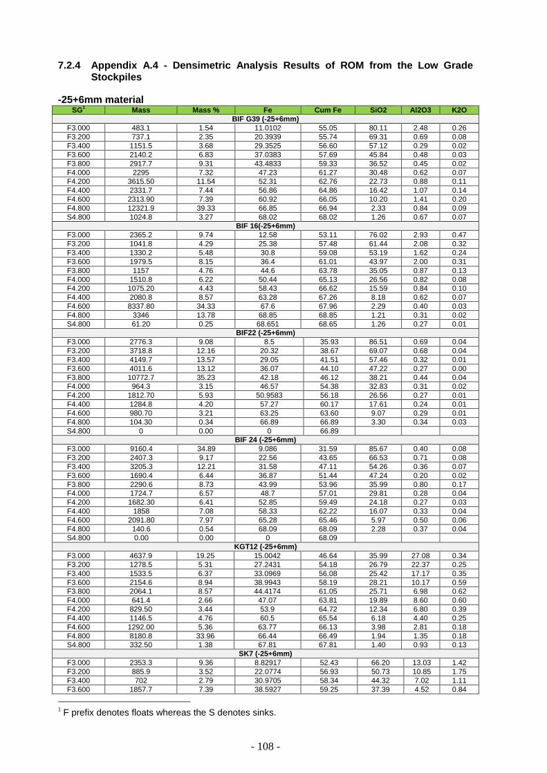
- 108 -

7.2.4 Appendix A.4 - Densimetric Analysis Results of ROM from the Low Grade Stockpiles

-25+6mm material SG

1 Mass Mass % Fe Cum Fe SiO2 Al2O3 K2O

BIF G39 (-25+6mm)

F3.000 483.1 1.54 11.0102 55.05 80.11 2.48 0.26

F3.200 737.1 2.35 20.3939 55.74 69.31 0.69 0.08

F3.400 1151.5 3.68 29.3525 56.60 57.12 0.29 0.02

F3.600 2140.2 6.83 37.0383 57.69 45.84 0.48 0.03

F3.800 2917.7 9.31 43.4833 59.33 36.52 0.45 0.02

F4.000 2295 7.32 47.23 61.27 30.48 0.62 0.07

F4.200 3615.50 11.54 52.31 62.76 22.73 0.88 0.11

F4.400 2331.7 7.44 56.86 64.86 16.42 1.07 0.14

F4.600 2313.90 7.39 60.92 66.05 10.20 1.41 0.20

F4.800 12321.9 39.33 66.85 66.94 2.33 0.84 0.09

S4.800 1024.8 3.27 68.02 68.02 1.26 0.67 0.07

BIF 16(-25+6mm)

F3.000 2365.2 9.74 12.58 53.11 76.02 2.93 0.47

F3.200 1041.8 4.29 25.38 57.48 61.44 2.08 0.32

F3.400 1330.2 5.48 30.8 59.08 53.19 1.62 0.24

F3.600 1979.5 8.15 36.4 61.01 43.97 2.00 0.31

F3.800 1157 4.76 44.6 63.78 35.05 0.87 0.13

F4.000 1510.8 6.22 50.44 65.13 26.56 0.82 0.08

F4.200 1075.20 4.43 58.43 66.62 15.59 0.84 0.10

F4.400 2080.8 8.57 63.28 67.26 8.18 0.62 0.07

F4.600 8337.80 34.33 67.6 67.96 2.29 0.40 0.03

F4.800 3346 13.78 68.85 68.85 1.21 0.31 0.02

S4.800 61.20 0.25 68.651 68.65 1.26 0.27 0.01

BIF22 (-25+6mm)

F3.000 2776.3 9.08 8.5 35.93 86.51 0.69 0.04

F3.200 3718.8 12.16 20.32 38.67 69.07 0.68 0.04

F3.400 4149.7 13.57 29.05 41.51 57.46 0.32 0.01

F3.600 4011.6 13.12 36.07 44.10 47.22 0.27 0.00

F3.800 10772.7 35.23 42.18 46.12 38.21 0.44 0.04

F4.000 964.3 3.15 46.57 54.38 32.83 0.31 0.02

F4.200 1812.70 5.93 50.9583 56.18 26.56 0.27 0.01

F4.400 1284.8 4.20 57.27 60.17 17.61 0.24 0.01

F4.600 980.70 3.21 63.25 63.60 9.07 0.29 0.01

F4.800 104.30 0.34 66.89 66.89 3.30 0.34 0.03

S4.800 0 0.00 0 66.89 BIF 24 (-25+6mm)

F3.000 9160.4 34.89 9.086 31.59 85.67 0.40 0.08

F3.200 2407.3 9.17 22.56 43.65 66.53 0.71 0.08

F3.400 3205.3 12.21 31.58 47.11 54.26 0.36 0.07

F3.600 1690.4 6.44 36.87 51.44 47.24 0.20 0.02

F3.800 2290.6 8.73 43.99 53.96 35.99 0.80 0.17

F4.000 1724.7 6.57 48.7 57.01 29.81 0.28 0.04

F4.200 1682.30 6.41 52.85 59.49 24.18 0.27 0.03

F4.400 1858 7.08 58.33 62.22 16.07 0.33 0.04

F4.600 2091.80 7.97 65.28 65.46 5.97 0.50 0.06

F4.800 140.6 0.54 68.09 68.09 2.28 0.37 0.04

S4.800 0.00 0.00 0 68.09 KGT12 (-25+6mm)

F3.000 4637.9 19.25 15.0042 46.64 35.99 27.08 0.34

F3.200 1278.5 5.31 27.2431 54.18 26.79 22.37 0.25

F3.400 1533.5 6.37 33.0969 56.08 25.42 17.17 0.35

F3.600 2154.6 8.94 38.9943 58.19 28.21 10.17 0.59

F3.800 2064.1 8.57 44.4174 61.05 25.71 6.98 0.62

F4.000 641.4 2.66 47.07 63.81 19.89 8.60 0.60

F4.200 829.50 3.44 53.9 64.72 12.34 6.80 0.39

F4.400 1146.5 4.76 60.5 65.54 6.18 4.40 0.25

F4.600 1292.00 5.36 63.77 66.13 3.98 2.81 0.18

F4.800 8180.8 33.96 66.44 66.49 1.94 1.35 0.18

S4.800 332.50 1.38 67.81 67.81 1.40 0.93 0.13

SK7 (-25+6mm)

F3.000 2353.3 9.36 8.82917 52.43 66.20 13.03 1.42

F3.200 885.9 3.52 22.0774 56.93 50.73 10.85 1.75

F3.400 702 2.79 30.9705 58.34 44.32 7.02 1.11

F3.600 1857.7 7.39 38.5927 59.25 37.39 4.52 0.84

1 F prefix denotes floats whereas the S denotes sinks.

- 109 -

SG1 Mass Mass % Fe Cum Fe SiO2 Al2O3 K2O

F3.800 2035 8.09 43.4046 61.23 31.36 4.07 0.77

F4.000 1457.8 5.80 46.48 63.33 26.69 4.19 0.85

F4.200 1307.50 5.20 54.24 64.88 17.62 2.77 0.49

F4.400 1535.1 6.11 59.0191 65.83 8.54 2.32 0.38

F4.600 2057.80 8.19 64.66 66.64 4.85 1.59 0.24

F4.800 10235.8 40.71 66.93 67.01 1.97 0.84 0.11

S4.800 712.3 2.83 68.11 68.11 1.09 0.51 0.06

SK27 (-25+6mm)

F3.000 2830.5 14.21 9.40674 52.44 44.84 29.16 0.99

F3.200 525 2.63 22.8105 59.57 36.01 21.84 0.52

F3.400 526.4 2.64 29.716 60.73 28.69 20.06 0.48

F3.600 816.1 4.10 37.0817 61.75 23.26 16.49 0.26

F3.800 795.9 3.99 42.9983 63.07 17.96 13.56 0.20

F4.000 793.5 3.98 49.0555 64.18 14.46 10.49 0.17

F4.200 719.00 3.61 54.23 65.06 11.02 7.79 0.13

F4.400 1385 6.95 59.52 65.66 7.40 5.06 0.13

F4.600 2303.30 11.56 64.18 66.40 4.51 2.49 0.08

F4.800 7691.4 38.60 66.71 66.95 2.37 1.08 0.02

S4.800 1538.90 7.72 68.15 68.15 1.48 0.67 0.01

SK30 (-25+6mm)

F3.000 158 1.19 16.0913 53.32 37.57 26.54 0.80

F3.200 218 1.65 26.25 53.77 28.66 22.99 0.74

F3.400 402.5 3.04 31.59 54.23 24.43 20.67 0.57

F3.600 629 4.75 38.24 54.96 20.53 17.17 0.43

F3.800 1446.6 10.93 44.23 55.85 16.29 14.26 0.31

F4.000 1731.2 13.09 48.929 57.47 12.80 12.05 0.28

F4.200 2235.00 16.89 55.1662 59.19 9.48 7.69 0.13

F4.400 3790.8 28.66 58.66 60.59 6.82 5.84 0.08

F4.600 2475.50 18.71 63.24 63.38 4.98 3.27 0.03

F4.800 142.5 1.08 65.8 65.80 3.64 1.99 0.02

S4.800 0 0.00 0 65.80

-6+2mm material SG Mass Mass % Fe Cum Fe SiO2 Al2O3 K2O

BIF G39 (-6+2mm)

F3.000 768.9 3.79 9.507 53.90 77.22 5.59 0.46

F3.200 921 4.54 19.88 55.65 66.91 2.47 0.28

F3.400 858.4 4.23 30.858 57.42 53.81 0.99 0.11

F3.600 1187.9 5.85 38.920 58.70 42.81 0.66 0.06

F3.800 2502.4 12.33 48.968 60.12 28.21 0.79 0.08

F4.000 1054.4 5.20 44.21 62.11 34.08 0.86 0.10

F4.200 1887 9.30 56.12 63.56 17.05 0.93 0.12

F4.400 2461.6 12.13 60.54 64.83 11.08 0.97 0.12

F4.600 2828.2 13.94 64.71 66.05 4.93 0.91 0.09

F4.800 5116.2 25.22 66.59 66.69 2.69 0.83 0.07

S4.800 703.5 3.47 67.45 67.45 1.90 0.72 0.05

BIF 16 (-6+2mm)

F3.000 2879.4 13.24 11.2663 51.42 77.07 3.80 0.58

F3.200 1529.3 7.03 25.9033 57.55 57.95 2.66 0.56

F3.400 964.9 4.44 31.6846 60.35 50.11 2.50 0.46

F3.600 977.9 4.50 37.9269 62.04 40.04 3.17 0.38

F3.800 2610.1 12.00 57.0173 63.57 15.13 0.99 0.14

F4.000 883.1 4.06 45.59 64.90 32.50 1.82 0.25

F4.200 1490.7 6.86 60.26 66.34 12.34 0.86 0.11

F4.400 2797.6 12.87 65.5 67.21 4.90 0.58 0.06

F4.600 4831.4 22.22 67.69 67.84 2.27 0.51 0.04

F4.800 2729.8 12.55 68.09 68.09 1.71 0.47 0.04

S4.800 50 0.23 68.08 68.08 1.51 0.57 0.03

BIF22 (-6+2mm)

F3.000 8346.1 41.68 8.275 27.38 86.78 0.76 0.04

F3.200 2051.2 10.24 20.91 41.03 69.10 0.44 0.02

F3.400 2258.9 11.28 30.58 45.32 56.04 0.38 0.02

F3.600 1856.7 9.27 38.6 49.83 44.47 0.61 0.06

F3.800 1945.2 9.71 44.9 53.62 35.02 0.54 0.02

F4.000 634.6 3.17 51.046 58.37 26.52 0.33 0.01

F4.200 1151.5 5.75 55.33 59.96 19.39 0.41 0.01

F4.400 1199.1 5.99 61.78 62.95 10.83 0.38 0.01

F4.600 571.8 2.86 65.34 65.35 5.51 0.32 0.01

F4.800 10.6 0.05 65.63 65.63 5.57 0.32 0.00

S4.800 0 0.00 0 65.63 BIF 24 (-6+2mm)

F3.000 7374.7 35.56 7.79013 33.51 87.42 0.81 0.13

F3.200 1608.5 7.76 21.85 47.70 66.11 0.96 0.16

F3.400 1796.2 8.66 31.21 51.24 53.99 0.83 0.13

- 110 -

SG Mass Mass % Fe Cum Fe SiO2 Al2O3 K2O

F3.600 1403.3 6.77 40.05 54.85 40.46 0.72 0.10

F3.800 2265.4 10.92 50.03 57.28 26.38 0.59 0.08

F4.000 838.2 4.04 42.59 59.89 38.17 0.50 0.07

F4.200 1286.9 6.21 55.51 62.55 19.46 0.47 0.07

F4.400 1300.6 6.27 61.34 64.72 11.14 0.60 0.09

F4.600 2803.4 13.52 66.26 66.26 3.95 0.60 0.08

F4.800 59.7 0.29 66.38 66.38 3.19 0.69 0.09

S4.800 0 0.00 0 66.38 KGT12 (-6+2mm)

F3.000 3960.6 18.94 13.0709 45.29 36.98 27.31 0.37

F3.200 1367.8 6.54 24.4263 52.81 28.69 22.58 0.35

F3.400 1556.1 7.44 32.9424 55.31 24.76 17.44 0.37

F3.600 2463.8 11.78 40.7674 57.79 25.12 10.09 0.54

F3.800 2103.5 10.06 48.7044 61.42 16.93 8.16 0.39

F4.000 1005.2 4.81 52.7782 64.24 13.96 6.83 0.34

F4.200 1339.4 6.41 60.7629 65.61 6.62 4.25 0.21

F4.400 1889.9 9.04 64.8212 66.52 3.49 2.41 0.18

F4.600 2391.3 11.44 66.7065 67.14 2.15 1.49 0.15

F4.800 2730.8 13.06 67.4903 67.50 1.72 1.18 0.14

S4.800 99.6 0.48 67.7304 67.73 1.48 0.99 0.12

SK7 (-6+2mm)

F3.000 2844.5 12.00 8.29929 51.70 65.22 14.36 1.51

F3.200 902.2 3.81 22.176 57.62 49.10 12.45 1.93

F3.400 739 3.12 31.7016 59.22 41.83 8.12 1.36

F3.600 1801.3 7.60 39.2213 60.28 33.43 6.53 1.14

F3.800 2201.7 9.29 48.912 62.45 21.99 4.62 0.90

F4.000 1187.8 5.01 50.17 64.41 20.97 4.13 0.75

F4.200 1877.9 7.92 59.97 65.62 9.46 2.48 0.42

F4.400 3206.2 13.52 64.3978 66.49 5.05 1.69 0.25

F4.600 4239.4 17.88 66.6661 67.24 2.58 1.19 0.17

F4.800 4540.7 19.15 67.7479 67.76 1.60 0.83 0.10

S4.800 168.3 0.71 68.0327 68.03 1.46 0.62 0.08

SK27 (-6+2mm)

F3.000 3361.8 14.60 8.521 52.31 45.25 29.66 0.95

F3.200 673.5 2.92 22.22 59.80 37.04 21.51 0.50

F3.400 602 2.61 32.13 61.13 27.96 18.37 0.33

F3.600 951.6 4.13 40.03 62.08 21.28 15.07 0.27

F3.800 2092.2 9.08 52.7 63.29 12.09 8.48 0.14

F4.000 1503.4 6.53 55.14 64.73 10.80 6.36 0.12

F4.200 1925.3 8.36 60.9 65.77 6.08 3.86 0.07

F4.400 2447.6 10.63 65.248 66.56 3.50 2.02 0.04

F4.600 3594.8 15.61 66.12 66.89 2.93 1.38 0.02

F4.800 5734.9 24.90 67.37 67.37 1.99 1.02 0.03

S4.800 143.2 0.62 67.23 67.23 2.01 1.03 0.03

SK30 (-6+2mm)

F3.000 336 2.40 12.2947 51.55 40.01 28.38 1.14

F3.200 401.4 2.87 24.83 52.51 29.13 23.89 0.77

F3.400 696.6 4.97 32.43 53.35 23.77 20.48 0.58

F3.600 1735.2 12.39 42.37 54.51 17.32 15.40 0.38

F3.800 1919 13.70 50.2 56.45 12.20 11.31 0.25

F4.000 2202.9 15.73 50.89 57.80 11.39 10.35 0.21

F4.200 2594.2 18.52 56.38 60.06 7.93 7.60 0.13

F4.400 1830.1 13.07 60.53 62.38 5.52 5.16 0.08

F4.600 2241.7 16.01 63.86 63.87 3.83 3.22 0.04

F4.800 48 0.34 64.15 64.15 3.62 2.89 0.04

S4.800 0 0.00 0 64.15

- 111 -

7.2.5 Appendix A.5 - Chemical and Densimetric Analysis Results of Material Treated through the Ultra-High Density DMS

Low Grade Stockpile Material

14/01 Day Shift Feed Mass (g) Mass (%) Fe SiO2 Al2O3 K2O

U1-14DS Feed F3.62 2983.5 25.69 15.3 52.5 16.09 2.56

U1-14DS Feed F3.8 371.4 3.20 38.4 26.0 10.78 1.80

U1-14DS Feed F4.0 544.3 4.69 45.5 19.3 8.93 1.31

U1-14DS Feed F4.2 491.5 4.23 51.3 14.0 7.49 0.99

U1-14DS Feed F4.4 847.8 7.30 55.6 10.0 5.81 0.79

U1-14DS Feed F4.6 1150.5 9.91 60.5 6.0 3.92 0.48

U1-14DS Feed F4.8 2021.9 17.41 64.4 3.4 2.26 0.28

U1-14DS Feed F5.0 2152.4 18.53 67.0 1.76 1.15 0.13

U1-14DS Feed S5.0 1051.3 9.05 68.5 1.08 0.71 0.07

14/01 Day Shift Product Mass (g) Mass (%) Fe SiO2 Al2O3 K2O

U2-14DS Product F4.2 124 0.91 48.7 16.9 8.10 1.18

U2-14DS Product F4.4 160.7 1.18 55.9 9.6 5.92 0.79

U2-14DS Product F4.6 695.5 5.12 61.2 5.8 3.70 0.46

U2-14DS Product F4.8 4363 32.11 65.1 3.1 2.08 0.25

U2-14DS Product F5.0 5790.4 42.62 66.9 1.77 1.10 0.12

U2-14DS Product S5.0 2452.7 18.05 68.1 1.06 0.49 0.06

14/01 Day Shift Waste Mass (g) Mass (%) Fe SiO2 Al2O3 K2O

U3-14DS Waste F3.6 5478.6 42.67 14.9 52.6 16.71 2.76

U3-14DS Waste F3.8 893.4 6.96 40.3 24.3 10.50 1.65

U3-14DS Waste F4.0 541.6 4.22 45.6 19.0 9.00 1.35

U3-14DS Waste F4.2 1141.5 8.89 50.5 14.3 7.66 1.07

U3-14DS Waste F4.4 1330.6 10.36 56.0 9.9 5.73 0.76

U3-14DS Waste F4.6 2070.2 16.12 61.5 5.3 3.36 0.44

U3-14DS Waste F4.8 1140 8.88 63.1 4.55 2.95 0.38

U3-14DS Waste S4.8 244.7 1.91 66.8 2.06 1.45 0.16

14/01 Night Shift Feed Mass (g) Mass (%) Fe SiO2 Al2O3 K2O

U4-14NS Feed F3.6 3293.5 24.73 14.4 51.3 16.04 2.57

U4-14NS Feed F3.8 628.4 4.72 39.8 26.0 10.51 1.68

U4-14NS Feed F4.0 423 3.18 46.0 18.8 8.61 1.33

U4-14NS Feed F4.2 723.4 5.43 51.3 14.3 7.34 1.03

U4-14NS Feed F4.4 836.2 6.28 55.8 10.2 5.82 0.80

U4-14NS Feed F4.6 1104.1 8.29 60.5 6.3 3.96 0.52

U4-14NS Feed F4.8 1846.4 13.86 64.4 3.6 2.31 0.29

U4-14NS Feed F5.0 2850.3 21.40 66.6 2.00 1.32 0.16

U4-14NS Feed S5.0 1614.7 12.12 68.4 1.22 0.79 0.08

14/01 Night Shift Product Mass (g) Mass (%) Fe SiO2 Al2O3 K2O

U5-14NS Product F4.2 115 0.81 46.9 18.9 8.60 1.26

U5-14NS Product F4.4 190 1.35 54.9 10.8 6.08 0.76

U5-14NS Product F4.6 1357.7 9.62 63.3 4.6 3.00 0.38

U5-14NS Product F4.8 4326.4 30.65 64.7 3.1 2.08 0.25

U5-14NS Product F5.0 5055.1 35.81 67.6 1.64 1.10 0.12

U5-14NS Product S5.0 3072.3 21.76 68.6 1.17 0.77 0.07

14/01 Night Shift Waste Mass (g) Mass (%) Fe SiO2 Al2O3 K2O

U6-14NS Waste F3.6 6103.5 44.77 15.2 52.2 16.59 2.65

U6-14NS Waste F3.8 657.3 4.82 38.8 26.3 10.69 1.66

U6-14NS Waste F4.0 852.6 6.25 45.2 20.0 9.15 1.38

U6-14NS Waste F4.2 1135.9 8.33 51.8 13.6 7.34 1.05

U6-14NS Waste F4.4 1295 9.50 55.0 10.6 6.05 0.81

U6-14NS Waste F4.6 2172 15.93 60.5 6.1 3.81 0.51

U6-14NS Waste F4.8 906.2 6.65 63.9 3.4 2.23 0.30

U6-14NS Waste F5.0 405.1 2.97 66.3 2.47 1.63 0.21

U6-14NS Waste S5.0 105 0.77 67.6 1.79 1.17 0.13

2 F prefix on the number denotes float at that particular density, whereas S prefix denotes sinks

- 112 -

Jig Waste Material

15/01 Day Shift Feed Mass (g) Mass (%) Fe SiO2 Al2O3 K2O

U7-15DS Feed F3.6 5038.7 38.41 16.5 63.5 8.25 0.99

U7-15DS Feed F3.8 580.2 4.42 40.2 33.5 4.89 0.68

U7-15DS Feed F4.0 543.8 4.15 45.6 26.9 4.15 0.52

U7-15DS Feed F4.2 756.9 5.77 53.1 17.0 3.61 0.46

U7-15DS Feed F4.4 659.4 5.03 58.6 10.3 2.41 0.32

U7-15DS Feed F4.6 1168.8 8.91 60.4 7.9 2.11 0.30

U7-15DS Feed F4.8 1645.8 12.55 66.1 2.7 1.01 0.15

U7-15DS Feed F5.0 1633.7 12.45 66.5 2.11 0.87 0.12

U7-15DS Feed S5.0 1090 8.31 67.5 1.30 0.59 0.07

15/01 Day Shift Product Mass (g) Mass (%) Fe SiO2 Al2O3 K2O

U8-15DS Product F4.2 267.3 1.80 46.7 24.5 4.06 0.55

U8-15DS Product F4.4 185.2 1.25 55.5 14.0 3.19 0.41

U8-15DS Product F4.6 541.7 3.65 61.1 7.2 1.97 0.29

U8-15DS Product F4.8 3553.9 23.96 65.5 3.2 1.20 0.18

U8-15DS Product F5.0 7070.5 47.67 67.2 1.54 0.66 0.08

U8-15DS Product S5.0 3212.6 21.66 67.7 1.02 0.49 0.05

15/01 Day Shift Waste Mass (g) Mass (%) Fe SiO2 Al2O3 K2O

U9-15DS Waste F3.6 5936.5 52.65 16.8 61.8 8.34 1.00

U9-15DS Waste F3.8 639.8 5.67 40.9 32.8 4.55 0.63

U9-15DS Waste F4.0 564.3 5.00 46.4 25.3 4.19 0.56

U9-15DS Waste F4.2 746.2 6.62 53.2 16.6 3.59 0.48

U9-15DS Waste F4.4 949.8 8.42 56.0 13.3 3.11 0.41

U9-15DS Waste F4.6 879.4 7.80 62.4 5.9 1.80 0.26

U9-15DS Waste F4.8 1144.8 10.15 64.4 4.01 1.36 0.20

U9-15DS Waste S4.8 414.9 3.68 67.3 1.70 0.71 0.09

- 113 -

APPENDIX B: FESI CHARACTERISATION

7.2.6 Appendix B.1 - Viscosity Modifier Specification

Test Method Dry matter % 52.0 ± 2.0 LAB TEST 001 pH (10% Solution) 7.0 ± 0.8 LAB TEST 008 Insolubles % Max 0.5 LAB TEST 004

Parameter Typical values* pH 6.8 Calcium 6.0% Total Sulphur 4.0% Reducing Sugars 2.0% HPLC Sugars <1.0% Alkaline Content ≤ 0.50% m/m Chloride Content ≤ 0.10% m/m

LignoTech SA

Umkomanzi Drift P.O. Box 743

Umkomaas 4170 South Africa

Tel: +27 (0) 39 97 36 000

Fax: +27 (0) 39 97 36 015 DP 725

Spec. No.: 013 Effective Date: 12.12.06

Revision Date: 03.08.10 Revision No. : 03

DP 725

Product Description

DP 725 is a purified grade calcium lignosulphonate product with low insoluble content and with near neutral pH.

Typical application: As plasticizer or water reducing admixture for good grade concrete and mortar. When used as admixture, it reduces water demand, improves workability and produce low air entrained concrete, mortar.

CAS No. 8061-52-7 (Calcium lignosulphonate)

Specifications

Active customers would be notified of changes where any.

Chemical Data Physical Data

Parameter Typical values* Colour Brown Dry Matter 51% Density(51% DS, 25 0C) 1270 kg/m3

*The above analyses are not formal specifications and values may change. All values calculated on solids where appli-

cable.

Storage Stability:

As this is a liquid product, shelf life may vary from a few months to about 6 months dependent upon the storage condition when kept in the original sealed packaging or tank. No preservative has been added additionally.

Compatibility:

Lignosulphonates are compatible with anionic and non-ionic dispersants, wetting agents and most organic and inorganic materials.

Delivery Form:

Liquid product is available in flowbins or bulk truckloads. Alternative forms available upon further discussion.

Lead Time:

2 weeks lead time is typical for local. 6 to 8 weeks lead time for international.

Material Safety Data Sheets are available upon request. UNCONTROLLED COPY Please contact your LignoTech Sales Representative for additional product information.

The information given here is based on our best knowledge and we believe it to be true and accurate. However, LignoTech South Africa does not

warrant or guarantee in any manner whatsoever, including the warranty of merchant-ability or fitness for the end user the accuracy of the informa-

tion and procedures listed herein and will not be responsible for any damage resulting from their use.

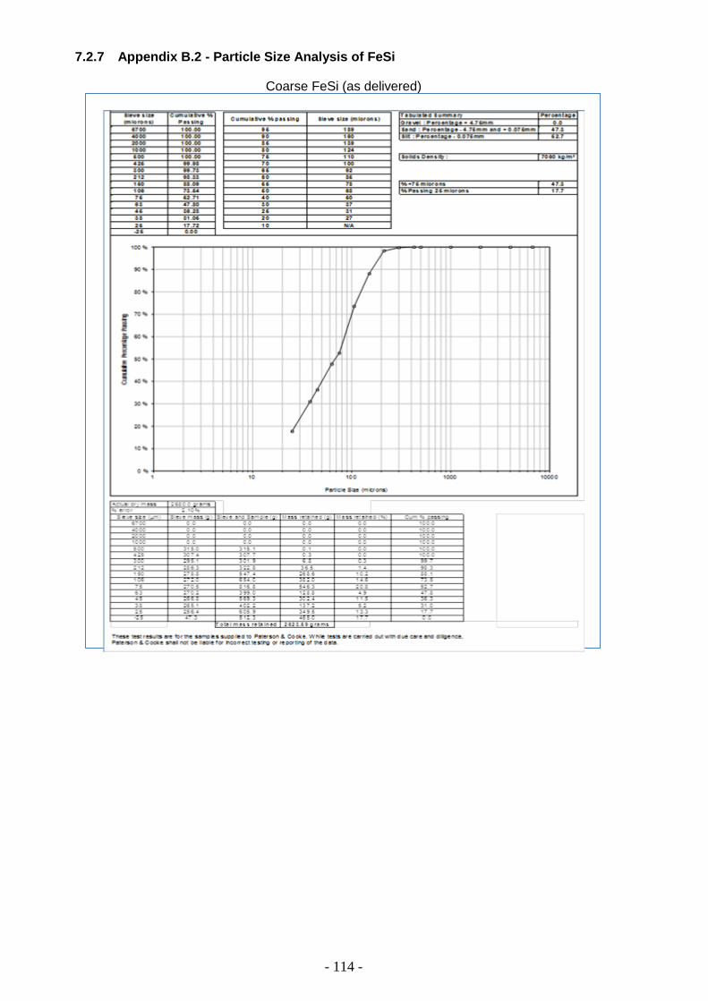
- 114 -

7.2.7 Appendix B.2 - Particle Size Analysis of FeSi

Coarse FeSi (as delivered)

- 115 -

Coarse FeSi less Fines

- 116 -

Process FeSi (as delivered)

- 117 -

Process FeSi less Fines

- 118 -

7.2.8 Appendix B.3 - Pipe Loop Settling Data

Material Density

Coarse FeSi Less Fines

3604 kg/m3

3938 kg/m3

4135 kg/m3

4233 kg/m3

Process FeSi

3991 kg/m3

3898 kg/m3

3822 kg/m3

3609 kg/m3

3609 kg/m3

Process FeSi Less Fines

3991 kg/m3

3898 kg/m3

3822 kg/m3

3609 kg/m3

Coarse FeSi with Rheology Modifier

3704 kg/m3

3915 kg/m3

4085 kg/m3

4251 kg/m3

NB! Appended data for only a single density for each dense medium type tested, however, detailed data available for all density range tested. Coarse FeSi Less Fines

3604 kg/m³

Data point Pressure Bottom - kPa (abs) Pressure Top - kPa (abs) Density Calc Duration

8 167.748 132.396 3604 kg/m³ 00:00:00

9 167.484 132.114 3606 kg/m³ 00:00:04

10 167.391 131.906 3617 kg/m³ 00:00:08

11 167.246 131.801 3613 kg/m³ 00:00:12

12 167.112 131.656 3614 kg/m³ 00:00:16

13 167.009 131.461 3624 kg/m³ 00:00:20

14 166.921 131.338 3627 kg/m³ 00:00:24

15 166.784 131.228 3624 kg/m³ 00:00:28

16 166.726 131.027 3639 kg/m³ 00:00:32

17 166.620 130.887 3642 kg/m³ 00:00:37

18 166.470 130.688 3648 kg/m³ 00:00:41

19 166.405 130.556 3654 kg/m³ 00:00:46

20 166.299 130.495 3650 kg/m³ 00:00:50

21 166.219 130.315 3660 kg/m³ 00:00:54

22 166.176 130.114 3676 kg/m³ 00:00:59

23 166.083 130.025 3676 kg/m³ 00:01:03

24 166.057 129.940 3682 kg/m³ 00:01:07

25 165.826 129.757 3677 kg/m³ 00:01:12

26 165.632 129.644 3669 kg/m³ 00:01:16

27 165.288 129.470 3651 kg/m³ 00:01:20

28 165.118 129.342 3647 kg/m³ 00:01:25

29 164.669 129.238 3612 kg/m³ 00:01:29

30 164.333 129.112 3590 kg/m³ 00:01:33

31 164.090 129.015 3576 kg/m³ 00:01:37

32 163.869 128.907 3564 kg/m³ 00:01:41

33 163.536 128.795 3541 kg/m³ 00:01:45

34 163.224 128.657 3524 kg/m³ 00:01:49

35 162.928 128.514 3508 kg/m³ 00:01:53

36 162.684 128.456 3489 kg/m³ 00:01:57

- 119 -


37 162.411 128.273 3480 kg/m³ 00:02:01

38 162.128 128.168 3462 kg/m³ 00:02:05

39 161.842 128.080 3442 kg/m³ 00:02:09

40 161.521 127.998 3417 kg/m³ 00:02:13

41 161.248 127.896 3400 kg/m³ 00:02:17

42 160.962 127.797 3381 kg/m³ 00:02:21

43 160.672 127.628 3368 kg/m³ 00:02:25

44 160.394 127.566 3346 kg/m³ 00:02:29

45 160.202 127.442 3339 kg/m³ 00:02:33

46 159.862 127.421 3307 kg/m³ 00:02:37

47 159.579 127.311 3289 kg/m³ 00:02:41

48 159.318 127.164 3278 kg/m³ 00:02:45

49 159.061 127.083 3260 kg/m³ 00:02:49

50 158.762 126.943 3243 kg/m³ 00:02:53

51 158.467 126.894 3218 kg/m³ 00:02:57

52 158.210 126.765 3205 kg/m³ 00:03:01

53 157.917 126.683 3184 kg/m³ 00:03:05

54 157.691 126.597 3170 kg/m³ 00:03:09

55 157.362 126.470 3149 kg/m³ 00:03:14

56 157.084 126.361 3132 kg/m³ 00:03:18

57 156.800 126.250 3114 kg/m³ 00:03:23

58 156.478 126.160 3091 kg/m³ 00:03:27

59 156.161 126.060 3068 kg/m³ 00:03:31

60 155.916 125.985 3051 kg/m³ 00:03:35

61 155.641 125.889 3033 kg/m³ 00:03:39

62 155.431 125.789 3022 kg/m³ 00:03:43

63 155.131 125.752 2995 kg/m³ 00:03:47

64 154.857 125.643 2978 kg/m³ 00:03:51

65 154.641 125.583 2962 kg/m³ 00:03:55

66 154.356 125.460 2946 kg/m³ 00:03:59

67 154.076 125.384 2925 kg/m³ 00:04:03

68 153.854 125.287 2912 kg/m³ 00:04:07

69 153.587 125.210 2893 kg/m³ 00:04:11

70 153.291 125.158 2868 kg/m³ 00:04:15

71 153.055 125.040 2856 kg/m³ 00:04:19

72 152.807 125.008 2834 kg/m³ 00:04:23

73 152.551 124.809 2828 kg/m³ 00:04:27

74 152.308 124.801 2804 kg/m³ 00:04:31

75 152.068 124.732 2787 kg/m³ 00:04:35

76 151.795 124.713 2761 kg/m³ 00:04:39

77 151.574 124.589 2751 kg/m³ 00:04:43

78 151.287 124.558 2725 kg/m³ 00:04:47

79 151.069 124.441 2714 kg/m³ 00:04:51

80 150.799 124.367 2694 kg/m³ 00:04:55

81 150.534 124.219 2682 kg/m³ 00:04:59

82 150.308 124.141 2667 kg/m³ 00:05:03

83 150.093 124.112 2648 kg/m³ 00:05:07

84 149.799 124.044 2625 kg/m³ 00:05:11

85 149.583 124.002 2608 kg/m³ 00:05:15

86 149.360 123.947 2591 kg/m³ 00:05:19

87 149.099 123.900 2569 kg/m³ 00:05:23

88 148.826 123.747 2556 kg/m³ 00:05:27

89 148.630 123.725 2539 kg/m³ 00:05:31

90 148.416 123.663 2523 kg/m³ 00:05:35

- 120 -


91 148.221 123.578 2512 kg/m³ 00:05:39

92 147.948 123.503 2492 kg/m³ 00:05:43

93 147.724 123.445 2475 kg/m³ 00:05:47

94 147.472 123.353 2459 kg/m³ 00:05:51

95 147.233 123.287 2441 kg/m³ 00:05:55

96 147.062 123.254 2427 kg/m³ 00:05:59

97 146.795 123.145 2411 kg/m³ 00:06:03

98 146.566 123.114 2391 kg/m³ 00:06:07

99 146.391 123.009 2384 kg/m³ 00:06:11

100 146.195 122.933 2371 kg/m³ 00:06:15

101 145.939 122.903 2348 kg/m³ 00:06:19

102 145.754 122.858 2334 kg/m³ 00:06:23

103 145.522 122.781 2318 kg/m³ 00:06:27

104 145.306 122.673 2307 kg/m³ 00:06:31

105 145.091 122.660 2286 kg/m³ 00:06:35

106 144.819 122.566 2268 kg/m³ 00:06:39

107 144.620 122.544 2250 kg/m³ 00:06:43

108 144.455 122.496 2238 kg/m³ 00:06:47

109 144.270 122.418 2228 kg/m³ 00:06:51

110 144.064 122.361 2212 kg/m³ 00:06:55

111 143.862 122.295 2199 kg/m³ 00:06:59

112 143.671 122.274 2181 kg/m³ 00:07:03

113 143.523 122.180 2176 kg/m³ 00:07:07

114 143.323 122.127 2161 kg/m³ 00:07:11

115 143.126 122.099 2143 kg/m³ 00:07:15

116 143.072 122.019 2146 kg/m³ 00:07:19

117 142.915 121.976 2134 kg/m³ 00:07:23

118 142.852 121.897 2136 kg/m³ 00:07:27

119 142.693 121.864 2123 kg/m³ 00:07:31

120 142.537 121.790 2115 kg/m³ 00:07:35

121 142.397 121.772 2102 kg/m³ 00:07:39

122 142.304 121.740 2096 kg/m³ 00:07:43

123 142.030 121.651 2077 kg/m³ 00:07:47

124 141.718 121.624 2048 kg/m³ 00:07:51

125 141.477 121.589 2027 kg/m³ 00:07:55

126 141.175 121.479 2008 kg/m³ 00:07:59

127 140.877 121.464 1979 kg/m³ 00:08:03

128 140.584 121.434 1952 kg/m³ 00:08:07

129 140.360 121.340 1939 kg/m³ 00:08:11

130 140.088 121.311 1914 kg/m³ 00:08:15

131 139.852 121.263 1895 kg/m³ 00:08:19

132 139.692 121.233 1882 kg/m³ 00:08:23

133 139.499 121.214 1864 kg/m³ 00:08:27

134 139.209 121.161 1840 kg/m³ 00:08:31

135 139.060 121.046 1836 kg/m³ 00:08:35

136 138.860 121.030 1818 kg/m³ 00:08:39

137 138.630 120.993 1798 kg/m³ 00:08:43

138 138.455 120.933 1786 kg/m³ 00:08:47

139 138.275 120.895 1772 kg/m³ 00:08:51

140 138.104 120.870 1757 kg/m³ 00:08:55

141 137.953 120.806 1748 kg/m³ 00:08:59

142 137.747 120.726 1735 kg/m³ 00:09:03

143 137.594 120.716 1720 kg/m³ 00:09:07

144 137.459 120.670 1711 kg/m³ 00:09:11

- 121 -


145 137.243 120.667 1690 kg/m³ 00:09:15

146 137.095 120.594 1682 kg/m³ 00:09:19

147 136.946 120.593 1667 kg/m³ 00:09:23

148 136.815 120.516 1661 kg/m³ 00:09:27

149 136.664 120.505 1647 kg/m³ 00:09:31

150 136.620 120.463 1647 kg/m³ 00:09:35

151 136.530 120.419 1642 kg/m³ 00:09:39

152 136.735 120.389 1666 kg/m³ 00:09:43

153 147.855 120.337 2805 kg/m³ 00:09:47

154 155.313 120.308 3568 kg/m³ 00:09:51

155 156.121 120.222 3659 kg/m³ 00:09:55

156 156.016 120.172 3654 kg/m³ 00:09:59

157 155.069 120.108 3564 kg/m³ 00:10:03

Process FeSi

3350 kg/m3


7 166.999 134.138 3350 kg/m³ 00:00:00

8 167.688 134.403 3393 kg/m³ 00:00:04

9 168.059 134.513 3420 kg/m³ 00:00:08

10 168.151 134.540 3426 kg/m³ 00:00:12

11 168.135 134.481 3431 kg/m³ 00:00:16

12 168.205 134.490 3437 kg/m³ 00:00:20

13 168.244 134.480 3442 kg/m³ 00:00:24

14 168.236 134.456 3443 kg/m³ 00:00:28

15 168.303 134.410 3455 kg/m³ 00:00:32

16 168.319 134.395 3458 kg/m³ 00:00:36

17 168.237 134.390 3450 kg/m³ 00:00:40

18 168.244 134.358 3454 kg/m³ 00:00:44

19 168.228 134.395 3449 kg/m³ 00:00:48

20 168.287 134.368 3458 kg/m³ 00:00:52

21 168.255 134.358 3455 kg/m³ 00:00:56

22 168.251 134.354 3455 kg/m³ 00:01:00

23 168.238 134.348 3455 kg/m³ 00:01:04

24 168.270 134.318 3461 kg/m³ 00:01:08

25 168.296 134.250 3471 kg/m³ 00:01:12

26 168.279 134.237 3470 kg/m³ 00:01:16

27 168.262 134.193 3473 kg/m³ 00:01:20

28 168.222 134.194 3469 kg/m³ 00:01:24

29 168.234 134.129 3477 kg/m³ 00:01:28

30 168.363 134.159 3487 kg/m³ 00:01:32

31 167.974 134.034 3460 kg/m³ 00:01:36

32 168.154 134.080 3473 kg/m³ 00:01:40

33 168.274 134.103 3483 kg/m³ 00:01:44

34 168.176 134.027 3481 kg/m³ 00:01:48

35 168.101 134.005 3476 kg/m³ 00:01:52

36 168.110 134.059 3471 kg/m³ 00:01:56

37 168.111 134.118 3465 kg/m³ 00:02:00

38 168.128 134.095 3469 kg/m³ 00:02:04

39 168.115 134.164 3461 kg/m³ 00:02:08

40 168.082 134.066 3467 kg/m³ 00:02:12

41 168.048 134.054 3465 kg/m³ 00:02:16

42 167.987 134.065 3458 kg/m³ 00:02:20

43 168.013 134.043 3463 kg/m³ 00:02:24

- 122 -


44 167.950 134.074 3453 kg/m³ 00:02:28

45 167.926 133.984 3460 kg/m³ 00:02:32

46 167.922 133.961 3462 kg/m³ 00:02:36

47 167.891 133.926 3462 kg/m³ 00:02:40

48 167.824 133.888 3459 kg/m³ 00:02:44

49 167.858 133.864 3465 kg/m³ 00:02:48

50 167.813 133.919 3455 kg/m³ 00:02:52

51 167.807 133.836 3463 kg/m³ 00:02:56

52 167.810 133.844 3462 kg/m³ 00:03:00

53 167.774 133.803 3463 kg/m³ 00:03:04

54 167.783 133.746 3470 kg/m³ 00:03:08

55 167.792 133.716 3474 kg/m³ 00:03:12

56 167.758 133.681 3474 kg/m³ 00:03:16

57 167.793 133.653 3480 kg/m³ 00:03:20

58 167.766 133.707 3472 kg/m³ 00:03:24

59 167.799 133.608 3485 kg/m³ 00:03:28

60 167.741 133.638 3476 kg/m³ 00:03:32

61 167.726 133.663 3472 kg/m³ 00:03:36

62 167.728 133.638 3475 kg/m³ 00:03:40

63 167.676 133.664 3467 kg/m³ 00:03:44

64 167.655 133.751 3456 kg/m³ 00:03:48

65 167.589 133.754 3449 kg/m³ 00:03:52

66 167.601 133.748 3451 kg/m³ 00:03:56

67 167.596 133.712 3454 kg/m³ 00:04:00

68 167.509 133.711 3445 kg/m³ 00:04:04

69 167.509 133.659 3451 kg/m³ 00:04:08

70 167.455 133.666 3444 kg/m³ 00:04:12

71 167.428 133.642 3444 kg/m³ 00:04:16

72 167.419 133.591 3448 kg/m³ 00:04:20

73 167.349 133.661 3434 kg/m³ 00:04:24

74 167.344 133.617 3438 kg/m³ 00:04:28

75 167.288 133.587 3435 kg/m³ 00:04:32

76 167.284 133.499 3444 kg/m³ 00:04:36

77 167.220 133.506 3437 kg/m³ 00:04:40

78 167.229 133.489 3439 kg/m³ 00:04:44

79 167.140 133.479 3431 kg/m³ 00:04:48

80 167.104 133.455 3430 kg/m³ 00:04:52

81 167.023 133.448 3423 kg/m³ 00:04:56

82 166.961 133.442 3417 kg/m³ 00:05:00

83 166.918 133.382 3418 kg/m³ 00:05:04

84 166.867 133.383 3413 kg/m³ 00:05:08

85 166.837 133.329 3416 kg/m³ 00:05:12

86 166.741 133.350 3404 kg/m³ 00:05:16

87 166.714 133.299 3406 kg/m³ 00:05:20

88 166.609 133.335 3392 kg/m³ 00:05:24

89 166.545 133.285 3390 kg/m³ 00:05:28

90 166.555 133.294 3391 kg/m³ 00:05:32

91 166.490 133.225 3391 kg/m³ 00:05:36

92 166.490 133.234 3390 kg/m³ 00:05:40

93 166.447 133.226 3386 kg/m³ 00:05:44

94 166.338 133.221 3376 kg/m³ 00:05:48

95 166.265 133.247 3366 kg/m³ 00:05:52

96 166.227 133.179 3369 kg/m³ 00:05:56

97 166.181 133.183 3364 kg/m³ 00:06:00

98 166.072 133.224 3348 kg/m³ 00:06:04

- 123 -


99 166.028 133.210 3345 kg/m³ 00:06:08

100 165.996 133.143 3349 kg/m³ 00:06:12

101 165.925 133.148 3341 kg/m³ 00:06:16

102 165.887 133.175 3335 kg/m³ 00:06:20

103 165.806 133.108 3333 kg/m³ 00:06:24

104 165.699 133.083 3325 kg/m³ 00:06:28

105 165.687 133.097 3322 kg/m³ 00:06:32

106 165.680 133.049 3326 kg/m³ 00:06:36

107 165.552 132.996 3319 kg/m³ 00:06:40

108 165.484 132.984 3313 kg/m³ 00:06:44

109 165.409 132.974 3306 kg/m³ 00:06:48

110 165.339 132.969 3300 kg/m³ 00:06:52

111 165.272 132.957 3294 kg/m³ 00:06:56

112 165.203 132.952 3288 kg/m³ 00:07:00

113 165.178 132.911 3289 kg/m³ 00:07:04

114 165.046 132.909 3276 kg/m³ 00:07:08

115 165.053 132.861 3282 kg/m³ 00:07:12

116 164.944 132.887 3268 kg/m³ 00:07:16

117 164.837 132.874 3258 kg/m³ 00:07:20

118 164.821 132.847 3259 kg/m³ 00:07:24

119 164.756 132.859 3251 kg/m³ 00:07:28

120 164.680 132.796 3250 kg/m³ 00:07:32

121 164.616 132.820 3241 kg/m³ 00:07:36

122 164.553 132.825 3234 kg/m³ 00:07:40

123 164.525 132.817 3232 kg/m³ 00:07:44

124 164.401 132.783 3223 kg/m³ 00:07:48

125 164.329 132.753 3219 kg/m³ 00:07:52

126 164.339 132.685 3227 kg/m³ 00:07:56

127 164.183 132.686 3211 kg/m³ 00:08:00

128 164.150 132.671 3209 kg/m³ 00:08:04

129 164.122 132.639 3209 kg/m³ 00:08:08

130 163.943 132.650 3190 kg/m³ 00:08:12

131 163.914 132.584 3194 kg/m³ 00:08:16

132 163.860 132.592 3187 kg/m³ 00:08:20

133 163.797 132.561 3184 kg/m³ 00:08:24

134 163.693 132.608 3169 kg/m³ 00:08:28

135 163.696 132.549 3175 kg/m³ 00:08:32

136 163.590 132.525 3167 kg/m³ 00:08:36

137 163.544 132.637 3151 kg/m³ 00:08:40

138 163.502 132.549 3155 kg/m³ 00:08:44

139 163.462 132.444 3162 kg/m³ 00:08:48

140 163.350 132.461 3149 kg/m³ 00:08:52

141 163.312 132.454 3146 kg/m³ 00:08:56

142 163.224 132.454 3137 kg/m³ 00:09:00

143 163.154 132.492 3126 kg/m³ 00:09:04

144 163.074 132.530 3114 kg/m³ 00:09:08

145 163.057 132.490 3116 kg/m³ 00:09:12

146 163.016 132.492 3112 kg/m³ 00:09:16

147 162.980 132.511 3106 kg/m³ 00:09:20

148 162.899 132.472 3102 kg/m³ 00:09:24

149 162.861 132.395 3106 kg/m³ 00:09:28

150 162.737 132.394 3093 kg/m³ 00:09:32

151 162.720 132.420 3089 kg/m³ 00:09:36

152 163.333 132.461 3147 kg/m³ 00:09:40

153 163.302 132.379 3152 kg/m³ 00:09:44

- 124 -


154 163.113 132.351 3136 kg/m³ 00:09:48

155 162.972 132.315 3125 kg/m³ 00:09:52

156 162.825 132.370 3104 kg/m³ 00:09:56

157 162.784 132.303 3107 kg/m³ 00:10:00

158 162.629 132.298 3092 kg/m³ 00:10:04

Process FeSi Less Fines

3991 kg/m³


8 177.984 138.828 3991 kg/m³ 00:00:00

9 177.796 138.631 3992 kg/m³ 00:00:04

10 177.520 138.547 3973 kg/m³ 00:00:08

11 177.225 138.403 3957 kg/m³ 00:00:12

12 176.938 138.262 3942 kg/m³ 00:00:16

13 176.682 138.160 3927 kg/m³ 00:00:20

14 176.387 138.005 3913 kg/m³ 00:00:24

15 176.195 137.899 3904 kg/m³ 00:00:28

16 176.007 137.801 3895 kg/m³ 00:00:32

17 175.816 137.658 3890 kg/m³ 00:00:36

18 175.590 137.547 3878 kg/m³ 00:00:40

19 175.502 137.463 3878 kg/m³ 00:00:44

20 175.308 137.363 3868 kg/m³ 00:00:48

21 175.202 137.276 3866 kg/m³ 00:00:52

22 175.079 137.207 3861 kg/m³ 00:00:56

23 175.007 137.223 3852 kg/m³ 00:01:00

24 174.822 137.121 3843 kg/m³ 00:01:04

25 174.617 137.048 3830 kg/m³ 00:01:08

26 174.564 136.974 3832 kg/m³ 00:01:12

27 174.432 136.990 3817 kg/m³ 00:01:16

28 174.280 136.923 3808 kg/m³ 00:01:20

29 174.079 136.889 3791 kg/m³ 00:01:24

30 173.923 136.905 3774 kg/m³ 00:01:28

31 173.706 136.917 3750 kg/m³ 00:01:32

32 173.528 136.895 3734 kg/m³ 00:01:36

33 173.313 136.834 3719 kg/m³ 00:01:40

34 173.109 136.790 3702 kg/m³ 00:01:44

35 172.880 136.758 3682 kg/m³ 00:01:48

36 172.552 136.716 3653 kg/m³ 00:01:52

37 172.336 136.745 3628 kg/m³ 00:01:56

38 172.024 136.679 3603 kg/m³ 00:02:00

39 171.723 136.721 3568 kg/m³ 00:02:04

40 171.423 136.728 3537 kg/m³ 00:02:08

41 171.072 136.694 3504 kg/m³ 00:02:12

42 170.749 136.697 3471 kg/m³ 00:02:16

43 170.531 136.667 3452 kg/m³ 00:02:20

44 170.244 136.621 3427 kg/m³ 00:02:24

45 170.012 136.595 3406 kg/m³ 00:02:28

46 169.782 136.602 3382 kg/m³ 00:02:32

47 169.483 136.526 3359 kg/m³ 00:02:36

48 169.167 136.533 3327 kg/m³ 00:02:40

- 125 -


49 168.877 136.508 3300 kg/m³ 00:02:44

50 168.533 136.377 3278 kg/m³ 00:02:48

51 168.257 136.292 3258 kg/m³ 00:02:52

52 168.002 136.296 3232 kg/m³ 00:02:56

53 167.719 136.291 3204 kg/m³ 00:03:00

54 167.451 136.254 3180 kg/m³ 00:03:04

55 167.101 136.179 3152 kg/m³ 00:03:08

56 166.695 136.101 3119 kg/m³ 00:03:12

57 166.362 136.018 3093 kg/m³ 00:03:16

58 166.176 136.094 3066 kg/m³ 00:03:20

59 165.985 136.110 3045 kg/m³ 00:03:24

60 165.792 135.949 3042 kg/m³ 00:03:28

61 165.181 135.865 2988 kg/m³ 00:03:32

62 164.665 135.794 2943 kg/m³ 00:03:36

63 164.222 135.692 2908 kg/m³ 00:03:40

64 163.683 135.550 2868 kg/m³ 00:03:44

65 163.247 135.488 2830 kg/m³ 00:03:48

66 162.755 135.466 2782 kg/m³ 00:03:52

67 162.320 135.351 2749 kg/m³ 00:03:56

68 161.793 135.218 2709 kg/m³ 00:04:00

69 161.342 135.130 2672 kg/m³ 00:04:04

70 160.890 135.122 2627 kg/m³ 00:04:08

71 160.444 135.019 2592 kg/m³ 00:04:12

72 159.977 135.054 2541 kg/m³ 00:04:16

73 159.592 134.974 2510 kg/m³ 00:04:20

74 159.156 134.913 2471 kg/m³ 00:04:24

75 158.720 134.915 2427 kg/m³ 00:04:28

76 158.359 134.911 2390 kg/m³ 00:04:32

77 158.032 134.895 2358 kg/m³ 00:04:36

78 157.999 134.855 2359 kg/m³ 00:04:40

79 157.794 134.910 2333 kg/m³ 00:04:44

80 157.242 134.923 2275 kg/m³ 00:04:48

81 156.859 134.831 2246 kg/m³ 00:04:52

82 156.495 134.775 2214 kg/m³ 00:04:56

83 156.148 134.822 2174 kg/m³ 00:05:00

84 156.023 135.075 2135 kg/m³ 00:05:04

85 156.033 135.263 2117 kg/m³ 00:05:08

86 155.862 135.370 2089 kg/m³ 00:05:12

87 155.542 135.188 2075 kg/m³ 00:05:16

88 155.123 135.023 2049 kg/m³ 00:05:20

89 154.671 134.818 2024 kg/m³ 00:05:24

90 154.135 134.596 1992 kg/m³ 00:05:28

91 153.615 134.500 1949 kg/m³ 00:05:32

92 153.157 134.457 1906 kg/m³ 00:05:36

93 152.796 134.334 1882 kg/m³ 00:05:40

94 152.292 134.316 1832 kg/m³ 00:05:44

95 151.838 134.288 1789 kg/m³ 00:05:48

96 151.369 134.232 1747 kg/m³ 00:05:52

97 150.937 134.173 1709 kg/m³ 00:05:56

- 126 -


98 150.476 134.120 1667 kg/m³ 00:06:00

99 150.078 134.103 1629 kg/m³ 00:06:04

100 149.688 134.048 1594 kg/m³ 00:06:08

101 149.261 133.951 1561 kg/m³ 00:06:12

102 148.856 133.909 1524 kg/m³ 00:06:16

103 148.415 133.898 1480 kg/m³ 00:06:20

104 148.048 133.875 1445 kg/m³ 00:06:24

105 147.676 133.663 1428 kg/m³ 00:06:28

106 147.273 133.547 1399 kg/m³ 00:06:32

107 146.860 133.465 1365 kg/m³ 00:06:36

108 146.507 133.383 1338 kg/m³ 00:06:40

109 146.134 133.368 1301 kg/m³ 00:06:44

110 145.968 133.242 1297 kg/m³ 00:06:48

111 145.845 132.965 1313 kg/m³ 00:06:52

112 145.422 132.679 1299 kg/m³ 00:06:56

113 144.910 132.369 1278 kg/m³ 00:07:00

114 144.461 132.012 1269 kg/m³ 00:07:04

115 144.010 131.654 1259 kg/m³ 00:07:08

116 143.571 131.241 1257 kg/m³ 00:07:12

117 143.109 130.784 1256 kg/m³ 00:07:16

118 142.665 130.373 1253 kg/m³ 00:07:20

119 142.191 130.071 1235 kg/m³ 00:07:24

120 141.770 129.805 1220 kg/m³ 00:07:28

121 141.388 129.529 1209 kg/m³ 00:07:32

122 140.938 129.268 1190 kg/m³ 00:07:36

123 140.706 129.124 1181 kg/m³ 00:07:40

124 140.437 128.640 1203 kg/m³ 00:07:44

125 140.077 128.207 1210 kg/m³ 00:07:48

126 139.712 127.703 1224 kg/m³ 00:07:52

127 139.332 127.230 1234 kg/m³ 00:07:56

128 138.931 126.992 1217 kg/m³ 00:08:00

129 138.533 126.559 1221 kg/m³ 00:08:04

130 138.141 126.172 1220 kg/m³ 00:08:08

131 137.720 125.652 1230 kg/m³ 00:08:12

132 137.287 125.139 1238 kg/m³ 00:08:16

133 136.915 124.693 1246 kg/m³ 00:08:20

134 136.456 124.247 1245 kg/m³ 00:08:24

135 136.085 123.790 1253 kg/m³ 00:08:28

136 135.632 123.415 1245 kg/m³ 00:08:32

137 135.239 123.105 1237 kg/m³ 00:08:36

138 134.889 122.835 1229 kg/m³ 00:08:40

139 134.514 122.441 1231 kg/m³ 00:08:44

140 134.222 122.061 1240 kg/m³ 00:08:48

141 133.861 121.772 1232 kg/m³ 00:08:52

142 133.536 121.451 1232 kg/m³ 00:08:56

143 133.201 121.135 1230 kg/m³ 00:09:00

144 132.946 120.865 1232 kg/m³ 00:09:04

145 132.617 120.528 1232 kg/m³ 00:09:08

146 132.316 120.208 1234 kg/m³ 00:09:12

- 127 -


147 132.012 119.946 1230 kg/m³ 00:09:16

148 131.673 119.622 1228 kg/m³ 00:09:20

149 131.352 119.401 1218 kg/m³ 00:09:24

150 131.027 119.056 1220 kg/m³ 00:09:28

151 130.732 118.763 1220 kg/m³ 00:09:32

152 130.455 118.525 1216 kg/m³ 00:09:36

153 130.164 118.299 1209 kg/m³ 00:09:40

154 129.854 118.043 1204 kg/m³ 00:09:44

155 129.621 117.857 1199 kg/m³ 00:09:48

156 129.307 117.612 1192 kg/m³ 00:09:52

157 129.031 117.440 1182 kg/m³ 00:09:56

158 132.468 119.015 1371 kg/m³ 00:10:00

- 128 -

7.2.9 Appendix B.4 - Vertical Pipe loop Test Data

Coarse FeSi less Fines

Data Point Velocity Pseudo shear rate Wall shear stress Temperature Coriolis Density

41 1.426 m/s 582 1/s 32.3 Pa 20.0 °C 4277 kg/m³

42 1.230 m/s 502 1/s 28.2 Pa 19.9 °C 4277 kg/m³

43 1.013 m/s 413 1/s 22.8 Pa 19.8 °C 4277 kg/m³

44 0.727 m/s 297 1/s 18.3 Pa 19.6 °C 4277 kg/m³

52 1.332 m/s 544 1/s 39.6 Pa 19.1 °C 4373 kg/m³

53 0.954 m/s 389 1/s 28.0 Pa 18.8 °C 4373 kg/m³

54 0.851 m/s 347 1/s 23.3 Pa 18.7 °C 4373 kg/m³

55 1.145 m/s 467 1/s 33.0 Pa 18.4 °C 4373 kg/m³

67 1.169 m/s 477 1/s 43.5 Pa 22.2 °C 4462 kg/m³

68 0.941 m/s 384 1/s 36.7 Pa 22.1 °C 4462 kg/m³

69 0.742 m/s 303 1/s 31.5 Pa 22.0 °C 4462 kg/m³

78 1.387 m/s 566 1/s 52.0 Pa 23.0 °C 4568 kg/m³

79 1.215 m/s 496 1/s 45.8 Pa 22.9 °C 4568 kg/m³

80 0.922 m/s 376 1/s 38.9 Pa 22.7 °C 4568 kg/m³

81 0.574 m/s 234 1/s 29.3 Pa 22.6 °C 4568 kg/m³

82 2.563 m/s 1046 1/s 111.1 Pa 25.3 °C 4625 kg/m³

83 2.364 m/s 965 1/s 101.2 Pa 25.5 °C 4625 kg/m³

84 2.133 m/s 870 1/s 89.2 Pa 25.6 °C 4625 kg/m³

85 1.974 m/s 806 1/s 81.5 Pa 25.7 °C 4625 kg/m³

86 1.776 m/s 725 1/s 73.0 Pa 25.8 °C 4625 kg/m³

87 1.569 m/s 640 1/s 64.6 Pa 25.8 °C 4625 kg/m³

88 1.340 m/s 547 1/s 55.3 Pa 25.8 °C 4625 kg/m³

89 1.167 m/s 476 1/s 49.2 Pa 25.6 °C 4625 kg/m³

90 1.015 m/s 414 1/s 43.3 Pa 25.5 °C 4625 kg/m³

91 0.853 m/s 348 1/s 36.2 Pa 25.3 °C 4625 kg/m³

92 2.477 m/s 1011 1/s 88.2 Pa 27.7 °C 4665 kg/m³

93 2.251 m/s 919 1/s 104.4 Pa 28.0 °C 4665 kg/m³

94 2.076 m/s 847 1/s 91.9 Pa 28.2 °C 4665 kg/m³

95 1.934 m/s 789 1/s 84.4 Pa 28.5 °C 4665 kg/m³

96 1.777 m/s 725 1/s 77.5 Pa 28.5 °C 4665 kg/m³

97 1.581 m/s 645 1/s 68.8 Pa 28.5 °C 4665 kg/m³

98 1.337 m/s 546 1/s 58.7 Pa 28.4 °C 4665 kg/m³

99 1.146 m/s 468 1/s 51.6 Pa 28.1 °C 4665 kg/m³

100 0.912 m/s 372 1/s 41.8 Pa 28.0 °C 4665 kg/m³

- 129 -

Process FeSi less Fines

Data Point Velocity Pseudo shear rate Wall shear stress Temperature Coriolis Density

4 2.246 m/s 917 1/s 55.5 Pa 26.5 °C 3670 kg/m³

5 1.992 m/s 813 1/s 49.7 Pa 26.1 °C 3670 kg/m³

6 1.755 m/s 716 1/s 43.1 Pa 25.5 °C 3670 kg/m³

7 1.395 m/s 569 1/s 34.7 Pa 25.2 °C 3670 kg/m³

8 1.049 m/s 428 1/s 26.6 Pa 24.9 °C 3670 kg/m³

9 1.223 m/s 499 1/s 31.4 Pa 24.6 °C 3670 kg/m³

10 1.568 m/s 640 1/s 38.2 Pa 24.3 °C 3670 kg/m³

11 0.800 m/s 327 1/s 20.7 Pa 23.8 °C 3670 kg/m³

14 2.349 m/s 959 1/s 92.1 Pa 21.9 °C 3812 kg/m³

15 2.211 m/s 902 1/s 84.8 Pa 22.1 °C 3812 kg/m³

16 1.999 m/s 816 1/s 74.6 Pa 22.1 °C 3812 kg/m³

17 1.850 m/s 755 1/s 68.4 Pa 22.2 °C 3812 kg/m³

18 1.627 m/s 664 1/s 59.8 Pa 22.1 °C 3812 kg/m³

19 1.387 m/s 566 1/s 50.9 Pa 22.0 °C 3812 kg/m³

20 1.123 m/s 458 1/s 42.7 Pa 21.9 °C 3812 kg/m³

23 2.213 m/s 903 1/s 132.8 Pa 23.1 °C 3910 kg/m³

24 2.065 m/s 843 1/s 120.0 Pa 23.4 °C 3910 kg/m³

25 1.950 m/s 796 1/s 110.1 Pa 23.8 °C 3910 kg/m³

26 1.834 m/s 749 1/s 101.4 Pa 24.1 °C 3910 kg/m³

27 1.693 m/s 691 1/s 91.5 Pa 24.2 °C 3910 kg/m³

28 1.565 m/s 639 1/s 83.6 Pa 24.4 °C 3910 kg/m³

29 1.418 m/s 579 1/s 74.4 Pa 24.3 °C 3910 kg/m³

30 1.259 m/s 514 1/s 65.2 Pa 24.3 °C 3910 kg/m³

31 1.131 m/s 462 1/s 57.8 Pa 24.2 °C 3910 kg/m³

32 1.009 m/s 412 1/s 51.5 Pa 24.0 °C 3910 kg/m³

33 0.796 m/s 325 1/s 42.2 Pa 23.8 °C 3910 kg/m³

34 0.582 m/s 237 1/s 33.4 Pa 23.7 °C 3910 kg/m³

37 2.082 m/s 850 1/s 129.1 Pa 34.0 °C 3994 kg/m³

38 1.979 m/s 808 1/s 116.7 Pa 34.4 °C 3994 kg/m³

39 1.838 m/s 750 1/s 105.3 Pa 34.7 °C 3994 kg/m³

40 1.676 m/s 684 1/s 98.1 Pa 34.9 °C 3994 kg/m³

41 1.587 m/s 648 1/s 90.6 Pa 34.8 °C 3994 kg/m³

42 1.432 m/s 585 1/s 82.2 Pa 34.7 °C 3994 kg/m³

43 1.247 m/s 509 1/s 71.6 Pa 34.5 °C 3994 kg/m³

44 1.101 m/s 449 1/s 64.4 Pa 34.3 °C 3994 kg/m³

45 1.046 m/s 427 1/s 59.1 Pa 33.8 °C 3994 kg/m³

46 0.898 m/s 367 1/s 53.6 Pa 33.5 °C 3994 kg/m³

47 0.685 m/s 280 1/s 42.1 Pa 33.3 °C 3994 kg/m³

1 2.264 m/s 924 1/s 109.7 Pa 45.5 °C 3980 kg/m³

2 2.045 m/s 835 1/s 101.0 Pa 45.5 °C 3980 kg/m³

3 1.878 m/s 767 1/s 91.9 Pa 45.3 °C 3980 kg/m³

4 1.773 m/s 724 1/s 86.3 Pa 45.0 °C 3980 kg/m³

5 1.678 m/s 685 1/s 80.5 Pa 44.6 °C 3980 kg/m³

6 1.553 m/s 634 1/s 76.2 Pa 44.5 °C 3980 kg/m³

7 1.394 m/s 569 1/s 68.8 Pa 44.2 °C 3980 kg/m³

8 1.280 m/s 523 1/s 62.7 Pa 43.9 °C 3980 kg/m³

9 1.069 m/s 436 1/s 52.7 Pa 43.6 °C 3980 kg/m³

- 130 -

Coarse FeSi with Rheology Modifier

Data Point Velocity Pseudo shear rate Wall shear stress Temperature Coriolis Density Rheology Modifer

16 2.346 m/s 958 1/s 69.1 Pa 24.0 ºC 4506 kg/m³ not added







33 2.264 m/s 924 1/s 54.9 Pa 28.7 ºC 4500 kg/m³ added















































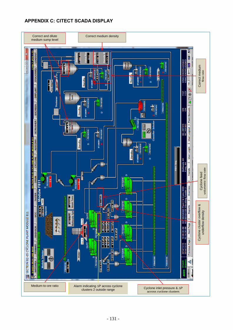
- 131 -

APPENDIX C: CITECT SCADA DISPLAY

Medium-to-ore ratio

Correct medium density

Cyclone inlet pressure & P across cyclone clusters

Cyclo

ne c

luste

r overf

low

&

underf

low

density

Alarm indicating P across cyclone clusters 2 outside range

Correct and dilute medium sump level

Cyclo

ne f

eed

volu

metr

ic f

low

rate

Corr

ect m

ediu

m

flo

w r

ate

Optimization of Dense Medium Cyclone Plant for the...

Documents

Transcript of Optimization of Dense Medium Cyclone Plant for the...