Optimization of AUVs propulsion system for underwater...

Optimization of AUVs propulsion system forunderwater infrastructures monitoring

MOQESM’16 - Sea Tech Week

Pablo Vega

PhD student atInstitut de Recherche Dupuy de Lome

CNRS FRE 3744PTR4 : Energie et Systemes - ENIB

Supervisor: O. Chocron Director: M. Benbouzid

Brest, 12thOctober 2016

Outline

1 Motivation

2 Our approach

3 AUV Model (solid and Hydrodynamics)

4 Control (model based)

5 Dynamic reconfiguration

6 Conclusions and perspectives

[email protected] 1 / 19 12/10/2016

mailto:[email protected]

Motivation

• AUV can be trusted to carry out complex missions• However, AUV development has not yet reached its full potential→ their capabilities can be still greatly improved.

• One of these characteristic is maneuverability, a key factor to achievefull autonomy.

• An enhanced maneuverability along with the possibilities offered bycurrent control methods and sensor technology could increase greatlythe complexity and reliability of AUV missions

Fig. 1. Marine turbine. EDFFig. 2. A9-EAUV ECA group



Our approach

• To give AUVs the capability to reconfigure their propulsion.• Adapt the propulsive topology and control parameters to the task

dynamically.• Use of vectorial thruster to achieve propulsion reconfiguration.• Use of model-based controller to cancel out nonlinearities.• A task-based design optimized propulsion topology and controller

increases maneuverability, leading to enhanced AUV autonomy.

Fig. 3. RMCT prototype. IRDL

Robot in-verse model

PID

Referencetrajectory

+

Robot State

Computed torque control

Fig. 4. Model based controller



Our approachSteps to follow

In order to implement our propulsion optimization approach we need todevelop the following elements:

• A dynamic model (solid andhydro) of an AUV. Based onprototype developed in IRDL: theRSM robot

• A control method allowing us tofollow a task trajectory.

• An optimization method in orderto find an optimal propulsiveconfiguration (topology andcontrol parameters) for a givenmission.

RSM robot (IRDL-ENIB) in Ifremer bassin



AUV modelKinematics

The vectors describing the movement of the AUV in 6 DOF are:

Position and orientation in R0

η =[η1η2

]η1 =

[xyz

]η2 =

[φθψ

]

Linear and angular velocity in Rb

ν =[ν1ν2

]ν1 =

[uvw

]ν2 =

[pqr

]

Efforts in Rb

τ =[τ1τ2

]τ1 =

[XYZ

]τ2 =

[KMN

]O

x y

z

Ob

xbSurge

ybSway

Pitch

zb Heave

Yaw

Roll

η1

Coordinate frames describing the AUV



AUV modelDynamics

The equation describing the underwater robot solid and hydro dynamics isthe following (Fossen):

Mν + Cν + Dν + G = τ = B up

with• M = MRB + MA, mass and inertia matrices• C = CRB + CA, coupling matrices• D = Damping matrix• G = Gravity and buoyancy• B = Thruster configuration matrix• up = Thrusters forces (thrust)



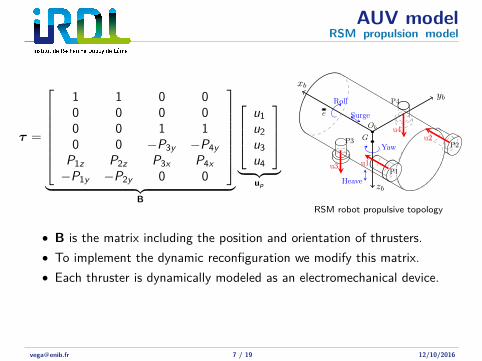
AUV modelRSM propulsion model

τ =

1 1 0 00 0 0 00 0 1 10 0 −P3y −P4y

P1z P2z P3x P4x−P1y −P2y 0 0

︸︷︷︸

B

u1u2u3u4

︸︷︷︸

up

Ob

G

e

xb

yb

zb

Roll

Surge

Heave

Yaw

u1P1

u2P2

u3

P3

u4

P4

RSM robot propulsive topology

• B is the matrix including the position and orientation of thrusters.• To implement the dynamic reconfiguration we modify this matrix.• Each thruster is dynamically modeled as an electromechanical device.



Control methodComputed torque

Principle• The idea is to algebraically transform nonlinear systems into (fully or partly)

linear ones in order to apply linear control methods.

• It creates a control input able to cancel out the nonlinear effects (inertia,coupling, drag, gravitational forces and buoyancy)

ηed Λ

ddt

J−1

Ro −→ Rb

T−1

re −→ Ob

+ ekin +

νad

+ ˙ηed

Kp Eq.3.5 Σedyn τa

ddt

+νad+

νad

ηe

−

ν−ν

Feedforward

Feedforward

Kinematic Control

Dynamic control



Control methodComputed torque

Two control laws in cascade:Kinematic law: Velocity

• derived from the robot inverse kinematic model.• generates the velocity reference to follow the desired trajectory.

νad = T−1 {J−1 [ηed + Λ ekin]}

with T a velocity transport matrix (rigid body kinematics)

Dynamic law: Acceleration• derived from the robot complete dynamic model.• generates the control input necessary to follow the reference velocity.

τa = M[νad + Kpedyn] + C(ν)ν + D(ν)ν + G



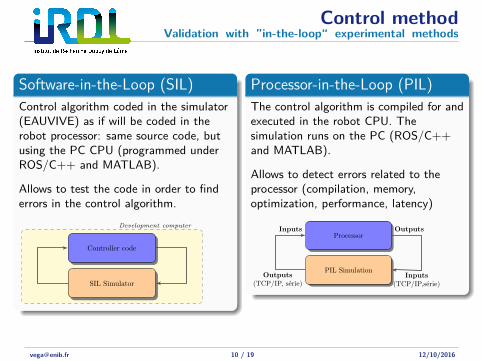
Control methodValidation with ”in-the-loop“ experimental methods

Software-in-the-Loop (SIL)Control algorithm coded in the simulator(EAUVIVE) as if will be coded in therobot processor: same source code, butusing the PC CPU (programmed underROS/C++ and MATLAB).

Allows to test the code in order to finderrors in the control algorithm.

Development computer

Controller code

SIL Simulator

Processor-in-the-Loop (PIL)The control algorithm is compiled for andexecuted in the robot CPU. Thesimulation runs on the PC (ROS/C++and MATLAB).

Allows to detect errors related to theprocessor (compilation, memory,optimization, performance, latency)

Processor

PIL SimulationInputs

(TCP/IP,serie)

Inputs Outputs

Outputs(TCP/IP, serie)

[email protected] 10 / 19 12/10/2016


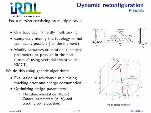
Dynamic reconfigurationPrinciple

For a mission consisting on multiple tasks:

• One topology ⇒ hardly multitasking• Completely modify the topology ⇒ not

technically possible (for the moment)• Modify actuators orientation + control

parameters ⇒ possible in the nearfuture X(using vectorial thrusters likeRMCT)

We do this using genetic algorithms:• Evaluation of solutions : minimizing

tracking error and energy consumption• Optimizing design parameters:

- Thrusters orientation (θi , ψi )- Control parameters (Λ, Kp and

tracking point position)

[ XYZMNK

]︸︷︷︸

τa

=

[ . . . cθi cψi . . .. . . cθi sψi . . .. . . −sθi . . .. . . −sθi Piy − cθi sψi Piz . . .. . . cθi cψi Piz + sθi Pix . . .. . . cθi sψi Pix − cθi cψi Piy . . .

]︸︷︷︸

B

...

ui...

︸︷︷︸

up

01

23

4

0

1

2

1

1.5

2

2.5

Seabed scan

Divingtoward turbine

Turbineinspection

Turbine

xy

z

Inspection mission

[email protected] 11 / 19 12/10/2016


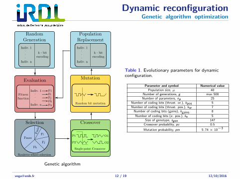
Dynamic reconfigurationGenetic algorithm optimization

Random Generation

Evaluation

Selection Crossover

Mutation

Indiv. 1

.

.

.

Indiv. n

k - bitencoding

Indiv. 1

.

.

.

Indiv. n

Fitnessfunction

F1FiFjFkFn

Fmax

Fm

in

Fi

Fj

Fk

Roulette-wheel selection

P1

P2

O1

O2

Single-point Crossover

Random bit mutation

Population Replacement

Indiv. 1

.

.

.

Indiv. n

k - bitencoding

Genetic algorithm

Table 1. Evolutionary parameters for dynamicconfiguration.

Parameter and symbol Numerical valuePopulation size, µ 40

Number of generations, g max 500Number of parameters, np 25

Number of coding bits (thrust. or.), kpos 5Number of coding bits (thrust. pos.), kor 7

Number of coding bits (gains), kgains 8Number of coding bits (e. pos.), ke 5

Size of genotype, sgen 147Crossover probability, pc 0.5Mutation probability, pm 5.74 × 10−3

[email protected] 12 / 19 12/10/2016


Dynamic reconfigurationResults - Seabed scanning

0 50 100 150 200 250 300 350 400 450 5000

10

20

30

Generation

Fitness

Best FitnessAverage fitness

35.52

29

Fitness evolution

0 100 200 300 400 500−2

−1

0

1

Generation

Orient.

[rad]

θ2 ψ2

0.21 ≡ 12.03°

−0.83 ≡ −47.55°

0 100 200 300 400 500

−1

0

1

2

Generation

Orient.

[rad]

θ4 ψ4

−0.41 ≡ −23.5°

−0.31 ≡ −17.76°

0 100 200 300 400 500

−1

0

1

Generation

Orient.

[rad]

θ3 ψ3

0.18 ≡ 10.31°

−1.57 ≡ −90°

0 100 200 300 400 500

0

1

Generation

Orient.

[rad]

θ1 ψ1

−0.73 ≡ −41.83°

1.47 ≡ 84.22°

0.22

0.24

0.26

0.28

0.3

Position[m

]

Pex

0.29

Best propulsive configuration

Final Λ = 1Final Kp = 1.5

[email protected] 13 / 19 12/10/2016


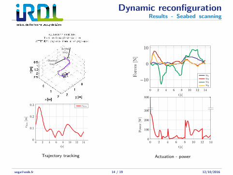
Dynamic reconfigurationResults - Seabed scanning

Desiredtraj.

Actualtraj.

0 2 4 6 8 10 12 140

0.1

0.2

0.3

t[s]

e kin

[m]

ekin

Trajectory tracking

0 2 4 6 8 10 12 14

−10

0

10

t[s]

Forces[N

]

u1u2u3u4

800

0 2 4 6 8 10 12 140

100

200

300

t[s]

Pow

er[W

]

Actuation - power

[email protected] 14 / 19 12/10/2016


Dynamic reconfigurationResults - Diving

0 50 100 150 200 250 300 350 400 450 5000

10

20

30

40

Generation

Fitness


36.4

29.32

Fitness evolution

0 100 200 300 400 500

−1

0

1

2

Generation

Orient.

[rad]

θ2 ψ2

1.17 ≡ 67.03°

−0.36 ≡ −20.62°

0 100 200 300 400 500

−1

0

1

Generation

Orient.

[rad]

θ4 ψ4

0

0

0 100 200 300 400 500

−1

0

1

Generation

Orient.

[rad]

θ3 ψ3

−1.35 ≡ −77.35°

0.23 ≡ 13.18°

0 100 200 300 400 500

−1

0

1

Generation

Orient.

[rad]

θ1 ψ1

−0.4 ≡ −23.5°

0.0 ≡ 0°

0.1

0.2

0.3

Position[m

]

Pex

0.3


Final Λ = 0.5Final Kp = 2.75

[email protected] 15 / 19 12/10/2016


Dynamic reconfigurationResults - Diving

Desiredtraj.

Actualtraj.

0 2 4 6 8 10

0.1

0.2

0.3

t[s]

e kin

[m]

ekin

Trajectory tracking

0 2 4 6 8 10

0

5

t[s]

Forces[N

]

u1u2u3u4

800

0 1 2 3 4 5 60

100

200

300

t[s]

Pow

er[W

]

Actuation - power

[email protected] 16 / 19 12/10/2016


Dynamic reconfigurationResults - Tomography

0 20 40 60 80 100 120 140 160 180 200 220 240 260 280 3000

10

20

30

Generation

Fitness


34.17

30.04

Fitness evolution

0 50 100 150 200 250 300−1

−0.5

0

0.5

Generation

Orient.

[rad]

θ2 ψ2

0

−0.51 ≡ −29.22°

0 50 100 150 200 250 300−1

0

1

Generation

Orient.

[rad]

θ4 ψ4

1.17 ≡ 67°

0.95 ≡ 54.43°

0 50 100 150 200 250 300

−1

0

1

Generation

Orient.

[rad]

θ3 ψ3

0.16 ≡ 9.17°

1.57 ≡ 90°

0 50 100 150 200 250 300

−1

0

1

Generation

Orient.

[rad]

θ1 ψ1

−0.82 ≡ −47°

1.52 ≡ 87°

0.1

0.2

Position[m

]

Pex

0.04


Final Λ = 0.25Final Kp = 9.25

[email protected] 17 / 19 12/10/2016


Dynamic reconfigurationResults - Tomography

Desiredtraj.

Actualtraj.

0

0.2

0.4

e kin

[m]

0 2 4 6 8 10

0

5 · 10−2

0.1

e ψ[rad

]

ekineψ

Trajectory tracking

0 2 4 6 8 10−40

−20

0

t[s]

Forces[N

]

u1u2u3u4

800

0 1 2 3 4 5 60

200

400

t[s]

Pow

er[W

]

Actuation - power

[email protected] 18 / 19 12/10/2016


Conclusions and perspectives

• Genetic algorithms allow to find an optimal propulsive configuration fora given task (in this work it includes thruster orientation, tracking pointposition and control gains).

• A robot using this technique could be optimally adapted to a missionincluding any number of tasks or sub-tasks. For instance seabedscanning could be split into a straight line and sharp turns.

• Current advances in reconfigurable thruster technology can make thistechnique applicable in the near future (such as RMCT work inIRDL-ENIB).

• The application of the genetic algorithm is susceptible of being improved(use of different GA techniques, improvement in the fitness functions...)

• Other control methods can be included as well in the optimization(robust, adaptive).

• Global optimization can be achieved adding other design parameters.

[email protected] 19 / 19 12/10/2016


Thank you foryour attention!AnyQuestions?

Optimization of AUVs propulsion system for underwater...

Documents

Transcript of Optimization of AUVs propulsion system for underwater...