OPTIMIZATION MODEL FOR BASE-LEVEL DELIVERY ROUTES AND

CREW SCHEDULING

THESIS

Young-ho Cha, Captain, ROKA

AFIT/GOR/ENS/05-02

DEPARTMENT OF THE AIR FORCE AIR UNIVERSITY

AIR FORCE INSTITUTE OF TECHNOLOGY

Wright-Patterson Air Force Base, Ohio

APPROVED FOR PUBLIC RELEASE; DISTRIBUTION UNLIMITED.

The views expressed in this thesis are those of the author and do not reflect the official policy or position of the United States Air Force, Department of Defense, or the United States Government.

AFIT/GOR/ENS/05-02

OPTIMIZATION MODEL FOR BASE-LEVEL DELIVERY ROUTES AND CREW SCHEDULING

THESIS

Presented to the Faculty

Department of Operational Sciences

Graduate School of Engineering and Management

Air Force Institute of Technology

Air University

Air Education and Training Command

In Partial Fulfillment of the Requirements for the

Degree of Master of Science in Operations Research

Young-ho Cha, BS

Captain, ROKA

March 2005

APPROVED FOR PUBLIC RELEASE; DISTRIBUTION UNLIMITED.

AFIT/GOR/ENS/05-02

OPTIMIZATION MODEL FOR BASE-LEVEL DELIVERY ROUTES AND CREW SCHEDULING

Young-ho Cha, BS Captain, ROKA

Approved: /signed/ ____________________________________

Lt Col. Jeffery D. Weir (Advisor) date

/signed/ ____________________________________

Maj. Victor D. Wiley (Reader) date

iv

AFIT/GOR/ENS/05-02

Abstract

In the US Air Force, a Logistic Readiness Squadron (LRS) provides material

management, distribution, and oversight of contingency operations. Dispatchers in the

LRS must quickly prepare schedules that meet the needs of their customers while dealing

with real-world constraints such as time windows, delivery priorities, and intermittent

recurring missions. Currently, LRS vehicle operation elements are faced with a shortage

of manpower and lack an efficient scheduling algorithm and tool. The purpose of this

research is to enhance the dispatchers’ capability to handle flexible situations and

produce “good” schedules within current manpower restrictions. In this research, a new

scheduling model and algorithm are provided as an approach to crew scheduling for a

base-level delivery system with a single depot. A Microsoft Excel® application, the

Daily Squadron Scheduler (DSS), was built to implement the algorithm. DSS combines

generated duties with the concept of a set covering problem. It utilizes a Linear

Programming pricing algorithm and Excel Solver as the primary engine to solve the

problem. Reduced costs and shadow prices from sub problems are used to generate a set

of feasible duties from which an optimal solution to the LP relaxation can be found.

From these candidate duties the best IP solution is then found. The culmination of this

effort was the development of both a scheduling tool and an analysis tool to guide the

LRS dispatcher toward efficient current and future schedules.

v

Acknowledgments

All the thanks in the world go to my wonderful wife. She carried the load at

home allowing me to devote myself to AFIT. I will forever be in debt to her sacrifices.

I would like to express my sincere appreciation to my faculty advisor, Lt Col.

Jeffery D. Weir, and reader, Maj. Victor D. Wiley, for their guidance and support

throughout the course of this thesis effort. Their insight and experience was certainly

appreciated.

I am also indebted to my classmates who spent their valuable time explaining the

current military systems and the realities they have experienced so far. Special thanks go

to Earl M. Bednar and Cole W. Gulyas who checked my English writing and were always

available to answer my questions.

Young-ho Cha

vi

Table of Contents

Page Abstract............................................................................................................................. iv Acknowledgments ............................................................................................................. v List of Figures................................................................................................................. viii List of Tables .................................................................................................................... ix Chapter 1. Introduction.................................................................................................... 1

1.1 Background............................................................................................................... 1 1.2 Problem Statement .................................................................................................... 2 1.3 Thesis Overview ....................................................................................................... 4

Chapter 2. Literature Review .......................................................................................... 5

2.1 Chapter Overview ..................................................................................................... 5 2.2 Scheduling Theory .................................................................................................... 5 2.3 Scheduling Problem.................................................................................................. 6 2.4 Traveling Salesman and Vehicle Routing Problems ................................................ 7 2.5 Crew Scheduling Problem (CSP).............................................................................. 9

2.5.1 Set Partitioning Problem(SPP)........................................................................... 9 2.5.2 Set Covering Problem (SCP) ........................................................................... 11

2.6 Integration of Vehicle Routing and Crew Scheduling............................................ 12 2.7 Programming Languages ........................................................................................ 14 2.8 Scheduling in the 48th LRS Environment .............................................................. 16 2.9 Implementation issue .............................................................................................. 19 2.10 Excel Solver .......................................................................................................... 20

2.10.1 Reduced Cost ................................................................................................. 21 2.10.2 Shadow Price ................................................................................................. 23

2.11 Heuristic (Simulated Annealing) .......................................................................... 24 2.12 Summary ............................................................................................................... 27

Chapter 3. Methodology................................................................................................. 28

3.1 Chapter Overview ................................................................................................... 28 3.2 Assumptions............................................................................................................ 28 3.3 Scheduling Goals and Objectives ........................................................................... 29 3.4 Scheduling Model and Problem Characteristics ..................................................... 30 3.5 Receive the daily recurring jobs and intermittent recurring jobs............................ 31

3.5.1 Daily recurring jobs ......................................................................................... 32 3.5.2 Intermittent recurring jobs ............................................................................... 33

3.6 Prioritize the jobs .................................................................................................... 34 3.7 Check the availability of drivers and their qualification......................................... 35 3.8 Preparatory processing (parameter set-up) ............................................................. 35 3.9 Generate Eligible Duties ......................................................................................... 40

vii

3.10 Generating Schedule ............................................................................................. 41 3.10.1 Pricing Approach ........................................................................................... 43 3.10.2 Heuristic (Simulated Annealing) ................................................................... 48 3.10.2.1 Representations of possible solutions ......................................................... 48 3.10.2.2 Generator of random changes in solutions.................................................. 49 3.10.2.3 Means of evaluating the problem functions................................................ 49 3.10.2.4 Annealing schedule..................................................................................... 50

3.11 Summary ............................................................................................................... 51 Chapter 4. Analysis and Results .................................................................................... 52

4.1 Chapter Overview ................................................................................................... 52 4.2 Physical Structures and the Performance of the Software ...................................... 52 4.3 Parameters Analysis................................................................................................ 54 4.4 Scheduling Scheme with Daily Recurring Jobs...................................................... 59

4.4.1 Military Schedule Comparison ........................................................................ 60 4.4.2 Civilian Schedule Comparison ........................................................................ 63

4.5 Notional Schedule................................................................................................... 66 4.6 Conclusion .............................................................................................................. 73

Chapter 5. Conclusions and Recommendations........................................................... 74

5.1 Specific Contributions ............................................................................................ 74 5.2 Recommendations for Future Work........................................................................ 75

Appendix A. Daily Recurring Responsibilities............................................................. 76 Bibliography .................................................................................................................... 77 Vita ................................................................................................................................... 79

viii

List of Figures

Page Figure 1-1 LRS Organizational Structure ........................................................................... 1 Figure 2-1 GVRP hierarchical classification scheme (Carlton, 1995) ............................... 8 Figure 2-2 Mapping a CSP solution to the SPP (Combs, 2002)....................................... 10 Figure 2-3 Conceptual map of 48th LRS........................................................................... 16 Figure 2-4 Concept of Zone and Sites .............................................................................. 17 Figure 2-5 VOE Scheduling Input Sources ...................................................................... 19 Figure 2-6 Tree with System of Algorithms (Muller-Merbach, 1981:6-8) ...................... 25 Figure 2-7 Structure of Simulated Annealing Algorithm ................................................. 26 Figure 3-1 LRS crew scheduling structure ....................................................................... 29 Figure 3-2 Daily recurring jobs......................................................................................... 32 Figure 3-3 Input Customer data (intermittent legs) .......................................................... 34 Figure 3-4 Parameter setting procedure screenshot .......................................................... 36 Figure 3-5 Example of One Shift Timeline (uncompleted) .............................................. 37 Figure 3-6 Example Duty.................................................................................................. 39 Figure 3-7 Example of 48th LRS’s Daily Published Operation Schedule......................... 41 Figure 3-8 Sample parameters .......................................................................................... 42 Figure 3-9 SCP & A-Matrix ............................................................................................. 42 Figure 3-10 Pricing Algorithm.......................................................................................... 45 Figure 3-11 Construction of an optimal solution.............................................................. 47 Figure 3-12 Avoiding Overlapped Legs ........................................................................... 47 Figure 3-13 Representation of possible solution .............................................................. 49 Figure 4-1 Start Up Menu ................................................................................................. 53 Figure 4-2 Shift vs. AvgDrivers........................................................................................ 56 Figure 4-3 Mealbreak vs. AvgDrivers .............................................................................. 57 Figure 4-4 Minsit vs. AvgDrivers..................................................................................... 57 Figure 4-5 Maxsit vs. AvgDrivers .................................................................................... 58 Figure 4-6 Maxworkload vs. AvgDrivers......................................................................... 58 Figure 4-7 Combination of Parameters for Military Schedule (1) & (2) .......................... 61 Figure 4-8 LRS Current Military Schedule ...................................................................... 62 Figure 4-9 DSS Military Schedule (1) .............................................................................. 62 Figure 4-10 Combination of Parameters for Civilian Schedule (1) & (2) ........................ 64 Figure 4-11 LRS Current Civilian Schedule..................................................................... 65 Figure 4-12 DSS Civilian Schedule (1) ............................................................................ 65 Figure 4-13 DSS Notional Run Results (62 Legs)............................................................ 67 Figure 4-14 DSS Notional Run Results (93 Legs)............................................................ 68 Figure 4-15 DSS Notional Run Results (124 Legs).......................................................... 69 Figure 4-16 DSS Notional Run (62 Legs) ........................................................................ 70 Figure 4-17 DSS Notional Run (93 Legs) ........................................................................ 71 Figure 4-18 DSS Notional Run (124 Legs) ...................................................................... 72

ix

List of Tables

Page Table 1-1 Personnel Status in LRS ..................................................................................... 3 Table 2-1 Minimum Daily Runs (delivery schedule) ....................................................... 18 Table 3-1 Category of Leg................................................................................................ 31 Table 4-1 Factors and Levels ............................................................................................ 55 Table 4-2 Current LRS Schedule Summary ..................................................................... 59 Table 4-3 DSS Results Summary (Military)..................................................................... 60 Table 4-4 DSS Results Summary (Civilian)..................................................................... 63 Table 4-5 Notional Run Set Up & Results........................................................................ 66

1

OPTIMIZATION MODEL FOR BASE-LEVEL

DELIVERY ROUTES AND CREW SCHEDULING

Chapter 1. Introduction

1.1 Background

The 48th Fighter Wing (FW) Royal Air Force (RAF) Lakenheath, England is

England’s largest U.S. Air Force-operated fighter base. It is located in the northeastern

part of London. The 48th Logistic Readiness Squadron (LRS) is part of the 48th Mission

Support Group (MSG), and provides materiel management, distribution, and support for

contingency operations of the 48th FW, United States Air Forces in Europe (USAFE), US

European Command (USEUCOM), and North Atlantic Treaty Organization (NATO)

commitments. It manages and operates a large fleet of vehicles, receives, stores, inspects

and delivers supplies; delivers petroleum; and directs the wing's deployment and plans

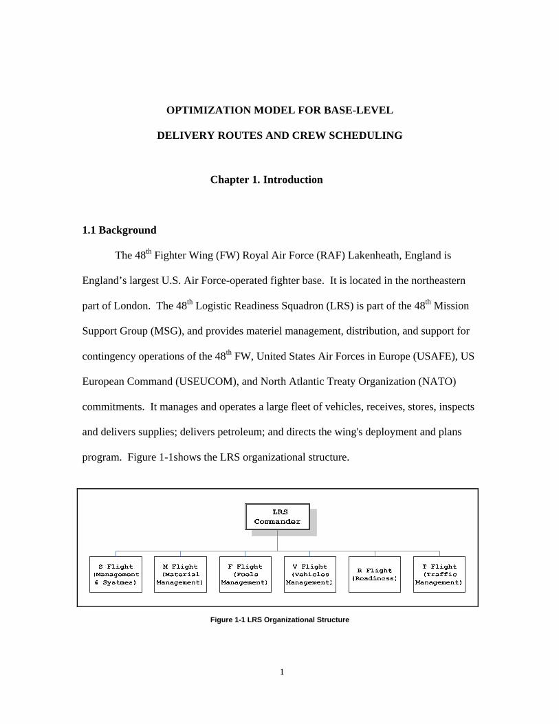
program. Figure 1-1shows the LRS organizational structure.

Figure 1-1 LRS Organizational Structure

2

This thesis is in response to the LRS’s request for support. This research focuses

on the V Flight. The V Flight is composed of Vehicle Operations and Vehicle

Maintenance. Vehicle Operations (VO) include delivery of property to customers across

the installation and to possibly geographically separated units using finite resources such

as drivers, vehicles, property, and time. The Vehicle Operations Element provides

efficient and economical 24-hour- a-day and 7- day- a- week ground traffic support for

the wing’s peace and wartime rapid deployment mission. This group has five primary

responsibilities: (1) pickup and delivery to include Redball deliveries (Redball deliveries

are unscheduled and urgent); (2) cargo and passenger movement for all wing

deployments; (3) flight line shuttle bus; (4) aircrew shuttle service for all three fighter

squadrons (492nd,493rd, and 494th); (5) Distinguished Visitor(DV) support, taxi and

wrecker service. The Vehicle Operations Element’s two major priorities are aircrew

shuttle and pickup and delivery.

1.2 Problem Statement

The LRS would like to optimize their schedule to support missions, based on their

resources. Resources limitations originally determined included number of drivers,

customer service time and numbers of vehicles. Fortunately, the LRS now operates a

sufficient number of vehicles and, during the course of conducting this research, the

vehicle constraints were discarded. The critical resource limitation is crew numbers. The

V Flight commander said, “The Pick Up and Delivery workload makes up 42% of the

total workload. Our Flight has the right number of personnel just not the right mix of

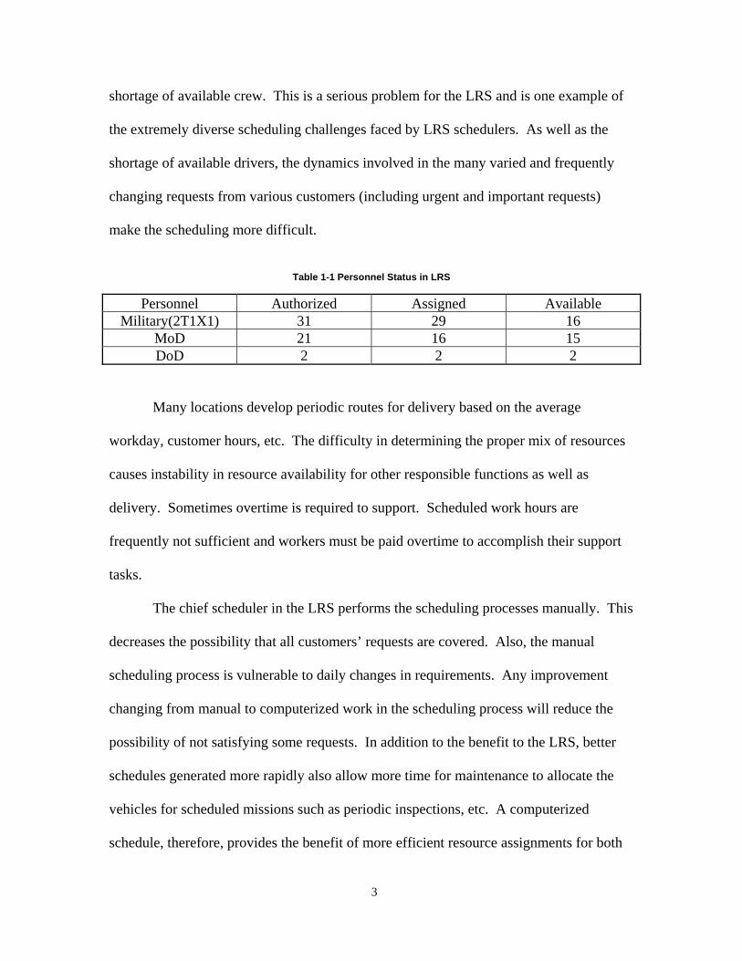
personnel.” Table 1-1explains the current LRS’s crew number level and highlights the

3

shortage of available crew. This is a serious problem for the LRS and is one example of

the extremely diverse scheduling challenges faced by LRS schedulers. As well as the

shortage of available drivers, the dynamics involved in the many varied and frequently

changing requests from various customers (including urgent and important requests)

make the scheduling more difficult.

Table 1-1 Personnel Status in LRS

Personnel Authorized Assigned Available Military(2T1X1) 31 29 16

MoD 21 16 15 DoD 2 2 2

Many locations develop periodic routes for delivery based on the average

workday, customer hours, etc. The difficulty in determining the proper mix of resources

causes instability in resource availability for other responsible functions as well as

delivery. Sometimes overtime is required to support. Scheduled work hours are

frequently not sufficient and workers must be paid overtime to accomplish their support

tasks.

The chief scheduler in the LRS performs the scheduling processes manually. This

decreases the possibility that all customers’ requests are covered. Also, the manual

scheduling process is vulnerable to daily changes in requirements. Any improvement

changing from manual to computerized work in the scheduling process will reduce the

possibility of not satisfying some requests. In addition to the benefit to the LRS, better

schedules generated more rapidly also allow more time for maintenance to allocate the

vehicles for scheduled missions such as periodic inspections, etc. A computerized

schedule, therefore, provides the benefit of more efficient resource assignments for both

4

operators and vehicles. Any tool that can assist scheduling and rescheduling will

decrease the amount of time spent on these processes, increase the efficiency of the

utilization of resources and also prevent overtasking of individuals.

1.3 Thesis Overview

The scope of this thesis is limited to the planning and generating of a daily

operator’s schedule, which consists of daily recurring runs and intermittent recurring runs,

while maximizing resource usage and maintaining a balanced workload among operators.

The model developed in this research also provides a re-scheduling ability to maximize

customer satisfaction and maintaining quality of service. This thesis contains four themes.

Chapter 2 provides the general information about the scheduling problem and specific

information about the scheduling problem at the 48th LRS. Chapter 3 outlines the

development of the scheduling model and a heuristic used to solve the scheduling

problems of the 48th LRS. In Chapter 4, model results are analyzed. Finally, Chapter 5

gives the summary of the research, contributions and recommendations for future

research.

5

Chapter 2. Literature Review

2.1 Chapter Overview

This chapter covers the concepts of scheduling, the topics related to vehicle

routing and crew scheduling theory, and using software-based visual interactive modeling

to generate schedules. In addition, the chapter also provides the background of the

scheduling environment at the 48th LRS.

2.2 Scheduling Theory

This section introduces concepts from scheduling theory. Scheduling concerns

the allocation of limited resources to tasks over time. It is a decision making process that

has as a goal the optimization of one or more objectives (Pinedo, 2002:1). Scheduling is

a decision-making process that exists in almost all operational environments. A

manufacturing facility has to manage the flow of its resources; the arrival of raw material,

worker shifts, and the departure of finished products. The scheduling function also faces

a variety of different problems in a service organization. One such problem might be

dealing with the reservation of resources, e.g., the assignment of aircraft to a future

mission even though they are not currently initialized (Pinedo, 2002:6).

The resources and tasks in an organization can take many forms. The resources

may be machines in a workshop, runways at an airport, crews at a construction site, a

processing unit in a computer environment, and so on. The tasks may be operations in a

production process, take offs and landings at an airport, stages in a construction project,

6

executions of computer programs and so on. The objectives can also take many forms.

One objective may be the minimization of the completion time of the last task commonly

referred to a ‘makespan’, another may be the minimization of the number of tasks

completed after their respective due dates (Pinedo, 2002:1).

2.3 Scheduling Problem

The scheduling problem has attracted much interest from both academia and the

operational world (Evren, 1999). Many theoretical research topics are directed towards

simple machine scheduling problems. In the operational world, scheduling environments

are much more complex and cannot be directly extrapolated to some simple theoretical

machine-scheduling model. Pinedo outlines some of the most common problems

encountered in scheduling. Empirically, the problems that are relevant to resource

scheduling environments are summarized by Pinedo as:

Theoretical models usually assume that there are n jobs to be scheduled and that after scheduling these n jobs, the problem is solved. In reality, new jobs are added or current jobs are re-scheduled continuously. The dynamic nature of resource scheduling in services may require that slack times be built into the schedule in expectation of the unexpected. Theoretical models usually do not emphasize the resequencing problem. In practice, the following problem often occurs: There exists a schedule, which was determined earlier based on certain assumptions, and an (unexpected) random event occurs that requires either major or minor modifications in the existing schedule. The rescheduling process, which is sometimes referred to as reactive scheduling, may have to satisfy certain constraints. For example, one may wish to keep the changes in the existing schedule at a minimum even if an optimal schedule cannot be achieved this way. This implies that it is advantageous to construct schedules that are in a sense robust. That is, resequencing brings about only minor changes in the schedule. The opposite of robust is often referred to as brittle.

7

Real world scheduling environments are often more complicated than the ones considered in general scheduling theory. In the mathematical models, the weights (priorities) of the jobs are assumed to be fixed (i.e., they do not change over time). In practice, the weight of a job often fluctuates over time due to changing priorities in the organization or a number of other factors.

Mathematical models often do not take preferences into account. A scheduler may favor some assignment for some reasons that cannot be incorporated into the model. Most theoretical research has focused on models with a single objective. Most real world problems exhibit multi-criteria and multi-objective characteristics, which sometimes are in conflict with each other (Pinedo, 2002:392).

Pinedo states that scheduling is the decision-making process that exists in most

manufacturing and production systems as well as in most information-processing

environments (Pinedo, 2002:1). Scheduling in these settings allocates resources to

different tasks over a period of time.

2.4 Traveling Salesman and Vehicle Routing Problems

The traveling salesman (agent) problem (TSP) and the vehicle routing problem

(VRP) are two classic problems of operations research. The two problems are closely

related. In the TSP, a single salesman must visit a set of customers or cities, visiting

every customer exactly once, and return home. A cost is associated with travel between

two customers. Thus, the objective is to find the lowest cost tour. A tour is an ordered

list of customers representing the salesman’s cycle through the set of customers. For the

single salesman TSP, it is assumed that the salesman has unconstrained ability to pay the

cost of the tour. Extensions to this basic problem include the following: multiple

8

traveling salesmen and time windows for each customer. The literature contains many

examples of different varieties of these problems. Lawler et al (1985) discuss the TSP

and its variants in depth. The TSP forms the basis for the vehicle routing problem (VRP).

As opposed to the model of a salesman, a vehicle servicing a set of customers is

subject to side constraints. Servicing a customer could involve either picking up or

delivering a product, but not both. The side constraints can be the service capacity of the

model vehicle, vehicle range, customer demands, or customer service times. Each tour

must start and end at the same depot. The objective is to find a set of minimal cost tours

that service all customers without violating any side constraints. Like the TSP, there are

several extensions to the VRP. Extensions to this basic problem include Capacitated

Vehicle Routing Problem (CVRP), Multiple Depot VRP (MDVRP), and VRP with Time

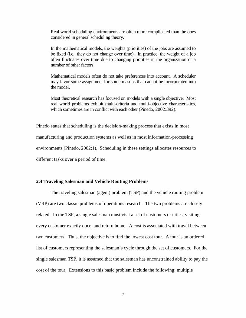
Window (VRPTW). Carlton (1995) creates a hierarchical classification scheme for the

General VRP (GVRP). Figure 2-1 demonstrates the tier for the TSP, VRP, and pickup

and delivery problems (PDP). In a VRP, the vehicles perform either delivery or pickup

operations exclusively. A PDP extends the VRP so that vehicles can make one or more

pickups from customers along the route for delivery to other customers.

Figure 2-1 GVRP hierarchical classification scheme (Carlton, 1995)

9

2.5 Crew Scheduling Problem (CSP)

The CSP concerns assigning crew duties to legs (or trips) with the objective of

minimizing the crew cost. This CSP can be expressed in formulaic fashion as follows.

Let’s assume n legs L1,… ,Ln have to be covered by a set of crews. Each leg Lj requires

uninterrupted driving from a starting point at a given starting time sj to an ending point at

a given ending time ej ≥ sj, and has a weight wj ≥ 0 (usually equal to ej - sj). In addition, a

working-time limit is specified. An ordered leg pair (Li , Lj) is called infeasible if the

same crew cannot cover Lj immediately after Li , for example because ej > sj ; otherwise,

it is called feasible. Todd E. Combs discusses the CSP and its variants in perspective of

airline crew scheduling problem in his dissertation paper (2002:25). Freling et al deals an

integrated approach to vehicle and crew scheduling for an urban mass transit system with

a single depot (Freling and others, 2003:63).

2.5.1 Set Partitioning Problem (SPP)

Traditionally a crew scheduling problem is modeled as the set partitioning

problem. When every leg must be served by exactly one duty, the problem takes on the

set partitioning format. Commonly cited problems having this structure include the crew-

scheduling problem in which every flight of an airline must be scheduled by exactly one

cockpit crew. The binary integer programming formulation for such a problem is given

below:

1min

: ,{0,1} 1,...,

n

j jj

m

j

c x

subject to Ax ex for j n

=

=∈ =

∑ (1)

10

Where em is a vector of m ones, and n is the number of duties that we consider. Each row

of the m × n A matrix represents a leg or segment, while each column represents a driver

duty with cost cj for using it. The xj are zero-one variables associated with each duty, i.e.,

xj=1 if duty j is executed. The A matrix is generated one column at a time, with aij=1 if

leg i is covered by duty j, 0 otherwise. In a set partitioning problem, each member of a

given set, S1, must be assigned to or partitioned by a member of a second set, S2. For the

air crew scheduling problem, each member of the set of flights must be assigned to a

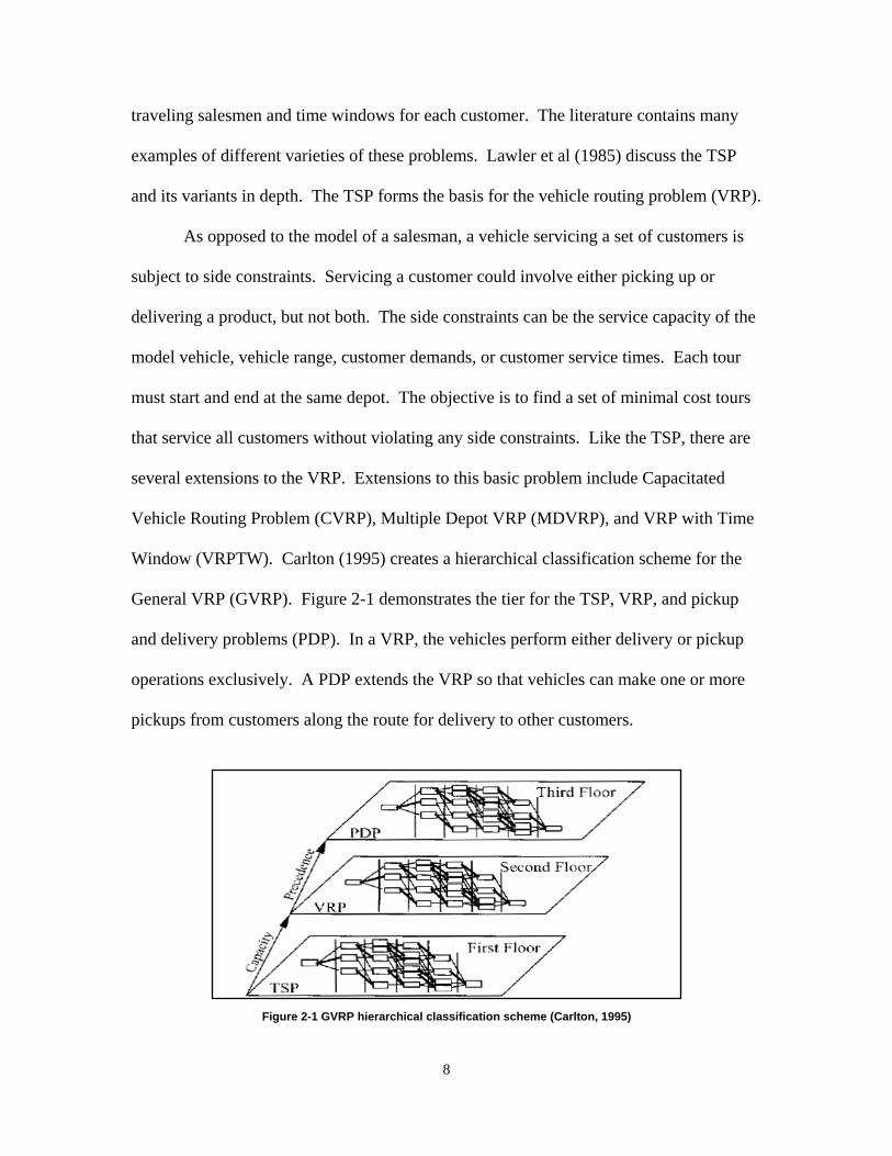
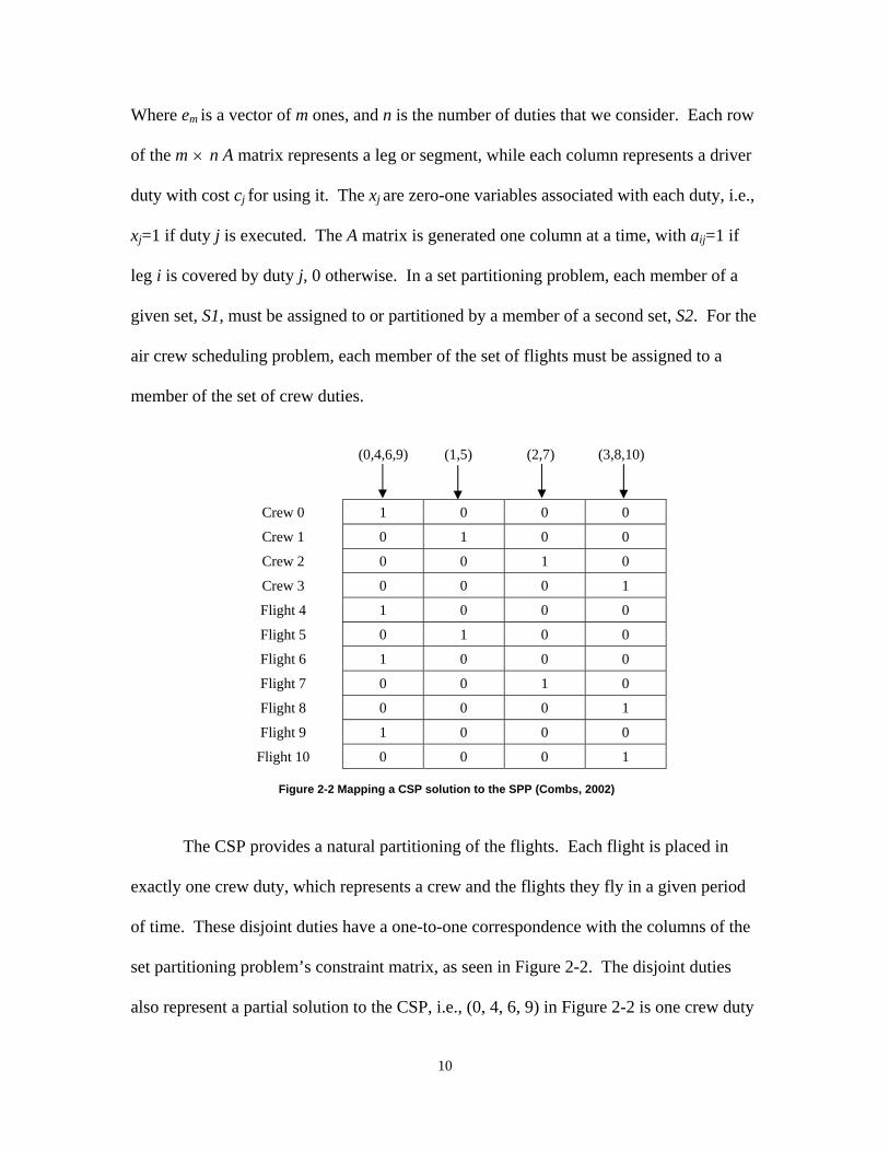
member of the set of crew duties.

(0,4,6,9) (1,5) (2,7) (3,8,10)

Crew 0 1 0 0 0

Crew 1 0 1 0 0

Crew 2 0 0 1 0

Crew 3 0 0 0 1

Flight 4 1 0 0 0

Flight 5 0 1 0 0

Flight 6 1 0 0 0

Flight 7 0 0 1 0

Flight 8 0 0 0 1

Flight 9 1 0 0 0

Flight 10 0 0 0 1

Figure 2-2 Mapping a CSP solution to the SPP (Combs, 2002)

The CSP provides a natural partitioning of the flights. Each flight is placed in

exactly one crew duty, which represents a crew and the flights they fly in a given period

of time. These disjoint duties have a one-to-one correspondence with the columns of the

set partitioning problem’s constraint matrix, as seen in Figure 2-2. The disjoint duties

also represent a partial solution to the CSP, i.e., (0, 4, 6, 9) in Figure 2-2 is one crew duty

11

within the solution set of crew duties. Todd E. Combs also discusses the SPP from a

historical perspective (2002:28).

2.5.2 Set Covering Problem (SCP)

In this section a mathematical formulation for the CSP is given. In the set

covering formulation of the CSP, the objective is to select a minimum cost set of feasible

duties such that each task is included in at least one of these duties. This is the following

0-1 linear program:

1

min

: ,{0,1} 1,...,

n

j jj

m

j

c x

subject to Ax ex for j n

=

≥

∈ =

∑ (2)

As the reader could see from the above formulation, the equations in SPP are

replaced by inequalities. The advantage of working with this formulation instead of a set

partitioning one is that it is easier to solve. After solving the set covering formulation,

the solution can be always changed into a set partitioning solution by deleting over-

covers of legs. In fact, this may be resolved by merely changing some of the selected

duties. Instead of being the driver, the person who is assigned to such a duty will stay at

LRS for the unscheduled job. Note that such changes affect neither the feasibility nor the

cost of the duties involved.

It is well known that the SCP is NP-complete (Beasley, 1990:151) and a number

of optimal algorithms have been proposed in the literature for the exact solution of SCP

(see Balas and Ho 1980, Beasley 1987, Fisher and Kedia 1990, Beasley and Jörnsten

12

1992, Nobili and Sassano 1992, and Balas and Carrera 1996). These exact algorithms

can solve instances with up to a few hundred rows and a few thousand columns. When

larger scale SCP instances are tackled, heuristic algorithms are needed. Classical greedy

algorithms are very fast in practice, but typically do not provide high quality solutions, as

reported in Balas and Ho (1980) and Balas and Carrera (1996). The most effective

heuristic approaches to SCP are those based on Lagrangian relaxation with sub gradient

optimization, following the seminal work by Balas and Ho (1980), and then the

improvements by Beasley (1990), Fisher and Kedia (1990), Balas and Carrera (1996),

and Ceria et al. (1995). Lorena and Lopes (1994) propose an analogous approach based

on surrogate relaxation. Wedelin (1995) proposes a general heuristic algorithm for

integer programs having a 0-1 constraint matrix; the algorithm is based on Lagrangian

relaxation with coordinate search, where a suitably-defined approximation term is

introduced. Recently, Beasley and Chu (1996) proposed an effective genetic algorithm.

2.6 Integration of Vehicle Routing and Crew Scheduling

Although in the early 1980s several researchers recognized the need to integrate

vehicle and crew scheduling for an urban mass transit system, most of the algorithms

published in the literature still follow the sequential approach in which vehicles are

scheduled before, and independently of, crews. Algorithms incorporated into

commercially successful computer packages use this sequential approach as well, while

sometimes integration is dealt with at the user level. In the operations research literature,

only a few publications make a comparison/contrast between simultaneous and sequential

scheduling.

13

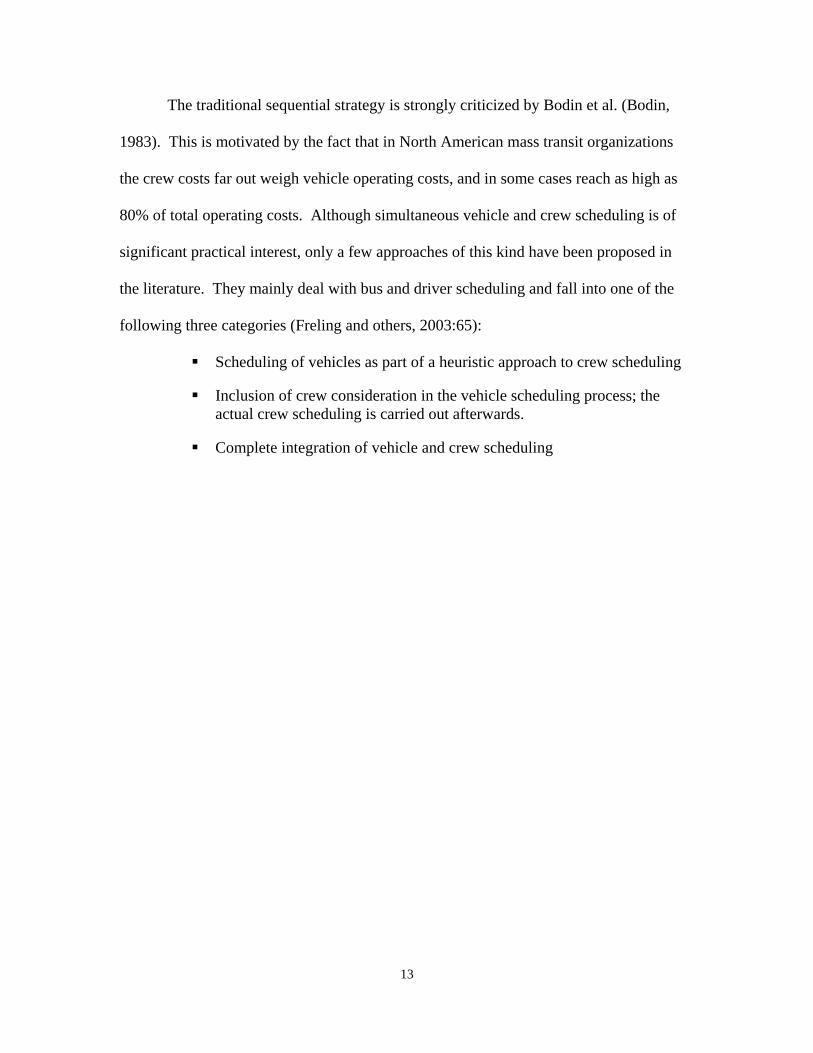
The traditional sequential strategy is strongly criticized by Bodin et al. (Bodin,

1983). This is motivated by the fact that in North American mass transit organizations

the crew costs far out weigh vehicle operating costs, and in some cases reach as high as

80% of total operating costs. Although simultaneous vehicle and crew scheduling is of

significant practical interest, only a few approaches of this kind have been proposed in

the literature. They mainly deal with bus and driver scheduling and fall into one of the

following three categories (Freling and others, 2003:65):

Scheduling of vehicles as part of a heuristic approach to crew scheduling Inclusion of crew consideration in the vehicle scheduling process; the

actual crew scheduling is carried out afterwards. Complete integration of vehicle and crew scheduling

14

2.7 Programming Languages

To implement any heuristics or rule-based algorithms, programming languages

must be considered. To select the right programming language, considerations of the

selection must be based on their availability as well as being easy to learn and use. The

majority of the desktop computers in the scheduling division use a version of the

Microsoft Windows operating system. “Since Microsoft also develops the MS Office

Suite on the foundation of Visual Basic engine, they can build enhancements and

attachment modules into the application to solve specific problems, and is assured a very

high probability of error free integration” (Nguyen, 2002:21).

MS office products such as Access, Word, and Excel have become the main word

processor, database and spreadsheet in the majority of offices and homes. The required

software is already present in the office documents because these come already pre-

installed with the computers when they are first purchased. 48th LRS scheduling division

used to generate and publish the schedules with MS Excel spreadsheet. Visual Basic is

used for these compelling reasons over Java and other object oriented programming

languages.

In VBA, the attributes of an object are called properties: e.g. the size and color of

an object. In addition, each property has a value associated with it. For example, a car

might be white and it may have four doors. In contrast, the things can be done to an

object are called methods: the drive method and the park method, for example. Methods

can take qualifiers, called arguments, which indicate how a method is carried out

(Albright, 2001:7).

15

Some of the most common objects in Excel are ranges, worksheets, charts and

workbooks. For example, consider the single-cell range B5. This range is considered a

Range object. It has a Value property: the value (either text or numeric) in the cell. A

Range object also has methods. For example, a range can be copied. The Copy method

takes the destination as its argument.

There is an object hierarchy in Microsoft Excel Objects. At the top of the

hierarchy is the Application object. This refers to Excel itself. One step down from

application is the Workbooks collection. One step down from Workbook is the

Worksheet objects and the other objects follow it (Albright, 2001:8-9).

16

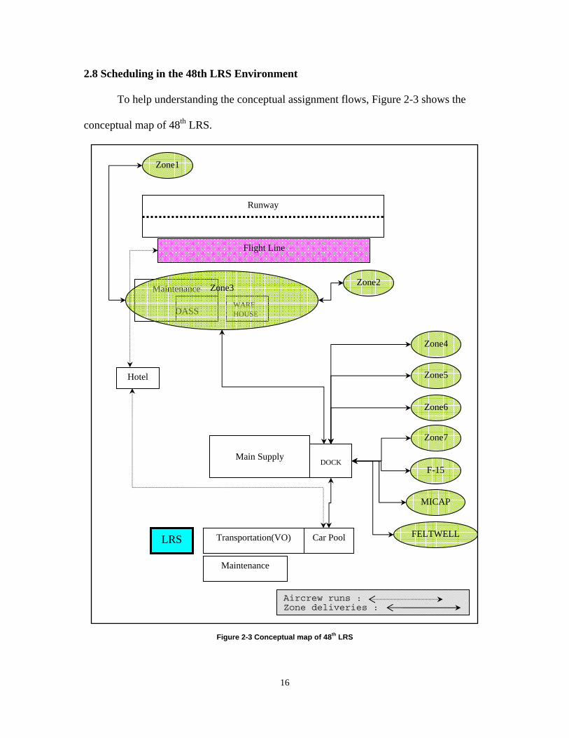
2.8 Scheduling in the 48th LRS Environment

To help understanding the conceptual assignment flows, Figure 2-3 shows the

conceptual map of 48th LRS.

Figure 2-3 Conceptual map of 48th LRS

Runway

Flight Line

Maintenance

DASS WARE HOUSE

Main Supply DOCK

Transportation(VO)

Maintenance

LRS

Hotel

Car Pool

Zone1

Zone2 Zone3

Zone4

Zone5

Zone6

F-15

MICAP

FELTWELL

Zone7

Aircrew runs :Zone deliveries :

17

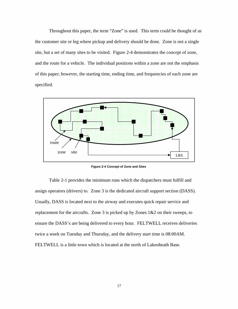
Throughout this paper, the term “Zone” is used. This term could be thought of as

the customer site or leg where pickup and delivery should be done. Zone is not a single

site, but a set of many sites to be visited. Figure 2-4 demonstrates the concept of zone,

and the route for a vehicle. The individual positions within a zone are not the emphasis

of this paper; however, the starting time, ending time, and frequencies of each zone are

specified.

Figure 2-4 Concept of Zone and Sites

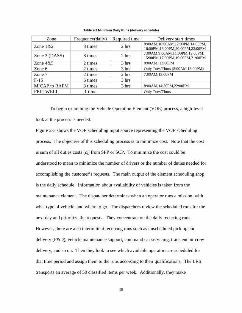
Table 2-1 provides the minimum runs which the dispatchers must fulfill and

assign operators (drivers) to. Zone 3 is the dedicated aircraft support section (DASS).

Usually, DASS is located next to the airway and executes quick repair service and

replacement for the aircrafts. Zone 3 is picked up by Zones 1&2 on their sweeps, to

ensure the DASS’s are being delivered to every hour. FELTWELL receives deliveries

twice a week on Tuesday and Thursday, and the delivery start time is 08:00AM.

FELTWELL is a little town which is located at the north of Lakenheath Base.

LRS zone site

route

18

Table 2-1 Minimum Daily Runs (delivery schedule)

Zone Frequency(daily) Required time Delivery start times Zone 1&2 8 times 2 hrs 8:00AM,10:00AM,12:00PM,14:00PM,

16:00PM,18:00PM,20:00PM,22:00PM

Zone 3 (DASS) 8 times 2 hrs 7:00AM,9:00AM,11:00PM,13:00PM, 15:00PM,17:00PM,19:00PM,21:00PM

Zone 4&5 2 times 3 hrs 8:00AM, 13:00PM Zone 6 2 times 3 hrs Only Tues/Thurs (8:00AM,13:00PM) Zone 7 2 times 2 hrs 7:00AM,13:00PM F-15 6 times 3 hrs MICAP to RAFM 3 times 3 hrs 8:00AM,14:30PM,22:00PM FELTWELL 1 time Only Tues/Thurs

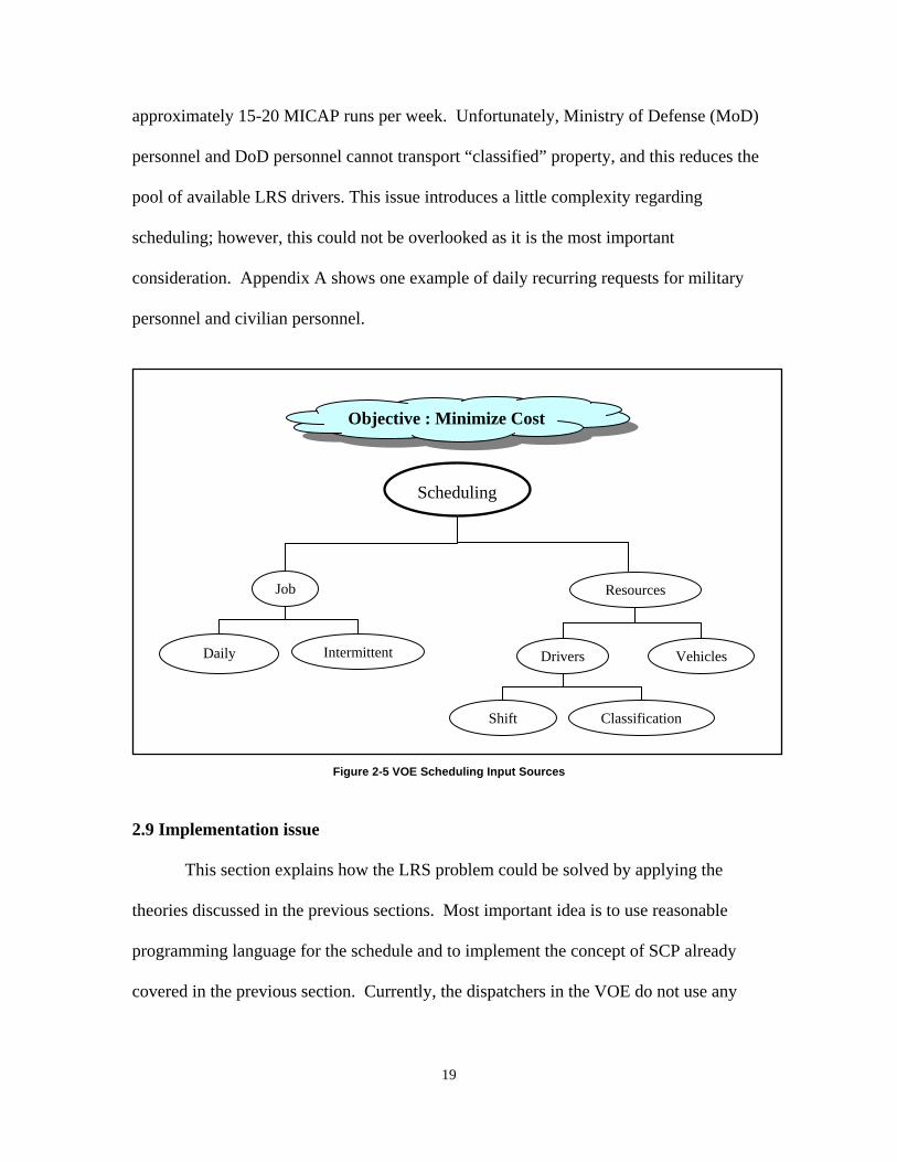
To begin examining the Vehicle Operation Element (VOE) process, a high-level

look at the process is needed.

Figure 2-5 shows the VOE scheduling input source representing the VOE scheduling

process. The objective of this scheduling process is to minimize cost. Note that the cost

is sum of all duties costs (cj) from SPP or SCP. To minimize the cost could be

understood to mean to minimize the number of drivers or the number of duties needed for

accomplishing the customer’s requests. The main output of the element scheduling shop

is the daily schedule. Information about availability of vehicles is taken from the

maintenance element. The dispatcher determines when an operator runs a mission, with

what type of vehicle, and where to go. The dispatchers review the scheduled runs for the

next day and prioritize the requests. They concentrate on the daily recurring runs.

However, there are also intermittent recurring runs such as unscheduled pick up and

delivery (P&D), vehicle maintenance support, command car servicing, transient air crew

delivery, and so on. Then they look to see which available operators are scheduled for

that time period and assign them to the runs according to their qualifications. The LRS

transports an average of 50 classified items per week. Additionally, they make

19

approximately 15-20 MICAP runs per week. Unfortunately, Ministry of Defense (MoD)

personnel and DoD personnel cannot transport “classified” property, and this reduces the

pool of available LRS drivers. This issue introduces a little complexity regarding

scheduling; however, this could not be overlooked as it is the most important

consideration. Appendix A shows one example of daily recurring requests for military

personnel and civilian personnel.

Figure 2-5 VOE Scheduling Input Sources

2.9 Implementation issue

This section explains how the LRS problem could be solved by applying the

theories discussed in the previous sections. Most important idea is to use reasonable

programming language for the schedule and to implement the concept of SCP already

covered in the previous section. Currently, the dispatchers in the VOE do not use any

Scheduling

Job

Drivers Vehicles

Resources

Daily Intermittent

Shift Classification

Objective : Minimize Cost

20

computer package tool or scheduling model. Depending on the manual approach to the

dynamic environment does not guarantee any efficient solution. Dispatchers may well be

able to make a feasible schedule, but there is no effective means to measure how their

schedule is good or to find more compatible schedules. A model based on VBA could

enhance their capability for making good schedules and provide the scheduler with a

more flexible plan to create a dynamic scheduling environment.

It is very reasonable to find some analogy between SCP and the LRS’s scheduling

environments to advance the research. Under current protocol, every leg (or trip) must be

covered exactly once at a scheduled time (SPP). When the ‘exactly once’ constraint is

relaxed, the problem is reduced to the SCP. If a schedule gets some over-cover legs, then

the extra legs which don’t need to be done could be reassigned to other assignments. In

some sense, the over-cover legs provide more flexibility to the scheduler. For instance, if

one driver were freed from responsibility for a leg, then he/she could be assigned to other

tasks (e.g. emergency delivery, washing vehicles, etc).

2.10 Excel Solver

Solver is part of a suite of commands sometimes called what-if analysis tools.

What-if analysis is a process of changing the values in cells to see how those changes

affect the outcome of formulas on the worksheet, for example, the user might vary the

interest rate that is used in an amortization table to determine the amount of the

payments. With Solver, the user can find an optimal value for a formula in one cell—

called the target cell— on a worksheet. A formula is a sequence of values, cell

references, names, functions, or mathematical operators in a cell that together produce a

21

new value. Solver works with a group of cells that are related, either directly or

indirectly, to the formula in the target cell. Solver adjusts the values in the changing

cells— called the adjustable cells— specified by the user to produce a user specified

result in the target cell formula (usually maximization or minimization). The user can

apply constraints which are the limitations placed on a Solver problem. The user can

apply constraints to adjustable cells, the target cell, or other cells that are directly or

indirectly related to the target cell to restrict the values Solver can use in the model. The

constraints can also refer to other cells that affect the target cell formula. Solver

determines the maximum or minimum value of one cell by changing other cells. For

example, the user can change the amount of a projected advertising budget and see the

affect on the projected profit amount.

The Microsoft Excel® Solver tool uses the Generalized Reduced Gradient (GRG2)

nonlinear optimization code developed by Leon Lasdon, University of Texas at Austin,

and Allan Warren, Cleveland State University. Integer problems use this method and the

branch-and-bound method, implemented by John Watson and Dan Fylstra, Frontline

Systems, Inc.

2.10.1 Reduced Cost

Consider the following linear programming problem:

0≥

=x

bAxcx

toSubjectMinimize

(3)

22

Where A is an m × n matrix with rank m. Suppose that we have a basic feasible solution

⎟⎟⎠

⎞⎜⎜⎝

⎛ −

0

1bB whose objective value z0 is given by

bBcbB

ccbB

c BNB1

11

00−

−−

=⎟⎟⎠

⎞⎜⎜⎝

⎛=⎟⎟

⎠

⎞⎜⎜⎝

⎛= ),(z0 (3.1)

Now let xB and xN denote the set of basic and nonbasic variables for the given basis.

Then feasibility requires that xB ≥ 0, xN ≥ 0, and that b = Ax = BxB + NxN.

Multiplying the last equation by B-1 and rearranging the terms, we get

∑

∑

∈

∈

−−

−−

−=

−=

−=

Rjjj

Rjjj

N

xyb

xaBbB

NxBbB

,say,)(

x B11

11

(3.2)

Where R is the current set of the indices of the nonbasic variables. Noting Equations

(3.2) and (3.1) and letting z denote the objective function value, we get

∑

∑∑

∈

∈∈

−−

−−=

+−=

+==

Rjjjj

Rjjj

RjjjB

NNBB

xcz

xcxaBbBc

xcxccx

)(z

)(

z

0

11 (3.3)

Where zj = cBB-1aj and yj=B-1aj for each nonbasic variable.

Using the foregoing transformations, the linear programming problem LP may be

rewritten as

23

0,,0

)(Subject to

)(Minimize 0

≥∈≥

=+

−−=

∑

∑

∈

∈

Bj

RjBjj

Rjjjj

xandRjx

bxxy

xczzz

(4)

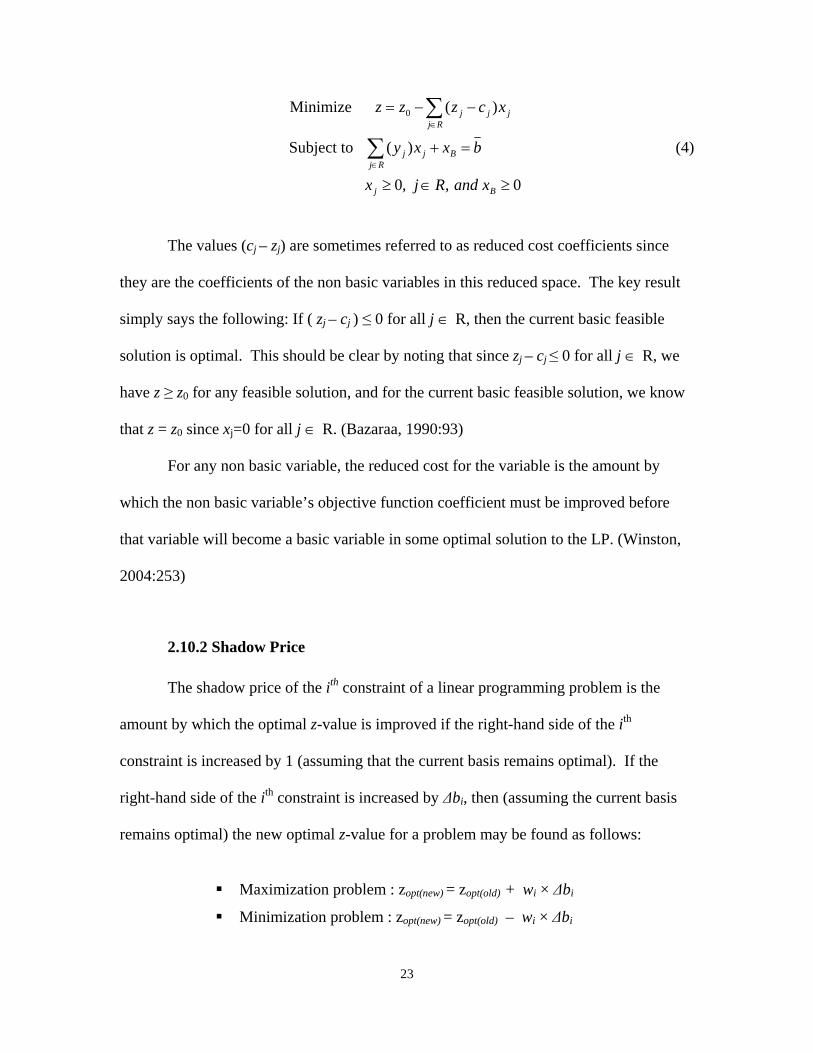
The values (cj – zj) are sometimes referred to as reduced cost coefficients since

they are the coefficients of the non basic variables in this reduced space. The key result

simply says the following: If ( zj – cj ) ≤ 0 for all j ∈ R, then the current basic feasible

solution is optimal. This should be clear by noting that since zj – cj ≤ 0 for all j ∈ R, we

have z ≥ z0 for any feasible solution, and for the current basic feasible solution, we know

that z = z0 since xj=0 for all j ∈ R. (Bazaraa, 1990:93)

For any non basic variable, the reduced cost for the variable is the amount by

which the non basic variable’s objective function coefficient must be improved before

that variable will become a basic variable in some optimal solution to the LP. (Winston,

2004:253)

2.10.2 Shadow Price

The shadow price of the ith constraint of a linear programming problem is the

amount by which the optimal z-value is improved if the right-hand side of the ith

constraint is increased by 1 (assuming that the current basis remains optimal). If the

right-hand side of the ith constraint is increased by ∆bi, then (assuming the current basis

remains optimal) the new optimal z-value for a problem may be found as follows:

Maximization problem : zopt(new) = zopt(old) + wi × ∆bi

Minimization problem : zopt(new) = zopt(old) – wi × ∆bi

24

Where, zopt(new) is new optimal z-value, zopt(old) = old optimal z-value, and wi is constraint

i’s shadow price (Winston, 2004:252).

For a maximization LP, the shadow price of the ith constraint is the value of the ith

dual variable in the optimal dual solution. For a minimization LP, the shadow price of

the ith constraint = – (ith dual variable in the optimal dual solution). A ≥ constraint will

have a nonpositive shadow price; a ≤ constraint will have a nonnegative shadow price;

and an equality constraint may have a positive, negative, or zero shadow price. (Winston,

2004:344)

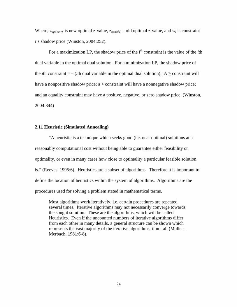
2.11 Heuristic (Simulated Annealing)

“A heuristic is a technique which seeks good (i.e. near optimal) solutions at a

reasonably computational cost without being able to guarantee either feasibility or

optimality, or even in many cases how close to optimality a particular feasible solution

is.” (Reeves, 1995:6). Heuristics are a subset of algorithms. Therefore it is important to

define the location of heuristics within the system of algorithms. Algorithms are the

procedures used for solving a problem stated in mathematical terms.

Most algorithms work iteratively, i.e. certain procedures are repeated several times. Iterative algorithms may not necessarily converge towards the sought solution. These are the algorithms, which will be called Heuristics. Even if the uncounted numbers of iterative algorithms differ from each other in many details, a general structure can be shown which represents the vast majority of the iterative algorithms, if not all (Muller-Merbach, 1981:6-8).

25

ApproximationAlgorithms

Path StructureAlgorithms

Tree StructureAlgorithms

FiniteAlgorithms

ConvergingAlgorithms

Algorithms withoutproven convergence

(Heuristics)

IterativeAlgorithms

DirectAlgorithms

Algorithms

Figure 2-6 Tree with System of Algorithms (Muller-Merbach, 1981:6-8)

In terms of computational complexity, the SCP belongs to the class NP-hard in

the strong sense. A polynomial-time algorithm does not exist for members of this class.

The number of possible solutions to the SCP grows exponentially as the number of duties

(or sets) increases. Throughout this research, the Simulated Annealing (SA) heuristic

will be implemented. Heuristic approaches provide no guarantee of optimality, although

most provide at least a feasible solution in a relatively short amount of time. Timeliness

of a solution is very important for our implementation, as LRS operations are typically

time-sensitive.

SA is a local search inspired by the process of annealing in physics (Kirkpatrick et

al., 1983). It is widely used to solve combinatorial optimization problems, especially to

avoid becoming trapped in local optima when using simpler local search methods (Aarts

et al., 1997). This is done as follows: an improving move is always accepted while a

worsening one is accepted according to a probability which depends on the amount of

deterioration in the evaluation function value. In other words, the less successful a move

26

is demonstrated to be, the less likely it is to be accepted. Formally a move is accepted

according to the following probability distribution, dependent on a virtual temperature T,

known as the Metropolis distribution:

⎪⎩

⎪⎨⎧ ≤

= −−

otherwise

)()'(if1)',,( ))()'((

Tsfsfaccept

e

sfsfssTp

Where s is the current solution, s’ is the neighbor solution and f(s) is the evaluation

function. The temperature parameter T, which controls the acceptance probability, is

allowed to vary over the course of the search process. Figure 2-7 shows its basic

structure.

Figure 2-7 Structure of Simulated Annealing Algorithm

27

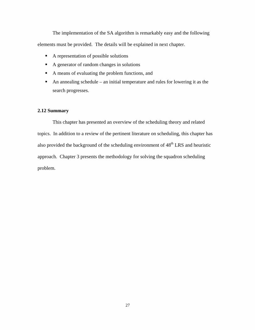
The implementation of the SA algorithm is remarkably easy and the following

elements must be provided. The details will be explained in next chapter.

A representation of possible solutions

A generator of random changes in solutions

A means of evaluating the problem functions, and

An annealing schedule – an initial temperature and rules for lowering it as the

search progresses.

2.12 Summary

This chapter has presented an overview of the scheduling theory and related

topics. In addition to a review of the pertinent literature on scheduling, this chapter has

also provided the background of the scheduling environment of 48th LRS and heuristic

approach. Chapter 3 presents the methodology for solving the squadron scheduling

problem.

28

Chapter 3. Methodology

3.1 Chapter Overview

This chapter describes the methodology to be employed in the thesis. This

chapter is partitioned into three distinct areas: assumptions, scheduling goals and

objectives, the scheduling model and problem characteristics. Scheduling details will be

covered in the section dealing with the scheduling model and problem characteristics.

3.2 Assumptions

Generally, assumptions are a critical aspect of solving problems. To develop the

LRS Daily Squadron Scheduler (DSS), several assumptions should be considered.

one day time horizon

no limitation for quantity of vehicles availability

vehicle routing already accomplished

First, crew assignments are assumed to start and end at the same home base, LRS.

This is a natural assumption for short-term pickup and delivery jobs. The Vehicle

Operation Element (VOE) in the LRS is charged with a wide variety of tasks. However,

the vehicle and crew schedule has a time horizon of length equal to 1. The schedule is

assumed to be repeated daily.

Second, there is no limitation for vehicle availability (Rodney L. Mills. F_Flight

Commander, 48th LRS, Lakenheath AFB. Telephone interview. 4 August 2004). This

assumption implies that only human availability influences the schedules. Generally,

scheduling problems are constrained by both vehicle and crew limitations. With no

29

consideration given to the availability of, this research will focus solely on the crew

scheduling portion.

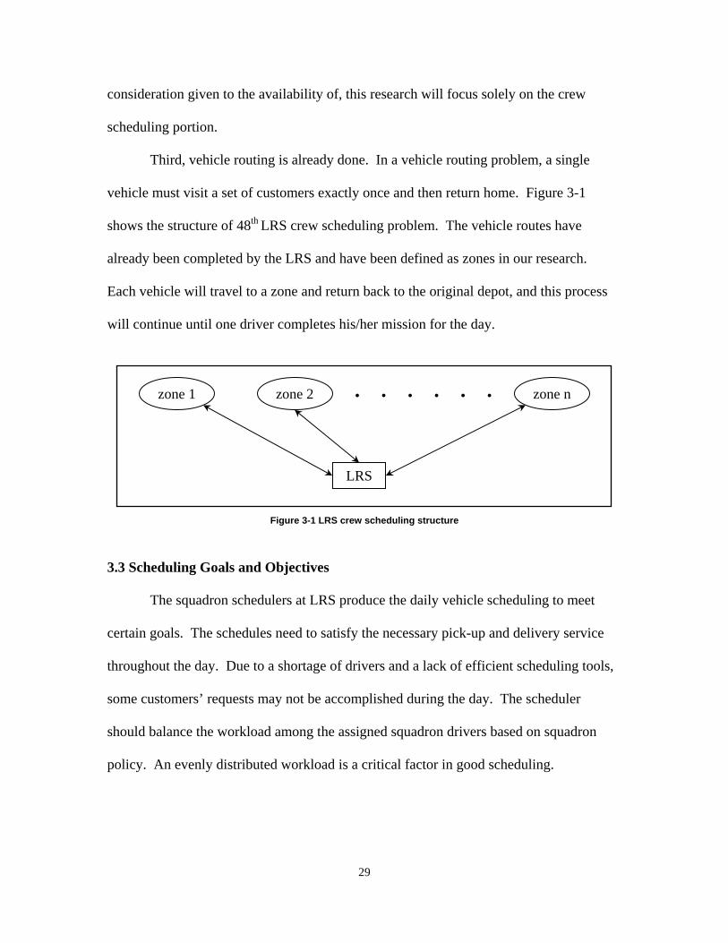
Third, vehicle routing is already done. In a vehicle routing problem, a single

vehicle must visit a set of customers exactly once and then return home. Figure 3-1

shows the structure of 48th LRS crew scheduling problem. The vehicle routes have

already been completed by the LRS and have been defined as zones in our research.

Each vehicle will travel to a zone and return back to the original depot, and this process

will continue until one driver completes his/her mission for the day.

Figure 3-1 LRS crew scheduling structure

3.3 Scheduling Goals and Objectives

The squadron schedulers at LRS produce the daily vehicle scheduling to meet

certain goals. The schedules need to satisfy the necessary pick-up and delivery service

throughout the day. Due to a shortage of drivers and a lack of efficient scheduling tools,

some customers’ requests may not be accomplished during the day. The scheduler

should balance the workload among the assigned squadron drivers based on squadron

policy. An evenly distributed workload is a critical factor in good scheduling.

LRS

zone 1 zone 2 zone n • • • • • •

30

The overall objective for the VOE scheduler is to establish a robust schedule that

will both satisfy customer service demands and distribute work loads in a balanced

manner. The objective of this thesis is to provide a scheduling tool that is flexible, quick,

easy to use, and conductive to an optimal daily schedule.

3.4 Scheduling Model and Problem Characteristics

In order to understand the scheduling model, one must begin with an overview of

the scheduling process. The scheduling process in DSS can be summarized by the

following 5 steps.

1. Receive the daily recurring jobs and intermittent recurring jobs

2. Prioritize the jobs / check the availability of drivers and their qualification

3. Set up parameters for preparatory processing

4. Generate eligible duties

5. Generate a schedule

To produce a robust schedule, the scheduling environment has to be understood in

terms of its dynamic changes, scheduling requirements and other scheduling related

constraints. The operation environment at the 48th LRS is a fluid and dynamic

environment characterized by daily changing requirements. Requirements and priority

changes to schedules occur frequently, and this initiates a modification of the schedules.

For example, a driver might become ill and if there is no suitable substitute for the driver,

the schedule change is inevitable and may not accomplish certain customers’ requests.

31

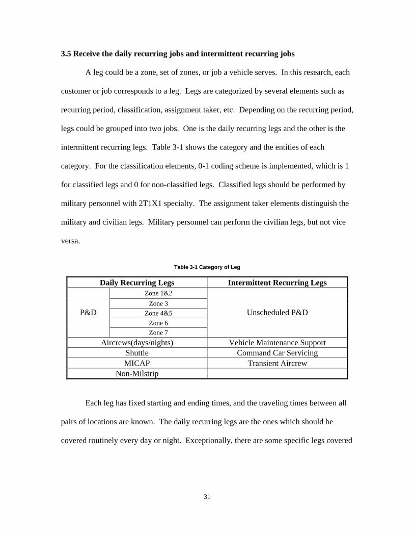
3.5 Receive the daily recurring jobs and intermittent recurring jobs

A leg could be a zone, set of zones, or job a vehicle serves. In this research, each

customer or job corresponds to a leg. Legs are categorized by several elements such as

recurring period, classification, assignment taker, etc. Depending on the recurring period,

legs could be grouped into two jobs. One is the daily recurring legs and the other is the

intermittent recurring legs. Table 3-1 shows the category and the entities of each

category. For the classification elements, 0-1 coding scheme is implemented, which is 1

for classified legs and 0 for non-classified legs. Classified legs should be performed by

military personnel with 2T1X1 specialty. The assignment taker elements distinguish the

military and civilian legs. Military personnel can perform the civilian legs, but not vice

versa.

Table 3-1 Category of Leg

Daily Recurring Legs Intermittent Recurring Legs Zone 1&2

Zone 3 Zone 4&5

Zone 6 P&D

Zone 7

Unscheduled P&D

Aircrews(days/nights) Vehicle Maintenance Support Shuttle Command Car Servicing MICAP Transient Aircrew

Non-Milstrip

Each leg has fixed starting and ending times, and the traveling times between all

pairs of locations are known. The daily recurring legs are the ones which should be

covered routinely every day or night. Exceptionally, there are some specific legs covered

32

only every Tuesday and Thursday only. However, the intermittent recurring legs are

unpredictable trips that may or may not result in changes in a predetermined schedule.

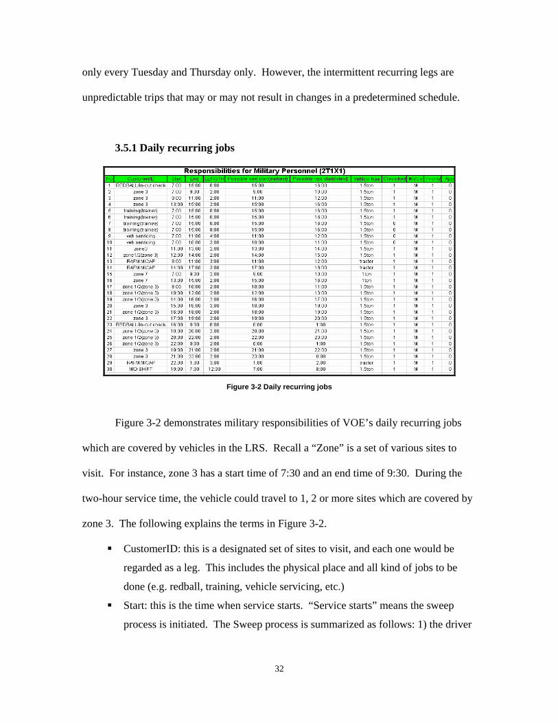
3.5.1 Daily recurring jobs

Figure 3-2 Daily recurring jobs

Figure 3-2 demonstrates military responsibilities of VOE’s daily recurring jobs

which are covered by vehicles in the LRS. Recall a “Zone” is a set of various sites to

visit. For instance, zone 3 has a start time of 7:30 and an end time of 9:30. During the

two-hour service time, the vehicle could travel to 1, 2 or more sites which are covered by

zone 3. The following explains the terms in Figure 3-2.

CustomerID: this is a designated set of sites to visit, and each one would be

regarded as a leg. This includes the physical place and all kind of jobs to be

done (e.g. redball, training, vehicle servicing, etc.)

Start: this is the time when service starts. “Service starts” means the sweep

process is initiated. The Sweep process is summarized as follows: 1) the driver

33

scans the property with the Supply Asset Tracking System (SATS) gun and

loads the property from the warehouse into the delivery vehicle. 2) the driver

travels to the delivery destination of property. 3) upon arrival at the destination,

the driver will find a “smart card” holder to sign for the property electronically

with SATS.

End: this is the time when service terminates and the driver is back at the depot.

Length: this is service duration.

Possible next start (earliest): this is the time considering the minimum rest time.

Possible next start (latest): this is the time considering the maximum rest time.

Vehicle type: in this thesis, we consider 5_types of vehicles (1ton, 1.5ton,

tractor, 19pax, 39pax), and there is no vehicle shortage for the duties.

Classified: classified requirement - 1, otherwise – 0

Mil/Civ: military or civilian driver requirement

Priority: prioritization of customers according to specific criteria (index from 1

to 3)

Appointment: this is job status designation as “Regular” or “Appointment”

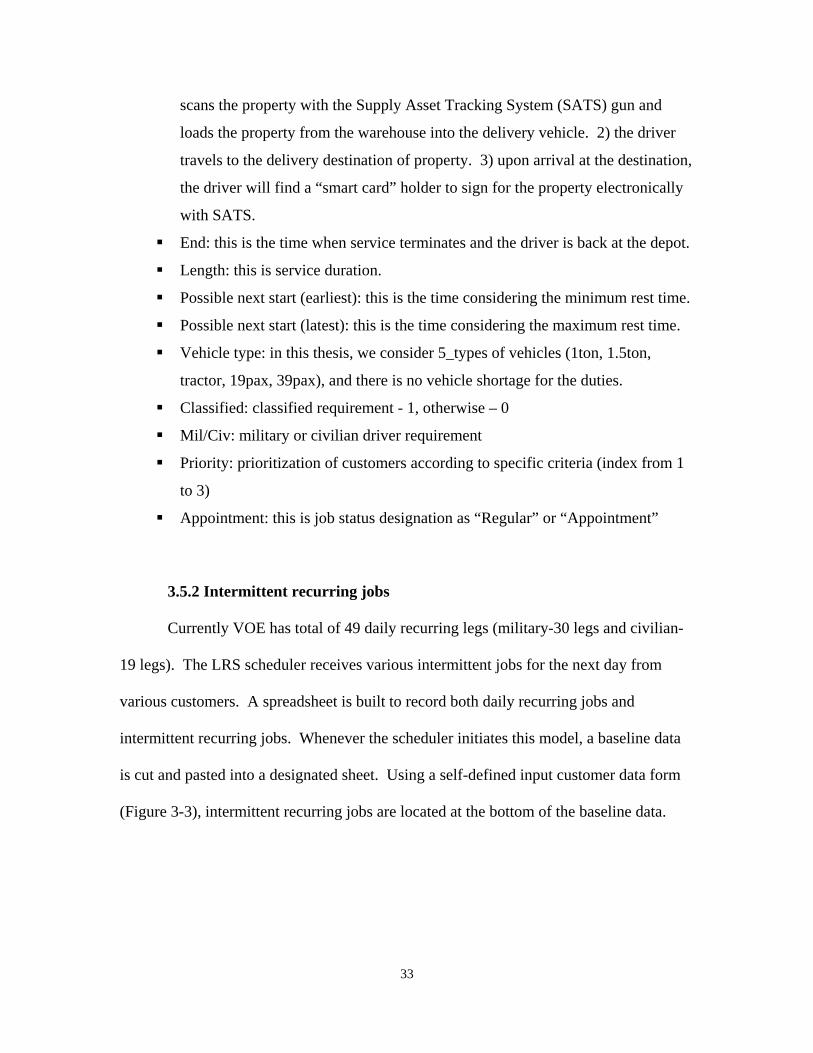
3.5.2 Intermittent recurring jobs

Currently VOE has total of 49 daily recurring legs (military-30 legs and civilian-

19 legs). The LRS scheduler receives various intermittent jobs for the next day from

various customers. A spreadsheet is built to record both daily recurring jobs and

intermittent recurring jobs. Whenever the scheduler initiates this model, a baseline data

is cut and pasted into a designated sheet. Using a self-defined input customer data form

(Figure 3-3), intermittent recurring jobs are located at the bottom of the baseline data.

34

Figure 3-3 Input Customer data (intermittent legs)

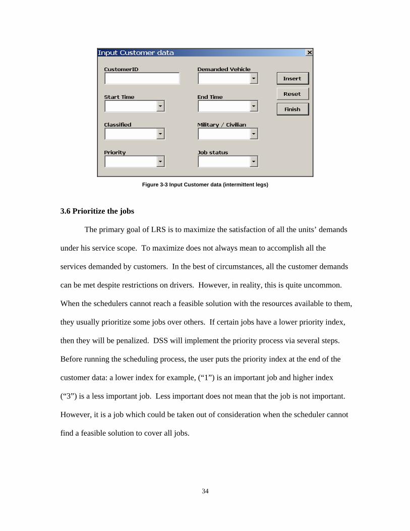
3.6 Prioritize the jobs

The primary goal of LRS is to maximize the satisfaction of all the units’ demands

under his service scope. To maximize does not always mean to accomplish all the

services demanded by customers. In the best of circumstances, all the customer demands

can be met despite restrictions on drivers. However, in reality, this is quite uncommon.

When the schedulers cannot reach a feasible solution with the resources available to them,

they usually prioritize some jobs over others. If certain jobs have a lower priority index,

then they will be penalized. DSS will implement the priority process via several steps.

Before running the scheduling process, the user puts the priority index at the end of the

customer data: a lower index for example, (“1”) is an important job and higher index

(“3”) is a less important job. Less important does not mean that the job is not important.

However, it is a job which could be taken out of consideration when the scheduler cannot

find a feasible solution to cover all jobs.

35

A Schedule result type has two options: 1) find the minimum number necessary

drivers, 2) find possible jobs with available drivers. The priority is associated with the

second option. Details will be covered at section 3.9.1 (Pricing Approach).

3.7 Check the availability of drivers and their qualification

The scheduler needs to keep track of available number of drivers and their

qualifications. Naturally, the status of a driver will have an impact on the next day’s

schedule. A driver might have a two-hour appointment with a doctor or might be on

leave. Those are predictable and the tracking is controllable things which must be

considered before processing the schedule. With this project, a limitation on personal

appointments during the shift time will be imposed. Each driver can have at most one

private appointment (e.g. dentist appointment or pick-up children, etc) under persuasive

document proof. DSS will process that appointment in the same fashion as regular legs.

3.8 Preparatory processing (parameter set-up)

Parameter setting is a prerequisite procedure for duty generation. It determines

which schedule strategy the scheduler will implement. Using the given parameters, DSS

will provide some insights about the schedule environment, such as lower bound of

necessary crew numbers or the best schedule scheme, etc.

36

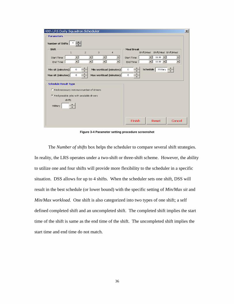
Figure 3-4 Parameter setting procedure screenshot

The Number of shifts box helps the scheduler to compare several shift strategies.

In reality, the LRS operates under a two-shift or three-shift scheme. However, the ability

to utilize one and four shifts will provide more flexibility to the scheduler in a specific

situation. DSS allows for up to 4 shifts. When the scheduler sets one shift, DSS will

result in the best schedule (or lower bound) with the specific setting of Min/Max sit and

Min/Max workload. One shift is also categorized into two types of one shift; a self

defined completed shift and an uncompleted shift. The completed shift implies the start

time of the shift is same as the end time of the shift. The uncompleted shift implies the

start time and end time do not match.

37

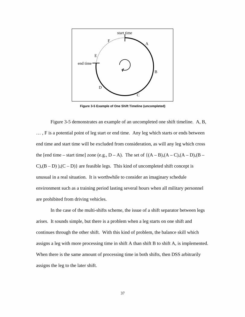
Figure 3-5 Example of One Shift Timeline (uncompleted)

Figure 3-5 demonstrates an example of an uncompleted one shift timeline. A, B,

… , F is a potential point of leg start or end time. Any leg which starts or ends between

end time and start time will be excluded from consideration, as will any leg which cross

the [end time – start time] zone (e.g., D – A). The set of {(A – B),(A – C),(A – D),(B –

C),(B – D) ),(C – D)} are feasible legs. This kind of uncompleted shift concept is

unusual in a real situation. It is worthwhile to consider an imaginary schedule

environment such as a training period lasting several hours when all military personnel

are prohibited from driving vehicles.

In the case of the multi-shifts scheme, the issue of a shift separator between legs

arises. It sounds simple, but there is a problem when a leg starts on one shift and

continues through the other shift. With this kind of problem, the balance skill which

assigns a leg with more processing time in shift A than shift B to shift A, is implemented.

When there is the same amount of processing time in both shifts, then DSS arbitrarily

assigns the leg to the later shift.

end time

A

B

C

D

start time

E

F

38

Min sit and Max sit – refer to the minimum and maximum connection time

between two consecutive legs in a duty. In reality, the LRS use 0 minutes for Min sit.

This implies that a driver could start another leg immediately after he or she finishes a

previous leg and returns to the depot. The Min sit and Max sit are not fixed variables.

The scheduler could change the values at the planning phase.

The definition of Min workload and Max workload for a day is intuitive. These

workloads exclude the meal break of 60 minutes (breakfast, lunch or dinner).

Throughout this research, the shift1 meal break (breakfast) time is between

5:00am and 7:00am, the shift2 meal break (lunch) time is between 11:30am and

13:30pm, and the shift3 meal break (dinner) time is between 17:30pm and 19:30pm.

When the scheduler makes a schedule with 4 shifts (6 hours each), the meal consideration

is ignored.

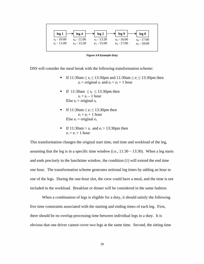
In Figure 3-6, a duty with a workload of 8 hours (480 minutes) is displayed. Each

si and ei is a start and end time of leg i. Intuitively, one may view this as a feasible duty,

but it is not. There is no time slot for a lunch break (assuming the consideration of lunch

meal break). The DSS meal break algorithm is based on several assumptions: 1) Max

workload for a day should not be more than 12 hours. 2) If a leg’s workload is greater

than 8 hours, the model does not apply meal considerations to the leg. For instance, a

“Training” leg is an 8-hour workload and the driver could finish a meal within the 8-hour

time slot. 3) Only a complete shift is considered. 4) Though a leg has a late breakfast

time and an early lunch time, the leg will have only a one-hour meal break when the

model considers both breakfast and lunch breaks.

39

Figure 3-6 Example Duty

DSS will consider the meal break with the following transformation scheme:

If 11:30am ≤ si ≤ 13:30pm and 11:30am ≤ ei ≤ 13:30pm then si = original si and ei = ei + 1 hour

If 11:30am ≤ si ≤ 13:30pm then si = si – 1 hour

Else si = original si

If 11:30am ≤ ei ≤ 13:30pm then ei = ei + 1 hour

Else ei = original ei

If 11:30am > si and ei > 13:30pm then ei = ei + 1 hour

This transformation changes the original start time, end time and workload of the leg,

assuming that the leg is in a specific time window (i.e., 11:30 – 13:30). When a leg starts

and ends precisely in the lunchtime window, the condition (1) will extend the end time

one hour. The transformation scheme generates notional leg times by adding an hour to

one of the legs. During the one-hour slot, the crew could have a meal, and the time is not

included in the workload. Breakfast or dinner will be considered in the same fashion.

When a combination of legs is eligible for a duty, it should satisfy the following

five time constraints associated with the starting and ending times of each leg. First,

there should be no overlap processing time between individual legs in a duty. It is

obvious that one driver cannot cover two legs at the same time. Second, the sitting time

leg 1

s1 - 10:00 e1 - 11:00

leg 4

s4 - 11:00 e4 - 13:30

leg 2

s2 - 13:30 e2 - 15:00

leg 9

s9 - 16:00 e9 - 17:00

leg 8

s8 - 17:00 e8 - 18:00

40

between legs should satisfy the Min sit and Max sit constraints. Third, the total workload

of a combination of legs should be within the range of Min workload and Max workload.

Fourth, the meal break between legs should be guaranteed. Finally, only legs in the same

shift may be combined into a specific duty.

3.9 Generate Eligible Duties

The tasks that are assigned to the same crew member define a crew duty.

Together the duties constitute a crew schedule. Duties consist of a number of legs (or

tasks) with a given maximum number of legs. In practice, this maximum is very often

equal to 2 or 3. In this research we put five legs as the maximum number of legs. In this

research, the terms of one-leg duty, two-leg duty, three-leg duty, four-leg duty, and five-

leg duty are defined as a crew duty consisting of n legs. The average leg length is

approximately 2 hours. Therefore to consider up to 5 legs (2 hours × 5 legs =10 hours) is

reasonable since an 8 hour shift is standard.

A duty is subject to 48th LRS Operation Instructions and LRS rules. The time

constraints associated with generating duties has already been mentioned in the previous

section (3.8 preparatory processing). Private duties such as a doctor’s appointment are

combined with regular duties. Classification constraints are comparatively

straightforward. Military personnel can handle both classified legs and non-classified

legs. However, civilian drivers like DoD and MoD employees, can be assigned to only

non-classified legs. DSS implements separate worksheets for daily and intermittent

recurring legs, and this approach leads to the separate consideration of military and

civilian jobs.

41

Generated duties are cornerstones for schedule generation. The next section will provide

a through discussion of the process of generating schedule.

3.10 Generating Schedule

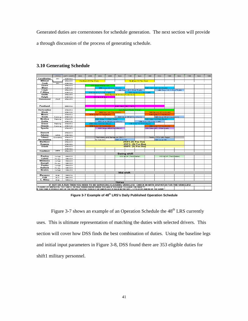
Figure 3-7 Example of 48th LRS’s Daily Published Operation Schedule

Figure 3-7 shows an example of an Operation Schedule the 48th LRS currently

uses. This is ultimate representation of matching the duties with selected drivers. This

section will cover how DSS finds the best combination of duties. Using the baseline legs

and initial input parameters in Figure 3-8, DSS found there are 353 eligible duties for

shift1 military personnel.

42

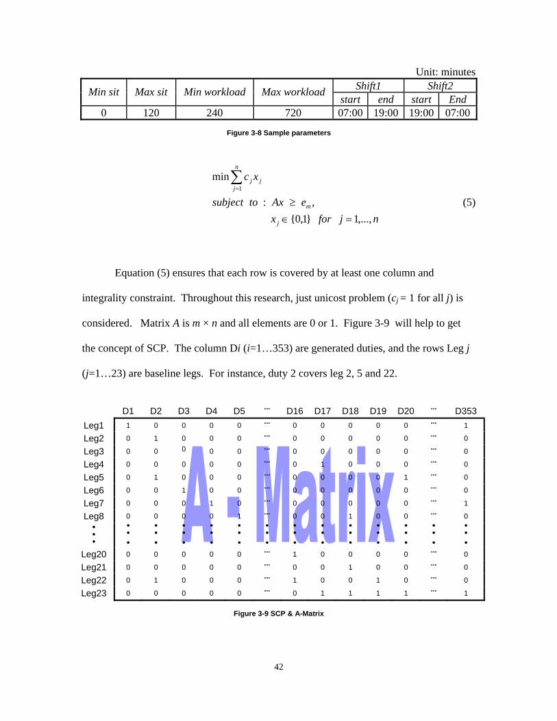
Unit: minutes Shift1 Shift2 Min sit Max sit Min workload Max workload

start end start End 0 120 240 720 07:00 19:00 19:00 07:00

Figure 3-8 Sample parameters

njforxeAxtosubject

xc

j

m

n

jjj

,...,1}1,0{,:

min1

=∈≥

∑=

(5)

Equation (5) ensures that each row is covered by at least one column and

integrality constraint. Throughout this research, just unicost problem (cj = 1 for all j) is

considered. Matrix A is m × n and all elements are 0 or 1. Figure 3-9 will help to get

the concept of SCP. The column Di (i=1…353) are generated duties, and the rows Leg j

(j=1…23) are baseline legs. For instance, duty 2 covers leg 2, 5 and 22.

D1 D2 D3 D4 D5 ··· D16 D17 D18 D19 D20 ··· D353

Leg1 1 0 0 0 0 ··· 0 0 0 0 0 ··· 1

Leg2 0 1 0 0 0 ··· 0 0 0 0 0 ··· 0

Leg3 0 0 0 0 0 ··· 0 0 0 0 0 ··· 0

Leg4 0 0 0 0 0 ··· 0 1 0 0 0 ··· 0

Leg5 0 1 0 0 0 ··· 0 0 0 0 1 ··· 0

Leg6 0 0 1 0 0 ··· 0 0 0 0 0 ··· 0

Leg7 0 0 0 1 0 ··· 0 0 0 0 0 ··· 1

Leg8 0 0 0 0 1 ··· 0 0 1 0 0 ··· 0 • • •

• • •

• • •

• • •

• • •

• • •

• • •

• • •

• • •

• • •

• • •

• • •

• • •

• • •

Leg20 0 0 0 0 0 ··· 1 0 0 0 0 ··· 0

Leg21 0 0 0 0 0 ··· 0 0 1 0 0 ··· 0

Leg22 0 1 0 0 0 ··· 1 0 0 1 0 ··· 0

Leg23 0 0 0 0 0 ··· 0 1 1 1 1 ··· 1

Figure 3-9 SCP & A-Matrix

43

There are many algorithms and pertinent literatures for solving SCP as the reader

can see in the chapter 2. DSS uses the Premium Excel Solver (PES) and SA to get a

feasible schedule. Unfortunately, the PES could only handle 200 columns at a time.

When the total number of generated duties is less than or equal to 200, no problems arise.

However, if it is not the case, then DSS needs tool for solving that kind of problem. For

instance, if the DSS results in 353 duties, then the PES will solve the problem with 200

columns and find solution. The solution might be better when considering the extra 153

duties instead of the duties already evaluated in PES.

3.10.1 Pricing Approach

It is assumed that the reader is already familiar with the Excel Solver and

Sensitivity Report in Solver. Sensitivity Report shows the original and final values of the

objective function and the decision variables, as well as the status of each constraint at

the optimal solution.

Pricing approach uses the Microsoft Office’s student version of Premium Excel

Solver (PES) and that has three different built-in engines to solve the problem. Those

three engines are Standard GRG Nonlinear, Standard Simplex LP, and Standard

Evolutionary. To use the concept of reduced cost and shadow price, “Standard Simplex

LP” engine is implemented. Unfortunately, the PES could only handle 200 variables at a

time. When the total number of generated duties is less than or equal to 200, no problems

arise. However, if it is not the case, then DSS needs a tool for solving that kind of

problem. Advanced solver version (e.g. Premium Solver Platform) could handle up to

2000 linear variables and 8000 constraints. However, the software package is not free.

44

This kind of financial issue also leads the military users to utilize the built-in engines.

The DSS model uses the built–in standard solver engine and modifies to get a solution.

For instance, if the DSS results in 353 duties, then the PES will solve the problem with

200 columns and find a solution. The solution might be better when considering the extra

153 duties instead of the duties already evaluated in PES. It sounds like sensitivity

analysis. Suppose that the simplex method produced an optimal basis B with current 200

duties. The point is how to make use of the optimality conditions (primal-dual

relationships) in order to find the new optimal solution, if some of the problem data

change, without resolving the problem from scratch. In particular, the following

variations in the problem could be considered.

Change in the cost vector c.

Change in the right-hand-side vector b.

Change in the constraint matrix A.

Addition of a new duty.

Addition of a new leg.

Among those variations, pricing algorithm is associated with “Addition of a new duty”.

Suppose that a new duty Dn+1 with unit cost cn+1 and consumption column an+1 is

considered for possible production. Without resolving the problem, it could be easily

determined whether producing Dn+1 is worthwhile. First calculate zn+1 – cn+1. If zn+1 –

cn+1 ≤ 0, then D*n+1 = 0 and the current solution is optimal. On the other hand, if zn+1 –

cn+1 > 0, then Dn+1 is introduced into the basis and the simplex method continues to find

the new optimal solution. The pricing algorithm which is built in DSS will be explained

in detail below.

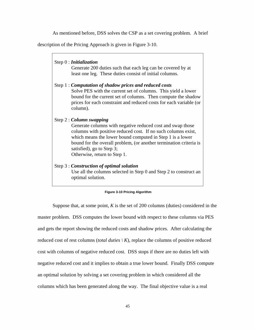
45

As mentioned before, DSS solves the CSP as a set covering problem. A brief

description of the Pricing Approach is given in Figure 3-10.

Step 0 : Initialization

Generate 200 duties such that each leg can be covered by at least one leg. These duties consist of initial columns.

Step 1 : Computation of shadow prices and reduced costs

Solve PES with the current set of columns. This yield a lower bound for the current set of columns. Then compute the shadow prices for each constraint and reduced costs for each variable (or column).

Step 2 : Column swapping

Generate columns with negative reduced cost and swap those columns with positive reduced cost. If no such columns exist, which means the lower bound computed in Step 1 is a lower bound for the overall problem, (or another termination criteria is satisfied), go to Step 3; Otherwise, return to Step 1.

Step 3 : Construction of optimal solution

Use all the columns selected in Step 0 and Step 2 to construct an optimal solution.

Figure 3-10 Pricing Algorithm

Suppose that, at some point, K is the set of 200 columns (duties) considered in the

master problem. DSS computes the lower bound with respect to these columns via PES

and gets the report showing the reduced costs and shadow prices. After calculating the

reduced cost of rest columns (total duties \ K), replace the columns of positive reduced

cost with columns of negative reduced cost. DSS stops if there are no duties left with

negative reduced cost and it implies to obtain a true lower bound. Finally DSS compute

an optimal solution by solving a set covering problem in which considered all the

columns which has been generated along the way. The final objective value is a real

46

number, and DSS get the integer objective value via adding integrality and lower bound

value into the constraints. To avoid overlapping legs at most, DSS uses different solver

setting and resolve the problem. This procedure results in maintaining the same amount

of drivers (first objective value) and simultaneously minimizing the number of

overlapping legs (second objective value). Figure 3-11 and Figure 3-12 illustrate the

solver parameters setting for generating an optimal solution and avoiding overlapped

legs, respectively. Avoiding overlapping is a way to transform the set covering problem

(SCP) to set partitioning problem (SPP). However, this method does not always

guarantee the non-overlapping. Because the optimal solution is generated from SCP not

SPP.

By now, pricing algorithm to find optimal solution was detailed. The advantage

of DSS model is to use this model as analysis tool. The scheduler may wonder “How

many legs could we handle with current status of drivers?” The B-Matrix and priority of

each leg do a significant job with this sort of situation. The A-Matrix does not consider

the priority of each leg or just assumes they are all “1”, which means should be done for

next day. The A-Matrix and B-Matrix are self-defined terms for sub procedure of DSS

model. The scheduler could get the optimal drivers amount with the processing of A-

Matrix. If the optimal number is less than the current available driver number, then it

will be fine. If not, the scheduler would try to minimize the penalty of not satisfying all

the requested jobs. Legs with high priority have 105 penalty, 103 for medium priority

legs, and 10 for the low priority legs. The processing of B-Matrix results in how many

legs with each priority could not be satisfied and what the legs are. Simultaneously, the

result schedule has the evenly distributed work load among drivers.

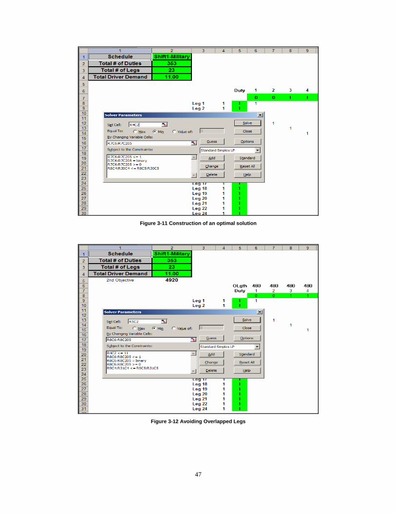
47

Figure 3-11 Construction of an optimal solution

Figure 3-12 Avoiding Overlapped Legs

48

3.10.2 Heuristic (Simulated Annealing)

The meta heuristic Simulated Annealing combined with Set Covering Problem

(SCP) is also implemented here to find the minimum duty number to cover all legs. As

mentioned in chapter 2, SA has four elements to consider. They are representations of

possible solutions, generator of random changes in solutions, means of evaluating the

problem functions, and annealing schedule.

3.10.2.1 Representations of possible solutions

‘Possible solutions’ is not an ultimate solution but a solution for PES. With this

solution the Excel runs the premium solver and produces an ultimate solution for DSS.

The SA starts its process with random initial solution. The better the initial solution is,

the less processing time takes. Two points are intuitive at selecting initial solution: 1) all

only-one-leg duties should be included in the 200 duties for PES. An only-one-leg duty

is a duty which has no room for other legs. Therefore, there is no two-leg duty

combining the only-one-leg duty with other leg. 2) Five-leg duties are more efficient

than one or two-leg duties. There might be an arguing point here, however in general it

does make sense when considering initial solution.

‘On duty array’ (Figure 3-13) is a set of 200 duties which is chosen for the PES.

Considering the two points mentioned above, DSS generates an initial solution, and

checks whether the chosen duties cover all legs. If the ‘on duty array’ does not satisfy

feasibility conditions, then random duties are chosen from the ‘off duty array’ switched

with duties from the ‘on duty array’ and then checked for feasibility. This process

continues until a feasible solution for PES is found.

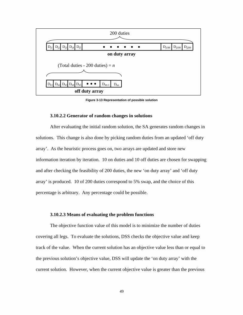
49

Figure 3-13 Representation of possible solution

3.10.2.2 Generator of random changes in solutions

After evaluating the initial random solution, the SA generates random changes in

solutions. This change is also done by picking random duties from an updated ‘off duty

array’. As the heuristic process goes on, two arrays are updated and store new

information iteration by iteration. 10 on duties and 10 off duties are chosen for swapping

and after checking the feasibility of 200 duties, the new ‘on duty array’ and ‘off duty

array’ is produced. 10 of 200 duties correspond to 5% swap, and the choice of this

percentage is arbitrary. Any percentage could be possible.

3.10.2.3 Means of evaluating the problem functions

The objective function value of this model is to minimize the number of duties

covering all legs. To evaluate the solutions, DSS checks the objective value and keep

track of the value. When the current solution has an objective value less than or equal to

the previous solution’s objective value, DSS will update the ‘on duty array’ with the

current solution. However, when the current objective value is greater than the previous

• • • • • •on duty array

off duty array

Dj1 Dj2 Dj3 Dj4 Dj5 Dj198 Dj199 Dj200

200 duties

• • • Dk1 Dk2 Dk3 Dk4 Dk5 Dkn Dkn-1

(Total duties - 200 duties) = n

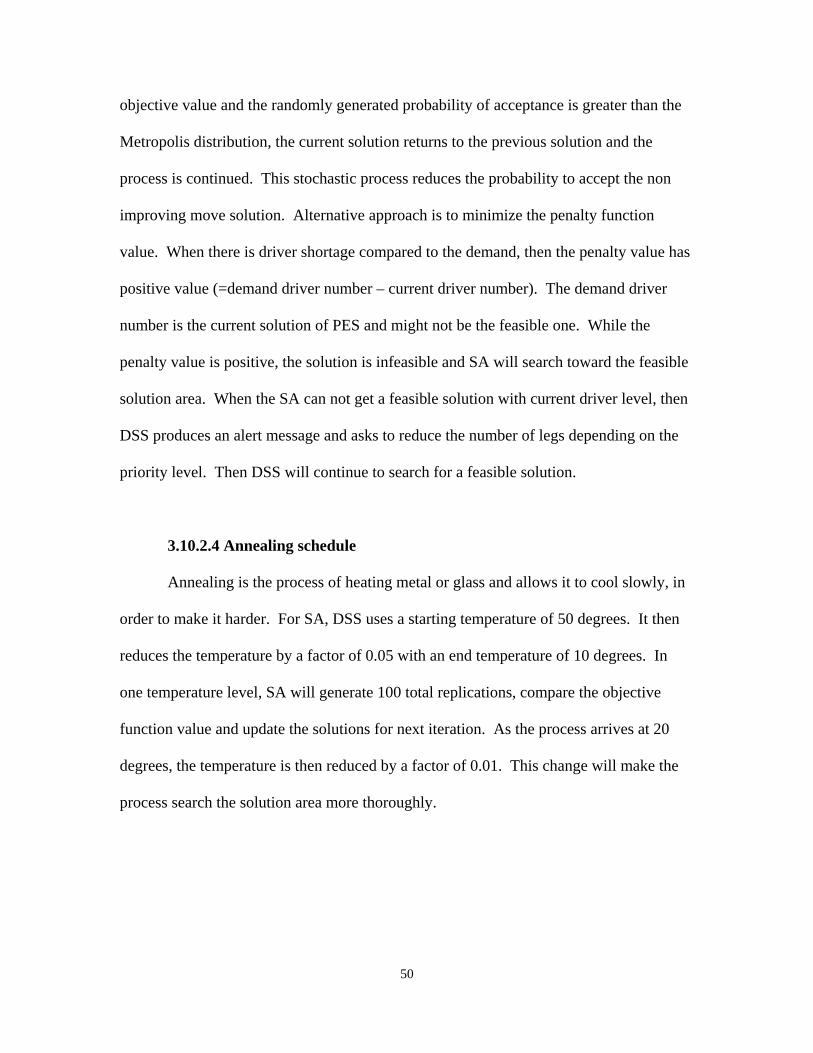
50

objective value and the randomly generated probability of acceptance is greater than the

Metropolis distribution, the current solution returns to the previous solution and the

process is continued. This stochastic process reduces the probability to accept the non

improving move solution. Alternative approach is to minimize the penalty function

value. When there is driver shortage compared to the demand, then the penalty value has

positive value (=demand driver number – current driver number). The demand driver

number is the current solution of PES and might not be the feasible one. While the

penalty value is positive, the solution is infeasible and SA will search toward the feasible

solution area. When the SA can not get a feasible solution with current driver level, then

DSS produces an alert message and asks to reduce the number of legs depending on the

priority level. Then DSS will continue to search for a feasible solution.

3.10.2.4 Annealing schedule

Annealing is the process of heating metal or glass and allows it to cool slowly, in

order to make it harder. For SA, DSS uses a starting temperature of 50 degrees. It then

reduces the temperature by a factor of 0.05 with an end temperature of 10 degrees. In

one temperature level, SA will generate 100 total replications, compare the objective

function value and update the solutions for next iteration. As the process arrives at 20

degrees, the temperature is then reduced by a factor of 0.01. This change will make the

process search the solution area more thoroughly.

51

3.11 Summary

This chapter presented the methodology for solving the squadron-scheduling

problem. The pricing algorithm provides lower bound for the required number of drivers

(first objective value) and also builds least overlapped scheduling plan (second objective

value). The scheduling process in DSS can be summarized by the 5 steps. 1) The

scheduler starts the DSS by building appropriate parameter. In reality, the scheduling

parameter is fixed during some specific time period. The scheduler could use this model

as an analysis tool for future working environment. 2) Receive the daily recurring jobs

and intermittent recurring jobs. This step could be done simultaneously with step 3)

Prioritize the jobs / check the availability of drivers and their qualification. Daily

recurring jobs have priority 1, which means those jobs should be done. However, the

intermittent jobs’ priority is dependent on the scheduler. This model provides the tool for

checking the feasibility whether the VOE could handle the whole requirements from

every customer under current drivers status. 4) Generate eligible duties. Eligible duties

are those which satisfy the parameter set-up conditions (e.g., shift time, meal

consideration, sit time, work load, etc). 5) Generate a schedule. This is the final step for

DSS. Next chapter details how the methodology was tested and the results of this testing.

52

Chapter 4. Analysis and Results 4.1 Chapter Overview

This chapter describes the analysis of the schedules generated to meet the current

scheduling environment. The development of the Daily Squadron Scheduler required

testing to ensure that the model performed quickly and could solve the appropriate

problems. This chapter is broken up into two sections. The first section analyzes various

scheduling scheme and their results with current daily recurring jobs. The second section

sets up many notional delivery scheduling composed with daily recurring jobs plus

various intermittent jobs, and analyze the results.

4.2 Physical Structures and the Performance of the Software

The software design can be measured by looking at the interface environment and

the flexibility of the software in the scheduling generation process. The software

interface environment is straightforward and user friendly. DSS is composed of eight

worksheets. “Explanation” is the main menu provides a list of choices for the user to

enter parameter setup, copy the daily recurring jobs, input legs data into formatted

spreadsheet, execute the model or exit the program completely. Figure 4-1 shows the

start up menu. “LRS DATA” is baseline spreadsheet containing daily recurring jobs both

military and civilian. Whenever there is a change with daily recurring jobs, the scheduler

could update manually the data in the spreadsheet. This information will be

53

Figure 4-1 Start Up Menu

automatically copied at “Customer for Military Personnel” or “Customer for Civilian

Drivers” when create new customers button in the User Option form is executed.

“Customer for Military Personnel” and “Customer for Civilian Drivers” are spreadsheet

for containing the leg data for military and civilian respectively. The Excel spreadsheet

allows manual overrides of most functions to provide the squadron scheduler with

maximum flexibility. The scheduler input intermittent recurring jobs into the spreadsheet

either using main menu or writing directly on the spreadsheet. “A-Matrix” is used for

calculating the optimal number of required drivers and “B-Matrix” is used for figuring

out the possible legs with current driver number. Throughout the processing, the

scheduler could trace the results of objective function value as Solver updates the value at

the specific cell in “A-Matrix” or “B-Matrix”. “Total Schedule” and “Answer Report”

are the results of schedule and its statistics for the schedule, respectively.

54

4.3 Parameters Analysis

Note that both meta heuristic SA algorithm and pricing algorithm are introduced

in chapter 3. As some sample problems are implemented under the SA algorithm, several

significant facts were found. First, the heuristic generates the solution based on

randomization. At one temperature, the algorithm explores the solution space, picks a

specific solution randomly and selects the solution according to the improvement

condition or probability. After a fixed number of iterations, it will be cooled and the

process will be continued until the temperature reaches the preset degree. This kind of

approach is seriously time-consuming as the problem size increases dramatically. Second,

it can be shown that, for any given finite problem, the probability that the simulated

annealing algorithm terminates with the global optimal solution approaches 1 as the

annealing schedule is extended. This theoretical result is, however, not particularly

helpful, since the annealing time required to ensure a significant probability of success

will usually exceed the time required for a complete search of the solution space. Third,

theoretically, the SA will converge to the optimal solution given an appropriate cooling

schedule. Without the appropriate cooling schedule, the optimality could not be

guaranteed. Thus, the solution of SA is not good as the one which is resulted from

pricing algorithm. Therefore, only pricing algorithm results will be analyzed throughout

this chapter.

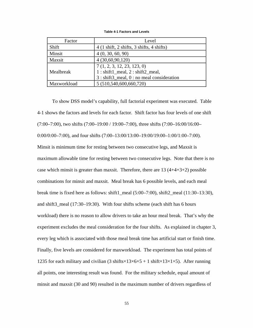
55

Table 4-1 Factors and Levels

Factor Level Shift 4 (1 shift, 2 shifts, 3 shifts, 4 shifts) Minsit 4 (0, 30, 60, 90) Maxsit 4 (30,60,90,120)

Mealbreak 7 (1, 2, 3, 12, 23, 123, 0) 1 : shift1_meal, 2 : shift2_meal, 3 : shift3_meal, 0 : no meal consideration

Maxworkload 5 (510,540,600,660,720)

To show DSS model’s capability, full factorial experiment was executed. Table

4-1 shows the factors and levels for each factor. Shift factor has four levels of one shift

(7:00–7:00), two shifts (7:00–19:00 / 19:00–7:00), three shifts (7:00–16:00/16:00–

0:00/0:00–7:00), and four shifts (7:00–13:00/13:00–19:00/19:00–1:00/1:00–7:00).

Minsit is minimum time for resting between two consecutive legs, and Maxsit is

maximum allowable time for resting between two consecutive legs. Note that there is no

case which minsit is greater than maxsit. Therefore, there are 13 (4+4+3+2) possible

combinations for minsit and maxsit. Meal break has 6 possible levels, and each meal

break time is fixed here as follows: shift1_meal (5:00–7:00), shift2_meal (11:30–13:30),

and shift3_meal (17:30–19:30). With four shifts scheme (each shift has 6 hours

workload) there is no reason to allow drivers to take an hour meal break. That’s why the

experiment excludes the meal consideration for the four shifts. As explained in chapter 3,

every leg which is associated with those meal break time has artificial start or finish time.

Finally, five levels are considered for maxworkload. The experiment has total points of

1235 for each military and civilian (3 shifts×13×6×5 + 1 shift×13×1×5). After running

all points, one interesting result was found. For the military schedule, equal amount of

minsit and maxsit (30 and 90) resulted in the maximum number of drivers regardless of

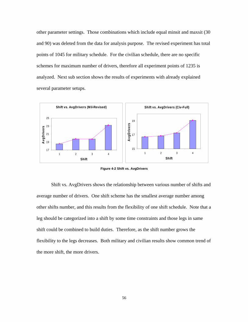
56

other parameter settings. Those combinations which include equal minsit and maxsit (30

and 90) was deleted from the data for analysis purpose. The revised experiment has total

points of 1045 for military schedule. For the civilian schedule, there are no specific

schemes for maximum number of drivers, therefore all experiment points of 1235 is

analyzed. Next sub section shows the results of experiments with already explained

several parameter setups.

Shift vs. AvgDrivers (Mil-Revised)

17

19

21

23

25

1 2 3 4

Shift

Avg

Driv

ers

Shift vs. AvgDrivers (Civ-Full)

15

17

19

1 2 3 4

Shift

Avg

Driv

ers

Figure 4-2 Shift vs. AvgDrivers

Shift vs. AvgDrivers shows the relationship between various number of shifts and

average number of drivers. One shift scheme has the smallest average number among

other shifts number, and this results from the flexibility of one shift schedule. Note that a

leg should be categorized into a shift by some time constraints and those legs in same

shift could be combined to build duties. Therefore, as the shift number grows the

flexibility to the legs decreases. Both military and civilian results show common trend of

the more shift, the more drivers.

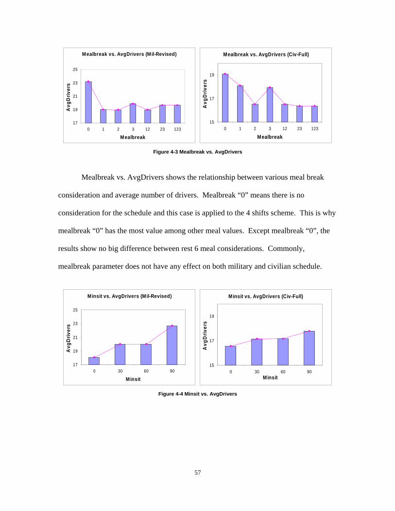
57

Mealbreak vs. AvgDrivers (Mil-Revised)

17

19

21

23

25

0 1 2 3 12 23 123

Mealbreak

Avg

Driv

ers

Mealbreak vs. AvgDrivers (Civ-Full)

15

17

19

0 1 2 3 12 23 123

Mealbreak

Avg

Driv

ers

Figure 4-3 Mealbreak vs. AvgDrivers

Mealbreak vs. AvgDrivers shows the relationship between various meal break

consideration and average number of drivers. Mealbreak “0” means there is no

consideration for the schedule and this case is applied to the 4 shifts scheme. This is why

mealbreak “0” has the most value among other meal values. Except mealbreak “0”, the

results show no big difference between rest 6 meal considerations. Commonly,

mealbreak parameter does not have any effect on both military and civilian schedule.

Minsit vs. AvgDrivers (Mil-Revised)

17

19

21

23

25

0 30 60 90

Minsit

Avg

Driv

ers

Minsit vs. AvgDrivers (Civ-Full)

15

17

19

0 30 60 90Minsit

Avg

Driv

ers

Figure 4-4 Minsit vs. AvgDrivers

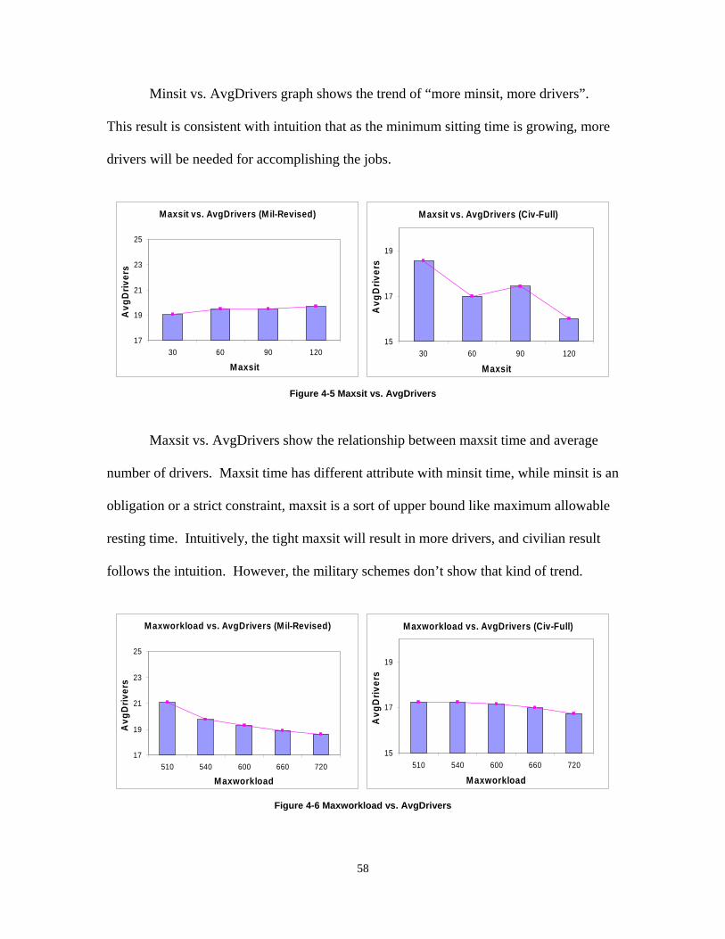
58

Minsit vs. AvgDrivers graph shows the trend of “more minsit, more drivers”.

This result is consistent with intuition that as the minimum sitting time is growing, more

drivers will be needed for accomplishing the jobs.

Maxsit vs. AvgDrivers (Mil-Revised)

17

19

21

23

25

30 60 90 120

Maxsit

Avg

Driv

ers

Maxsit vs. AvgDrivers (Civ-Full)

15

17

19

30 60 90 120

MaxsitA

vgD

river

s

Figure 4-5 Maxsit vs. AvgDrivers

Maxsit vs. AvgDrivers show the relationship between maxsit time and average

number of drivers. Maxsit time has different attribute with minsit time, while minsit is an

obligation or a strict constraint, maxsit is a sort of upper bound like maximum allowable

resting time. Intuitively, the tight maxsit will result in more drivers, and civilian result

follows the intuition. However, the military schemes don’t show that kind of trend.

Maxworkload vs. AvgDrivers (Mil-Revised)

17

19

21

23

25

510 540 600 660 720

Maxworkload

Avg

Driv

ers

Maxworkload vs. AvgDrivers (Civ-Full)

15

17

19

510 540 600 660 720

Maxworkload

Avg

Driv

ers

Figure 4-6 Maxworkload vs. AvgDrivers

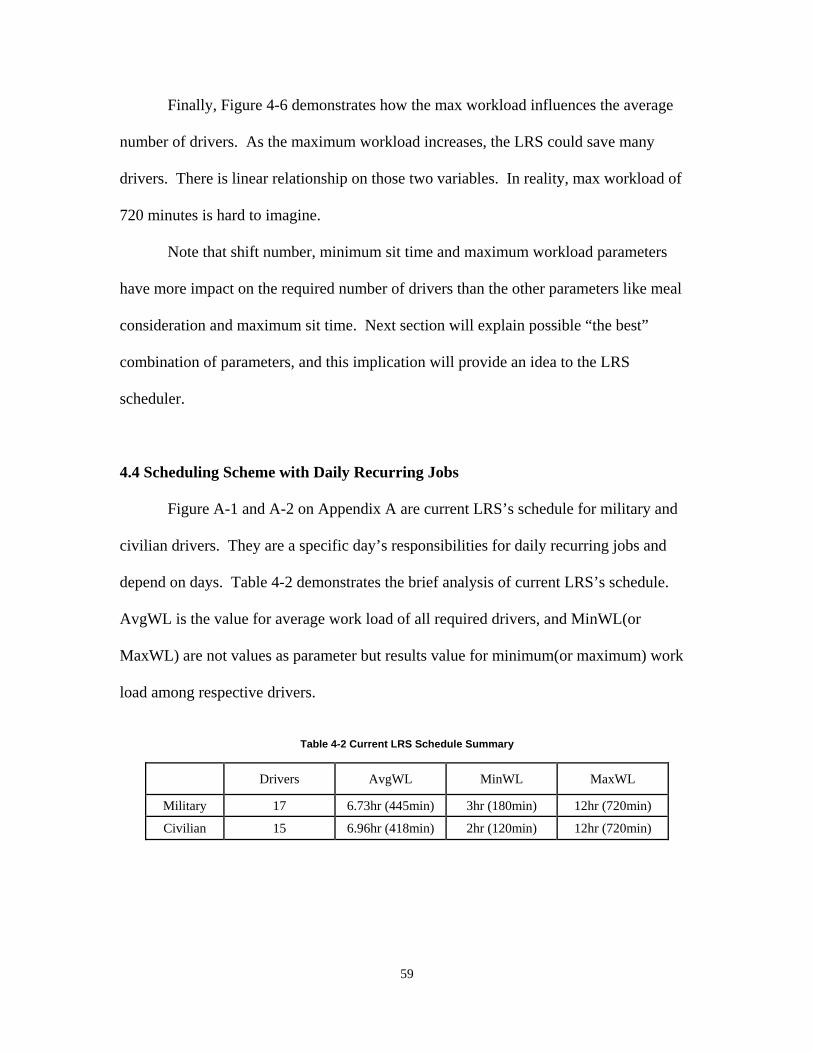
59

Finally, Figure 4-6 demonstrates how the max workload influences the average

number of drivers. As the maximum workload increases, the LRS could save many

drivers. There is linear relationship on those two variables. In reality, max workload of

720 minutes is hard to imagine.

Note that shift number, minimum sit time and maximum workload parameters

have more impact on the required number of drivers than the other parameters like meal

consideration and maximum sit time. Next section will explain possible “the best”

combination of parameters, and this implication will provide an idea to the LRS

scheduler.

4.4 Scheduling Scheme with Daily Recurring Jobs

Figure A-1 and A-2 on Appendix A are current LRS’s schedule for military and

civilian drivers. They are a specific day’s responsibilities for daily recurring jobs and

depend on days. Table 4-2 demonstrates the brief analysis of current LRS’s schedule.

AvgWL is the value for average work load of all required drivers, and MinWL(or

MaxWL) are not values as parameter but results value for minimum(or maximum) work

load among respective drivers.

Table 4-2 Current LRS Schedule Summary

Drivers AvgWL MinWL MaxWL

Military 17 6.73hr (445min) 3hr (180min) 12hr (720min)

Civilian 15 6.96hr (418min) 2hr (120min) 12hr (720min)

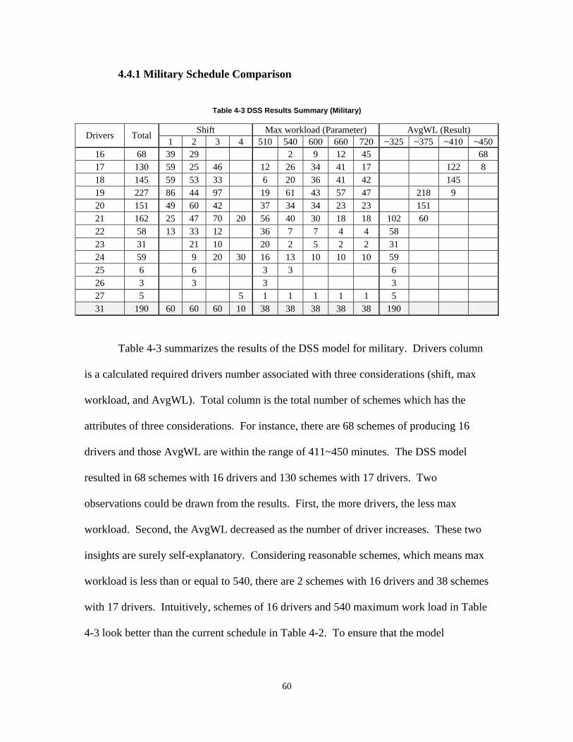
60

4.4.1 Military Schedule Comparison

Table 4-3 DSS Results Summary (Military)

Shift Max workload (Parameter) AvgWL (Result) Drivers Total 1 2 3 4 510 540 600 660 720 ~325 ~375 ~410 ~450

16 68 39 29 2 9 12 45 68 17 130 59 25 46 12 26 34 41 17 122 8 18 145 59 53 33 6 20 36 41 42 145 19 227 86 44 97 19 61 43 57 47 218 9 20 151 49 60 42 37 34 34 23 23 151 21 162 25 47 70 20 56 40 30 18 18 102 60 22 58 13 33 12 36 7 7 4 4 58 23 31 21 10 20 2 5 2 2 31 24 59 9 20 30 16 13 10 10 10 59 25 6 6 3 3 6 26 3 3 3 3 27 5 5 1 1 1 1 1 5 31 190 60 60 60 10 38 38 38 38 38 190

Table 4-3 summarizes the results of the DSS model for military. Drivers column

is a calculated required drivers number associated with three considerations (shift, max

workload, and AvgWL). Total column is the total number of schemes which has the

attributes of three considerations. For instance, there are 68 schemes of producing 16

drivers and those AvgWL are within the range of 411~450 minutes. The DSS model

resulted in 68 schemes with 16 drivers and 130 schemes with 17 drivers. Two

observations could be drawn from the results. First, the more drivers, the less max

workload. Second, the AvgWL decreased as the number of driver increases. These two

insights are surely self-explanatory. Considering reasonable schemes, which means max

workload is less than or equal to 540, there are 2 schemes with 16 drivers and 38 schemes

with 17 drivers. Intuitively, schemes of 16 drivers and 540 maximum work load in Table

4-3 look better than the current schedule in Table 4-2. To ensure that the model

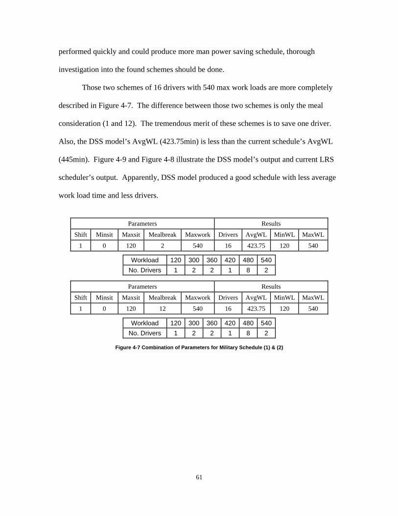
61

performed quickly and could produce more man power saving schedule, thorough

investigation into the found schemes should be done.

Those two schemes of 16 drivers with 540 max work loads are more completely

described in Figure 4-7. The difference between those two schemes is only the meal

consideration (1 and 12). The tremendous merit of these schemes is to save one driver.

Also, the DSS model’s AvgWL (423.75min) is less than the current schedule’s AvgWL

(445min). Figure 4-9 and Figure 4-8 illustrate the DSS model’s output and current LRS

scheduler’s output. Apparently, DSS model produced a good schedule with less average

work load time and less drivers.

Parameters Results

Shift Minsit Maxsit Mealbreak Maxwork Drivers AvgWL MinWL MaxWL

1 0 120 2 540 16 423.75 120 540

Workload 120 300 360 420 480 540No. Drivers 1 2 2 1 8 2

Parameters Results

Shift Minsit Maxsit Mealbreak Maxwork Drivers AvgWL MinWL MaxWL

1 0 120 12 540 16 423.75 120 540

Workload 120 300 360 420 480 540No. Drivers 1 2 2 1 8 2

Figure 4-7 Combination of Parameters for Military Schedule (1) & (2)

62

Figure 4-8 LRS Current Military Schedule

Figure 4-9 DSS Military Schedule (1)

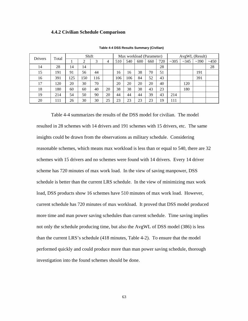
63

4.4.2 Civilian Schedule Comparison

Table 4-4 DSS Results Summary (Civilian)

Shift Max workload (Parameter) AvgWL (Result) Drivers Total 1 2 3 4 510 540 600 660 720 ~305 ~345 ~390 ~450

14 28 14 14 28 28 15 191 91 56 44 16 16 38 70 51 191 16 391 125 150 116 106 106 84 52 43 391 17 120 20 30 70 20 20 20 20 40 120 18 180 60 60 40 20 38 38 38 43 23 180 19 214 54 50 90 20 44 44 44 39 43 214 20 111 26 30 30 25 23 23 23 23 19 111

Table 4-4 summarizes the results of the DSS model for civilian. The model

resulted in 28 schemes with 14 drivers and 191 schemes with 15 drivers, etc. The same

insights could be drawn from the observations as military schedule. Considering

reasonable schemes, which means max workload is less than or equal to 540, there are 32

schemes with 15 drivers and no schemes were found with 14 drivers. Every 14 driver

scheme has 720 minutes of max work load. In the view of saving manpower, DSS

schedule is better than the current LRS schedule. In the view of minimizing max work

load, DSS products show 16 schemes have 510 minutes of max work load. However,

current schedule has 720 minutes of max workload. It proved that DSS model produced

more time and man power saving schedules than current schedule. Time saving implies

not only the schedule producing time, but also the AvgWL of DSS model (386) is less

than the current LRS’s schedule (418 minutes, Table 4-2). To ensure that the model

performed quickly and could produce more than man power saving schedule, thorough

investigation into the found schemes should be done.

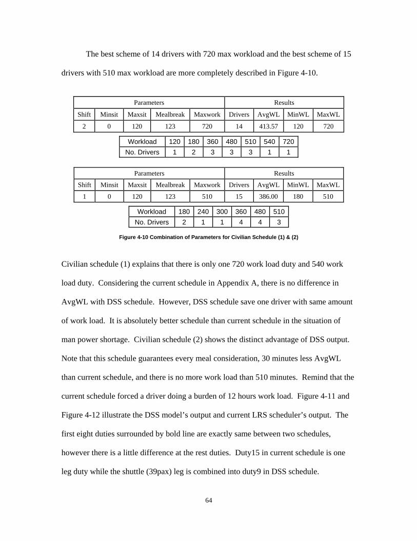
64

The best scheme of 14 drivers with 720 max workload and the best scheme of 15

drivers with 510 max workload are more completely described in Figure 4-10.

Parameters Results

Shift Minsit Maxsit Mealbreak Maxwork Drivers AvgWL MinWL MaxWL

2 0 120 123 720 14 413.57 120 720

Workload 120 180 360 480 510 540 720 No. Drivers 1 2 3 3 3 1 1

Parameters Results

Shift Minsit Maxsit Mealbreak Maxwork Drivers AvgWL MinWL MaxWL

1 0 120 123 510 15 386.00 180 510

Workload 180 240 300 360 480 510No. Drivers 2 1 1 4 4 3

Figure 4-10 Combination of Parameters for Civilian Schedule (1) & (2)

Civilian schedule (1) explains that there is only one 720 work load duty and 540 work

load duty. Considering the current schedule in Appendix A, there is no difference in

AvgWL with DSS schedule. However, DSS schedule save one driver with same amount

of work load. It is absolutely better schedule than current schedule in the situation of

man power shortage. Civilian schedule (2) shows the distinct advantage of DSS output.

Note that this schedule guarantees every meal consideration, 30 minutes less AvgWL

than current schedule, and there is no more work load than 510 minutes. Remind that the

current schedule forced a driver doing a burden of 12 hours work load. Figure 4-11 and

Figure 4-12 illustrate the DSS model’s output and current LRS scheduler’s output. The

first eight duties surrounded by bold line are exactly same between two schedules,

however there is a little difference at the rest duties. Duty15 in current schedule is one

leg duty while the shuttle (39pax) leg is combined into duty9 in DSS schedule.

65

Figure 4-11 LRS Current Civilian Schedule

Figure 4-12 DSS Civilian Schedule (1)

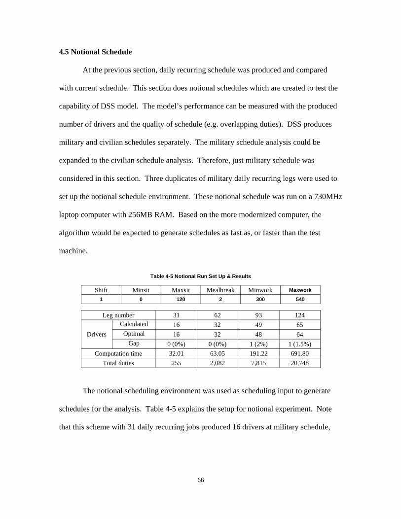
66

4.5 Notional Schedule

At the previous section, daily recurring schedule was produced and compared

with current schedule. This section does notional schedules which are created to test the

capability of DSS model. The model’s performance can be measured with the produced

number of drivers and the quality of schedule (e.g. overlapping duties). DSS produces

military and civilian schedules separately. The military schedule analysis could be

expanded to the civilian schedule analysis. Therefore, just military schedule was

considered in this section. Three duplicates of military daily recurring legs were used to

set up the notional schedule environment. These notional schedule was run on a 730MHz

laptop computer with 256MB RAM. Based on the more modernized computer, the

algorithm would be expected to generate schedules as fast as, or faster than the test

machine.

Table 4-5 Notional Run Set Up & Results

Shift Minsit Maxsit Mealbreak Minwork Maxwork

1 0 120 2 300 540

Leg number 31 62 93 124 Calculated 16 32 49 65

Optimal 16 32 48 64 Drivers Gap 0 (0%) 0 (0%) 1 (2%) 1 (1.5%)

Computation time 32.01 63.05 191.22 691.80 Total duties 255 2,082 7,815 20,748

The notional scheduling environment was used as scheduling input to generate

schedules for the analysis. Table 4-5 explains the setup for notional experiment. Note

that this scheme with 31 daily recurring jobs produced 16 drivers at military schedule,

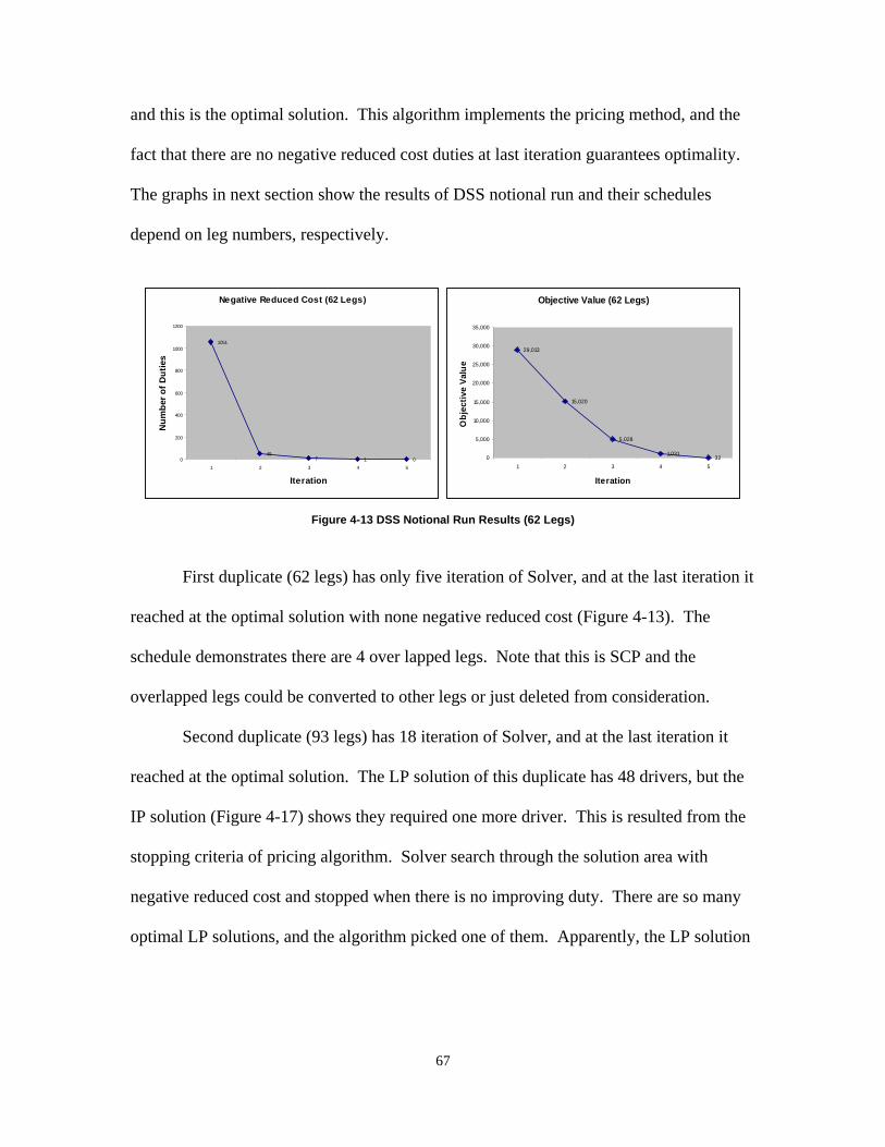
67

and this is the optimal solution. This algorithm implements the pricing method, and the

fact that there are no negative reduced cost duties at last iteration guarantees optimality.

The graphs in next section show the results of DSS notional run and their schedules

depend on leg numbers, respectively.

Negative Reduced Cost (62 Legs)

1051

497 1 00

200

400

600

800

1000

1200

1 2 3 4 5

Iteration

Num

ber o

f Dut

ies

Objective Value (62 Legs)

29,013

15,020

5,028

1,031320

5,000

10,000

15,000

20,000

25,000

30,000

35,000

1 2 3 4 5

Iteration

Obj

ectiv

e Va

lue

Figure 4-13 DSS Notional Run Results (62 Legs)

First duplicate (62 legs) has only five iteration of Solver, and at the last iteration it

reached at the optimal solution with none negative reduced cost (Figure 4-13). The

schedule demonstrates there are 4 over lapped legs. Note that this is SCP and the

overlapped legs could be converted to other legs or just deleted from consideration.

Second duplicate (93 legs) has 18 iteration of Solver, and at the last iteration it

reached at the optimal solution. The LP solution of this duplicate has 48 drivers, but the

IP solution (Figure 4-17) shows they required one more driver. This is resulted from the

stopping criteria of pricing algorithm. Solver search through the solution area with

negative reduced cost and stopped when there is no improving duty. There are so many

optimal LP solutions, and the algorithm picked one of them. Apparently, the LP solution

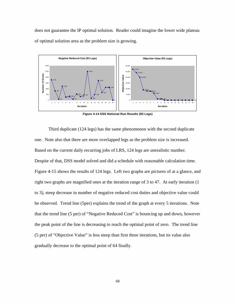
68

does not guarantee the IP optimal solution. Reader could imagine the lower wide plateau

of optimal solution area as the problem size is growing.

Negative Reduced Cost (93 Legs)

1760

810

91

1216

274 349

90

542

314451

2494

158

496

1705

658

1124 1102

00

500

1000

1500

2000

2500

3000

1 2 3 4 5 6 7 8 9 10 11 12 13 14 15 16 17 18

Iteration

Num

ber o

f Dut

ies

Objective Value (93 Legs)

27,027

24,028

20,030

9,0408,0418,041

6,043

1,0481,04748 48 48 48 48 48 48 48 480

5,000

10,000

15,000

20,000

25,000

30,000

1 2 3 4 5 6 7 8 9 10 11 12 13 14 15 16 17 18

Iteration

Obj

ectiv

e Va

lue

Figure 4-14 DSS Notional Run Results (93 Legs)

Third duplicate (124 legs) has the same phenomenon with the second duplicate

one. Note also that there are more overlapped legs as the problem size is increased.

Based on the current daily recurring jobs of LRS, 124 legs are unrealistic number.

Despite of that, DSS model solved and did a schedule with reasonable calculation time.

Figure 4-15 shows the results of 124 legs. Left two graphs are pictures of at a glance, and

right two graphs are magnified ones at the iteration range of 3 to 47. At early iteration (1

to 3), steep decrease in number of negative reduced cost duties and objective value could

be observed. Trend line (5per) explains the trend of the graph at every 5 iterations. Note

that the trend line (5 per) of “Negative Reduced Cost” is bouncing up and down, however

the peak point of the line is decreasing to reach the optimal point of zero. The trend line

(5 per) of “Objective Value” is less steep than first three iterations, but its value also

gradually decrease to the optimal point of 64 finally.

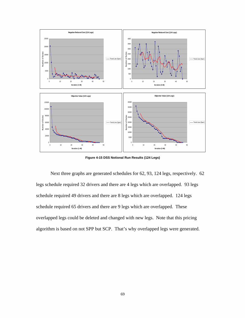
69

Negative Reduced Cost (124 Legs)

0

5000

10000

15000

20000

25000

0 10 20 30 40 50

Iteration (1-46)

Num

ber o

f Dut

ies

Trend Line (5per)

Negative Reduced Cost (124 Legs)

0

500

1000

1500

2000

2500

3000

3500

4000

0 10 20 30 40 50

Iteration (3-46)

Num

ber o

f Dut

ies

Trend Line (5per)

Objective Value (124 Legs)

0

20000

40000

60000

80000

100000

120000

0 10 20 30 40 50

Iteration (1-46)

Num

ber o

f Dut

ies

Trend Line (5per)

Objective Value (124 Legs)

0

5000

10000

15000

20000

25000

30000

35000

40000

0 10 20 30 40 50

Iteration (3-46)

Num

ber o

f Dut

ies

Trend Line (5per)

Figure 4-15 DSS Notional Run Results (124 Legs)

Next three graphs are generated schedules for 62, 93, 124 legs, respectively. 62

legs schedule required 32 drivers and there are 4 legs which are overlapped. 93 legs

schedule required 49 drivers and there are 8 legs which are overlapped. 124 legs

schedule required 65 drivers and there are 9 legs which are overlapped. These

overlapped legs could be deleted and changed with new legs. Note that this pricing

algorithm is based on not SPP but SCP. That’s why overlapped legs were generated.

70

Figure 4-16 DSS Notional Run (62 Legs)

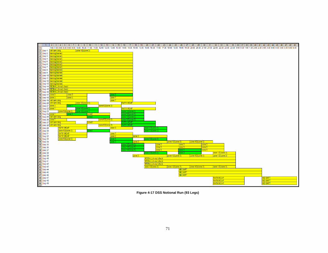
71

Figure 4-17 DSS Notional Run (93 Legs)

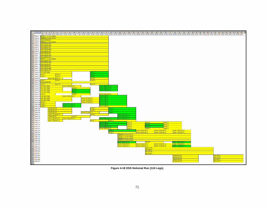
72

Figure 4-18 DSS Notional Run (124 Legs)

73

4.6 Conclusion

DSS model provides the scheduler with both a scheduling tool and analyzing tool.

Throughout the parameter analysis it was found that shift number, minimum sit time and

maximum workload parameters have more impact on the required number of drivers than

the other parameters like meal consideration and maximum sit time.

Pricing algorithm was examined with the daily recurring jobs and notional jobs

environment. It was found that DSS could handle large scale problems beyond current

LRS schedule size. The LP solution of the large problems are equal to the optimal

solution, however it requires one more driver with some IP solution.

Not only the optimal solution, but also the solution which minimize the penalty

could be found via B-Matrix. In all, the scheduling algorithm provides an initial, usable

schedule in a reasonable amount of time.

74

Chapter 5. Conclusions and Recommendations

5.1 Specific Contributions

This thesis builds an engine handling SCP associated with Excel Solver. This

model combined the concept of SCP, reduced costs, and shadow price to produce a quick

and optimal schedule. This model also could be used as an optimization tool finding a

solution in SCP with a little model modification.

This research provides LRS scheduler with a scheduling tool based on Microsoft

Excel. It is a fast approach for the scheduling problem that incorporates aspects of

resource utilization. DSS model performance with the daily recurring jobs is equal to the

optimal solution (LP). Pricing algorithm has found the optimal solution in 31 and 62

daily recurring legs and near optimal (one more driver) in 93 and 124 daily recurring legs

which are beyond the real situation number. Significant amount of the workload balance

is achieved throughout the program. Workload balance tends to transform the SCP into

SPP. This model could produce the optimal solution with current workers status. The

LRS could not always maintain enough drivers to satisfy all the requirements, and this

driver shortage leads to the undesirable results. However, the point is to minimize the

penalty value of the unsatisfied duties. This model could handle this kind of problem

with “B-Matrix”.

Various parameters’ impact on the number of required drivers was investigated.

This parameters consideration will be critical at using this model as an analysis tool. The

scheduler may figure out the expected number of drivers with future amount of customers

75

or legs. This model will provide more advanced insights in future work environment

with policy maker such like LRS commander. In brief, DSS model will answer the

following kinds of questions: 1) “How many drivers do we need with X amount of

customers?” 2) “Which parameter set up is better than current setup? Better means less

drivers, less AvgWL, and fully accomplishment of the total legs simultaneously.”

5.2 Recommendations for Future Work

First, this model does not produce full schedule which include the drivers roster,

distribute the duties to the real workers and examine a long term workload. This

procedure will provide more practical outcomes with the LRS scheduler.

Second, the future research could handle the vehicle routing problem.

Throughout this research, vehicle routing within each Zone is fixed by the LRS. The

researcher can examine the routes and find more efficient way to execute the mission

than current way.

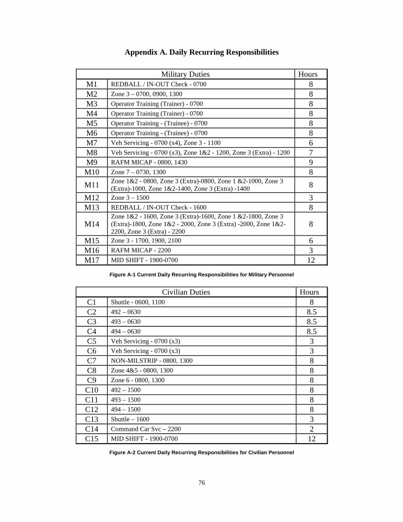
76

Appendix A. Daily Recurring Responsibilities

Military Duties Hours

M1 REDBALL / IN-OUT Check - 0700 8 M2 Zone 3 – 0700, 0900, 1300 8 M3 Operator Training (Trainer) - 0700 8 M4 Operator Training (Trainer) - 0700 8 M5 Operator Training - (Trainee) - 0700 8 M6 Operator Training - (Trainee) - 0700 8 M7 Veh Servicing - 0700 (x4), Zone 3 - 1100 6 M8 Veh Servicing - 0700 (x3), Zone 1&2 - 1200, Zone 3 (Extra) - 1200 7 M9 RAFM MICAP - 0800, 1430 9 M10 Zone 7 – 0730, 1300 8 M11 Zone 1&2 - 0800, Zone 3 (Extra)-0800, Zone 1 &2-1000, Zone 3

(Extra)-1000, Zone 1&2-1400, Zone 3 (Extra) -1400 8 M12 Zone 3 – 1500 3 M13 REDBALL / IN-OUT Check - 1600 8

M14 Zone 1&2 - 1600, Zone 3 (Extra)-1600, Zone 1 &2-1800, Zone 3 (Extra)-1800, Zone 1&2 - 2000, Zone 3 (Extra) -2000, Zone 1&2-2200, Zone 3 (Extra) - 2200

8

M15 Zone 3 - 1700, 1900, 2100 6 M16 RAFM MICAP - 2200 3 M17 MID SHIFT - 1900-0700 12

Figure A-1 Current Daily Recurring Responsibilities for Military Personnel

Civilian Duties Hours

C1 Shuttle - 0600, 1100 8 C2 492 – 0630 8.5 C3 493 – 0630 8.5 C4 494 – 0630 8.5 C5 Veh Servicing - 0700 (x3) 3 C6 Veh Servicing - 0700 (x3) 3 C7 NON-MILSTRIP - 0800, 1300 8 C8 Zone 4&5 - 0800, 1300 8 C9 Zone 6 - 0800, 1300 8 C10 492 – 1500 8 C11 493 – 1500 8 C12 494 – 1500 8 C13 Shuttle – 1600 3 C14 Command Car Svc – 2200 2 C15 MID SHIFT - 1900-0700 12

Figure A-2 Current Daily Recurring Responsibilities for Civilian Personnel

77

Bibliography

1. E. H. L. Aarts, J. K. Lenstra (eds.). Local Search in Combinatorial Optimization. Chichester: John Wiley & Sons, 1997.

2. Albright, Christian S. VBA for Modelers, Pacific Grove, Wadsworth Group, 2001. 3. Balas, E., M. C. Carrera. “A dynamic subgradient-based branch and bound

procedure for set covering,” Oper. Res. 44: 875-890 (1996). 4. Balas, E., A. Ho. “Set covering algorithms using cutting planes, heuristics and

subgradient optimization: a computational study,” Math. Programming Study 12: 37-60 (1980).

5. Bazaraa, M. S.,John J. Jarvis, Hanif D. Sherali, Linear Programming and Network Flows. New York: Wiley & Sons, 1990.

6. Beasley, J. E. “An algorithm for set covering problems,” European J. Oper. Res. 31: 85-93 (1987).

7. Beasley, J. E. “A Lagrangian heuristic for set covering problems,” Naval Res. Logistics 37: 151-164 (1990).

8. Beasley, J. E., P. C. Chu. “A genetic algorithm for the set covering problem,” European J. Oper. Res. 94: 392-404 (1996).

9. Beasley, J. E., K. Jörnsten. “Enhancing an algorithm for set covering problems,” European J. Oper. Res. 58: 293-300 (1992).

10. Bodin, L., B. Golden, A. Assad, and M. Ball, “Routing and scheduling of vehicles and crews: The state of art,” Comput. Oper. Res., 10(2): 63-211 (1983).

11. Carlton, William B. A Tabu search to the General Vehicle Routing Problem. Ph.D. dissertation. University of Texas, Austin TX, (1995).

12. Ceria, S., P. Nobili, A. Sassano. “A Larangian-based heuristic for large-scale set covering problems,” Technical Report R.406, IASI-CNR, Roma (1995), To appear in Math. Programming.

13. Combs, Todd E. A Combined Adaptive Tabu Search and Set Partitioning Approach for the Crew Scheduling Problem with an Air Tanker Crew Application. Ph.D. dissertation. Air Force Institute of Technology, Wright-Patterson AFB OH, (2002).

14. Evren, Fuat. SSS: A Knowledge-Based Approach to Resource Scheduling in an F-16 Fighter Training Unit, Term Project, Middle East Technical University, 1999.

15. Fisher, M. L., P. Kedia. “Optimal solutions of set covering/partitioning problems using dual heuristics,” Management Sci. 36: 674-688 (1990).

16. Freling, Richard and others. “Models and Algorithms for Integration of Vehicle and Crew Scheduling,” Journal of Scheduling, 6: 63-85 (2003).

17. Gershkoff, I. “Optimizing Flight Crew Schedules,” Interfaces, 19(4): 29-43 (1989). 18. Kirkpatrick, S., Gerlatt, C. D. Jr., and Vecchi, M.P., “Optimization by Simulated

Annealing,” Science 220: 671-680 (1983). 19. Lawer, E.L.,J.K. Lenstra, A.H.G. Rinnooy Kan, and D.B. Shmoys. The Traveling

Salesman Problem. A Guided Tour of Combinatorial Optimization. John Wiley & Sons Ltd, 1985.

78

20. Lorena, L. A. N., F. B. Lopes. “A surrogate heuristic for set covering problems,” European J. Oper. Res. 79: 138-150 (1994).

21. Nobili, P., A. Sassano. “A separation routine for the set covering polytope,” E. Balas, G. Cornuejols, R. Kannan, eds. “Integer Programming and Combinatorial Optimization,” Proceedings of the 2nd IPCO Conference, Carengie Mellon University Press, Pittsburgh, PA (1992).

22. Nguyen, Cuong T. An Interactive Decision Support System For Scheduling Fighter Pilot Training. MS thesis, AFIT/GOR/ENS/02-12. School of Engineering and Management, Air Force Institute of Technology (AU), Wright-Patterson AFB OH, 2002.

23. Pinedo, Michael. Scheduling theory, Algorithms, and Systems, New Jersey: Prentice-Hall, 2002.

24. Wedelin, D. “An algorithm for large scale 0-1 integer programming with application to airline crew scheduling,” Ann. Oper. Res. 57: 283-301 (1995).

25. Winston, Wayne. L. Operations Research Applications and Algorithms, Belmont: Thomson, 2004.

79

Vita

Captain Young-ho Cha graduated from Tae-gu public High School in Tae-gu,

Korea. He entered undergraduate studies at the Korea Military Academy (KMA) where

he graduated with a Bachelor of Science Degree in Weapon Engineering and received a

regular commission in March 1996.

He successfully performed various assignments all around Korea for nine years.

In August 2003, he entered the Graduate School of Engineering and Management, Air

Force Institute of Technology. Upon graduation, he will be assigned to the Combined

Forces Command.

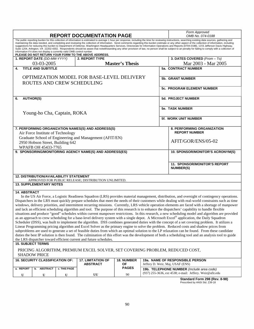
90

REPORT DOCUMENTATION PAGE Form Approved OMB No. 074-0188

The public reporting burden for this collection of information is estimated to average 1 hour per response, including the time for reviewing instructions, searching existing data sources, gathering and maintaining the data needed, and completing and reviewing the collection of information. Send comments regarding this burden estimate or any other aspect of the collection of information, including suggestions for reducing this burden to Department of Defense, Washington Headquarters Services, Directorate for Information Operations and Reports (0704-0188), 1215 Jefferson Davis Highway, Suite 1204, Arlington, VA 22202-4302. Respondents should be aware that notwithstanding any other provision of law, no person shall be subject to an penalty for failing to comply with a collection of information if it does not display a currently valid OMB control number. PLEASE DO NOT RETURN YOUR FORM TO THE ABOVE ADDRESS. 1. REPORT DATE (DD-MM-YYYY)

03-03-2005 2. REPORT TYPE

Master’s Thesis 3. DATES COVERED (From – To)

Mar 2003 - Mar 2005 5a. CONTRACT NUMBER

5b. GRANT NUMBER

4. TITLE AND SUBTITLE

OPTIMIZATION MODEL FOR BASE-LEVEL DELIVERY ROUTES AND CREW SCHEDULING

5c. PROGRAM ELEMENT NUMBER

5d. PROJECT NUMBER 5e. TASK NUMBER

6. AUTHOR(S) Young-ho Cha, Captain, ROKA

5f. WORK UNIT NUMBER

7. PERFORMING ORGANIZATION NAMES(S) AND ADDRESS(S) Air Force Institute of Technology Graduate School of Engineering and Management (AFIT/EN) 2950 Hobson Street, Building 642 WPAFB OH 45433-7765

8. PERFORMING ORGANIZATION REPORT NUMBER AFIT/GOR/ENS/05-02

10. SPONSOR/MONITOR’S ACRONYM(S) 9. SPONSORING/MONITORING AGENCY NAME(S) AND ADDRESS(ES)

11. SPONSOR/MONITOR’S REPORT NUMBER(S)

12. DISTRIBUTION/AVAILABILITY STATEMENT APPROVED FOR PUBLIC RELEASE; DISTRIBUTION UNLIMITED. 13. SUPPLEMENTARY NOTES 14. ABSTRACT In the US Air Force, a Logistic Readiness Squadron (LRS) provides material management, distribution, and oversight of contingency operations. Dispatchers in the LRS must quickly prepare schedules that meet the needs of their customers while dealing with real-world constraints such as time windows, delivery priorities, and intermittent recurring missions. Currently, LRS vehicle operation elements are faced with a shortage of manpower and lack an efficient scheduling algorithm and tool. The purpose of this research is to enhance the dispatchers’ capability to handle flexible situations and produce “good” schedules within current manpower restrictions. In this research, a new scheduling model and algorithm are provided as an approach to crew scheduling for a base-level delivery system with a single depot. A Microsoft Excel® application, the Daily Squadron Scheduler (DSS), was built to implement the algorithm. DSS combines generated duties with the concept of a set covering problem. It utilizes a Linear Programming pricing algorithm and Excel Solver as the primary engine to solve the problem. Reduced costs and shadow prices from subproblems are used to generate a set of feasible duties from which an optimal solution to the LP relaxation can be found. From these candidate duties the best IP solution is then found. The culmination of this effort was the development of both a scheduling tool and an analysis tool to guide the LRS dispatcher toward efficient current and future schedules. 15. SUBJECT TERMS

PRICING ALGORITHM, PREMIUM EXCEL SOLVER, SET COVERING PROBLEM, REDUCED COST, SHADOW PRICE

16. SECURITY CLASSIFICATION OF: 19a. NAME OF RESPONSIBLE PERSON Jeffery D. Weir, Maj, USAF (ENS)

a. REPORT

U

b. ABSTRACT

U

c. THIS PAGE

U

17. LIMITATION OF ABSTRACT

UU

18. NUMBER OF PAGES

90 19b. TELEPHONE NUMBER (Include area code) (937) 255-3636, ext 4538; e-mail: Jeffery. Weir@afit.edu

Standard Form 298 (Rev. 8-98) Prescribed by ANSI Std. Z39-18