Optimization methods on Riemannian manifolds and their

application to shape space

Wolfgang Ring Benedikt Wirth

Abstract

We extend the scope of analysis for linesearch optimization algorithms on (possibly infinite-dimensional) Riemannian manifolds to the convergence analysis of the BFGS quasi-Newton schemeand the Fletcher–Reeves conjugate gradient iteration. Numerical implementations for exemplaryproblems in shape spaces show the practical applicability of these methods.

1 Introduction

There are a number of problems that can be expressed as a minimization of a function f :M→ R overa smooth Riemannian manifold M. Applications range from linear algebra (e. g. principal componentanalysis or singular value decomposition, [1, 11]) to the analysis of shape spaces (e. g. computation ofshape geodesics, [24]), see also the references in [3].

If the manifold M can be embedded in a higher-dimensional space or if it is defined via equalityconstraints, then there is the option to employ the very advanced tools of constrained optimization(see [16] for an introduction). Often, however, such an embedding is not at hand, and one has toresort to optimization methods designed for Riemannian manifolds. Even if an embedding is known,one might hope that a Riemannian optimization method performs more efficiently since it exploits theunderlying geometric structure of the manifold. For this purpose, various methods have been devised,from simple gradient descent on manifolds [25] to sophisticated trust region methods [5]. The aim ofthis article is to extend the scope of analysis for these methods, concentrating on linesearch methods.In particular, we will consider the convergence of BFGS quasi-Newton methods and Fletcher–Reevesnonlinear conjugate gradient iterations on (possibly infinite-dimensional) manifolds, thereby filling a gapin the existing analysis. Furthermore, we apply the proposed methods to exemplary problems, showingtheir applicability to manifolds of practical interest such as shape spaces.

Early attempts to adapt standard optimization methods to problems on manifolds were presentedby Gabay [9] who introduced a steepest descent, a Newton, and a quasi-Newton algorithm, also statingtheir global and local convergence properties (however, without giving details of the analysis for thequasi-Newton case). Udriste [23] also stated a steepest descent and a Newton algorithm on Riemannianmanifolds and proved (linear) convergence of the former under the assumption of exact linesearch. Fairlyrecently, Yang took up these methods and analysed convergence and convergence rate of steepest descentand Newton’s method for Armijo step-size control [25].

In comparison to standard linesearch methods in vector spaces, the above approaches all substitutethe linear step in the search direction by a step along a geodesic. However, geodesics may be difficult toobtain. In alternative approaches, the geodesics are thus often replaced by more general paths, based onso-called retractions (a retraction Rx is a mapping from the tangent space TxM to the manifold M atx onto M). For example, Huper and Trumpf find quadratic convergence for Newton’s method withoutstep-size control [11], even if the Hessian is computed for a different retraction than the one defining thepath along which the Newton step is taken. In the sequel, more advanced trust region Newton methodshave been developed and analysed in a series of papers [6, 1, 5]. The analysis requires some type ofuniform Lipschitz continuity for the gradient and the Hessian of the concatenations f ◦ Rx, which wewill also make use of. The global and local convergence analysis of gradient descent, Newton’s method,and trust region methods on manifolds with general retractions is summarized in [2].

In [2], the authors also present a way to implement a quasi-Newton as well as a nonlinear conjugategradient iteration, however, without analysis. Riemannian BFGS quasi-Newton methods, which gener-alize Gabay’s original approach, have been devised in [18]. Like the above schemes, they do not rely on

1

geodesics but allow more general retractions. Furthermore, the vector transport between the tangentspaces TxkM and Txk+1

M at two subsequent iterates (which is needed for the BFGS update of the Hes-sian approximation) is no longer restricted to parallel transport. A similar approach is taken in [7], wherea specific, non-parallel vector transport is considered for a linear algebra application. A correspondingglobal convergence analysis of a quasi-Newton scheme has been performed by Ji [12]. However, to obtaina superlinear convergence rate, specific conditions on the compatibility between the vector transportsand the retractions are required (cf. section 3.1) which are not imposed (at least explicitly) in the abovework.

In this paper, we pursue several objectives. First, we extend the convergence analysis of standardRiemannian optimization methods (such as steepest descent and Newton’s method) to the case of opti-mization on infinite-dimensional manifolds. Second, we analyze the convergence rate of the RiemannianBFGS quasi-Newton method as well as the convergence of a Riemannian Fletcher–Reeves conjugategradient iteration (as two representative higher order gradient-based optimization methods), which tothe authors’ knowledge has not been attempted before (neither in the finite- nor the infinite-dimensionalcase). The analysis is performed in the unifying framework of step-size controlled linesearch methods,which allows for rather streamlined proofs. Finally, we demonstrate the feasibility of these Riemannianoptimization methods by applying them to problems in state-of-the-art shape spaces.

The outline of this article is as follows. Section 2 summarizes the required basic notions. Section 3 thenintroduces linesearch optimization methods on Riemannian manifolds, following the standard procedurefor finite-dimensional vector spaces [16, 17] and giving the analysis of basic steepest descent and Newton’smethod as a prerequisite for the ensuing analysis of the BFGS scheme in section 3.1 and the nonlinearCG iteration in section 3.2. Finally, numerical examples on shape spaces are provided in section 4.

2 Notations

Let M denote a geodesically complete (finite- or infinite-dimensional) Riemannian manifold. In partic-ular, we assumeM to be locally homeomorphic to some separable Hilbert space H [14, Sec. 1.1], that is,for each x ∈ M there is some neighborhood x ∈ Ux ⊂M and a homeomorphism φx from Ux into someopen subset of H. Let C∞(M) denote the vector space of smooth real functions onM (in the sense thatfor any f ∈ C∞(M) and any chart (Ux, φx), f ◦ φ−1x is smooth). For any smooth curve γ : [0, 1] →Mwe define the tangent vector to γ at t0 ∈ (0, 1) as the linear operator γ(t0) : C∞(M)→ R such that

γ(t0)f =

(d

dtf ◦ γ

)(t0) ∀f ∈ C∞(M) .

The tangent space TxM to M in x ∈ M is the set of tangent vectors γ(t0) to all smooth curvesγ : [0, 1] → M with γ(t0) = x. It is a vector space, and it is equipped with an inner product gx(·, ·) :TxM× TxM→ R, the so-called Riemannian metric, which smoothly depends on x. The correspondinginduced norm will be denoted ‖·‖x, and we will employ the same notation for the associated dual norm.

Let V(M) denote the set of smooth tangent vector fields on M, then we define a connection ∇ :V(M)× V(M)→ V(M) as a map such that

∇fX+gY Z = f∇XZ + g∇Y Z ∀X,Y, Z ∈ V(M) and f, g ∈ C∞(M) ,

∇Z(aX + bY ) = a∇ZX + b∇ZY ∀X,Y, Z ∈ V(M) and a, b ∈ R ,∇Z(fX) = (Zf)X + f∇ZX ∀X,Z ∈ V(M) and f ∈ C∞(M) .

In particular, we will consider the Levi-Civita connection, which additionally satisfies the properties ofabsence of torsion and preservation of the metric,

[X,Y ] = ∇XY −∇YX ∀X,Y ∈ V(M) ,

Xg(Y,Z) = g(∇XY,Z) + g(Y,∇XZ) ∀X,Y, Z ∈ V(M) ,

where [X,Y ] = XY − Y X denotes the Lie bracket and g(X,Y ) :M3 x 7→ gx(X,Y ).Any connection is paired with a notion of parallel transport. Given a smooth curve γ : [0, 1] →M,

the initial value problem∇γ(t)v = 0, v(0) = v0

2

defines a way of transporting a vector v0 ∈ Tγ(0)M to a vector v(t) ∈ Tγ(t)M. For the Levi-Civitaconnection considered here this implies constancy of the inner product gγ(t)(v(t), w(t)) for any twovectors v(t), w(t), transported parallel along γ. For x = γ(0), y = γ(t), we will denote the parallel

transport of v(0) ∈ TxM to v(t) ∈ TyM by v(t) = TPγx,yv(0) (if there is more than one t with y = γ(t),

the correct interpretation will become clear from the context). As detailed further below, TPγx,y can be

interpreted as the derivative of a specific mapping Pγ : TxM→M.We assume that any two points x, y ∈ M can be connected by a shortest curve γ : [0, 1] →M with

x = γ(0), y = γ(1), where the curve length is measured as

L[γ] =

∫ 1

0

√gγ(t)(γ(t), γ(t)) dt .

Such a curve is denoted a geodesic, and the length of geodesics induces a metric distance on M,

dist(x, y) = minγ:[0,1]→M

γ(0)=x,γ(1)=y

L[γ] .

If the geodesic γ connecting x and y is unique, then γ(0) ∈ TxM is denoted the logarithmic map ofy with respect to x, logx y = γ(0). It satisfies dist(x, y) = ‖logx y‖x. Geodesics can be computed viathe zero acceleration condition ∇γ(t)γ(t) = 0. The exponential map expx : TxM→M, v 7→ expx v, isdefined as expx v = γ(1), where γ solves the above ordinary differential equation with initial conditionsγ(0) = x, γ(0) = v. It is a diffeomorphism of a neighborhood of 0 ∈ TxM into a neighborhood of x ∈Mwith inverse logx. We shall denote the geodesic between x and y by γ[x; y], assuming that it is unique.

The exponential map expx obviously provides a (local) parametrization ofM via TxM. We will alsoconsider more general parameterizations, so-called retractions. Given x ∈ M, a retraction is a smoothmapping Rx : TxM → M with Rx(0) = x and DRx(0) = idTxM, where DRx denotes the derivativeof Rx. The inverse function theorem then implies that Rx is a local homeomorphism. Besides expx,there are various possibilities to define retractions. For example, consider a geodesic γ : R → M withγ(0) = x, parameterized by arc length, and define the retraction

Pγ : TxM→M , v 7→ exppγ(v)

(TPγx,pγ(v)

[v − πγ(v)]),

where pγ(v) = expx(πγ(v)) and πγ denotes the orthogonal projection onto span{γ(0)}. This retractioncorresponds to running along the geodesic γ according to the component of v parallel to γ(0) and thenfollowing a new geodesic into the direction of the parallel transported component of v orthogonal to γ(0).

We will later have to consider the transport of a vector from one tangent space TxM into anotherone TyM, that is, we will consider isomorphisms Tx,y : TxM→ TyM. We are particularly interested in

operators TRxx,y which represent the derivative DRx(v) of a retraction Rx at v ∈ TxM with Rx(v) = y(where in case of multiple v with Rx(v) = y it will be clear from the context which v is meant). In that

sense, the parallel transport TPγx,y along a geodesic γ connecting x and y belongs to the retraction Pγ .

Another possible vector transport is defined by the variation of the exponential map, evaluated at therepresentative of y in TxM,

T expxx,y = D expx(logx y) ,

which maps each v0 ∈ TxM onto the tangent vector γ(0) to the curve γ : t 7→ expx(logx y + tv0). Also

the adjoints (TPγy,x)∗, (T

expyy,x )∗ (defined by gy(v, T ∗y,xw) = gx(Ty,xv, w) ∀v ∈ TyM, w ∈ TxM) or inverses

(TPγy,x)−1, (T

expyy,x )−1 can be considered for vector transport Tx,y. Note that T

Pγx,y is an isometry with

TPγx,y = (T

Pγy,x)∗ = (T

Pγy,x)−1, where γ is the geodesic connecting x with y and γ(·) = γ(−·). Furthermore,

logx y is transported onto the same vector Tx,y logx y = γ(1) by TPγx,y, T

expxx,y and their adjoints and

inverses.Given a smooth function f :M→ R, we define its (Frechet-)derivative Df(x) at a point x ∈ M as

an element of the dual space to TxM via Df(x)v = vf . The Riesz representation theorem then impliesthe existence of a ∇f(x) ∈ TxM such that Df(x)v = gx(∇f(x), v) for all v ∈ TxM, which we denotethe gradient of f at x. On TxM, define

fRx = f ◦Rx

3

for a retraction Rx. Due to DRx(0) = id we have DfRx(0) = Df(x). Furthermore, fRx = fRy ◦R−1y ◦Rxwhere R−1y exists and thus for y = Rx(v),

DfRx(v) = DfRy (0)DRx(v) = Df(y)TRxx,y , ∇fRx(v) = (TRxx,y )∗∇f(y) .

We define the Hessian D2f(x) of a smooth f at x as the symmetric bilinear form D2f(x) : TxM×TxM→ R, (v, w) 7→ gx(∇v∇f(x), w), which is equivalent to D2f(x) = D2fexpx(0). By ∇2f(x) : TxM→TxM we denote the linear operator mapping v ∈ TxM onto the Riesz representation of D2f(x)(v, ·).Note that if M is embedded into a vector space X and f = f |M for a smooth f : X → R, we usually

have D2f(x) 6= D2f(x)|TxM×TxM (which is easily seen from the example X = Rn, f(x) = ‖x‖2X ,M = {x ∈ X : ‖x‖X = 1}). For a smooth retraction Rx we do not necessarily have D2fRx(0) = D2f(x),however, this holds at stationary points of f [1, 2].

Let T n(TxM) denote the vector space of n-linear forms T : (TxM)n → R together with the norm

‖T‖x = supv1,...,vn∈TxMT (v1,...,vn)‖v1‖x...‖vn‖x . We call a function g : M →

⋃x∈M T n(TxM), x 7→ g(x) ∈

T n(TxM), (Lipschitz) continuous at x ∈M if x 7→ g(x)◦(TPγ[x;x]x,x )n ∈ T n(TxM) is (Lipschitz) continuous

at x (with Lipschitz constant lim supx→x

∥∥∥g(x) ◦ (TPγ[x;x]x,x )n − g(x)

∥∥∥x/dist(x, x)). Here, γ[x;x] denotes

the shortest geodesic, which is unique in the neighborhood of x. (Lipschitz) continuity on U ⊂M means(Lipschitz) continuity at every x ∈ U (with uniform Lipschitz constant). A function f :M→ R is calledn times (Lipschitz) continuously differentiable, if Dlf :M→

⋃x∈M T l(TxM) is (Lipschitz) continuous

for 0 ≤ l ≤ n.

3 Iterative minimization via geodesic linesearch methods

In classical optimization on vector spaces, linesearch methods are widely used. They are based onupdating the iterate by choosing a search direction and then adding a multiple of this direction to theold iterate. Adding a multiple of the search direction obviously requires the structure of a vector spaceand is not possible on general manifolds. The natural extension to manifolds is to follow the searchdirection along a path. We will consider iterative algorithms of the following generic form.

Algorithm 1 (Linesearch minimization on manifolds).

Input: f :M→ R, x0 ∈M, k = 0repeat

choose a descent direction pk ∈ TxkMchoose a retraction Rxk : TxkM→Mchoose a step length αk ∈ Rset xk+1 = Rxk(αkpk)k ← k + 1

until xk+1 sufficiently minimizes f

Here, a descent direction denotes a direction pk with Df(xk)pk < 0. This property ensures that theobjective function f indeed decreases along the search direction.

For the choice of the step length, various approaches are possible. In general, the chosen αk has tofulfill a certain quality requirement. We will here concentrate on the so-called Wolfe conditions, that is,for a given descent direction p ∈ TxM, the chosen step length α has to satisfy

f(Rx(αp)) ≤ f(x) + c1αDf(x)p , (1a)

Df(Rx(αp))TRxx,Rx(αp)p ≥ c2Df(x)p , (1b)

where 0 < c1 < c2 < 1. Note that both conditions can be rewritten as fRx(αp) ≤ fRx(0) + c1αDfRx(0)pand DfRx(αp)p ≥ c2DfRx(0)p, the classical Wolfe conditions for minimization of fRx . If the secondcondition is replaced by

|Df(Rx(αp))TRxx,Rx(αp)p| ≤ −c2Df(x)p , (2)

we obtain the so-called strong Wolfe conditions. Most optimization algorithms also work properly if justthe so-called Armijo condition (1a) is satisfied. In fact, the stronger Wolfe conditions are only neededfor the later analysis of a quasi-Newton scheme. Given a descent direction p, a feasible step length canalways be found.

4

Proposition 1 (Feasible step length, e. g. [16, Lem. 3.1]). Let x ∈ M, p ∈ TxM be a descent directionand fRx : span{p} → R continuously differentiable. Then there exists α > 0 satisfying (1) and (2).

Proof. Rewriting the Wolfe conditions as fRx(αp) ≤ fRx(0)+c1αDfRx(0)p and DfRx(αp)p ≥ c2DfRx(0)p(|DfRx(αp)p| ≤ −c2DfRx(0)p, respectively), the standard argument for Wolfe conditions in vector spacescan be applied.

Besides the quality of the step length, the convergence of linesearch algorithms naturally depends onthe quality of the search direction. Let us introduce the angle θk between the search direction pk andthe negative gradient −∇f(xk),

cos θk =−Df(xk)pk

‖Df(xk)‖xk ‖pk‖xk.

There is a classical link between the convergence of an algorithm and the quality of its search direction.

Theorem 2 (Zoutendijk’s theorem). Given f : M → R bounded below and differentiable, assume theαk in Algorithm 1 to satisfy (1). If the fRxk are Lipschitz continuously differentiable on span{pk} withuniform Lipschitz constant L, then ∑

k∈Ncos2 θk ‖Df(xk)‖2xk <∞ .

Proof. The proof for optimization on vector spaces also applies here: Lipschitz continuity and (1b) imply

αkL ‖pk‖2xk ≥ (DfRxk (αkpk)−DfRxk (0))pk ≥ (c2 − 1)Df(xk)pk ,

from which we obtain αk ≥ (c2 − 1)Df(xk)pk/(L ‖pk‖2xk). Then (1a) implies

f(xk+1) ≤ f(xk)− c11− c2L

cos2 θk ‖Df(xk)‖2xk

so that the result follows from the boundedness of f by summing over all k.

Corollary 3 (Convergence of generalized steepest descent). Let the search direction in Algorithm 1 bethe solution to Bk(pk, v) = −Df(xk)v ∀v ∈ TxkM, where the Bk are uniformly coercive and boundedbilinear forms on TxkM (the case Bk(·, ·) = gxk(·, ·) yields the steepest descent direction). Under theconditions of Theorem 2, ‖Df(xk)‖xk → 0.

Proof. Obviously, cos θk = Bk(pk,pk)‖Bk(pk,·)‖xk‖pk‖xk

is uniformly bounded above zero so that the convergence

follows from Zoutendijk’s theorem.

For continuous Df , the previous corollary implies that any limit point x∗ of the sequence xk is astationary point of f . Hence, on finite-dimensional manifolds, if {x ∈M : f(x) ≤ f(x0)} is bounded, xkcan be decomposed into subsequences each of which converges against a stationary point. On infinite-dimensional manifolds, where only a weak convergence of subsequences can be expected, this is not truein general (which is not surprising given that not even existence of stationary points is granted withoutstronger conditions on f such as sequential weak lower semi-continuity). Moreover, the limit points maybe non-unique. However, in the case of (locally) strictly convex functions we have (local) convergenceagainst the unique minimizer by the following classical estimate.

Proposition 4. Let U ⊂ M be a geodesically star-convex neighborhood around x∗ ∈ M (i. e. for anyx ∈ U the shortest geodesics from x∗ to x lie inside U), and define

V (U) = {v ∈ exp−1x∗ (U) : ‖v‖x∗ ≤ ‖w‖x∗ ∀w ∈ exp−1x∗ (expx∗(v))} .

Let f be twice differentiable on U with x∗ being a stationary point. If D2fexpx∗ is uniformly coercive onV (U) ⊂ Tx∗M, then there exists m > 0 such that for all x ∈ U ,

dist(x, x∗) ≤ 1

m‖Df(x)‖x .

5

Proof. By hypothesis, there is m > 0 with D2fexpx∗ (x)(v, v) ≥ m ‖v‖2x∗ for all x ∈ exp−1x∗ (U), v ∈ Tx∗M.

Thus, for v = logx∗ x we have ‖Df(x)‖x ≥|Df(x) logx x

∗|‖logx x∗‖x

=|Dfexpx∗ (v)v|‖v‖x∗

=|∫ 1

0D2fexpx∗ (tv)(v,v) dt|

‖v‖x∗≥

m ‖v‖x = mdist(x, x∗). (Note that coercivity along γ[x;x∗] would actually suffice.)

Hence, if f is smooth with Df(x∗) = 0 and D2f(x∗) = D2fexpx∗ (0) coercive (so that there existsa neighborhood U ⊂ M of x∗ such that D2fexpx∗ is uniformly coercive on V (U)), then by the aboveproposition and Corollary 3 we thus have xk → x∗ if {x ∈M : f(x) ≤ f(x0)} ⊂ U .

Remark 1. Note the difference between steepest descent and an approximation of the so-called gradientflow, the solution to the ODE

dx

dt= −∇f(x) .

While the gradient flow aims at a smooth curve along which the direction at each point is the steepestdescent direction, the steepest descent linesearch tries to move into a fixed direction as long as possibleand only changes its direction to be the one of steepest descent if the old direction does no longer yieldsufficient decrease. Therefore, the steepest descent typically takes longer steps in one direction.

Remark 2. The condition on fRxk in Theorems 1 and 2 may be untangled into conditions on f and Rxk .

For example, one might require f to be Lipschitz continuously differentiable and TRxkxk,xk+1 |span{pk} to be

uniformly bounded, which is the case for Rxk = expxk or Rxk = Pγ[xk;xk+1], for example.

As a method with only linear convergence, steepest descent requires many iterations. Improvementcan be obtained by choosing in each iteration the Newton direction pNk as search direction, that is, thesolution to

D2fRxk (0)(pNk , v) = −Df(xk)v ∀v ∈ TxkM . (3)

Note that the Newton direction is obtained with regard to the retraction Rxk . The fact that D2fRx∗ (0) =D2f(x∗) at a stationary point x∗ and the later result that the Hessian only needs to be approximated(Proposition 8) suggests that D2f(xk) or a different approximation could be used as well to obtain fastconvergence. In contrast to steepest descent, Newton’s method is invariant with respect to a rescalingof f and in the limit allows a constant step size and quadratic convergence as shown in the followingsequence of propositions which can be transferred from standard results (e. g. [16, Sec. 3.3]).

Proposition 5 (Newton step length). Let f be twice differentiable and D2fRx(0) continuous in x.Consider Algorithm 1 and assume the αk to satisfy (1) with c1 ≤ 1

2 and the pk to satisfy

limk→∞

∥∥∥Df(xk) + D2fRxk (0)(pk, ·)∥∥∥xk

‖pk‖xk= 0 . (4)

Furthermore, let the fRxk be twice Lipschitz continuously differentiable on span{pk} with uniform Lip-

schitz constant L. If x∗ with Df(x∗) = 0 and D2f(x∗) bounded and coercive is a limit point of xk sothat xk →k∈I x

∗ for some I ⊂ N, then αk = 1 would also satisfy (1) (independent of whether αk = 1 isactually chosen) for sufficiently large k ∈ I.

Proof. Let m > 0 be the lowest eigenvalue belonging to D2f(x∗) = D2fRx∗ (0). The continuity of the

second derivative implies the uniform coercivity D2fRxk(0)(v, v) ≥ m2 ‖v‖

2xk

for all k ∈ I sufficiently

large. From D2fRxk (0)(pk − pNk , ·) = Df(xk) + D2fRxk (0)(pk, ·) we then obtain pk − pNk = o(‖pk‖xk).

Furthermore, condition (4) implies limk→∞ |Df(xk)pk + D2fRxk(0)(pk, pk)|/ ‖pk‖2xk = 0 and thus

0 = lim supk→∞

Df(xk)pk

‖pk‖2xk+

D2fRxk(0)(pk, pk)

‖pk‖2xk≥ lim supk→∞,k∈I

Df(xk)pk

‖pk‖2xk+m

2⇒ −Df(xk)pk/ ‖pk‖2xk ≥

m

4

(5)for k ∈ I sufficiently large. Due to ‖Df(xk)‖xk →k∈I 0 we deduce ‖pk‖xk →k∈I 0.

6

By Taylor’s theorem, fRxk(pk)=fRxk(0)+DfRxk(0)pk+12D2fRxk(qk)(pk, pk) for some qk∈[0, pk] so that

fRxk(pk)− f(xk)− 1

2Df(xk)pk =

1

2(Df(xk)pk + D2fRxk(qk)(pk, pk))

=1

2

[ (Df(xk)pk + D2fRxk(0)(pNk , pk)

)+ D2fRxk(0)(pk − pNk , pk)

+(

D2fRxk(qk)−D2fRxk(0))

(pk, pk)]

≤ o(‖pk‖2xk)

which implies feasibility of αk = 1 with respect to (1a) for k ∈ I sufficiently large. Also,

|DfRxk(pk)pk| =∣∣∣∣Df(xk)pk + D2fRxk(0)(pk, pk) +

∫ 1

0

(D2fRxk(tpk)−D2fRxk(0)

)(pk, pk) dt

∣∣∣∣ = o(‖pk‖2xk)

which together with (5) implies DfRxk(pk)pk ≥ c2Df(xk)pk for sufficiently large k ∈ I, that is, (1b) forαk = 1.

Lemma 6. Let U ⊂M be open and retractions Rx : TxM→M, x ∈ U , have equicontinuous derivativesat x in the sense

∀ε > 0∃δ > 0∀x ∈ U : ‖v‖x < δ ⇒∥∥∥TPγ[x;Rx(v)]

x,Rx(v)DRx(0)−DRx(v)

∥∥∥ < ε .

Then for any ε > 0 there is an ε′ > 0 such that for all x ∈ U and v, w ∈ TxM with ‖v‖x , ‖w‖x < ε′,

(1− ε) ‖w − v‖x ≤ dist(Rx(v), Rx(w)) ≤ (1 + ε) ‖w − v‖x .

Proof. For ε > 0 there is δ > 0 such that for any x ∈ U , ‖v‖x < δ implies∥∥∥TPγ[x;Rx(v)]

x,Rx(v)−DRx(v)

∥∥∥ < ε.

From this we obtain for v, w ∈ TxM with ‖v‖x , ‖w‖x < δ that

dist(Rx(v), Rx(w)) ≤∫ 1

0

‖DRx(v + t(w − v))(w − v)‖Rx(v+t(w−v)) dt

≤ ‖w − v‖x +

∫ 1

0

∥∥∥[DRx(v + t(w − v))− TPγ[x;Rx(v+t(w−v))]x,Rx(v+t(w−v))

](w − v)

∥∥∥Rx(v+t(w−v))

dt

≤ (1 + ε) ‖w − v‖x .

Furthermore, for δ small enough, the shortest geodesic path between Rx(v) and Rx(w) can be expressed ast 7→ Rx(p(t)), where p : [0, 1]→ TxM with p(0) = v and p(1) = w. Then, for ‖v‖x , ‖w‖x < (1−ε) δ2 =: ε′,

dist(Rx(v), Rx(w)) =

∫ 1

0

∥∥∥∥DRx(p(t))dp(t)

dt

∥∥∥∥Rx(p(t))

dt

≥∫ 1

0

∥∥∥∥dp(t)

dt

∥∥∥∥x

dt−∫ 1

0

∥∥∥∥[DRx(p(t))− TPγ[x;Rx(p(t))]

x,Rx(p(t))

] dp(t)

dt

∥∥∥∥Rx(p(t))

dt

≥ (1− ε)∫ 1

0

∥∥∥∥dp(t)

dt

∥∥∥∥x

dt ≥ (1− ε) ‖w − v‖x ,

where we have used ‖p(t)‖x < δ for all t ∈ [0, 1], since otherwise one could apply the above estimate tothe segments [0, t1) and (t2, 1] with t1 = inf{t : ‖p(t)‖x ≥ δ}, t2 = sup{t : ‖p(t)‖x ≥ δ}, which yields

dist(Rx(v), Rx(w)) ≥ (1 − ε)∫[0,t1)∪(t2,1]

∥∥∥dp(t)dt

∥∥∥x

dt ≥ (1 − ε)2(δ − ε′) = (1 − ε2)δ > (1 + ε) ‖w − v‖x,

contradicting the first estimate.

Proposition 7 (Convergence of Newton’s method). Let f be twice differentiable and D2fRx(0) continu-ous in x. Consider Algorithm 1 where pk = pNk as defined in (3), αk satisfies (1) with c1 ≤ 1

2 , and αk = 1whenever possible. Assume xk has a limit point x∗ with Df(x∗) = 0 and D2f(x∗) bounded and coercive.Furthermore, assume that in a neighborhood U of x∗, the DRxk are equicontinuous in the above sense

7

and that the fRxk with xk ∈ U are twice Lipschitz continuously differentiable on R−1xk (U) with uniformLipschitz constant L. Then xk → x∗ with

limk→∞

dist(xk+1, x∗)

dist2(xk, x∗)≤ C

for some C > 0.

Proof. There is a subsequence (xk)k∈I , I ⊂ N, with xk →k∈I x∗. By Proposition 5, αk = 1 fork ∈ I sufficiently large. Furthermore, by the previous lemma there is ε > 0 such that 1

2 ‖w − v‖xk ≤dist(Rxk(v), Rxk(w)) ≤ 3

2 ‖w − v‖xk for all w, v ∈ TxkM with ‖v‖xk , ‖w‖xk < ε. Hence, for k ∈ I large

enough such that dist(xk, x∗) < ε

4 , there exists R−1xk (x∗), and∥∥∥D2fRxk(0)(pk −R−1xk (x∗), ·)∥∥∥xk

=∥∥∥(DfRxk(R

−1xk

(x∗))−Df(xk))−D2fRxk(0)(R−1xk (x∗), ·)∥∥∥xk

=

∥∥∥∥∫ 1

0

(D2fRxk(tR

−1xk

(x∗))−D2fRxk(0))

(R−1xk (x∗), ·) dt

∥∥∥∥xk

≤ L∥∥R−1xk (x∗)

∥∥2xk

which implies∥∥pk −R−1xk (x∗)

∥∥xk≤ 2 Lm

∥∥R−1xk (x∗)∥∥2xk

for the smallest eigenvalue m of D2f(x∗) (using the

same argument as in the proof of Proposition 5). The previous lemma then yields the desired convergencerate (note from the proof of Proposition 5 that pk tends to zero) and thus also convergence of the wholesequence.

The Riemannian Newton method was already proposed by Gabay in 1982 [9]. Smith proved quadraticconvergence for the more general case of applying Newton’s method to find a zero of a one-form on amanifold with the Levi-Civita connection [21] (the method is stated for an unspecified affine connectionin [4]), using geodesic steps. Yang rephrased the proof within a broader framework for optimizationalgorithms, however, restricting to the case of minimizing a function (which corresponds to the methodintroduced above, only with geodesic retractions) [25]. Huper and Trumpf show quadratic convergenceeven if the retraction used for taking the step is different from the retraction used for computing theNewton direction [11]. A more detailed overview is provided in [2, Sec. 6.6]. While all these approacheswere restricted to finite-dimensional manifolds, we here explicitly include the case of infinite-dimensionalmanifolds.

A superlinear convergence rate can also be achieved if the Hessian in each step is only approximated,which is particularly interesting with regard to our aim of also analyzing a quasi-Newton minimizationapproach.

Proposition 8 (Convergence of approximated Newton’s method). Let the assumptions of the previousproposition hold, but instead of the Newton direction pNk consider directions pk which only satisfy (4).Then we have superlinear convergence,

limk→∞

dist(xk+1, x∗)

dist(xk, x∗)= 0 .

Proof. From the proof of Proposition 5 we know∥∥pk − pNk ∥∥xk = o(‖pk‖xk). Also, the proof of Proposi-

tion 7 shows∥∥pNk −R−1xk (x∗)

∥∥xk≤ 2 Lm

∥∥R−1xk (x∗)∥∥2xk

. Thus we obtain

∥∥pk −R−1xk (x∗)∥∥xk≤∥∥pk − pNk ∥∥xk +

∥∥pNk −R−1xk (x∗)∥∥xk≤ o(‖pk‖xk) + 2

L

m

∥∥R−1xk (x∗)∥∥2xk.

This inequality first implies ‖pk‖xk = O(∥∥R−1xk (x∗)

∥∥xk

) and then∥∥pk −R−1xk (x∗)

∥∥xk

= o(∥∥R−1xk (x∗)

∥∥xk

)

so that the result follows as in the proof of Proposition 7.

Remark 3. Of course, again the conditions on fRxk in the previous analysis can be untangled intoseparate conditions on f and the retractions. For example, one might require f to be twice Lipschitzcontinuously differentiable and the retractions Rx to have uniformly bounded second derivatives for xin a neighborhood of x∗ and arguments in a neighborhood of 0 ∈ TxM. For example, Rxk = expxk

8

or Rxk = Pγ[xk;xk+1] satisfy these requirements if the manifold M is well-behaved near x∗. (On a two-dimensional manifold, the second derivative of the exponential map deviates the stronger from zero, thelarger the Gaussian curvature is in absolute value. On higher-dimensional manifolds, to compute thedirectional second derivative of the exponential map in two given directions, it suffices to consider only thetwo-dimensional submanifold which is spanned by the two directions, so the value of the directional secondderivative depends on the sectional curvature belonging to these directions. If all sectional curvatures ofM are uniformly bounded near x∗—which is not necessarily the case for infinite-dimensional manifolds,this implies also the boundedness of the second derivatives of the exponential map so that Rxk = expxkor Rxk = Pγ[xk;xk+1] indeed satisfy the requirements.)

3.1 BFGS quasi-Newton scheme

A classical way to retain superlinear convergence without computing the Hessian at every iterate consistsin the use of quasi-Newton methods, where the objective function Hessian is approximated via thegradient information at the past iterates. The most popular method, which we would like to transfer tothe manifold setting here, is the BFGS rank-2-update formula. Here, the search direction pk is chosenas the solution to

Bk(pk, ·) = −Df(xk) , (6)

where the bilinear forms Bk : (TxkM)2 → R are updated according to

sk = αkpk = R−1xk (xk+1)

yk = DfRxk(sk)−DfRxk(0)

Bk+1(Tkv, Tkw) = Bk(v, w)− Bk(sk, v)Bk(sk, w)

Bk(sk, sk)+

(ykv)(ykw)

yksk∀v, w ∈ TxkM .

Here, Tk ≡ Txk,xk+1denotes some linear map from TxkM to Txk+1

M, which we obviously require to beinvertible to make Bk+1 well-defined.

Remark 4. There are more possibilities to define the BFGS update, for example, using sk = −R−1xk+1(xk),

yk = DfRxk+1(0)−DfRxk+1

(−sk), and a corresponding update formula for Bk+1 (which looks as above,

only with the vector transport at different places). The analysis works analogously, and the above choiceonly allows the most elegant notation.

Actually, the formulation from the above remark was already introduced by Gabay [9] (for geodesicretractions and parallel transport) and resumed by Absil et al. [2, 18] (for general retractions and vectortransport). A slightly different variant, which ignores any kind of vector transport, was provided in[12], together with a proof of convergence. In contrast to these approaches, we also consider infinite-dimensional manifolds and prove convergence as well as superlinear convergence rate.

Lemma 9. Consider Algorithm 1 with the above BFGS search direction and Wolfe step size control,where ‖Tk‖ and

∥∥T−1k

∥∥ are uniformly bounded and the fRxk are assumed smooth. If B0 is bounded andcoercive, then

yksk > 0

and Bk is bounded and coercive for all k ∈ N.

Proof. Assume Bk to be bounded and coercive. Then pk is a descent direction, and (1b) implies thecurvature condition yksk ≥ (c2 − 1)αkDfRxk(0)pk > 0 so that Bk+1 is well-defined.

Let us denote by yk = ∇fRxk(sk) − ∇fRxk(0) the Riesz representation of yk. Furthermore, by the

Lax–Milgram lemma, there is Bk : TxkM → TxkM with Bk(v, w) = gxk(v, Bkw) for all v, w ∈ TxkM.Obviously,

Bk+1 = T−∗k

[Bk −

Bk(sk, ·)BkskBk(sk, sk)

+yk(·)ykyksk

]T−1k

If Hk = B−1k , then by the Sherman–Morrison formula,

Hk+1 = Tk

[J∗HkJ +

gxk(sk, ·)skyksk

]T ∗k , J =

(id− gxk(sk, ·)yk

yksk

), (7)

9

is the inverse of Bk+1. Its boundedness is obvious. Furthermore, Hk+1 is coercive. Indeed, let M =∥∥∥Bk∥∥∥,

then for any v ∈ TxkM with ‖v‖xk = 1 and w = v − gxk (sk,v)

ykskyk we have

gxk+1(T−∗k v,Hk+1T

−∗k v) = gxk(w,Hkw) +

gxk(sk, v)2

yksk≥ 1

M‖w‖2xk +

gxk(sk, v)2

yksk

which is strictly greater than zero since the second summand being zero implies the first one being greaterthan or equal to 1

M . In finite dimensions this already yields the desired coercivity, in infinite dimensionsit still remains to show that the right-hand side is uniformly bounded away from zero for all unit vectorsv ∈ TxkM. Indeed,

1

M‖w‖2xk +

gxk(sk, v)2

yksk=

1

M

[1− 2

gxk(sk, v)

ykskgxk(yk, v) +

(gxk(sk, v)

yksk

)2

‖yk‖2xk

]+gxk(sk, v)2

yksk

is a continuous function in (gxk(sk, v), gxk(yk, v)) which by Weierstrass’ theorem takes its minimum on[−‖sk‖xk , ‖sk‖xk ]× [−‖yk‖xk , ‖yk‖xk ]. This minimum is the smallest eigenvalue of Hk+1 and must begreater than zero.

Both the boundedness and coercivity of T−1k Hk+1T−∗k imply boundedness and coercivity of Bk+1 and

thus of Bk+1.

By virtue of the above theorem, the BFGS search direction is well-defined for all iterates. It satisfiesthe all-important secant condition

Bk+1(Tksk, ·) = ykT−1k

which basically has the interpretation that Bk+1◦(Tk)2 is supposed to be an approximation to D2fRxk(sk).

Since we also aim at Bk+1 ≈ D2fRxk+1(0), the choice Tk = T

Rxkxk,xk+1 seems natural in view of the fact

D2fRx(R−1x (x∗)) = D2fRx∗ (0)◦(TRxx,x∗)2 for a stationary point x∗. However, we were only able to establishthe method’s convergence for isometric Tk (see Proposition 10).

For the actual implementation, instead of solving (6) one applies Hk to −∇f(xk). By (7), this entailscomputing the transported vectors T ∗k−1∇f(xk), T ∗k−2T

∗k−1∇f(xk), . . . , T ∗0 T

∗1 . . . T

∗k−1∇f(xk) and their

scalar products with the si and yi, i = 0, . . . , k−1, as well as the transports of the si and yi. The conver-gence analysis of the scheme can be transferred from standard analyses (e. g. [17, Prop. 1.6.17-Thm. 1.6.19]or [16, Thm. 6.5] and [12] for slightly weaker results). Due to their technicality, the corresponding proofsare deferred to the appendix.

Proposition 10 (Convergence of BFGS descent). Consider Algorithm 1 with BFGS search direction andWolfe step size control, where the Tk are isometries. Assume the fRxk to be uniformly convex on thef(x0)-sublevel set of f , that is, there are 0 < m < M <∞ such that

m ‖v‖2xk ≤ D2fRxk(p)(v, v) ≤M ‖v‖2xk ∀v ∈ TxkM

for p ∈ R−1xk ({x ∈ M : f(x) ≤ f(x0)}). If B0 is symmetric, bounded and coercive, then there exists aconstant 0 < µ < 1 such that

f(xk)− f(x∗) ≤ µk+1(f(x0)− f(x∗))

for the minimizer x∗ ∈M of f .

Corollary 11. Under the conditions of the previous proposition and if fexpx∗ is uniformly convex in thesense

m ‖v‖2x∗ ≤ D2fexpx∗ (p)(v, v) ≤M ‖v‖2x∗ ∀v ∈ Tx∗M

if fexpx∗ (p) ≤ f(x0), then

dist(xk, x∗) ≤

√M

m

õk+1

dist(x0, x∗) ∀k ∈ N .

10

Proof. From f(x)−f(x∗) = 12D2fexpx∗ (t logx∗ x)(logx∗ x, logx∗ x) for some t ∈ [0, 1] we obtain m

2 dist2(x, x∗) ≤f(x)− f(x∗) ≤ M

2 dist2(x, x∗).

Remark 5. The isometry condition on Tk is for example satisfied for the parallel transport from xkto xk+1. The Riesz representation of yk can be computed as (T

Rxkxk,xk+1)∗∇f(xk+1) − ∇f(xk). For

Rxk = Pγ[xk;xk+1], this means simple parallel transport of ∇f(xk+1).

For a superlinear convergence rate, it is well-known that in infinite dimensions one needs particularconditions on the initial Hessian approximation B0 (it has to be an approximation to the true Hessianin the nuclear norm, see e. g. [19]). On manifolds we furthermore require a certain type of consistencybetween the vector transports as shown in the following proposition, which modifies the analysis from

[16, Thm. 6.6]. For ease of notation, define the averaged Hessian Gk =∫ 1

0D2fRxk(tsk) dt and let the hat

in Gk denote the Lax–Milgram representation of Gk. The proof of the following is given in the appendix.

Proposition 12 (BFGS approximation of Newton direction). Consider Algorithm 1 with BFGS searchdirection and Wolfe step size control. Let x∗ be a stationary point of f with bounded and coerciveD2f(x∗). For k large enough, assume R−1xk (x∗) to be defined and assume the existence of isomorphisms

T∗,k : Tx∗M→ TxkM with ‖T∗,k‖ ,∥∥∥T−1∗,k∥∥∥ < C uniformly for some C > 0 and∥∥∥TRxkxk,x∗

T∗,k − id∥∥∥ −→k→∞

0 ,∥∥∥T−1∗,k+1TkT∗,k − id

∥∥∥1< bβk

for some b > 0, 0 < β < 1, where ‖·‖1 denotes the nuclear norm (the sum of all singular values,

‖T‖1 = tr√T ∗T ). Finally, assume

∥∥∥T ∗∗,0B0T∗,0 −∇2f(x∗)∥∥∥1<∞ for a symmetric, bounded and coercive

B0 and let

∞∑k=0

∥∥∥T ∗∗,kGkT∗,k −∇2f(x∗)∥∥∥ <∞ and

∥∥∥∇2fRxk(R−1xk

(x∗))−∇2fRxk(0)∥∥∥ −→k→∞

0 .

Then

limk→∞

∥∥∥Df(xk) + D2fRxk (0)(pk, ·)∥∥∥xk

‖pk‖xk= 0

so that Proposition 8 can be applied.

Corollary 13 (Convergence rate of BFGS descent). Consider Algorithm 1 with BFGS search directionand Wolfe step size control, where c1 ≤ 1

2 , αk = 1 whenever possible, and the Tk are isometries. Let x∗

be a stationary point of f with bounded and coercive D2f(x∗), where we assume fexpx∗ to be uniformlyconvex on its f(x0)-sublevel set. Assume that in a neighborhood U of x∗, the DRxk are equicontinuous(in the sense of Lemma 6) and that the fRxk with xk ∈ U are twice Lipschitz continuously differentiable

on R−1xk (U) with uniform Lipschitz constant L and uniformly convex on the f(x0)-sublevel set of f .

Furthermore, assume the existence of isomorphisms T∗,k : Tx∗M → TxkM with ‖T∗,k‖ and∥∥∥T−1∗,k∥∥∥

uniformly bounded and∥∥∥TRxkxk,x∗T∗,k − id

∥∥∥ ,∥∥∥T−1∗,k+1TkT∗,k − id∥∥∥1≤ cmax{dist(xk, x

∗),dist(xk+1, x∗)}

for some c > 0. If B0 is bounded and coercive with∥∥∥T ∗∗,0B0T∗,0 −∇2f(x∗)

∥∥∥1<∞, then xk → x∗ with

limk→∞

dist(xk+1, x∗)

dist(xk, x∗)= 0 .

Proof. The conditions of Corollary 11 are satisfied so that we have dist(xk, x∗) < bβk for some b > 0,

0 < β < 1. As in the proof of Proposition 7, the equicontinuity of the retraction variations then impliesthe well-definedness of R−1xk (x∗) for k large enough. Also,∥∥∥TRxkxk,x∗

T∗,k − id∥∥∥ , ∥∥∥T−1∗,k+1TkT∗,k − id

∥∥∥1< cbβk −→

k→∞0 .

11

Furthermore,∥∥∥∇2fRxk(R

−1xk

(x∗))−∇2fRxk(0)∥∥∥ ≤ L‖R−1xk (x∗)‖xk = O(dist(xk, x

∗))−→k→∞

0 follows from

the uniform Lipschitz continuity of ∇2fRxk and Lemma 6. Likewise,∥∥Gk ◦ (T∗,k)2 −D2f(x∗)∥∥ ≤ ∥∥∥T ∗∗,k∇2fRxk(0)T∗,k −∇2f(x∗)

∥∥∥ + ‖T∗,k‖2∥∥∥Gk −D2fRxk(0)

∥∥∥ .The second term is bounded by ‖T∗,k‖2 L

∥∥R−1xk (xk+1)∥∥xk

and thus by some constant times βk due to

the equivalence between the retractions and the exponential map near x∗ (Lemma 6). The first term onthe right-hand side can be bounded as in the proof of Proposition 12 which also yields a constant timesβk so that Proposition 12 can be applied. Proposition 8 then implies the result.

On finite-dimensional manifolds, the operator norm ‖·‖ is equivalent to the nuclear norm ‖·‖1, andthe condition on B0 reduces to B0 being bounded and coercive. In that case, if the manifold M hasbounded sectional curvatures near x∗, fexpx∗ is uniformly convex, and f twice Lipschitz continuouslydifferentiable, then the above conditions are for instance satisfied with Rxk = expxk or Rxk = Pγ[xk;xk+1]

and Tk as well as T∗,k being standard parallel transport.Note that the nuclear norm bound on T−1∗,k+1TkT∗,k− id is quite a strong condition, and it is not clear

whether it could perhaps be relaxed. If for illustration we imagine Tk and T∗,k to be simple paralleltransport, then the bound implies that the manifold behaves almost like a hyperplane (except for a finitenumber of dimensions).

3.2 Fletcher–Reeves nonlinear conjugate gradient scheme

Other gradient-based minimization methods with good convergence properties in practice include non-linear conjugate gradient schemes. Here, in each step the search direction is chosen conjugate to theold search direction in a certain sense. Such methods often enjoy superlinear convergence rates. Forexample, Luenberger has shown

‖xk+n − x∗‖ = O(‖xk − x∗‖2)

for the Fletcher–Reeves nonlinear conjugate gradient iteration on flat n-dimensional manifolds. However,such analyses seem quite special and intricate, and the understanding of these methods seems not yetas advanced as of the quasi-Newton approaches, for example. Hence, we will only briefly transfer theconvergence analysis for the standard Fletcher–Reeves approach to the manifold case. Here, the searchdirection is chosen according to

pk = −∇f(xk) + βkTRxk−1xk−1,xkpk−1 ,

βk =‖Df(xk)‖2xk‖Df(xk−1)‖2xk−1

,

(with β0 = 0) and the step length αk satisfies the strong Wolfe condition.

Remark 6. If (as is typically done) the nonlinear conjugate gradient iteration is restarted every K stepswith piK = −∇f(xiK), i ∈ N, then Theorem 2 directly implies lim infk→∞ ‖Df(xk)‖xk = 0. Hence, if fis strictly convex in the sense of Proposition 4, we obtain convergence of xk against the minimizer.

We immediately have the following classical bound (e. g. [16, Lem. 5.6]).

Lemma 14. Consider Algorithm 1 with Fletcher–Reeves search direction and strong Wolfe step sizecontrol with c2 <

12 . Then

− 1

1− c2≤ Df(xk)pk

‖Df(xk)‖2xk≤ 2c2 − 1

1− c2∀k ∈ N .

Proof. The result is obvious for k = 0. In order to perform an induction, note

Df(xk+1)pk+1

‖Df(xk+1)‖2xk+1

= −1 + βk+1Df(xk+1)T

Rxkxk,xk+1pk

‖Df(xk+1)‖2xk+1

= −1 +DfRxk(αkpk)pk

‖Df(xk)‖2xk.

12

The strong Wolfe condition (2) thus implies

−1 + c2Df(xk)pk

‖Df(xk)‖2xk≤ Df(xk+1)pk+1

‖Df(xk+1)‖2xk+1

≤ −1− c2Df(xk)pk

‖Df(xk)‖2xkfrom which the result follows by the induction hypothesis.

This bound allows the application of a standard argument (e. g. [16, Thm. 5.7]) to obtain lim infk→∞ ‖Df(xk)‖xk =0. Thus, as before, if f is strictly convex in the sense of Proposition 4, the sequence xk converges againstthe minimizer.

Proposition 15 (Convergence of Fletcher–Reeves CG iteration). Under the conditions of the previous

lemma and if∥∥∥TRxkxk,xk+1pk

∥∥∥xk+1

≤ ‖pk‖xk for all k ∈ N, then lim infk→∞ ‖Df(xk)‖xk = 0.

Proof. The inequality of the previous lemma can be multiplied by‖Df(xk)‖xk‖pk‖xk

to yield

1− 2c21− c2

‖Df(xk)‖xk‖pk‖xk

≤ cos θk ≤1

1− c2‖Df(xk)‖xk‖pk‖xk

.

Theorem 2 then implies∑∞k=0

‖Df(xk)‖4xk‖pk‖2xk

<∞. Furthermore, by (2) and the previous lemma, |Df(xk)TRxk−1xk−1,xkpk−1| ≤

−c2Df(xk−1)pk−1 ≤ c21−c2 ‖Df(xk−1)‖2xk−1

so that

‖pk‖2xk = ‖∇f(xk)‖2xk + 2βkDf(xk)TRxk−1xk−1,xkpk−1 + β2

k

∥∥∥TRxk−1xk−1,xkpk−1

∥∥∥2xk

≤ ‖∇f(xk)‖2xk +2c2

1− c2βk ‖Df(xk−1)‖2xk−1

+ β2k ‖pk−1‖

2xk−1

=1 + c21− c2

‖∇f(xk)‖2xk +‖Df(xk)‖4xk‖Df(xk−1)‖4xk−1

‖pk−1‖2xk−1≤ 1 + c2

1− c2‖Df(xk)‖4xk

k∑j=0

‖Df(xj)‖−2xj ,

where the last step follows from induction and p0 = −∇f(x0). However, if we now assume ‖Df(xk)‖xk ≥

γ for some γ > 0 and all k ∈ N, then this implies ‖pk‖2xk ≤1+c21−c2 ‖Df(xk)‖4xk

kγ2 so that

∑∞k=0

‖Df(xk)‖4xk‖pk‖2xk

≥1−c21+c2

γ2∑∞k=0

1k =∞, contradicting Zoutendijk’s theorem.

Remark 7. Rxk = expxk and Rxk = Pγ[xk;xk+1] both satisfy the conditions required for convergence (theiterations for both retractions coincide). If the vector transport associated with the retraction increasesthe norm of the transported vector, convergence can no longer be guaranteed.

Remark 8. If in the iteration we instead use

βk =Df(xk)(∇f(xk)−∇fRxk (R−1xk (xk−1)))

‖Df(xk−1)‖2xk−1

or βk+1 =DfRxk (αkpk)(∇fRxk (αkpk)−∇f(xk))

‖Df(xk)‖2xkwe obtain a Polak–Ribiere variant of a nonlinear CG iteration. If there are 0 < m < M <∞ such that

m ‖v‖2xk ≤ D2fRxk(p)(v, v) ≤M ‖v‖2xk ∀v ∈ TxkM

whenever f(Rxk(p)) ≤ f(x0), if∥∥∥(T

Rxkxk,xk+1)−1

∥∥∥ (respectively∥∥∥TRxkxk,xk+1

∥∥∥) is uniformly bounded, and if

αk is obtained by exact linesearch, then for all k ∈ N one can show cos θk ≥ 1

1+Mm

∥∥∥(TRxkxk,xk+1)−1∥∥∥ =: ρ

(respectively cos θk ≥ 1

1+Mm

∥∥∥TRxkxk,xk+1

∥∥∥ ) which implies at least linear convergence,

dist(xk, x∗) ≤

√2

m[f(x0)− f(x∗)]

√1− m

Mρ2k

.

Here, the proofs of 1.5.8 and 1.5.9 from [17] can be directly transferred with λi := αi, hi := pi,gi := ∇f(xi), H(xi + sλihi) := ∇2fRxi (sαipi) and replacing gi+1 by Dfxi(αipi) in (19a), 〈gi, hi−1〉by DfRxi−1

(αi−1pi−1)pi−1, and 〈Hihi, gi+1〉 by either 〈(TRxixi,xi+1)−∗Hihi, gi+1〉 or 〈Hihi,DfRxi (αipi)〉 in

the denominator of (19d). 1.5.8(b) follows from Theorem 2 similarly to the proof of Proposition 10.

13

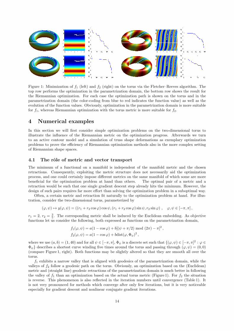
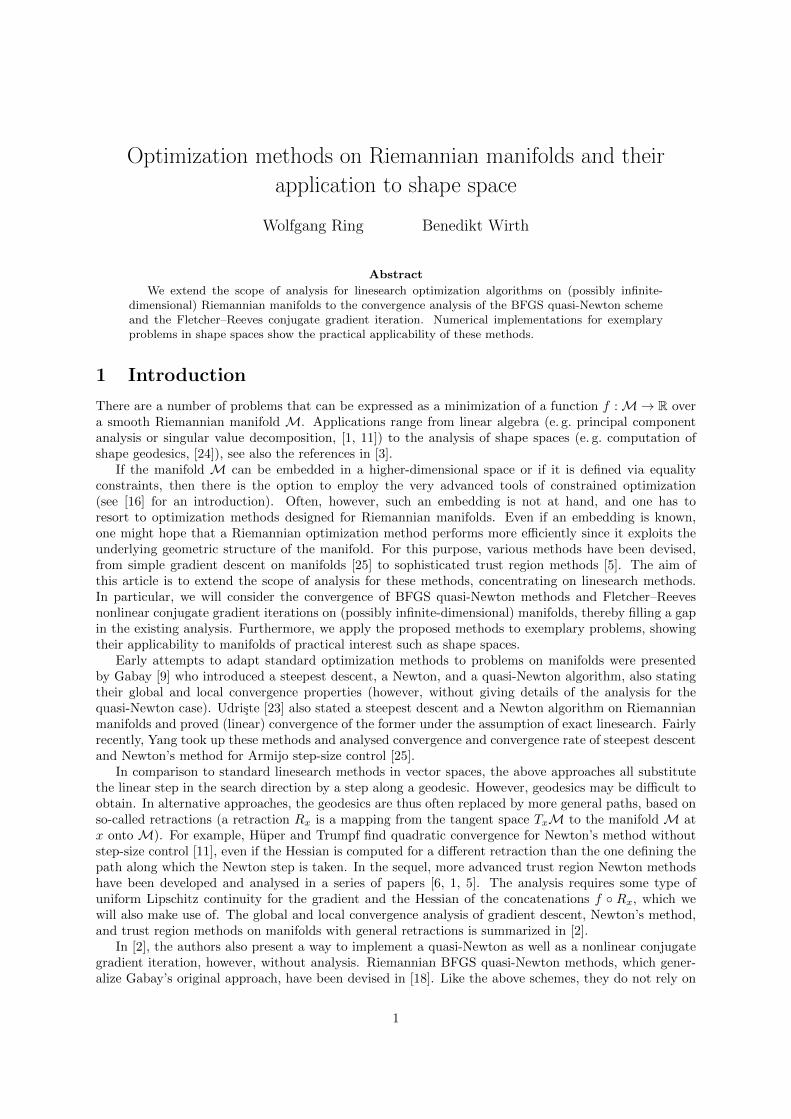
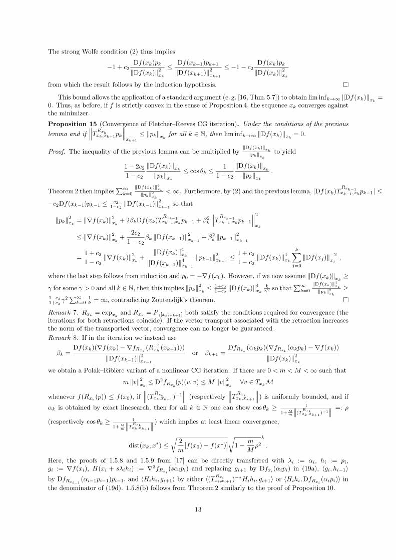
Figure 1: Minimization of f1 (left) and f2 (right) on the torus via the Fletcher–Reeves algorithm. Thetop row performs the optimization in the parametrization domain, the bottom row shows the result forthe Riemannian optimization. For each case the optimization path is shown on the torus and in theparametrization domain (the color-coding from blue to red indicates the function value) as well as theevolution of the function values. Obviously, optimization in the parametrization domain is more suitablefor f1, whereas Riemannian optimization with the torus metric is more suitable for f2.

4 Numerical examples

In this section we will first consider simple optimization problems on the two-dimensional torus toillustrate the influence of the Riemannian metric on the optimization progress. Afterwards we turnto an active contour model and a simulation of truss shape deformations as exemplary optimizationproblems to prove the efficiency of Riemannian optimization methods also in the more complex settingof Riemannian shape spaces.

4.1 The role of metric and vector transport

The minimum of a functional on a manifold is independent of the manifold metric and the chosenretractions. Consequently, exploiting the metric structure does not necessarily aid the optimizationprocess, and one could certainly impose different metrics on the same manifold of which some are morebeneficial for the optimization problem at hand than others. The optimal pair of a metric and aretraction would be such that one single gradient descent step already hits the minimum. However, thedesign of such pairs requires far more effort than solving the optimization problem in a suboptimal way.

Often, a certain metric and retraction fit naturally to the optimization problem at hand. For illus-tration, consider the two-dimensional torus, parameterized by

(ϕ,ψ) 7→ y(ϕ,ψ) = ((r1 + r2 cosϕ) cosψ, (r1 + r2 cosϕ) sinψ, r2 sinϕ) , ϕ, ψ ∈ [−π, π] ,

r1 = 2, r2 = 35 . The corresponding metric shall be induced by the Euclidean embedding. As objective

functions let us consider the following, both expressed as functions on the parametrization domain,

f1(ϕ,ψ) = a(1− cosϕ) + b[(ψ + π/2) mod (2π)− π]2 ,

f2(ϕ,ψ) = a(1− cosϕ) + bdist(ϕ,Φψ)2 ,

where we use (a, b) = (1, 40) and for all ψ ∈ [−π, π], Φψ is a discrete set such that {(ϕ,ψ) ∈ [−π, π]2 : ϕ ∈Φψ} describes a shortest curve winding five times around the torus and passing through (ϕ,ψ) = (0, 0)(compare Figure 1, right). Both functions may be slightly altered so that they are smooth all over thetorus.

f1 exhibits a narrow valley that is aligned with geodesics of the parametrization domain, while thevalleys of f2 follow a geodesic path on the torus. Obviously, an optimization based on the (Euclidean)metric and (straight line) geodesic retractions of the parametrization domain is much better in followingthe valley of f1 than an optimization based on the actual torus metric (Figure 1). For f2 the situationis reverse. This phenomenon is also reflected in the iteration numbers until convergence (Table 1). Itis not very pronounced for methods which converge after only few iterations, but it is very noticeableespecially for gradient descent and nonlinear conjugate gradient iterations.

14

objective f1 objective f2parametr. metric torus metric parametr. metric torus metric

gradient descent 213 890 9537 2212Newton descent 22 28 38 29BFGS quasi-Newton 16 28 55 69Fletcher–Reeves NCG 34 120 98 29

Table 1: Iteration numbers for minimization of f1 and f2 with different methods. The iteration is stoppedas soon as ‖(∂fi∂ϕ ,

∂fi∂ψ )‖`2 < 10−3. As retractions we use the exponential maps with respect to the metric

of the parametrization domain and of the torus, respectively. The BFGS and NCG method employ thecorresponding parallel transport.

0 50 100 150

10−6

10−4

10−2

100

iteration number

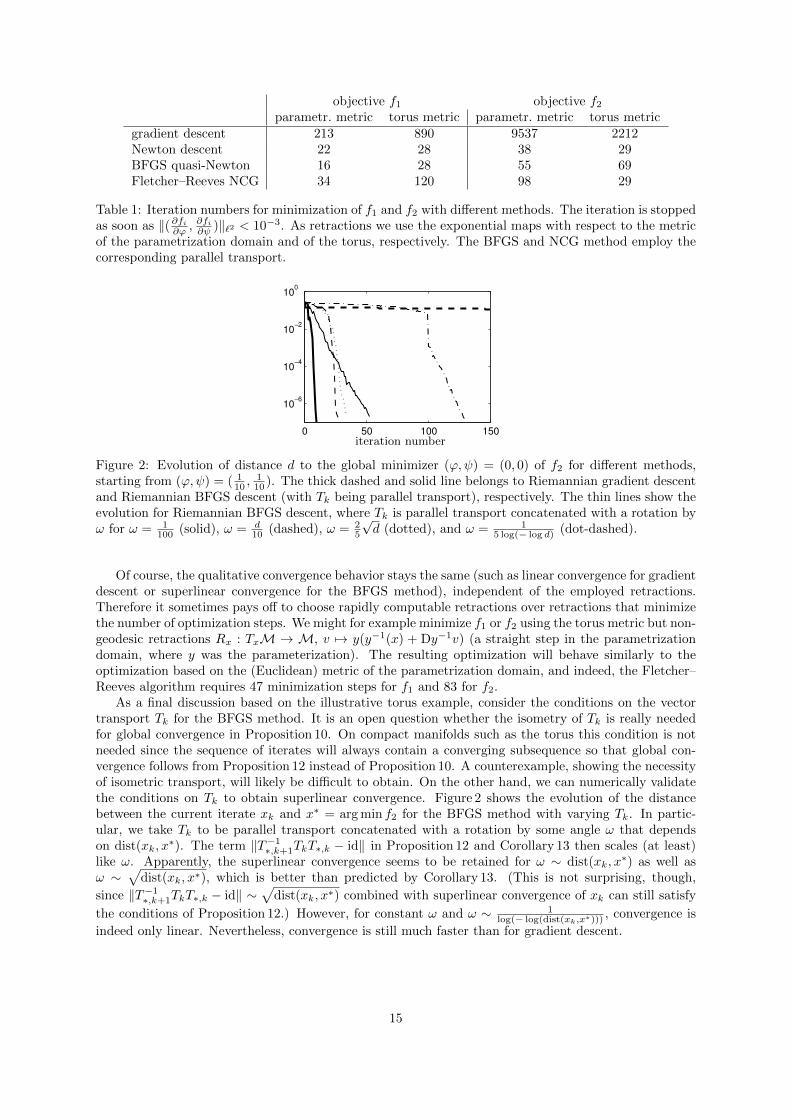
Figure 2: Evolution of distance d to the global minimizer (ϕ,ψ) = (0, 0) of f2 for different methods,starting from (ϕ,ψ) = ( 1

10 ,110 ). The thick dashed and solid line belongs to Riemannian gradient descent

and Riemannian BFGS descent (with Tk being parallel transport), respectively. The thin lines show theevolution for Riemannian BFGS descent, where Tk is parallel transport concatenated with a rotation byω for ω = 1

100 (solid), ω = d10 (dashed), ω = 2

5

√d (dotted), and ω = 1

5 log(− log d) (dot-dashed).

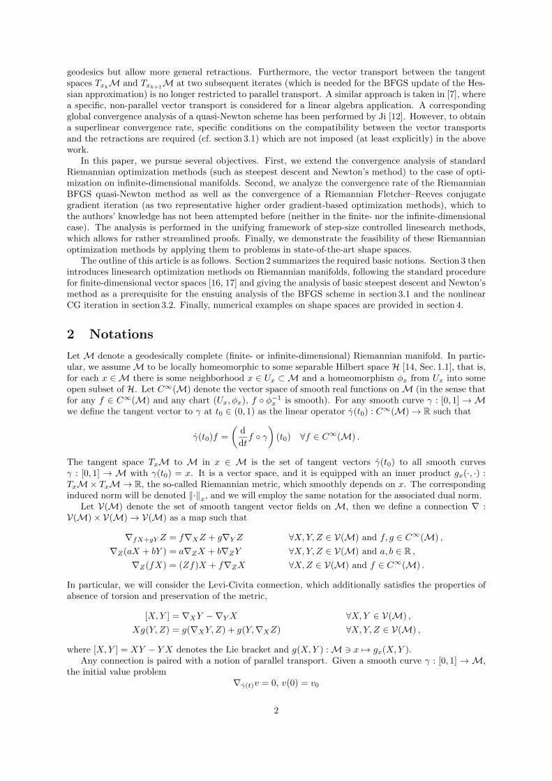
Of course, the qualitative convergence behavior stays the same (such as linear convergence for gradientdescent or superlinear convergence for the BFGS method), independent of the employed retractions.Therefore it sometimes pays off to choose rapidly computable retractions over retractions that minimizethe number of optimization steps. We might for example minimize f1 or f2 using the torus metric but non-geodesic retractions Rx : TxM → M, v 7→ y(y−1(x) + Dy−1v) (a straight step in the parametrizationdomain, where y was the parameterization). The resulting optimization will behave similarly to theoptimization based on the (Euclidean) metric of the parametrization domain, and indeed, the Fletcher–Reeves algorithm requires 47 minimization steps for f1 and 83 for f2.

As a final discussion based on the illustrative torus example, consider the conditions on the vectortransport Tk for the BFGS method. It is an open question whether the isometry of Tk is really neededfor global convergence in Proposition 10. On compact manifolds such as the torus this condition is notneeded since the sequence of iterates will always contain a converging subsequence so that global con-vergence follows from Proposition 12 instead of Proposition 10. A counterexample, showing the necessityof isometric transport, will likely be difficult to obtain. On the other hand, we can numerically validatethe conditions on Tk to obtain superlinear convergence. Figure 2 shows the evolution of the distancebetween the current iterate xk and x∗ = arg min f2 for the BFGS method with varying Tk. In partic-ular, we take Tk to be parallel transport concatenated with a rotation by some angle ω that dependson dist(xk, x

∗). The term ‖T−1∗,k+1TkT∗,k − id‖ in Proposition 12 and Corollary 13 then scales (at least)like ω. Apparently, the superlinear convergence seems to be retained for ω ∼ dist(xk, x

∗) as well asω ∼

√dist(xk, x∗), which is better than predicted by Corollary 13. (This is not surprising, though,

since ‖T−1∗,k+1TkT∗,k − id‖ ∼√

dist(xk, x∗) combined with superlinear convergence of xk can still satisfy

the conditions of Proposition 12.) However, for constant ω and ω ∼ 1log(− log(dist(xk,x∗)))

, convergence is

indeed only linear. Nevertheless, convergence is still much faster than for gradient descent.

15

4.2 Riemannian optimization in the space of smooth closed curves

Riemannian optimization on the Stiefel manifold has been applied successfully and efficiently to severallinear algebra problems, from low rank approximation [7] to eigenvalue computation [18]. The sameconcepts can be transferred to efficient optimization methods in the space of closed smooth curves, usingthe shape space and description of curves introduced by Younes et al. [26]. They represent a curvec : [0, 1]→ C ≡ R2 by two functions e, g : [0, 1]→ R via

c(θ) = c(0) +1

2

∫ θ

0

(e+ ig)2 dϑ .

The conditions that the curve be closed, c(1) = c(0), and of unit length, 1 =∫ 1

0|c′(θ)|dθ, result in the

fact that e and g are orthonormal in L2([0, 1]), thus (e, g) forms an element of the Stiefel manifold

St(2, L2([0, 1])) ={

(e, g) ∈ L2([0, 1]) : ‖e‖L2([0,1]) = ‖g‖L2([0,1]) = 1, (e, g)L2([0,1]) = 0}.

The Riemannian metric of the Stiefel manifold can now be imposed on the the space of smooth closedcurves with unit length and fixed base point, which was shown to be equivalent to endowing this shapespace with a Sobolev-type metric [26].

For general closed curves we follow Sundaramoorthi et al. [22] and represent a curve c by an element(c0, ρ, (e, g)) of R2 × R× St(2, L2([0, 1])) via

c(θ) = c0 +exp ρ

2

∫ θ

0

(e+ ig)2 dϑ .

c0 describes the curve base point and exp ρ its length. (Note that Sundaramoorthi et al. choose c0 asthe curve centroid. Choosing the base point instead simplifies the notation a little and yields the samequalitative behavior.) Sundaramoorthi et al. have shown the corresponding Riemannian metric to beequivalent to the very natural metric

g[c](h, k) = ht · kt + λlhlkl + λd

∫[c]

dhd

ds· dkd

dsds

on the tangent space of curve variations h, k : [c] → R2, where [c] is the image of c : [0, 1] → R2, sdenotes arclength, and λl, λd > 0. Here, ht and hl are the Gateaux derivatives of the curve centroid (inour case the base point) and the logarithm of the curve length for curve variation in direction h, andhd = ht + hl(c− c0) (analogous for k). By [10] this yields a geodesically complete shape space in whichthere is a closed formula for the exponential map [22], lending itself for Riemannian optimization. (Notethat simple L2-type metrics in the space of curves can in general not be used since the resulting spacesusually are degenerate [15]: They exhibit paths of arbitrarily small length between any two curves.)

To illustrate the efficiency of Riemannian optimization in this context we consider the task of imagesegmentation via active contours without edges as proposed by Chan and Vese [8]. For a given gray scaleimage u : [0, 1]2 → R we would like to minimize the objective functional

f([c]) = a1

(∫int[c]

(ui − u)2 dx+

∫ext[c]

(ue − u)2 dx

)+ a2

∫[c]

ds ,

where a1, a2 > 0, ui and ue are given gray values, and int[c] and ext[c] denote the interior and exteriorof [c]. The first two terms indicate that [c] should enclose the image region where u is close to ui and farfrom ue, while the third term acts as a regularizer and measures the curve length.

We interpret the curve c as an element of the above Riemannian manifold R2 × R× St(2, L2([0, 1]))and add an additional term to the objective functional that prefers a uniform curve parametrization.The objective functional then reads

f(c0, ρ, (e, g)) = a1

(∫int[(c0,ρ,(e,g))]

(ui − u)2 dx+

∫ext[(c0,ρ,(e,g))]

(ue − u)2 dx

)+a2 exp(ρ)+a3

∫ 1

0

(e2+g2)2 dϑ ,

16

0 20 4010

−8

10−4

100

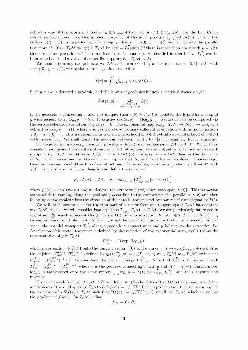
Figure 3: Curve evolution during BFGS minimization of f . The curve is depicted at steps 0, 1, 2, 3, 4,7, and after convergence. Additionally we show the evolution of the function value f(ck)−minc f(c).

non-geodesic retr. geodesic retr.gradient flow 4207 4207gradient descent 1076 1064BFGS quasi-Newton 44 45Fletcher–Reeves NCG 134 220

Table 2: Iteration numbers for minimization of f with different methods. The iteration is stopped assoon as the derivative of the discretized functional f has `2-norm less than 10−3. For the gradient flowdiscretization we employ a stepsize of 0.001, which is roughly the largest stepsize for which the curvestays within the image domain during the whole iteration.

where we choose (a1, a2, a3) = (50, 1, 1). For numerical implementation, e and g are discretized aspiecewise constant functions on an equispaced grid over [0, 1], and the image u is given as pixel valueson a uniform quadrilateral grid, where we interpolate bilinearly between the nodes.

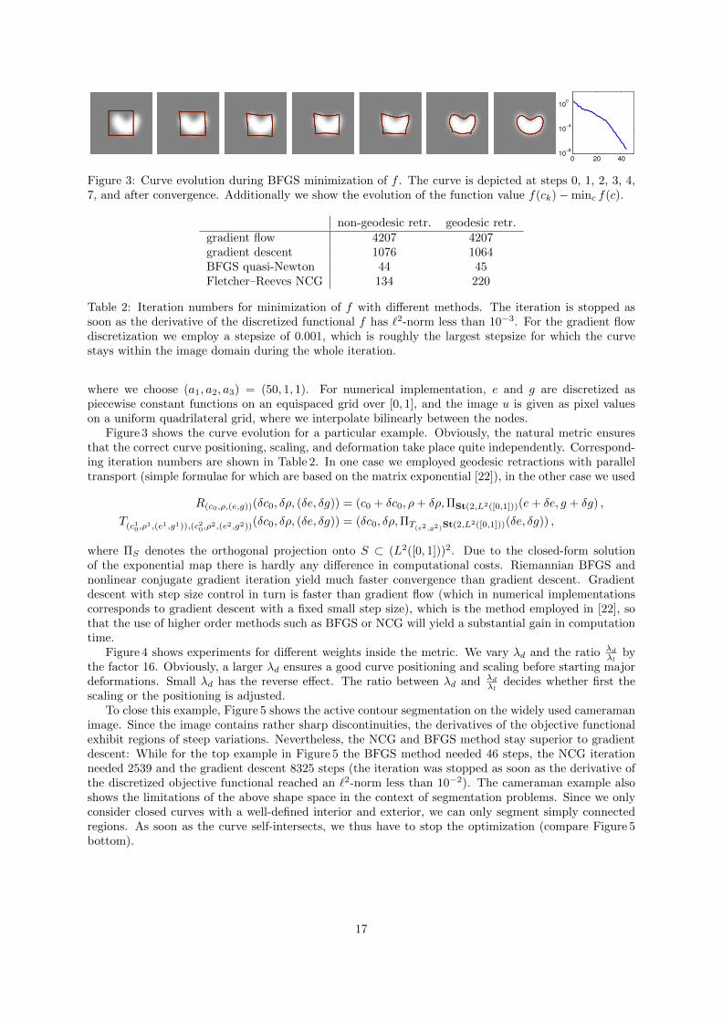
Figure 3 shows the curve evolution for a particular example. Obviously, the natural metric ensuresthat the correct curve positioning, scaling, and deformation take place quite independently. Correspond-ing iteration numbers are shown in Table 2. In one case we employed geodesic retractions with paralleltransport (simple formulae for which are based on the matrix exponential [22]), in the other case we used

R(c0,ρ,(e,g))(δc0, δρ, (δe, δg)) = (c0 + δc0, ρ+ δρ,ΠSt(2,L2([0,1]))(e+ δe, g + δg) ,

T(c10,ρ1,(e1,g1)),(c20,ρ2,(e2,g2))(δc0, δρ, (δe, δg)) = (δc0, δρ,ΠT(e2,g2)St(2,L

2([0,1]))(δe, δg)) ,

where ΠS denotes the orthogonal projection onto S ⊂ (L2([0, 1]))2. Due to the closed-form solutionof the exponential map there is hardly any difference in computational costs. Riemannian BFGS andnonlinear conjugate gradient iteration yield much faster convergence than gradient descent. Gradientdescent with step size control in turn is faster than gradient flow (which in numerical implementationscorresponds to gradient descent with a fixed small step size), which is the method employed in [22], sothat the use of higher order methods such as BFGS or NCG will yield a substantial gain in computationtime.

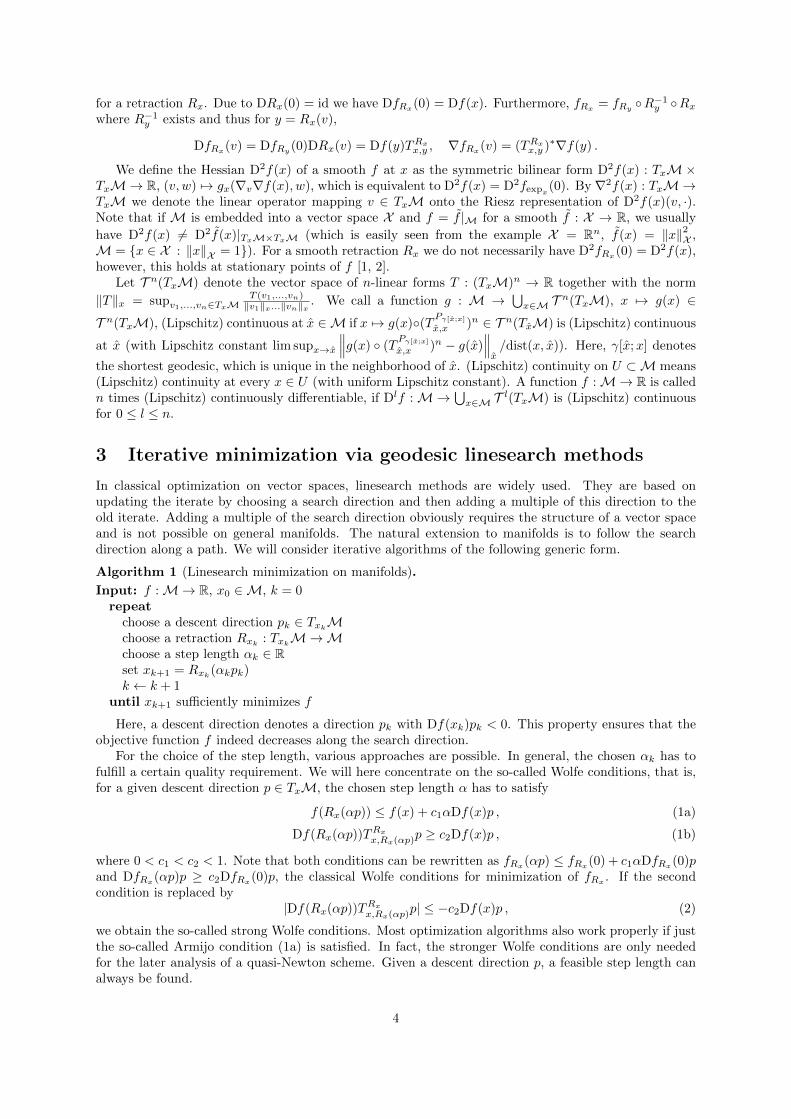
Figure 4 shows experiments for different weights inside the metric. We vary λd and the ratio λdλl

bythe factor 16. Obviously, a larger λd ensures a good curve positioning and scaling before starting majordeformations. Small λd has the reverse effect. The ratio between λd and λd

λldecides whether first the

scaling or the positioning is adjusted.To close this example, Figure 5 shows the active contour segmentation on the widely used cameraman

image. Since the image contains rather sharp discontinuities, the derivatives of the objective functionalexhibit regions of steep variations. Nevertheless, the NCG and BFGS method stay superior to gradientdescent: While for the top example in Figure 5 the BFGS method needed 46 steps, the NCG iterationneeded 2539 and the gradient descent 8325 steps (the iteration was stopped as soon as the derivative ofthe discretized objective functional reached an `2-norm less than 10−2). The cameraman example alsoshows the limitations of the above shape space in the context of segmentation problems. Since we onlyconsider closed curves with a well-defined interior and exterior, we can only segment simply connectedregions. As soon as the curve self-intersects, we thus have to stop the optimization (compare Figure 5bottom).

17

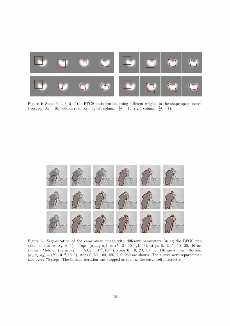
Figure 4: Steps 0, 1, 3, 5 of the BFGS optimization, using different weights in the shape space metric(top row: λd = 16; bottom row: λd = 1; left column: λd

λl= 16; right column: λd

λl= 1).

Figure 5: Segmentation of the cameraman image with different parameters (using the BFGS iter-ation and λl = λd = 1). Top: (a1, a2, a3) = (50, 3 · 10−1, 10−3), steps 0, 1, 5, 10, 20, 46 areshown. Middle: (a1, a2, a3) = (50, 8 · 10−2, 10−3), steps 0, 10, 20, 40, 60, 116 are shown. Bottom:(a1, a2, a3) = (50, 10−2, 10−3), steps 0, 50, 100, 150, 200, 250 are shown. The curves were reparameter-ized every 70 steps. The bottom iteration was stopped as soon as the curve self-intersected.

18

4.3 Riemannian optimization in the space of truss shapes

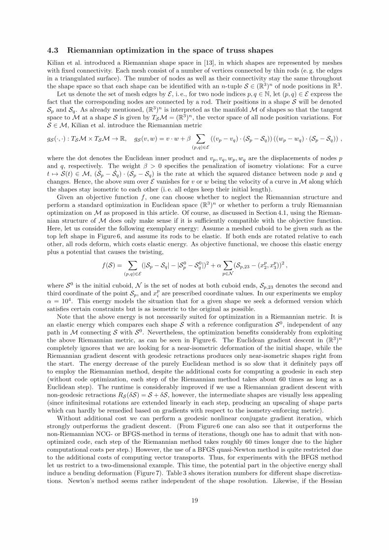
Kilian et al. introduced a Riemannian shape space in [13], in which shapes are represented by mesheswith fixed connectivity. Each mesh consist of a number of vertices connected by thin rods (e. g. the edgesin a triangulated surface). The number of nodes as well as their connectivity stay the same throughoutthe shape space so that each shape can be identified with an n-tuple S ∈ (R3)n of node positions in R3.

Let us denote the set of mesh edges by E , i. e., for two node indices p, q ∈ N, let (p, q) ∈ E express thefact that the corresponding nodes are connected by a rod. Their positions in a shape S will be denotedSp and Sq. As already mentioned, (R3)n is interpreted as the manifoldM of shapes so that the tangentspace toM at a shape S is given by TSM = (R3)n, the vector space of all node position variations. ForS ∈ M, Kilian et al. introduce the Riemannian metric

gS(·, ·) : TSM× TSM→ R, gS(v, w) = v · w + β∑

(p,q)∈E

((vp − vq) · (Sp − Sq)) ((wp − wq) · (Sp − Sq)) ,

where the dot denotes the Euclidean inner product and vp, vq, wp, wq are the displacements of nodes pand q, respectively. The weight β > 0 specifies the penalization of isometry violations: For a curvet 7→ S(t) ∈ M, (Sp − Sq) · (Sp − Sq) is the rate at which the squared distance between node p and qchanges. Hence, the above sum over E vanishes for v or w being the velocity of a curve inM along whichthe shapes stay isometric to each other (i. e. all edges keep their initial length).

Given an objective function f , one can choose whether to neglect the Riemannian structure andperform a standard optimization in Euclidean space (R3)n or whether to perform a truly Riemannianoptimization onM as proposed in this article. Of course, as discussed in Section 4.1, using the Rieman-nian structure of M does only make sense if it is sufficiently compatible with the objective function.Here, let us consider the following exemplary energy: Assume a meshed cuboid to be given such as thetop left shape in Figure 6, and assume its rods to be elastic. If both ends are rotated relative to eachother, all rods deform, which costs elastic energy. As objective functional, we choose this elastic energyplus a potential that causes the twisting,

f(S) =∑

(p,q)∈E

(|Sp − Sq| − |S0p − S0q |)2 + α∑p∈N

(Sp,23 − (xp2, xp3))2 ,

where S0 is the initial cuboid, N is the set of nodes at both cuboid ends, Sp,23 denotes the second andthird coordinate of the point Sp, and xpi are prescribed coordinate values. In our experiments we employα = 104. This energy models the situation that for a given shape we seek a deformed version whichsatisfies certain constraints but is as isometric to the original as possible.

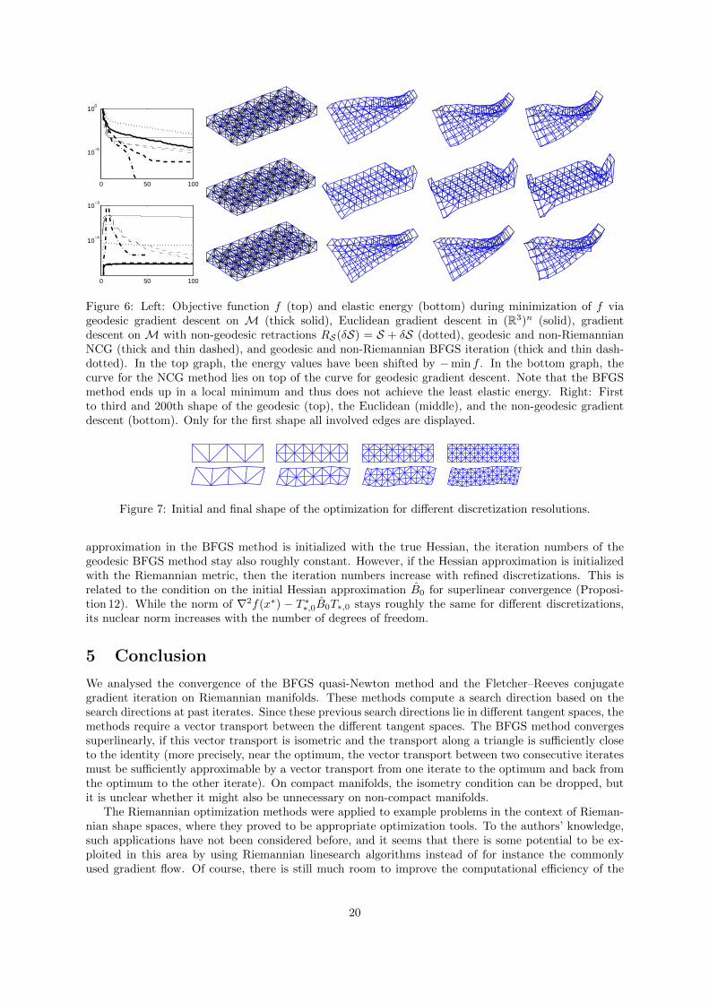
Note that the above energy is not necessarily suited for optimization in a Riemannian metric. It isan elastic energy which compares each shape S with a reference configuration S0, independent of anypath in M connecting S with S0. Nevertheless, the optimization benefits considerably from exploitingthe above Riemannian metric, as can be seen in Figure 6. The Euclidean gradient descent in (R3)n

completely ignores that we are looking for a near-isometric deformation of the initial shape, while theRiemannian gradient descent with geodesic retractions produces only near-isometric shapes right fromthe start. The energy decrease of the purely Euclidean method is so slow that it definitely pays offto employ the Riemannian method, despite the additional costs for computing a geodesic in each step(without code optimization, each step of the Riemannian method takes about 60 times as long as aEuclidean step). The runtime is considerably improved if we use a Riemannian gradient descent withnon-geodesic retractions RS(δS) = S + δS, however, the intermediate shapes are visually less appealing(since infinitesimal rotations are extended linearly in each step, producing an upscaling of shape partswhich can hardly be remedied based on gradients with respect to the isometry-enforcing metric).

Without additional cost we can perform a geodesic nonlinear conjugate gradient iteration, whichstrongly outperforms the gradient descent. (From Figure 6 one can also see that it outperforms thenon-Riemannian NCG- or BFGS-method in terms of iterations, though one has to admit that with non-optimized code, each step of the Riemannian method takes roughly 60 times longer due to the highercomputational costs per step.) However, the use of a BFGS quasi-Newton method is quite restricted dueto the additional costs of computing vector transports. Thus, for experiments with the BFGS methodlet us restrict to a two-dimensional example. This time, the potential part in the objective energy shallinduce a bending deformation (Figure 7). Table 3 shows iteration numbers for different shape discretiza-tions. Newton’s method seems rather independent of the shape resolution. Likewise, if the Hessian

19

0 50 100

10−5

100

0 50 100

10−4

10−3

Figure 6: Left: Objective function f (top) and elastic energy (bottom) during minimization of f viageodesic gradient descent on M (thick solid), Euclidean gradient descent in (R3)n (solid), gradientdescent on M with non-geodesic retractions RS(δS) = S + δS (dotted), geodesic and non-RiemannianNCG (thick and thin dashed), and geodesic and non-Riemannian BFGS iteration (thick and thin dash-dotted). In the top graph, the energy values have been shifted by −min f . In the bottom graph, thecurve for the NCG method lies on top of the curve for geodesic gradient descent. Note that the BFGSmethod ends up in a local minimum and thus does not achieve the least elastic energy. Right: Firstto third and 200th shape of the geodesic (top), the Euclidean (middle), and the non-geodesic gradientdescent (bottom). Only for the first shape all involved edges are displayed.

Figure 7: Initial and final shape of the optimization for different discretization resolutions.

approximation in the BFGS method is initialized with the true Hessian, the iteration numbers of thegeodesic BFGS method stay also roughly constant. However, if the Hessian approximation is initializedwith the Riemannian metric, then the iteration numbers increase with refined discretizations. This isrelated to the condition on the initial Hessian approximation B0 for superlinear convergence (Proposi-tion 12). While the norm of ∇2f(x∗) − T ∗∗,0B0T∗,0 stays roughly the same for different discretizations,its nuclear norm increases with the number of degrees of freedom.

5 Conclusion

We analysed the convergence of the BFGS quasi-Newton method and the Fletcher–Reeves conjugategradient iteration on Riemannian manifolds. These methods compute a search direction based on thesearch directions at past iterates. Since these previous search directions lie in different tangent spaces, themethods require a vector transport between the different tangent spaces. The BFGS method convergessuperlinearly, if this vector transport is isometric and the transport along a triangle is sufficiently closeto the identity (more precisely, near the optimum, the vector transport between two consecutive iteratesmust be sufficiently approximable by a vector transport from one iterate to the optimum and back fromthe optimum to the other iterate). On compact manifolds, the isometry condition can be dropped, butit is unclear whether it might also be unnecessary on non-compact manifolds.

The Riemannian optimization methods were applied to example problems in the context of Rieman-nian shape spaces, where they proved to be appropriate optimization tools. To the authors’ knowledge,such applications have not been considered before, and it seems that there is some potential to be ex-ploited in this area by using Riemannian linesearch algorithms instead of for instance the commonlyused gradient flow. Of course, there is still much room to improve the computational efficiency of the

20

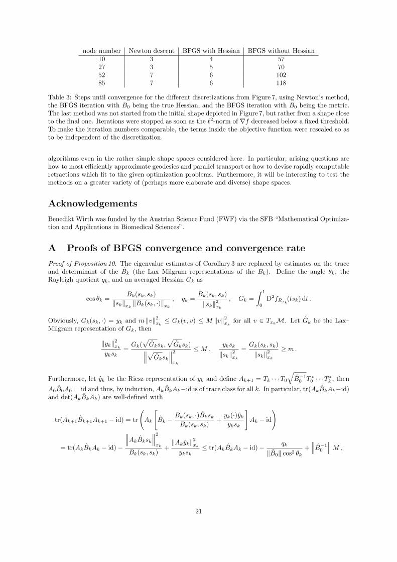
node number Newton descent BFGS with Hessian BFGS without Hessian10 3 4 5727 3 5 7052 7 6 10285 7 6 118

Table 3: Steps until convergence for the different discretizations from Figure 7, using Newton’s method,the BFGS iteration with B0 being the true Hessian, and the BFGS iteration with B0 being the metric.The last method was not started from the initial shape depicted in Figure 7, but rather from a shape closeto the final one. Iterations were stopped as soon as the `2-norm of ∇f decreased below a fixed threshold.To make the iteration numbers comparable, the terms inside the objective function were rescaled so asto be independent of the discretization.

algorithms even in the rather simple shape spaces considered here. In particular, arising questions arehow to most efficiently approximate geodesics and parallel transport or how to devise rapidly computableretractions which fit to the given optimization problems. Furthermore, it will be interesting to test themethods on a greater variety of (perhaps more elaborate and diverse) shape spaces.

Acknowledgements

Benedikt Wirth was funded by the Austrian Science Fund (FWF) via the SFB “Mathematical Optimiza-tion and Applications in Biomedical Sciences”.

A Proofs of BFGS convergence and convergence rate

Proof of Proposition 10. The eigenvalue estimates of Corollary 3 are replaced by estimates on the traceand determinant of the Bk (the Lax–Milgram representations of the Bk). Define the angle θk, theRayleigh quotient qk, and an averaged Hessian Gk as

cos θk =Bk(sk, sk)

‖sk‖xk ‖Bk(sk, ·)‖xk, qk =

Bk(sk, sk)

‖sk‖2xk, Gk =

∫ 1

0

D2fRxk(tsk) dt .

Obviously, Gk(sk, ·) = yk and m ‖v‖2xk ≤ Gk(v, v) ≤ M ‖v‖2xk for all v ∈ TxkM. Let Gk be the Lax–Milgram representation of Gk, then

‖yk‖2xkyksk

=Gk(

√Gksk,

√Gksk)∥∥∥√Gksk∥∥∥2xk

≤M ,yksk

‖sk‖2xk=Gk(sk, sk)

‖sk‖2xk≥ m.

Furthermore, let yk be the Riesz representation of yk and define Ak+1 = Tk · · ·T0√B−10 T ∗0 · · ·T ∗k , then

A0B0A0 = id and thus, by induction, AkBkAk−id is of trace class for all k. In particular, tr(AkBkAk−id)and det(AkBkAk) are well-defined with

tr(Ak+1Bk+1Ak+1 − id) = tr

(Ak

[Bk −

Bk(sk, ·)BkskBk(sk, sk)

+yk(·)ykyksk

]Ak − id

)

= tr(AkBkAk − id)−

∥∥∥AkBksk∥∥∥2xk

Bk(sk, sk)+‖Akyk‖2xkyksk

≤ tr(AkBkAk − id)− qk

‖B0‖ cos2 θk+∥∥∥B−10

∥∥∥M ,

21

det(Ak+1Bk+1Ak+1) = det

(Ak

[Bk −

Bk(sk, ·)BkskBk(sk, sk)

+yk(·)ykyksk

]Ak

)

= det

(Ak

√Bk[I − s⊗ s + y⊗ y]

√BkAk

)= det(AkBkAk) det(I − s⊗ s + y⊗ y)

= det(AkBkAk)(1+λ1)(1+λ2) = det(AkBkAk)yksk

Bk(sk, sk)= det(AkBkAk)

yksk

qk ‖sk‖2xk≥ m

qkdet(AkBkAk) .

where we have used the abbreviations s =√Bksk/

√Bk(sk, sk), y = B

− 12

k yk√yksk, λ1,2 = gxk(s, s) +

gxk(y, y)±√

(gxk(s, s) + gxk(y, y))2 − gxk(s, y)2 (the two nonzero eigenvalues of−s⊗s+y⊗y) as well as thefact that isometries leave the determinant and trace unchanged, the definition det(I+B) = Πi(1+λi(B))for trace class operators B [20, Chp. 3] (where λi(B) are the corresponding eigenvalues), and the productrule for determinants [20, Thm. 3.5]. Next, define Ψ(B) = tr(B − id)− log det B, which is non-negativefor positive definite B by Lidskii’s theorem [20, Thm. 3.7]. By induction,

0 ≤ Ψ(Ak+1Bk+1Ak+1) ≤ Ψ(A0B0A0)

+

k∑i=0

((∥∥∥B−10

∥∥∥M − logm− 1) + log(‖B0‖ cos2 θi) +

[1− qi

‖B0‖ cos2 θi+ log

qi

‖B0‖ cos2 θi

]).

We now show that for any 0 < r < 1 there are constants κ, ρ, σ > 0 such that for any k ∈ N there are atleast br(k + 1)c indices i in {0, . . . , k} with cos θi ≥ κ and ρ ≤ qi

cos θi≤ σ. Let us abbreviate

ηi = − log(‖B0‖ cos2 θi)− li = − log(‖B0‖ cos2 θi)−

[1− qi

‖B0‖ cos2 θi+ log

qi

‖B0‖ cos2 θi

]and denote the br(k + 1)cth smallest among η0, . . . , ηk by ηk. Now let I = {i ∈ {0, . . . , k} : ηi > ηk}.For all br(k + 1)c indices i ∈ {0, . . . , k} \ I we have

ηi ≤ ηk ≤1

|I|∑j∈I

ηj ≤1

1− r1

k + 1

k∑j=0

ηj ≤1

1− r

(Ψ(id)

k + 1+ (∥∥∥B−10

∥∥∥M − logm− 1)

)≤ c

for some constant c, where the second last inequality comes from the estimate for Ψ(Ak+1Bk+1Ak+1)above. Hence, log(‖B0‖ cos2 θi) and li must be bounded from below for these indices i, from which we

first obtain

√‖B0‖ ≥

√‖B0‖ cos θi ≥ exp −c2 =:

√‖B0‖κ and then also boundedness of qi

cos θiabove and

below by some σ and ρ (due to the concavity and continuity of g(x) = 1−x+ log x with g(x)→ −∞ forx→ 0 and x→∞). Furthermore, for the same indices i, (1b) implies −c2Df(xi)pi ≥ −DfRxi (αipi)pi =

−Df(xi)pi − αi∫ 1

0D2fRxi (tαipi)(pi, pi) dt ≥ −Df(xi)pi − αiM ‖pi‖2xi so that

αi ≥ −Df(xi)pi

‖pi‖2xi

1− c2M

=1− c2M

qi ≥1− c2M

κρ .

Equation (1a) then implies

f(xi)− f(xi+1) ≥ −αic1Df(xi)pi ≥1− c2M

κρc1cos2 θiqi

‖Df(xi)‖2xi ≥1− c2M

κρc1κ

σ2m(f(xi)− f(x∗)) ,

where in the last step we used f(x) − f(x∗) ≤ 12m ‖Df(x)‖2x, which follows from separately minimizing

for x ∈M the right-hand and the left-hand side of the inequality

f(x)− f(x) = Df(x)R−1x (x) +1

2D2fRx(tR−1x (x))(R−1x (x), R−1x (x)) ≥ Df(x)R−1x (x) +

m

2

∥∥R−1x (x)∥∥2x

with some t ∈ [0, 1]. Due to the monotonicity of the f(xk) and the above estimates for the br(k + 1)cindices i with ηi ≤ ηk, we arrive at

f(xk)− f(x∗) ≤(

1− 1− c2M

c1κ2ρ

σ2m

)br(k+1)c

(f(x0)− f(x∗)) ∀k ∈ N .

22

(From the non-negativity of f(xk)− f(x∗) and f(x0)− f(x∗) we additionally see that the bounds σ andρ satisfy σ

ρ ≥1−c2M c1κ

22m.)

Proof of Proposition 12. Let us define G = ∇2f(x∗) as well as

sk = G12T−1∗,ksk , yk = G−

12T ∗∗,kyk , Bk = G−

12T ∗∗,kBkT∗,kG

− 12 , TG,k = G

12T−1∗,kT

−1k T∗,k+1G

− 12 ,

where (as before) yk and Bk are the Riesz and Lax–Milgram representation of yk and Bk. Note

Bk+1 = T ∗G,k

[Bk −

gx∗(Bksk, ·)Bkskgx∗(Bksk, sk)

+gx∗(yk, ·)ykgx∗(yk, sk)

]TG,k

as well as tr(T ∗G,kBTG,k) = trB + tr((T ∗G,k − id)B) + tr(B(TG,k − id)) + tr((T ∗G,k − id)B(TG,k − id)) forany trace class operator B : Tx∗M→ Tx∗M so that

tr(T ∗G,kBTG,k) ≤ trB + ‖B‖1(

2∥∥∥G 1

2

∥∥∥ ∥∥∥G− 12

∥∥∥ δk + ‖G‖∥∥G−1∥∥ δ2k) ≤ trB + C ‖B‖1 δk (8)

with δk =∥∥∥T−1∗,kT−1k T∗,k+1 − id

∥∥∥, where C is chosen large enough so that the above holds for all k. In

the above we have used that trace and nuclear norm can be expressed as trB =∑i gx∗(ei, Bei) and

‖B‖1 =∑i |gx∗(ei, Bei)| for any orthonormal basis (ei)i of Tx∗M so that trB ≤ ‖B‖1 and ‖AB‖1 =∑

i |gx∗(ei, ABei)| ≤ ‖A‖∑i |gx∗(ei, Bei)| = ‖A‖ ‖B‖1 for any bounded operator A : Tx∗M → Tx∗M.

Furthermore, let Gk be the Lax–Milgram representation of Gk from the proof of Proposition 10, then

‖yk − sk‖x∗ =∥∥∥G− 1

2 (T ∗∗,kGkT∗,k −G)G−12 sk

∥∥∥x∗≤ cεk ‖sk‖x∗

with c =∥∥G−1∥∥ and εk =

∥∥∥T ∗∗,kGkT∗,k −G∥∥∥. We deduce

mk :=gx∗(yk, sk)

‖sk‖2x∗≥ 1− cεk , Mk :=

‖yk‖2x∗gx∗(yk, sk)

≤ 1 + cεk

for k large enough, which follows from ‖yk‖2x∗−2gx∗(yk, sk)+‖sk‖2x∗ = ‖yk − sk‖2x∗ ≤ c2ε2k ‖sk‖2x∗ as well

as |‖yk‖x∗ − ‖sk‖x∗ | ≤ ‖yk − sk‖x∗ ≤ cεk ‖sk‖x∗ so that (1− cεk) ‖sk‖x∗ ≤ ‖yk‖x∗ ≤ (1 + cεk) ‖sk‖x∗ .Next, let us introduce

qk =gx∗(sk, Bksk)

‖sk‖2x∗, cos θk =

gx∗(sk, Bksk)

‖sk‖x∗∥∥∥Bksk∥∥∥

x∗

.

Using∥∥∥T ∗G,kBTG,k∥∥∥

1=∥∥∥B+(T ∗G,k−id)B+B(TG,k−id)+(T ∗G,k−id)B(TG,k−id)

∥∥∥1≤‖B‖1+

∥∥∥(T ∗G,k−id)B∥∥∥1+

‖B(TG,k − id)‖1 +∥∥∥(T ∗G,k − id)B(TG,k − id)

∥∥∥1≤ ‖B‖1 + ‖B‖1

(2∥∥∥G 1

2

∥∥∥ ∥∥∥G− 12

∥∥∥ δk + ‖G‖∥∥G−1∥∥ δ2k) ≤

‖B‖1 + C ‖B‖1 δk for any trace class operator B, the nuclear norm of Bk+1 − id can be bounded asfollows,∥∥∥Bk+1 − id

∥∥∥1

=

∥∥∥∥∥T ∗G,k[Bk − id− gx∗(Bksk, ·)Bksk

gx∗(Bksk, sk)+gx∗(yk, ·)ykgx∗(yk, sk)

]TG,k + T ∗G,kTG,k − id

∥∥∥∥∥1

≤∥∥T ∗G,kTG,k − id

∥∥1

+ (1 + Cδk)

(∥∥∥Bk − id∥∥∥1

+qk

cos2 θk+ Mk

)≤∥∥∥B0 − id

∥∥∥1

k∏i=0

(1 + Cδi) +

k∑j=0

[∥∥T ∗G,jTG,j − id∥∥1

+ (1 + Cδj)

(qj

cos2 θj+ Mj

)]k∏

i=j+1

(1 + Cδi) .

Now use∏ki=j(1 + Cδi) ≤

∏∞i=0(1 + Cδi) = exp(

∑∞i=0 log(1 + Cδi)) ≤ exp(C

∑∞i=0 δi) < ∞ as well as∥∥∥T ∗G,kTG,k − id

∥∥∥1

=∥∥∥G− 1

2 (T ∗GT −G)G−12

∥∥∥1≤∥∥G−1∥∥ ‖(T − id)∗G(T − id) +G(T − id) + (T − id)∗G‖1

23

≤ ‖G‖∥∥G−1∥∥ ‖T‖ (2 + bβk)bβk for T ≡ T−1∗,kT

−1k T∗,k+1 to obtain

∥∥∥Bk+1 − id∥∥∥1≤ ζ

1 +

k∑j=0

(qj

cos2 θj+ Mj

)for some ζ > 0. We now bound the trace and determinant of Bk+1, similarly to the proof of Proposi-tion 10. By (8) and induction,

tr(Bk+1 − id) = tr

[T ∗G,kTG,k − id + T ∗G,k

[Bk − id− gx∗(Bksk, ·)Bksk

gx∗(Bksk, sk)+gx∗(yk, ·)ykgx∗(yk, sk)

]TG,k

]

≤ tr(T ∗G,kTG,k − id) +

(tr(Bk − id)− qk

cos2 θk+ Mk

)+ Cδk

(∥∥∥Bk − id∥∥∥1

+qk

cos2 θk+ Mk

)≤ tr(B0−id)+

k∑j=0

[∥∥T ∗G,jTG,j−id∥∥1− qj

cos2 θj(1−Cδj)+Mj(1+Cδj)+Cδjζ

(1+

j−1∑i=0

(qi

cos2 θi+Mi

))]

≤ η +

k∑j=0

− qj

cos2 θj

1− Cδj − Cζk∑

i=j+1

δi

+ Mj

1 + Cδj + Cζ

k∑i=j+1

δi

,log det Bk+1 = log det(T ∗G,kTG,k) + log

[det Bk

mk

qk

]= log det B0 +

k∑j=0

(log det(T ∗G,jTG,j) + log

mj

qj

),

where η is a constant. Thus, for Ψ(Bk+1) = tr(Bk+1 − id)− log det Bk+1 ≥ 0 we obtain

0 ≤ Ψ(Bk+1) ≤ η − log det B0 +

k∑j=0

(log cos2 θj − log det(T ∗G,jTG,j)

)

+

k∑j=0

(1− qj

cos2 θj

)1− Cζk∑i=j

δi

+ logqj

cos2 θj

+

k∑j=0

(Mj − 1)

1 + Cζ

k∑i=j

δi

+ 2Cζ

k∑i=j

δi − log mj

≤ ϑ+

k∑j=K

(cεjλ+ 2Cζ sup

i≥j

∥∥T−1∗,i T−1i T∗,i+1

∥∥ b βj

1− β+ 2cεj +

∥∥∥T−1G,jT−∗G,j

∥∥∥ ∥∥T ∗G,jTG,j − id∥∥1

)

+

k∑j=K

(1− qj

cos2 θj

)1− Cζk∑i=j

δi

+ logqj

cos2 θj

+

k∑j=K

log cos2 θj ,

where ϑ > 0 is some constant (depending on K ∈ N),∑ki=j δi ≤

∑ki=j

∥∥T−1∗,i T−1i T∗,i+1

∥∥ bβi ≤b supi≥j

∥∥T−1∗,i T−1i T∗,i+1

∥∥ βj

1−β , λ = 1 + Cζ∑∞i=0 δi, and we have used the above estimates on mj

and Mj , detT = (detT−1)−1 ≥ exp(−∥∥T−1 − id

∥∥1) ≥ exp(−

∥∥T−1∥∥ ‖T − id‖1) for T ≡ T ∗G,jTG,j[20, Lem. 3.3], as well as −2a ≤ log(1 − a) for small a > 0. The first row of the right-hand sideis uniformly bounded above for all k by some constant γ due to

∑∞j=0 εj < ∞,

∑∞j=0 β

j < ∞,

and∥∥∥T−1G,jT

−∗G,j

∥∥∥ ≤ ∥∥∥T−1G,j

∥∥∥2 ≤ ‖G‖ ∥∥G−1∥∥ (1 + bβj). Denote by K the set of indices k ∈ N for

which the square-bracketed term is negative. The above inequality then can be transformed (using

24

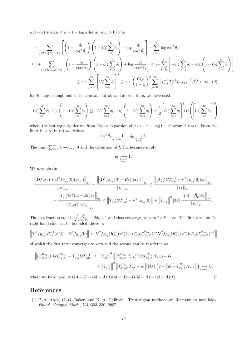
α(1− a) + log a ≤ α− 1− logα for all α, a > 0) into

−∑

j∈K∩{K,...,k}

(1− qj

cos2 θj

)1− Cζk∑i=j

δi

+ logqj

cos2 θj

− k∑j=K

log cos2 θj

≤ γ+∑

j∈{K,...,k}\K

(1− qj

cos2 θj

)1− Cζk∑i=j

δi

+ logqj

cos2 θj

≤ γ+

k∑j=K

−Cζ k∑i=j

δi − log

1− Cζk∑i=j

δi

≤ γ +

∞∑j=K

Cζ ∞∑i=j

δi

2

≤ γ +

(Cζb

1− β

)2 ∞∑j=K

∥∥T−1∗,j T−1j T∗,j+1

∥∥2 β2j <∞ (9)

for K large enough and γ the constant introduced above. Here, we have used

−Cζk∑i=j

δi−log

1− Cζk∑i=j

δi

≤ −Cζ ∞∑i=j

δi−log

1− Cζ∞∑i=j

δi

=1

2

Cζ ∞∑i=j

δi

2+OCζ ∞∑

i=j

δi

3

where the last equality derives from Taylor expansion of x 7→ −x − log(1 − x) around x = 0. From thelimit k →∞ in (9) we deduce

cos2 θk −→k→∞

1 , qk −→k→∞k∈K

1 .

The limit∑∞i=j δi →j→∞ 0 and the definition of K furthermore imply

qk −→k→∞k/∈K

1 .

We now obtain∥∥∥Df(xk) + D2fRxk (0)(pk, ·)∥∥∥xk

‖pk‖xk=

∥∥∥(D2fRxk (0)−Bk)(sk, ·)∥∥∥xk

‖sk‖xk≤

∥∥∥(T−∗∗,kGT−1∗,k −∇2fRxk(0))sk

∥∥∥xk

‖sk‖xk

+

∥∥∥T−∗∗,kG 12 (id− Bk)sk

∥∥∥xk∥∥∥T∗,kG− 1

2 sk

∥∥∥xk

≤∥∥∥T−∗∗,kGT−1∗,k −∇2fRxk(0)

∥∥∥ +∥∥∥T−1∗,k∥∥∥2 ‖G‖

∥∥∥(id− Bk)sk

∥∥∥x∗

‖sk‖x∗.

The last fraction equals√

q2kcos2 θk

− 2qk + 1 and thus converges to zero for k →∞. The first term on the

right-hand side can be bounded above by∥∥∥∇2fRxk(R−1xk

(x∗))−∇2fRxk(0)∥∥∥+

∥∥∥∇2fRxk(R−1xk

(x∗))− (T∗,kTRxkxk,x∗

)−∗∇2fRxk(R−1xk

(x∗))(T∗,kTRxkxk,x∗

)−1∥∥∥

of which the first term converges to zero and the second can be rewritten as∥∥∥(TRxkxk,x∗

)∗GTRxkxk,x∗

− T−∗∗,kGT−1∗,k

∥∥∥ ≤ ∥∥∥T−1∗,k∥∥∥2 ∥∥∥(TRxkxk,x∗

T∗,k)∗G(TRxkxk,x∗

T∗,k)−G∥∥∥

≤∥∥∥T−1∗,k∥∥∥2 ∥∥∥TRxkxk,x∗

T∗,k − id∥∥∥ ‖G‖ (2 +

∥∥∥id− TRxkxk,x∗T∗,k

∥∥∥) −→k→∞

0 ,

where we have used A∗GA−G = (id−A)∗G(id−A)−G(id−A)− (id−A)∗G.

References

[1] P.-A. Absil, C. G. Baker, and K. A. Gallivan. Trust-region methods on Riemannian manifolds.Found. Comput. Math., 7(3):303–330, 2007.

25

[2] P.-A. Absil, R. Mahony, and R. Sepulchre. Optimization algorithms on matrix manifolds. PrincetonUniversity Press, Princeton, NJ, 2008.

[3] P.-A. Absil, R. Mahony, and R. Sepulchre. Optimization on manifolds: Methods and with ap-plications. In Recent Advances in Optimization and its Applications in Engineering. The 14thBelgian-French-German Conference on Optimization, pages 125–144. Springer, 2010.

[4] Roy L. Adler, Jean-Pierre Dedieu, Joseph Y. Margulies, Marco Martens, and Mike Shub. Newton’smethod on Riemannian manifolds and a geometric model for the human spine. IMA J. Numer.Anal., 22(3):359–390, 2002.

[5] C. G. Baker, P.-A. Absil, and K. A. Gallivan. An implicit trust-region method on Riemannianmanifolds. IMA J. Numer. Anal., 28(4):665–689, 2008.

[6] Christopher G. Baker. Riemannian manifold trust-region methods with applications ot eigenprob-lems. PhD thesis, Florida State Universtity, 2008.

[7] Ian Brace and Jonathan H. Manton. An improved BFGS-on-manifold algorithm for computingweighted low rank approximations. In Proceedings of the 17th International Symposium on Mathe-matical Theory of Networks and Systems, pages 1735–1738, 2006.

[8] T. F. Chan and L. A. Vese. Active contours without edges. IEEE Transactions on Image Processing,10(2):266–277, 2001.

[9] D. Gabay. Minimizing a differentiable function over a differential manifold. J. Optim. Theory Appl.,37(2):177–219, 1982.

[10] Philipp Harms and Andrea Mennucci. Geodesics in infinite dimensional Stiefel and Grassmannmanifolds. 2010. submitted.

[11] Knut Huper and Jochen Trumpf. Newton-like methods for numerical optimization on manifolds. InConference Record of the Thirty-Eighth Asilomar Conference on Signals, Systems and Computers,volume 1, pages 136–139. IEEE, 2004.

[12] Huibo Ji. Optimization approaches on smooth manifolds. PhD thesis, Australian National University,2007.

[13] Martin Kilian, Niloy J. Mitra, and Helmut Pottmann. Geometric modeling in shape space. In ACMTransactions on Graphics, volume 26, pages #64, 1–8, 2007.

[14] Wilhelm P. A. Klingenberg. Riemannian geometry, volume 1 of de Gruyter Studies in Mathematics.Walter de Gruyter & Co., Berlin, second edition, 1995.

[15] Peter W. Michor and David Mumford. Riemannian geometries on spaces of plane curves. J. Eur.Math. Soc. (JEMS), 8(1):1–48, 2006.

[16] Jorge Nocedal and Stephen J. Wright. Numerical optimization. Springer Series in OperationsResearch and Financial Engineering. Springer, New York, second edition, 2006.

[17] Elijah Polak. Optimization, volume 124 of Applied Mathematical Sciences. Springer-Verlag, NewYork, 1997. Algorithms and consistent approximations.

[18] Chunhong Qi, Kyle A. Gallivan, and P.-A. Absil. Riemannian BFGS algorithm with applications.In Recent Advances in Optimization and its Applications in Engineering. The 14th Belgian-French-German Conference on Optimization, pages 183–192. Springer, 2010.

[19] Ekkehard W. Sachs. Broyden’s method in Hilbert space. Math. Programming, 35(1):71–82, 1986.

[20] Barry Simon. Trace ideals and their applications, volume 120 of Mathematical Surveys and Mono-graphs. American Mathematical Society, Providence, RI, second edition, 2005.

[21] S. T. Smith. Optimization techniques on Riemannian manifolds. Fields Institute Communications,3:113–135, 1994.

26

[22] G. Sundaramoorthi, A.C.G. Mennucci, S. Soatto, and A. Yezzi. A new geometric metric in thespace of curves, and applications to tracking deforming objects by prediction and filtering. SIAMJournal on Imaging Sciences, 2010. accepted.

[23] Constantin Udriste. Convex functions and optimization methods on Riemannian manifolds, volume297 of Mathematics and its Applications. Kluwer Academic Publishers Group, Dordrecht, 1994.

[24] Benedikt Wirth, Leah Bar, Martin Rumpf, and Guillermo Sapiro. A continuum mechanical approachto geodesics in shape space. International Journal of Computer Vision, 93:293–318, 2011.

[25] Y. Yang. Globally convergent optimization algorithms on Riemannian manifolds: uniform frameworkfor unconstrained and constrained optimization. J. Optim. Theory Appl., 132(2):245–265, 2007.

[26] Laurent Younes, Peter W. Michor, Jayant Shah, and David Mumford. A metric on shape space withexplicit geodesics. Atti Accad. Naz. Lincei Cl. Sci. Fis. Mat. Natur. Rend. Lincei (9) Mat. Appl.,19(1):25–57, 2008.

27