Optimization Methods for Piecewise A ne Model Fitting · Politecnico di Milano V Facolt a di...
113
Politecnico di Milano V Facolt` a di Ingegneria Corso di Laurea Specialistica in Ingegneria Informatica Optimization Methods for Piecewise Affine Model Fitting Tesi di Laurea Specialistica di Leonardo Taccari Relatore: Prof. Edoardo Amaldi Correlatore: Ing. Stefano Coniglio Anno Accademico 2009/2010
Transcript of Optimization Methods for Piecewise A ne Model Fitting · Politecnico di Milano V Facolt a di...

Politecnico di MilanoV Facolta di Ingegneria
Corso di Laurea Specialistica in
Ingegneria Informatica
Optimization Methods forPiecewise Affine Model Fitting
Tesi di Laurea Specialistica di
Leonardo Taccari
Relatore:
Prof. Edoardo Amaldi
Correlatore:
Ing. Stefano Coniglio
Anno Accademico 2009/2010

Contents
1 Introduction 6
1.1 Classical approach . . . . . . . . . . . . . . . . . . . . . . . . 8
1.2 Novelty of our approach . . . . . . . . . . . . . . . . . . . . . 10
1.3 k-Piecewise Affine Model Fitting . . . . . . . . . . . . . . . . 12
1.4 Subproblems . . . . . . . . . . . . . . . . . . . . . . . . . . . . 14
1.4.1 Hyperplane Clustering . . . . . . . . . . . . . . . . . . 15
1.4.2 Hyperplane Clustering and Piecewise Affine Model Fit-
ting . . . . . . . . . . . . . . . . . . . . . . . . . . . . 17
1.4.3 Classification . . . . . . . . . . . . . . . . . . . . . . . 21
1.4.4 Multi-category Classification: M-RLP . . . . . . . . . . 23
2 Exact MILP formulations for k-PAMF 29
2.1 Mixed integer formulation . . . . . . . . . . . . . . . . . . . . 30
2.1.1 Issues of the formulation . . . . . . . . . . . . . . . . . 34
2.2 Symmetry breaking techniques . . . . . . . . . . . . . . . . . . 35
2.2.1 Lexicographic ordering . . . . . . . . . . . . . . . . . . 37
2.2.2 Orbitopes: notation and definitions . . . . . . . . . . . 39
2.2.3 Shifted Column Inequalities . . . . . . . . . . . . . . . 41
2.2.4 Separation algorithm for SCIs . . . . . . . . . . . . . . 43
2.2.5 Extended formulation for orbitopes . . . . . . . . . . . 44

Contents ii
2.3 Dealing with Big-M . . . . . . . . . . . . . . . . . . . . . . . 47
2.3.1 Introduction to Combinatorial Benders’ Cuts . . . . . . 48
2.3.2 Combinatorial Benders’ Cuts for k-PAMF . . . . . . . 49
2.3.3 Irreducible Infeasible Subsystems . . . . . . . . . . . . 52
3 Heuristics 56
3.1 Three-Step PAMF Heuristic . . . . . . . . . . . . . . . . . . . 56
3.1.1 k-Plane Clustering . . . . . . . . . . . . . . . . . . . . 57
3.1.2 3-PAMF . . . . . . . . . . . . . . . . . . . . . . . . . . 58
3.1.3 Algorithm analysis . . . . . . . . . . . . . . . . . . . . 60
3.1.4 Complexity . . . . . . . . . . . . . . . . . . . . . . . . 61
3.1.5 Multi-start . . . . . . . . . . . . . . . . . . . . . . . . . 62
3.1.6 3-PAMF Variants . . . . . . . . . . . . . . . . . . . . . 63
3.2 Adaptive Point-Reassignment Heuristic . . . . . . . . . . . . . 66
3.2.1 PR-Local Search . . . . . . . . . . . . . . . . . . . . . 67
3.2.2 Adaptive Metaheuristic . . . . . . . . . . . . . . . . . . 70
3.2.3 APR Variant . . . . . . . . . . . . . . . . . . . . . . . 71
4 Computational results 72
4.1 Instances . . . . . . . . . . . . . . . . . . . . . . . . . . . . . . 72
4.1.1 Wave . . . . . . . . . . . . . . . . . . . . . . . . . . . . 72
4.1.2 Semi-random . . . . . . . . . . . . . . . . . . . . . . . 73
4.1.3 Noncontinuous regression . . . . . . . . . . . . . . . . . 73
4.2 Exact formulations . . . . . . . . . . . . . . . . . . . . . . . . 75
4.2.1 Implementation of symmetry breaking techniques . . . 75
4.2.2 Symmetry detection in CPLEX . . . . . . . . . . . . . 75
4.2.3 Choice of big-M . . . . . . . . . . . . . . . . . . . . . . 76
4.2.4 Remarks about notation . . . . . . . . . . . . . . . . . 76

Contents iii
4.2.5 Exact formulations on wave instances . . . . . . . . . . 77
4.2.6 Exact formulations on semi-random instances . . . . . 78
4.2.7 Exact formulations on nc-r instances . . . . . . . . . . 79
4.2.8 Implementation of CBC procedure . . . . . . . . . . . 80
4.2.9 Combining CBC and SCI . . . . . . . . . . . . . . . . 81
4.3 Heuristics . . . . . . . . . . . . . . . . . . . . . . . . . . . . . 82
4.3.1 Implementation . . . . . . . . . . . . . . . . . . . . . . 82
4.3.2 3-PAMF vs classic approach . . . . . . . . . . . . . . . 82
4.3.3 Heuristics on wave instances . . . . . . . . . . . . . . . 84
4.3.4 Heuristics on semi-random instances . . . . . . . . . . 85
4.3.5 Heuristics on nc-r instances . . . . . . . . . . . . . . . 86
4.4 Comparison of heuristic variants . . . . . . . . . . . . . . . . . 89
4.4.1 3-PAMF variants . . . . . . . . . . . . . . . . . . . . . 89
4.4.2 APR Variants . . . . . . . . . . . . . . . . . . . . . . . 94
4.5 UCI Machine Learning Instances . . . . . . . . . . . . . . . . 95
4.5.1 WPBC . . . . . . . . . . . . . . . . . . . . . . . . . . . 95
4.5.2 Machine-CPU . . . . . . . . . . . . . . . . . . . . . . . 95
5 Concluding remarks 97
A SCI separation algorithm 99
B Code 102

Abstract
Given numerical data sampled from a real, unknown process the problem of
Model Fitting is to find a model that best fits the data, i.e., a mathematical
function which is able to approximate the data as accurately as possible.
In this work we investigate Piecewise Affine Models, which are attracting
considerable attention in a variety of fields. A Piecewise Affine Model is
described by k affine functions each one associated to a subdomain Dj ⊆ Rn,
with 1 ≤ j ≤ k, where {D1, ...,Dk} is a partition of Rn. The problem of
k-Piecewise Affine Model Fitting (k-PAMF) amounts to identifying k linear
submodels fj : Dj → R, together with their definition domains Dj, so as to
minimize an objective function which represents the overall approximation
error with respect to the data.
Typically the problem is solved in two distinct phases. In the first phase
the data points are partitioned in k subsets and a linear submodel is fitted to
each subset, while in the second phase the subdomains Dj are defined. We
propose a novel approach that combines the two aspects in a single phase.
The thesis is organized as follows. In Chapter 1 we give an overview of
previous work on the subject and explain the novelty of our approach. The
problem of k-PAMF is described in detail and the subproblems Hyperplane
Clustering and Multi-category Classification are discussed. In Chapter 2 we

Abstract 2
propose a novel Mixed-Integer Linear Programming formulation for k-PAMF.
We describe the generation of ad-hoc cuts in a Branch&Cut framework to
break symmetries and speed up the solution time. Moreover, we use a Com-
binatorial Benders’ Cuts approach to get rid of the big-M coefficients. In
Chapter 3 we propose two heuristics to tackle large-size instances: an adap-
tation of k-means and an adaptive point reassignment algorithm. In Chapter
4 we report and discuss computational results obtained from randomly gen-
erated and real-world instances, and we compare the methods we propose.
The refined exact formulations yield optimal solutions for instances up to
150 points in low-dimensional spaces while the adaptive point reassignment
method provides good solutions in a short computing time. Finally, in Chap-
ter 5 we draw some conclusions and mention ideas for future work.

Riassunto
Nel problema del Model Fitting, dato un insieme A di punti ai ∈ Rn e i
loro cosiddetti valori osservati yi ∈ R, si vuole identificare un modello, cioe
una funzione f : D ⊆ Rn → R, che approssimi nel miglior modo possibile il
processo reale f(·) che ha generato i dati yi.
In questa tesi si studia il problema di k-Piecewise Affine Model Fitting, che
prevede l’approssimazione di funzioni non lineari con modelli lineari (affini)
a tratti. Il problema e di attuale rilevanza in molti ambiti applicativi, ad
esempio nei modelli Piecewise AutoRegressive eXogenous (PWARX).
Un modello f lineare a tratti (in generale non continuo) e descritto da un
numero k di funzioni lineari ciascuna delle quali e associata ad un proprio
dominio Dj ⊆ Rn. Il problema di k-PAMF consiste nel trovare k sottomodelli
affini fj : Dj → R che minimizzano una funzione obiettivo che rappresenta
l’errore di approssimazione sui dati. Una tipica funzione che viene usata allo
scopo e la somma dei moduli delle differenze fra le osservazioni yi e il valore
calcolato dal modello:∑m
i=1 |fj(ai) − yi|p, dove fj e il sottomodello lineare
nel cui dominio giace il punto ai. La scelta nel nostro caso e la norma `1,
p = 1, ovvero la minimizzazione della somma dei valore assoluti degli errori
di approssimazione per ogni punto.
Il problema da risolvere comprende non solo la stima dei parametri dei
sottomodelli lineari, ma anche l’identificazione dei loro domini Dj. Cio che

Riassunto 4
viene tipicamente fatto nell’approccio classico e dividere il problema in due
fasi: nella prima vengono partizionati i punti e si trovano gli iperpiani che
meglio approssimano tali sottoinsiemi di punti, mentre la determinazione dei
domini dei sottomodelli lineari viene svolta solamente in seconda battuta.
L’approccio che proponiamo in questo lavoro prevede un’unica formulazione
che contemporaneamente lavora sulla minimizzazione dell’errore sui dati e
sulla partizione del dominio continuo in k regioni corrispondenti ai sotto-
modelli lineari.
Nel Capitolo 1 e descritto il problema di k-Piecewise Affine Model Fit-
ting con rimandi a precedenti lavori sull’argomento, mostrando la novita
dell’approccio proposto. Inoltre vengono introdotti due problemi ad esso
collegati, l’Hyperplane Clustering e la Multi-category Classification. In ef-
fetti k-PAMF puo essere visto come una loro combinazione. Nel Capitolo
2 viene presentata una formulazione esatta di k-PAMF come un problema
di programmazione lineare misto-intera. Esso prevede allo stesso tempo la
detereminazione dei parametri e dei domini dei modelli lineari. Descriviamo
lo studio e l’implementazione di metodi che cercano di ridurre la complessita
del problema affrontando due aspetti critici della formulazione: le simme-
trie e i big-M . Nel primo caso consideriamo la generazione di una classe di
tagli che permettono la rottura delle simmetrie con un netto miglioramento
dell’efficienza. Nel secondo caso evitiamo l’utilizzo dei coefficienti big-M
medienta una decomposizione basata sui Combinatorial Benders’ Cuts. Nel
Capitolo 3 sono proposte due euristiche: una procedura iterativa simile a
k-means ed un algoritmo che e basato sull’individuazione di punti candidati
ad essere riassegnati. Entrambi gli algoritmi, che prevedono diverse varianti,
forniscono delle soluzioni (subottimali) di buona qualita in tempi brevi. Il
Capitolo 4 riporta e discute i test computazionali che sono stati effettuati su

Riassunto 5
istanze reali e generate aleatoriamente. Infine, nel Capitolo 5 sono contenute
delle conclusioni ed alcuni sviluppi futuri.

Chapter 1
Introduction
Given a set A of m points ai ∈ Rn and their corresponding observations
f(ai) = yi ∈ R, where f(·) is an unknown, possibly nonlinear, function, the
problem of Model Fitting is to find a mathematical function f(·) which best
approximates the unknown function by minimizing the error on the data
points.
The fundamental issue of Model Fitting is the choice of the model and its
complexity. Typically real-world data exhibit nonlinearties and are affected
by errors (see Figure 1.1). A model which is too simple (e.g., affine models)
might lack the ability to extract all the information provided by the data. On
the other hand, a model which is too involved might be too complicated to use
efficiently or overfit the data (e.g., reproduce even noise). This is consistent
with Occam’s principle, which states that, when a choice is possible, the
simplest model has to be preferred.
In this work we investigate Piecewise Affine Models, also called Piecewise
Linear Models. The choice of piecewise affine models is motivated by the
difficulty that lies in the identification and the use of nonlinear models. While
basic affine models are often too simple to cope with the actual complexity

Chapter 1. Introduction 7
of real data, piecewise affine functions are considered to be general enough
to work well in practice, while maintaining most of the practical advantages
given by linear models.
0
0.1
0.2
0.3
0.4
0.5
0.6
0.7
0 0.2 0.4 0.6 0.8 1
Figure 1.1: A set of points that exhibit highly nonlinear behaviour and canbe fitted accurately with 3 affine submodels.
The Piecewise Affine Model Fitting problem requires to find a model
f : D ⊆ Rn → R, composed by a given number k of affine submodels fj such
that the overall approximation error is minimized. Each affine submodel
fj : Dj → R, for j = 1 . . . k, is described by a linear function fj(x) =
wTj x− γj and a definition domain Dj ⊆ D: in each region one would like to
identify a hyperplane that best fits the data. We impose no constraints on
the continuity of the model. An example of piecewise linear noncontinuous
model is reported in Figure (1.2).
If the partitioning of the domain is known a priori, i.e., the definition
domains of the submodels are known, the problem can be reduced to a fixed
number of linear model fitting problems, which can be easily solved with
robust regression techniques. This however requires some deep knowledge of
the function that we are approximating, and it is not always the case. Indeed,

Chapter 1. Introduction 8
−1
0
1
−1
−0.5
0
1−10
−5
0
5
10
0.5
1−10
−5
0
5
10
Figure 1.2: A piecewise linear discontinuous model with 3 submodels.
it is likely that we just have an indication of the number of submodels k.
Often we might have no a priori knowledge that can help in the model fitting
process, thus both the number of the linear submodels and their definition
domains Dj (a polyhedral partition of the continuous domain D) have to be
completely identified from the raw data.
1.1 Classical approach
The problem of Piecewise Affine Model Fitting arises in a variety of fields, and
a number of different methods exist. Classical techniques typically work in
two phases. The first phase involves partitioning and fitting the data points:
the algorithm looks for coplanarity in the discrete space of the data points.
Then, in a second phase, the definition regions Dj of the affine submodels
are derived. However, the affine subspaces that have been found in the first
phase might not induce a feasible partition on the continuous domain D:
some points might therefore be assigned to a subdomain Dj that is different

Chapter 1. Introduction 9
from the one that corresponds to the submodel they contributed to define.
An example is reported in Figure 1.3. This is a flaw that our novel approach
aims to repair (see Section 1.2).
Figure 1.3: Example showing two intersecting linear submodels. Accordingto the point-hyperplane y-distance, the black point would be assigned to thesubmodel on the left. However, the resulting sets are not linearly separablein the continuous domain (the x-axis), hence we would like the black pointto be assigned to the submodel on the right.
In the context of system identification the problem is usually referred to as
hybrid system estimation, and the models are called Piecewise AutoRegres-
sive eXogenous (PWARX) models. An overview of a number of techniques
for hybrid systems identification is proposed in [PJFTV07], that contains
references to several works on Piecewise Affine Model Fitting. Identification
procedures described in the paper include an algebraic approach, a Bayesian
procedure and a clustering-based method. The continuous domain partition
is achieved in a second phase by means of multi-category classification, that is
performed with Support Vector Machines (SVM, [Vap98]) or Robust Linear
Programming (RLP, [BB99]).
In [AM02] the authors tackle piecewise linear model fitting as a Min-
PFS problem, which requires to find a partition of a given linear system in a

Chapter 1. Introduction 10
minimum number of feasible subsystems (with a maximum noise tolerance ε).
The problem isNP-hard, and an effective greedy algorithm is proposed in the
paper. The method does not account for the continuous domain partition: in
[BGPV03] the authors introduce a second phase that derives the subdomains
via multicategory classification, performed with SVM or RLP.
In [FTMLM03] the data points are first clustered in feature space via
k-means and then the parameters for each model are computed. The par-
tition is derived at a later stage via SVM or RLP. In [FTM02] the fitting
is performed with a 3-layers neural network which models a piecewise linear
function. The subdomains are not explicitly derived. [MB09] use an iterative
algorithm for estimating max-affine models: even in this case the domains
of the submodels are not explicit, as a linear model is active in a region if it
is maximal compared to the other ones. The resulting piecewise model is, by
definition, continuous, while our formulation is more general since the model
can be discontinuous.
1.2 Novelty of our approach
In this thesis we propose a novel approach that follows in the footsteps of
the work in [CI06], where a single-phase formulation for k-Piecewise Linear
Model Fitting is introduced. What distinguishes this approach from most
of the previous work on the subject is the fact that we do not focus first on
fitting discrete points, then on determining the domains of the submodels.
On the contrary, we attempt to solve both problems simultaneously.
The drawbacks of previous, two-phase, approaches are evident especially
in cases where distinct submodels are almost coplanar, or when we have
intersecting submodels. As an example we display in Figure 1.4 a small
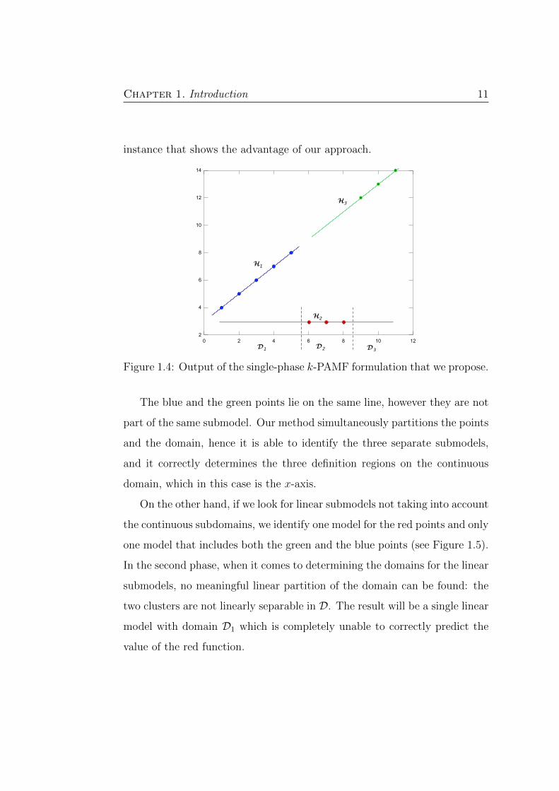
Chapter 1. Introduction 11
instance that shows the advantage of our approach.
2
4
6
8
10
12
14
0 2 4 6 8 10 12
H1
H2
H3
D1 D2 D3
Figure 1.4: Output of the single-phase k-PAMF formulation that we propose.
The blue and the green points lie on the same line, however they are not
part of the same submodel. Our method simultaneously partitions the points
and the domain, hence it is able to identify the three separate submodels,
and it correctly determines the three definition regions on the continuous
domain, which in this case is the x-axis.
On the other hand, if we look for linear submodels not taking into account
the continuous subdomains, we identify one model for the red points and only
one model that includes both the green and the blue points (see Figure 1.5).
In the second phase, when it comes to determining the domains for the linear
submodels, no meaningful linear partition of the domain can be found: the
two clusters are not linearly separable in D. The result will be a single linear
model with domain D1 which is completely unable to correctly predict the
value of the red function.

Chapter 1. Introduction 12
2
4
6
8
10
12
14
0 2 4 6 8 10 12
D1
H1
H2
Figure 1.5: Output of a classical k-PAMF method working in two distinctphases. It is unable to induce suitable definition regions for the submodels.All points are considered part of the domain of H1.
1.3 k-Piecewise Affine Model Fitting
Let A be a set of m points ai ∈ Rn and f(ai) = yi ∈ R the observations
associated to the points ai, where f(·) is an unknown nonlinear function.
The problem of k-Piecewise Affine Model Fitting amounts to finding a model
f : D ⊆ Rn → R, composed by a given number k of linear submodels fj such
that the overall approximation error is minimized. For each affine submodel
it is necessary to identify a linear function fj(x) = wTj x−γj and a definition
domain Dj ⊆ D.
To have a formal mathematical formulation for k-PAMF we have to in-
troduce a metric to measure the discrepancy between the model and the data
values. Typically this objective function is defined as a norm of the vector
containing the approximation errors for each point, i.e., a function of the
form:m∑i=1
|fj(i)(ai)− yi|p,

Chapter 1. Introduction 13
where j(i) indicates the index of the submodel in whose domain the data
point lies.
In this work we define the objective function of k-PAMF as:
m∑i=1
|fj(i)(ai)− yi|, (1.1)
taking p = 1, that is the sum of the absolute values of the approximation
errors. In other words, the error function for the problem is expressed in
terms of the norm `1 of the vector containing the approximation errors: this
translates easily into a linear mathematical program. Moreover with `1 we
expect the formulation to be less sensitive to outliers than using a norm with
p > 1, like the `2 norm.
According to this definition of the problem it is possible to derive a first
nonlinear mathematical formulation for k-PAMF:
mink∑j=1
m∑i=1
xijdij (1.2)
∑j
xij = 1 ∀i ∈ [m] (1.3)
dij = |fj(ai)− yi| ∀i ∈ [m], j ∈ [k] (1.4)
fj(ai) = wTj ai − γj ∀i ∈ [m], j ∈ [k] (1.5)
xij = 1⇔ ai ∈ Dj ∀i ∈ [m], j ∈ [k] (1.6)
xij ∈ {0, 1} ∀i ∈ [m], j ∈ [k] (1.7)
dij, γj ∈ R ∀i ∈ [m], j ∈ [k] (1.8)
wj ∈ Rn ∀j ∈ [k] (1.9)
k⋃j=1
Dj = D, Dj ∩ Dl = ∅ ∀j 6= l (1.10)

Chapter 1. Introduction 14
The binary variables xij indicate whether the point i is assigned to the
model j. Hence the objective function accounts for the approximation error
dij only if xij has value 1, since we are not interested in the error regarding the
submodels where a point does not belong. It is important to stress that the
subdomainsDj are not fixed: they have to be derived so that a point ai can be
assigned to a submodel fj only if it belongs to Dj. Constraints (1.10) ensure
that the subdomains are a partition of D, i.e., they are disjoint and their
union forms D. In this formulation it is still not explicit how the domains Djshould be treated in practice. Mixed-Integer Linear Programming (MILP)
formulations for the problem are the object of Chapter 2.
1.4 Subproblems
Piecewise Affine Model Fitting can be seen as the combination of three dif-
ferent subproblems.
In the first subproblem, which is combinatorial, the points have to be
partitioned so that each one is assigned to one (and only one) linear submodel,
as expressed by the binary assignment variables xij.
In the second subproblem, which is continuous, the hyperplanes parame-
ters (wj, γj) have to be determined such that they minimize the sum of the
absolute errors between the predicted values fj(ai) and the observations yj
in each data point ai.
Together these two subproblems form a variant of what is called k-
Hyperplane Clustering [ACD09].
In the third subproblem the domain D has to be partitioned so that each
point belongs to the domain Dj corresponding to the submodel fj(·) it is
assigned to. This can be seen as a multi-category classification problem,

Chapter 1. Introduction 15
that is to find a discriminating function that induces a polyhedral partition
on the continuous domain D which is consistent with the assignments of the
data points to the submodels.
In the next sections we describe in detail the Hyperplane Clustering prob-
lem and the Multi-category Classification problem.
1.4.1 Hyperplane Clustering
Clustering is the problem of discovering clusters, or groups, of similar el-
ements in a dataset. Similarity in itself is a rather vague term, hence the
problem can be defined, and thus solved, in many different ways. Usually
two points are considered similar according to a metric defined on the space
they lie in, e.g., the Euclidean distance. The desired result of a clustering
process is generally a minimal number k of clusters with high infra-cluster
and low inter-cluster similarity.
In Hyperplane Clustering the focus is not on the proximity between points
but on their collinearity (or coplanarity). This is to say that the aim is
clustering data such that elements of the same group are close to the same
linear subspace of dimension n− 1 (a hyperplane, hence the name). In other
words, given a set of m points A = {a1, a2, . . . , am} belonging to Rn, we seek
to determine a minimal number k of hyperplanes
Hj = {x ∈ Rn|wTj x = γj,wj ∈ Rn, γj ∈ R} (1.11)
and an assignment of the points of A to the hyperplanes Hj such that the
resulting clusters minimize an overall error (an objective function) which
depends on the aggregated orthogonal distance between the points and their
corresponding hyperplanes (see Figure 1.6). For a comprehensive discussion

Chapter 1. Introduction 16
Figure 1.6: In kHC we look for a number k of hyperplanes that minimize thesum of the square orthogonal point-hyperplane distances.
on most aspects of the problem see [ACD09].
A MILP formulation of Hyperplane Clustering with a fixed number k of
clusters (k-HC) is the following:
mink∑j=1
m∑i=1
xijdij (1.12)
∑j
xij = 1 ∀i ∈ [m] (1.13)
dij =|wT
j ai − γj|‖wj‖2
∀i ∈ [m], j ∈ [k] (1.14)
xij ∈ {0, 1} ∀i ∈ [m], j ∈ [k] (1.15)
wj ∈ Rn ∀j ∈ [k] (1.16)
dij, γj ∈ R ∀i ∈ [m], j ∈ [k] (1.17)
This formulation adopts a 2-norm distance:
dij =|wT
j ai − γj|‖wj‖2
. (1.18)

Chapter 1. Introduction 17
and an objective function that takes into account for each cluster the sum of
all point-hyperplane distances. The binary variables xij have value 1 when
the point ai is assigned to the cluster j and 0 otherwise. It is necessary
to point out that this formulation is rather naive, as it involves many non-
linearties that could be avoided or reformulated in a form better suited for
mathematical programming.
1.4.2 Hyperplane Clustering and Piecewise Affine Model
Fitting
The similarities between Piecewise Affine Model Fitting and Hyperplane
Clustering are many and not difficult to see, since both require to partition
the data and to identify k hyperplanes.
An important difference between the PAMF and HC lies in the objective
function. In Hyperplane Clustering the aim is of minimizing an aggregate
distance function which depends on the orthogonal distance of the points
from the hyperplanes,
di =|wT
j(i)ai − γj(i)|‖wj(i)‖2
. (1.19)
In PAMF, on the contrary, we seek the minimum sum of the absolute values
of the residuals∑
i |εi|, where εi is defined as the difference between the
observed value yi and the estimated value fj(i)(xi) = wTj(i)xi−γj(i). Formally:
εi := fj(i)(ai)− yi = wTj(i)ai − γj(i) − yi. (1.20)
In both cases j(i) identifies the cluster that ai has been assigned to. Figure
1.7 shows the difference between the distance functions of the two problems.
By replacing the objective function of (1.12)-(1.17) we can write a pro-

Chapter 1. Introduction 18
Figure 1.7: On the left we show a plane minimizing the orthogonal distanceof the blue points, but that does not translate in an optimal solution on they-axis (center). The plane on the right correctly minimizes the sum of theabsolute values of residuals.
gram which is very similar to k-PAMF, although it lacks the continuous
domain partitioning.
mink∑j=1
m∑i=1
xij dij (1.21)
∑j
xij = 1 ∀i ∈ [m] (1.22)
dij = |wTj ai − γj − yj| (1.23)
xij ∈ {0, 1} (1.24)
We can work to write it in a better form. This program can be rephrased as
a Mixed-Integer Linear Programming (MILP) problem removing all nonlin-
earities, first by noticing that the objective function can be written as:
mink∑j=1
m∑i=1
dij (1.25)

Chapter 1. Introduction 19
with the additional implications
xij = 0⇒ dij = 0 (1.26)
xij = 1⇒ dij = |wTj ai − γj − yj| (1.27)
thus making the objective linear. Now the conditional constraints can be
easily transformed in linear constraints using the well known big-M technique
(see Section 2.3 for a discussion on it). Then we can remove the absolute
norm by introducing two sets of linear inequalities
dij ≥ wTj ai − γj − yj (1.28)
dij ≥ −wTj ai + γj + yj (1.29)
which are equivalent to the original equations provided that we are dealing
with a minimization problem. The resulting MILP problem is the following,
where for convenience we introduce the auxiliary variables dij:

Chapter 1. Introduction 20
mink∑j=1
m∑i=1
dij (1.30)
∑j
xij = 1 ∀i ∈ [m] (1.31)
dij ≤Mxij ∀i ∈ [m], j ∈ [k] (1.32)
dij ≥ dij −M(1− xij) ∀i ∈ [m], j ∈ [k] (1.33)
dij ≥ wTj ai − γj − yj ∀i ∈ [m], j ∈ [k] (1.34)
dij ≥ −wTj ai + γj + yj ∀i ∈ [m], j ∈ [k] (1.35)
xij ∈ {0, 1} ∀i ∈ [m], j ∈ [k] (1.36)
wj ∈ Rn ∀j ∈ [k] (1.37)
dij, γj ∈ R ∀i ∈ [m], j ∈ [k] (1.38)
For a pair (i, j), given a sufficiently large value of M , when xij = 0 the
Inequality (1.32) is active and dij is bound to be 0. Viceversa, if xij = 1 the
Constraint (1.33) has to be satisfied (dij ≥ dij).
This is a MILP which is very closely related to k-PAMF, yet it is not
enough to fully express the problem. In PAMF we intend not only to parti-
tion the given discrete dataset A, but also to guarantee that the partitioned
points be linearly separable and to compute a partition of the continuous
domain D. This is done by adding classification constraints with the pur-
pose of linearly separating the data and at the same time determining the
k subdomains where the linear submodels are defined. Such constraints are
meant to avoid the point-cluster assignments which would not translate into
a feasible linear partition of the underlying domain D. The partition of D
can be achieved through multi-category linear classification, as in [CI06], that

Chapter 1. Introduction 21
will be discussed in the next section.
1.4.3 Classification
Given two sets of points A1,A2 in the n-dimensional space Rn, classification
is the problem of identifying a function capable of discriminating the data
according to their classes.
If a linear function is enough to discriminate the two classes, it is sufficient
to find an (n− 1)-dimensional hyperplane H defined as
H : wTx− γ = 0 (1.39)
where w is the normal to the plane and γ the distance from the origin, and
such that for each point ai it fulfils the constraints
wTai − γ > 0 if ai ∈ A1 (1.40)
wTai − γ < 0 if ai ∈ A2. (1.41)
If such a separating plane exists, the points are said to be linearly separable.
In this case in general there are infinitely many planes that separate the two
classes.
A common approach to deal with this problem in practice is introducing
the following nonomogeneous inequalities.
wTai − γ ≥ +1 if ai ∈ A1 (1.42)
wTai − γ ≤ −1 if ai ∈ A2 (1.43)
These constraints do not only define a hyperplane separating the data

Chapter 1. Introduction 22
Figure 1.8: A linear separation bound. The points on the margin ρ are thesupport vectors.
points, but in fact two parallel hyperplanes that keep a margin between the
points belonging to different classes. In particular, the distance between
the two hyperplanes is 2/‖w‖, that represents in fact the minimum distance
between two points belonging to different classes. The points lying on the hy-
perplanes that define the margin between the classes are called Support Vec-
tors (see Figure 1.8), and a well-known and powerful classification method,
called Support Vector Machines (SVM), is based on the maximization of the
geometric margin ρ = 2/‖w‖.
This technique requires a quadratic minimization problem, and the obvi-
ous drawback of this method is the potential complexity of the optimization.
Moreover, when dealing with sets which are not completely separable with
a linear function, it is important to find a result that discriminates best
according to some criterion other than the maximal separation margin. A
formulation that naturally accounts for misclassification errors and just re-
quires the solution a linear problem is Robust Linear Programming (RLP,

Chapter 1. Introduction 23
[BB99]):
minm∑i=1
ei (1.44)
wTai − γ + ei ≥ +1 if ai ∈ A1 (1.45)
wTai − γ − ei ≤ −1 if ai ∈ A2 (1.46)
w ∈ Rn, γ ∈ R (1.47)
ei ≥ 0 (1.48)
that amounts to minimizing the sum of the misclassification errors ei.
1.4.4 Multi-category Classification: M-RLP
What was described in the previous section is valid for a binary classification,
but can be extended to multi-class problems, where k > 2. Given k sets
A1, ...,Ak we want to find a classification function capable of discriminating
them.
A typical technique is subdividing the k-category classification problem
in k binary discrimination problems, i.e., for each set Ai the method builds a
function that discriminates that class from the remaining k − 1 (one-versus-
all). Then, when a new point has to be classified, k binary decisions have
to be made, and the highest output wins. This procedure has been vastly
adopted both in SVM and RLP contexts with the name k-SVM and k-RLP
[BB99].
These methods require the identification of a set of parameters (w1, γ1), . . .
(wk, γk) such that for each class Aj and for each ai ∈ Aj
wTj ai − γj > wT
l ai − γl ∀l ∈ [k], l 6= j (1.49)

Chapter 1. Introduction 24
w1x − 1
A1
A3A2
w2x −γ
2
w3x −
3
f(x)= maxi =1, 2, 3
w x−γi
γ γ
i
Figure 1.9: Example of a piecewise discriminating function for three classes.
A point ai is classified as belonging to Aj if the above inequalities hold. In
other words, the class of a point is determined by the index of the pair (wj, γj)
that maximizes the function fj(ai) = wTj ai − γj. Indeed, the discriminating
function can be expressed as the piecewise linear function (an example in
Figure 1.9):
g(x) = maxj∈[k]{xTwj − γj}
where the classification function is
c(x) = arg maxj∈[k]{xTwj − γj}.
The separating plane of a class Aj from a class Al can be defined as the
points satisfying
(wj −wl)Tx− (γj − γl) = 0, (1.50)
where the parameters are computed so that (wj −wl)Tai − γj + γl > 0 for
each points belonging to the set Aj and viceversa (wj −wl)Tai− γj + γl < 0
for each point in Al.

Chapter 1. Introduction 25
xT (w1 −w2) = γ1 −γ2
xT (w2 −w3) = γ2−γ3
xT (w3 −w1) = γ3 −γ1
A2
A3
A1
Figure 1.10: Example of a piecewise linear separator for three classes.
If the inequalities are perfectly satisfied, the sets of points are said to be
piecewise-linearly separable (Figure 1.10).
A different approach is proposed by Bennett and Mangasarian in [BM94].
The formulation introduced in the paper is a generalization of RLP called
M-RLP and requires only a single linear optimization in contrast to the k
problems of k-SVM and k-RLP. First we introduce the equivalent nonomo-
geneous inequalities
(wj −wl)Tai − γj + γl ≥ 1 (1.51)
for each point ai ∈ Aj and for all l 6= j. Accordingly to the proposed
inequalities, a point assigned to a class Aj is considered misclassified if there
exists an l 6= j such as (wj − wl)Tai − γj + γl − 1 ≤ 0. We can therefore
consider the negative quantity (wj−wl)Tai−γj+γl−1 as a misclassification
error, while, if positive, it measures the “strength” of the classification. It is
straightforward to define the misclassification error for ai ∈ Aj with respect

Chapter 1. Introduction 26
to Al as:
eijl = max{0,−(wj −wl)Tai + γj − γl + 1}, (1.52)
where we have inverted the sign of the expression to have a non-negative
quantity. The sum of the errors eijl is the quantity to be minimized in order
to find the separator which best discriminates between the two classes Aj and
Al. This can be generalized with an aggregate error function which accounts
for the misclassification errors of each point.
mink∑j=1
k∑l=1l 6=j
∑i:ai∈Aj
eijl (1.53)
eijl ≥ −(wj −wl)Tai + γj − γl + 1 ∀j, l 6= j ∈ [k], i : ai ∈ Aj (1.54)
eijl ≥ 0 ∀j, l ∈ [k], i : ai ∈ Aj (1.55)
wj ∈ Rn ∀j ∈ [k] (1.56)
eijl, γj ∈ R ∀j ∈ [k] (1.57)
If the optimal objective is 0, then the dataset is piecewise-linearly sepa-
rable. Otherwise, the positive values of the variables eijl represent the mag-
nitude of the misclassification error of the point ai.
M-RLP variant: max-error
In the context of this work a slightly different objective function has been
adopted. Working within a Piecewise Affine Model Fitting context, we are
often interested in setting a misclassification error tolerance rather than min-
imizing such errors. Moreover, as will be clear further on, the classification
will be made on classes that are not fixed a priori. We adopt a formulation

Chapter 1. Introduction 27
with a simpler objective function:
minm∑i=1
ei (1.58)
ei ≥ eijl ∀j, l ∈ [k], i : ai ∈ Aj (1.59)
eijl ≥ −(wj −wl)Tai + γj − γl + 1 ∀j, l 6= j ∈ [k], i : ai ∈ Aj (1.60)
ei ≥ 0 ∀i ∈ [m] (1.61)
eijl ≥ 0 ∀j, l ∈ [k], i : ai ∈ Aj (1.62)
wj ∈ Rn ∀j ∈ [k] (1.63)
γj ∈ R ∀j ∈ [k] (1.64)
This program amounts to minimizing the sum of the maximum misclassifi-
cation errors ei for each point ai rather then minimizing the sum of all the
misclassification errors for each point [CI06].
In this formulation the presence of the classification constraints depends
on the class labels of the points ai. As long as the sets Aj are known a
priori, as it is the case in a classic supervisioned learning problem, the sys-
tem of inequalities can be written easily. We now introduce a different, but
equivalent, formulation that is better suited for the use that will be made in
k-PAMF. We add a number m × k of binary parameters xij ∈ {0, 1} which
express the assignment of a point ai to the class Aj. These assignments have
to satisfy∑
j xij = 1 and allow us to declare Constraint (1.60) as:
xij = 1⇒ eijl ≥ −(wj −wl)Tai + γj − γl + 1 (1.65)
Again, we deal with the conditional constraint with the big-M method:

Chapter 1. Introduction 28
minm∑i=1
ei (1.66)
ei ≥ eijl −M(1− xij) ∀j, l ∈ [k], i ∈ [m] (1.67)
eijl ≥ −(wj −wl)Tai + γj − γl + 1 ∀j, l 6= j ∈ [k], i ∈ [m] (1.68)
ei ≥ 0 ∀i ∈ [m] (1.69)
eijl ≥ 0 ∀j, l ∈ [k], i ∈ [m] (1.70)
wj ∈ Rn ∀j ∈ [k] (1.71)
γj ∈ R ∀j ∈ [k] (1.72)
When xij = 0 inequality 1.67 is deactivated and ei assumes value 0. The
variable eijl is auxiliary and is used for readability purpose, but could be
omitted with a simple substitution obtaining:
ei ≥ −(wj −wl)Tai + γj − γl + 1−M(1− xij) (1.73)
The value of M is once again crucial, as it has to be big enough (ideally
+∞) but could cause numerical instabilities if too large.

Chapter 2
Exact MILP formulations for
k-PAMF
In this chapter we present a MILP formulation for k-PAMF which includes
not only clustering and linear regression on the data points, but also multi-
category classification that directly induce a partition on the domain D.
With our mixed-integer formulation it is possible to find a global optimum
to the Piecewise Affine Model Fitting problem with no previous information
on the unknown function f(·) that we want to approximate. The only pa-
rameter that the method requires is the number k of affine submodels.
The devised MILP program is hard to solve to optimality. We show
methods which exploit the peculiarities of the formulation and apply some
promising recent results from the literature to cope with the complexity of
the problem.

Chapter 2. Exact MILP formulations for k-PAMF 30
2.1 Mixed integer formulation
Our mixed integer formulation of k-PAMF combines all aspects of Piecewise
Affine Model Fitting in one single program. A first part of the formulation
follows from what has been discussed in Section 1.4.2 about Hyperplane
Clustering and how it is related to PAMF: we seek an assignment to the k
clusters such that the distance of each cluster member from the corresponding
model is minimal. In other words, we look for a partition of the discrete set
of points A in subsets associated to k submodels. The objective function
is the sum of the absolute values of the residuals, i.e., the difference dij
between the observed value yi of each point and the value fj(ai) given by
the affine submodel (hyperplane). In Section 1.4.2 we discussed the following
MILP, that is a modification of a k-HC program where we have replaced the
geometric `2-norm objective function with the `1-norm algebraic distance of

Chapter 2. Exact MILP formulations for k-PAMF 31
PAMF (which we repeat for greater readability):
mink∑j=1
m∑i=1
dij (2.1)
∑j
xij = 1 ∀i ∈ [m] (2.2)
dij ≤Mxij ∀i ∈ [m], j ∈ [k] (2.3)
dij ≥ dij −M(1− xij) ∀i ∈ [m], j ∈ [k] (2.4)
dij ≥ wTj ai − γj − yj ∀i ∈ [m], j ∈ [k] (2.5)
dij ≥ −wTj ai + γj + yj ∀i ∈ [m], j ∈ [k] (2.6)
xij ∈ {0, 1} ∀i ∈ [m], j ∈ [k] (2.7)
dij ≥ 0 ∀i ∈ [m], j ∈ [k] (2.8)
wj ∈ Rn ∀j ∈ [k] (2.9)
γj ∈ R ∀i ∈ [m], j ∈ [k] (2.10)
What is yet to be added is a second part which performs simultaneously
a multi-category classification on the continuous domain D based on the as-
signments xij – which are not fixed. What usually happens with supervised
learning is that we have points assigned to classes and we look for a sepa-
ration of the domain such as the points belonging to different categories are
accordingly classified. In contrast, in our formulation of k-PAMF we have a
shift of paradigm: we do have a classification problem, but the supervision
labels, or characteristic vectors, xij are not known a priori. Instead, they are
variables that assume a value according to the remaining constraints.
The M-RLP formulation chosen to be included in the k-PAMF program

Chapter 2. Exact MILP formulations for k-PAMF 32
is the following (see Section 1.4.4):
minm∑i=1
ei (2.11)
ei ≥ eijl −M(1− xij) ∀j, l ∈ [k], i ∈ [m] (2.12)
eijl ≥ −(wj −wl)Tai + γj − γl + 1 ∀j, l 6= j ∈ [k], i ∈ [m] (2.13)
ei ≥ 0 ∀i ∈ [m] (2.14)
eijl ≥ 0 ∀j, l ∈ [k], i ∈ [m] (2.15)
which is convenient because it is straightforward to change the role of the
characteristic vectors xi from parameters to binary variables. We replace the
minimization term with a tolerance η on each ei, and we obtain the following
exact MILP formulation for k-PAMF:

Chapter 2. Exact MILP formulations for k-PAMF 33
mink∑j=1
m∑i=1
dij (2.16)
∑j
xij = 1 ∀i ∈ [m] (2.17)
dij ≤Mxij ∀i ∈ [m], j ∈ [k] (2.18)
dij ≥ dij −M(1− xij) ∀i ∈ [m], j ∈ [k] (2.19)
dij ≥ wTj ai − γj − yj ∀i ∈ [m], j ∈ [k] (2.20)
dij ≥ −wTj ai + γj + yj ∀i ∈ [m], j ∈ [k] (2.21)
ei ≤ η ∀i ∈ [m] (2.22)
ei ≥ eijl −M(1− xij) ∀j, l ∈ [k], i ∈ [m] (2.23)
eijl ≥ −(wcj −wc
l )Tai + γcj − γcl + 1 ∀j, l 6= j ∈ [k], i ∈ [m] (2.24)
xij ∈ {0, 1} ∀i ∈ [m], j ∈ [k] (2.25)
dij ≥ 0 ∀i ∈ [m], j ∈ [k] (2.26)
dij ≥ 0 ∀i ∈ [m], j ∈ [k] (2.27)
wj,wcj ∈ Rn ∀j ∈ [k] (2.28)
γj, γcj ∈ R ∀j ∈ [k] (2.29)
ei ≥ 0 ∀i ∈ [m] (2.30)
eijl ≥ 0 ∀j, l ∈ [k], i ∈ [m] (2.31)
As in [CI06] we add a superscript c to distinguish the parameters of the
classification hyperplanes from the regression hyperplanes. The objective is
the minimization of the approximation error, while we impose a tolerance η
on the error committed by the multi-category classification. The additional
RLP constraints validate only the assignments x such that the clusters in A

Chapter 2. Exact MILP formulations for k-PAMF 34
can be linearly separated in the underlying continuous domain D. In other
words, a configuration x is not accepted unless it induces piecewise-linearly
separable classes on D.
2.1.1 Issues of the formulation
The formulation appears complex for several reasons, such as the strong
combinatorial aspect of the problem and the rather large amount of variables
and constraints. It can be simplified, removing unnecessary variables and
constraints, yielding a more compact formulation:
minm∑i=1
di (2.32)
∑j
xij = 1 ∀i ∈ [m] (2.33)
di ≥ wTj ai − γj − yj −M(1− xij) ∀i ∈ [m], j ∈ [k] (2.34)
di ≥ −wTj ai + γj + yj −M(1− xij) ∀i ∈ [m], j ∈ [k] (2.35)
η ≥ −(wcj −wc
l )Tai + γcj − γcl + 1−M(1− xij) ∀j, l ∈ [k], i ∈ [m] (2.36)
xij ∈ {0, 1} ∀i ∈ [m], j ∈ [k] (2.37)
di ≥ 0 ∀i ∈ [m] (2.38)
wj,wcj ∈ Rn ∀j ∈ [k] (2.39)
γj, γcj ∈ R ∀j ∈ [k] (2.40)
We have m(k+ 1) + 2k(n+ 1) variables, mk of those are integer, and k2m+
2mk +m linear inequalities, all of them involving binary variables.
The columns of the matrix x can be permuted yielding equivalent solu-
tions: this causes issues in branching, since we can find duplicate solutions
due to symmetry. Moreover, the symmetry and the big-M terms are known

Chapter 2. Exact MILP formulations for k-PAMF 35
to be responsible for weak LP relaxation: indeed the relaxation appears to
give poor results, as we experience that the problem always appears to have
a fractional solution with objective value 0.
In the next sections we describe an attempt to solve the problem as effi-
ciently as possible applying recent promising results from research on integer
programming. The focus will be on methods to break symmetries in problems
with partitioning constraints [KP08] and the use of Combinatorial Benders’
Cuts [CF06] to avoid numerical instabilities and introduce better bounds
than those obtained with big-M .
2.2 Symmetry breaking techniques
An integer mathematical program is said to be symmetric if some of its
variables can be permuted without changing the structure of the problem.
The symmetry group G of an IP problem is the set of all permutations π of
the n binary variables mapping each feasible solution on a distinct feasible
solution having the same objective value.
Symmetries appear in a vast number of classical problems in optimiza-
tion, especially in those that exhibit a strong combinatorial aspect (graph
coloring or partitioning, job scheduling). A symmetric group makes gener-
ally a problem harder to solve with classical branch-and-bounds algorithm:
first, symmetries lead to an unnecessarily large search tree, because equiva-
lent (isomorphic) solutions are discovered again and again. Hence great part
of the effort may be wasted enumerating instances that were already con-
sidered. Second, the quality of LP relaxations of such programs typically is
extremely poor [Marg10].
One big class of symmetric problem is related to partitioning or packing

Chapter 2. Exact MILP formulations for k-PAMF 36
1 0 0 00 1 0 01 0 0 01 0 0 00 0 1 00 0 0 1
0 0 1 00 0 0 10 0 1 00 0 1 01 0 0 00 1 0 0
Figure 2.1: The two matrices are obviously different but, due to symmetry,they describe the same clusters in k-PAMF
problems, that consists in partitioning (or packing) a set A in at most a
number k of subsets having to meet the same requirements – the subsets
have to be interchangeable. This is exactly the case in k-PAMF, where all
clusters are equivalent and we have a set of partitioning constraints (also
called row-sum equations) for the binary decision variables xij:
∑j
xij = 1 ∀i ∈ [m] (2.41)
k-PAMF is indeed symmetric: given a solution, any permutation π of
the clusters, i.e., the columns of x (viewed as a m · k matrix), results in a
feasible solution with the same objective function value. In other words, two
solutions are equivalent when for each pair ai, ai′ the two points belong to
the same cluster in a solution if and only if they belong to the same set also
in the other one. Figure 2.1 shows two equivalent x matrices for k-PAMF.
If we permute the variables x, to have an equivalent solution obviously all
the other variables have to permute in a similar way so that only the indices
related to their column change. The symmetric group G of order k acts
on the solutions (by permuting the columns of x) in such a way that the
objective function is constant along every orbit of the group action. Each
orbit corresponds to a symmetry class of feasible solutions.

Chapter 2. Exact MILP formulations for k-PAMF 37
The weakness of the LP-bound mentioned above is due to the fact that in
many cases the symmetry is responsible for the feasibility of relaxed solutions
of poor quality. For example, in the classical IP formulation of the graph
coloring problem [GJ79], that is widely considered as one of the hardest
problems in combinatorial optimization, the LP relaxation is weak since it
gives a solution with all x∗ij = 1/k, where k is the maximum number of colors
that can be used: the solution represents the barycenter of the orbit of any
x that satisfies the partitioning inequalities [KP08].
Several methods that deal with symmetries in integer mathematical pro-
gramming have been developed during the years: typically the focus is either
in detecting symmetries in general problems or in developing ad-hoc break-
ing techniques that work on specific families of problems. A good survey on
the topic is [Marg10], where the author reviews and discusses most of the
approaches that have been proposed in the recent past. The line that we
follow in this work is the idea of finding symmetry-breaking inequalities that
describe a polytope containing only non-equivalent solutions for the parti-
tioning Constraints (2.33).
2.2.1 Lexicographic ordering
A solution to the symmetry problem is trying to partition the feasible region
in equivalence classes under that symmetry and cut off as large part of the
orbits as possible. This is done by adding inequalities to the MIP problem
– yet we have to keep at least one representative of each feasible orbit lest
valid solutions be missed. In [MDZ01] Mendez-Dıaz and Zabala introduce
symmetry-breaking constraints that have been proved to leave out all equiv-
alent solutions from each orbit except for one element, which is the solution
that is maximal with respect to a lexicographic ordering of the columns of x.

Chapter 2. Exact MILP formulations for k-PAMF 38
1
0
0
1
0
0
0
0
1
0
0
1
1
0
0
0
0
0
1
0
0
0
0
1
0
0
0
1
0
0
0
0
0
0
0
0
0
0
1
0
0
0
0
0
0
0
0
0
1
0
0
0
0
0
0
0
0
0
0
0
0
0
0
0
0
0
0
0
0
0
Figure 2.2: A matrix with columns in decreasing lexicographic order. Underpartitioning constraints (only one 1-entry per row), the elements over themain diagonal are bound to be 0.
Definition. A vector v ∈ Rn is lexicographically smaller than a vector w ∈
Rn if for some 1 ≤ p ≤ n we have vi = wi for i = 1, ..., p − 1 and vp < wp
(resp. vp > wp ). This is denoted by:
v ≺ w (2.42)
A solution of the integer problem is chosen as a representative if and
only if its columns are in non-increasing lexicographic order, i.e., if it is
≺-maximal1 in its symmetry orbit. An example of a matrix with columns
in decreasing lexicographic order is reported in Figure 2.2. The authors
show that this kind of symmetry-breaking constraints performs well in some
situations. The strongest constraints that are introduced in the article are
the following inequalities (from now on called MZ inequalities):
xij ≤i−1∑p=1
xp,j−1 (2.43)
When applied to our problem, the inequalities ensure that a point ai can
be assigned to a hyperplane Hj only if all clusters j′ < j contain at least a
1lexicographically maximal

Chapter 2. Exact MILP formulations for k-PAMF 39
point with i′ < i (see fig. 2.3). Assigning the first vector to the first cluster,
by imposing x1,1 = 1, and adding the symmetry-breaking Constraints (2.43)
we ensure that the matrix x has to be lexicographically sorted. When k = 2,
just by fixing of the variable x1,1 to 1 the matrix is obviously lexicographically
sorted.
2.2.2 Orbitopes: notation and definitions
In [KP08] Kaibel and Pfetsch derive a linear description of the convex hull of
all ≺-maximal feasible solutions. It involves using an exponential number of
constraints that can be seen as both a generalization and a strengthening of
the symmetry-breaking inequalities formerly described. The convex hulls of
0/1-matrices with exactly one 1 per row and lexicographically sorted columns
are called partitioning orbitopes and are a recent research topic.
We introduce some preliminary notations and definitions. We call Mm.k
the set of m × k matrices whose elements can assume only binary values (0
or 1). Then we define:
M=m,k := {x ∈Mm,k :
k∑j=1
xij = 1} (2.44)
as all matrices that satisfy the partitioning constraints (row-sum equations).
Let Gk be the group of all permutations acting on Mm,k by permuting
columns (symmetric group). We denote with Mmaxm.k (Gk) the set of matrices
in Mm.k that are ≺-maximal within their orbits under the action of their
symmetry group (i.e., the set of all 0/1 matrices that are lexicographically
sorted).
We define:
Im,k := {(i, j) ∈ [m]× [k] : i ≥ j} (2.45)

Chapter 2. Exact MILP formulations for k-PAMF 40
i
j
Figure 2.3: The elements in grey form the set col(i− 1, j − 1) and their sumrepresents the right-hand side of the inequality in 2.43. Notice that we takeinto account only the entries under the main diagonal, i.e., with with i ≤ j.
as the set of valid indices of a matrix in Mmaxm.k (Gk) ∩M=
m.k. This is derived
from the observation that, in a ≺-maximal 0/1 matrix x satisfying the par-
titioning constraints (one 1-entry per row), all entries xij with i > j have to
be equal to 0 (see Figure 2.2). Accordingly we define:
rowi := {(i, 1), (i, 2), ..., (i,min{i, k})} (2.46)
colj := {(j, j), (j + 1, j), ..., (m, j)} (2.47)
col(i, j) := {(j, j), (j + 1, j), ..., (i, j)} (2.48)
For convenience, given a set of indices S ⊆ [m]× [k] and a matrix x ∈ Rm×k,
we write:
x(S) :=∑
(i,j)∈S
xij (2.49)
It is now possible to formally define the object on which the following
results are based.
Definition. (Partitioning orbitope) The partitioning orbitope associated with
the group Gk is:
O=m,k(Gk) := conv(Mmax
m.k (Gk) ∩M=m.k) (2.50)

Chapter 2. Exact MILP formulations for k-PAMF 41
Figure 2.4: The points represent the solutions of a symmetric problems.Darker, the feasible ones. The orbits contain distinct solutions that areequivalent, i.e., with the same objective value. The orbitope, in yellow, de-scribes the convex hull of the lexicographic maxima. Combining the orbitopewith the remaining constraints of the problem we have a tighter feasible setwith no symmetries. Figure from [KP08].
A partitioning orbitope O=m,k(Gk) is the convex hull of all the ≺-maximal
0/1 matrices that satisfy the partitioning constraints. The orbitope con-
tains exactly one representative for each orbit with respect to the symme-
try group Gk. Combining the orbitope with the remaining constraints of a
concrete problem, we completely remove the symmetry associated with the
permutation of the columns of x (see Figure 2.4).
2.2.3 Shifted Column Inequalities
A first step towards the full description of the orbitope consists in the fol-
lowing generalization of MZ inequalities:
Definition. For a (i, j) ∈ Im.k and the set B = {(i, j), (i, j+1), . . ., (i,min{i, q}}
called bar of (i, j), we define the Column Inequality :
x(B) ≤ x(col(i− 1, j − 1)) (2.51)
Column inequalities are tightenings of the MZ symmetry-breaking in-

Chapter 2. Exact MILP formulations for k-PAMF 42
i
jη
(a)
i
j
(b)
i
j
(c)
i
j
(d)
Figure 2.5: (a) shows how diagonal coordinates work. (c), (d) display twopossible shiftings of the column (i, j−1) in (b). The shifted columns representthe right-hand side of SCIs with leader (i, j).
equalities. It can be demonstrated that an integer solution x ∈ {0, 1}m×k
belongs to O=m,k(G) if and only if it satisfies all column inequalities and the
partitioning constraints. Column inequalities are stronger yet they do not
suffice to completely define O=m,k(Gk). In order to do that, we have to in-
troduce the Shifted Column Inequalities. First, it is useful to use a different
system of coordinates to indicate the elements in Im,k:
〈η, j〉 = (j + η − 1, j) for j ∈ [k], 1 ≤ η ≤ m− j + 1 (2.52)
We denote with 〈η, j〉 the element contained in the j-th column and η-th
diagonal counting from the top (see Figure 2.5).
Definition. A set S = {〈1, c1〉, 〈2, c2〉, . . . , 〈η, cη〉}} ⊂ Im,k with η > 1 and
c1 ≤ c2 ≤ . . . ≤ cη is called a shifted column. It is a shifting of each of the
columns
col〈η, cη〉, col〈η, cη + 1〉, . . . , col〈η, k〉, (2.53)
A shifting can be seen as a column whose elements have been moved
diagonally towards the upper-left position (Figure 2.5).
Definition. For (i, j) = 〈η, j〉 ∈ Im.k, the set B = {(i, j), (i, j + 1), ..,

Chapter 2. Exact MILP formulations for k-PAMF 43
(i,min{i, q}} and a shifting S of col〈η, j − 1〉, we define the Shifted Col-
umn Inequality :
x(B) ≤ x(S) (2.54)
where B is called the bar of the Shifted Column and (i, j) is the leader of the
SC.
All Column Inequalities are included, since they are Shifted Column In-
equalities with a trivial (null) shifting. The family of SCIs is considerably
larger: indeed, it contains an exponential number of inequalities (in k).
The final result provided in [KP08] is the following theorem:
Theorem (Orbitope description). The partitioning orbitope O=m,k(Gk) is
completely described by the nonnegativity constraints, the row-sum equa-
tions, and the shifted column inequalities:
O=m,k(Gk)) = {x ∈ Rm×k|x ≥ 0,
k∑j=1
xij = 1 for i ∈ [m], (2.55)
x(B) ≤ x(S) for all SCIs}
Having a full description for the convex hull of ≺-maximal partitioning
matrices is a powerful result. However, in order to use this characterization
of the orbitope O=m,k(Gk) in practice it is not possible to think of adding
all SCIs (exponentially many) to the MIP model. It is therefore crucial to
have a separation algorithm that adds violated inequalities in a cutting plane
fashion.
2.2.4 Separation algorithm for SCIs
A sketch of an efficient algorithm for the separation problem resulting from
SCIs is described again in [KP08]. Given a solution x∗, it is possible via

Chapter 2. Exact MILP formulations for k-PAMF 44
dynamic programming to compute a set of maximally violated cuts.
The algorithm builds two m×k tables: a matrix w ∈ Rm×k that contains
the value x(S) of the minimal shifting for each 〈η, j〉 ∈ Im,k and a support
structure τ ∈ {0, 1}m×k that allows the reconstruction of the corresponding
Shifted Column.
Comparing the values of the minimal shiftings in w with the values of the
respective bars x(B), with B = {(i, j + 1), . . . , (i,min{i, q}}, it is possible to
identify the SCIs which are violated in O(mk) time. Since the construction
of the data structures is done in O(mk) and the reconstruction of a Shifted
Column in O(m), we have a separation algorithm that takes an overall linear
time with respect to the dimension m×k of the matrix x. For further details
on the algorithm see Appendix A.
2.2.5 Extended formulation for orbitopes
A further step is described by Faenza and Kaibel in [FK09]: they show
that there exists an extended formulation for the partitioning orbitope, i.e.,
a linear description of a higher dimensional polytope that can be projected
down to the orbitopeO=m,k(Gk). Rather than solving an optimization problem
over the orbitope in the original space, where exponentially many inequalities
are needed, one may solve it over a simpler polyhedron of which the first one
is an orthogonal projection.
The basic idea of the extended formulation for partitioning orbitopes is
to assign to each vertex of O=m,k a directed path in a certain acyclic digraph
constructed on the matrix (Figure 2.6). A number of additional variables in
the extended formulations are used to suitably express these paths - from
here the need of additional dimensions. After a series of transformations, the

Chapter 2. Exact MILP formulations for k-PAMF 45
Figure 2.6: A vertex of O=m,k and its associated s-t path [FK09].
final and most compact form is expressed by the following inequalities:
xij = zij − zi,j+1 ∀(i, j) ∈ Im,k (2.56)
ui,j − ui−1,j ≥ 0 ∀(i, j) ∈ Im,k (2.57)
ui,j − ui+1,j+1 ≥ 0 ∀(i, j) ∈ Im,k (2.58)
um,1 ≤ 1 (2.59)
ui,j − ui−1,j − zij + zi,j+1 ≤ 0 ∀(i, j) ∈ Im,k (2.60)
zij − ui,j ≤ 0 ∀(i, j) ∈ Im,k (2.61)
ui,j ≥ 0 ∀i ∈ [m], j = min{k, i} (2.62)
u1,1 = 1 (2.63)
The formulation introduces 2mk new variables uij, zij and about 4mk in-
equalities. The constraints define an integral polyhedron P=mk whose pro-

Chapter 2. Exact MILP formulations for k-PAMF 46
jection onto the original space is proved to be the partitioning orbitope
O=m,k(Gk). In practice, by including the variables uij, zij and the associated
inequalities in a problem with packing or partitioning constraints column
symmetries are removed at the cost of adding a number of continuous vari-
ables and constraints which is linear in mk.
This formulation implies that the optimization over the partitioning or-
bitope can be solved in polynomial time. The existence of a polynomial
description of O=m,k(Gk) is consistent with the result of Grotschel, Lovasz
and Schrijver, that show in [GLS88] how the optimization problem on a
polyhedron can be solved in polynomial time if and only if the corresponding
separation problem can be solved in polynomial time. Since we have a poly-
nomial separation algorithm for SCI inequalities, the polynomial description
of the orbitope is not unexpected.

Chapter 2. Exact MILP formulations for k-PAMF 47
2.3 Dealing with Big-M
As previously mentioned, one of the major problems involved in modelling a
k-PAMF problem is dealing with the conditional constraints, i.e., the inequal-
ities which are active only if an associated binary variable xij assumes value
1. The most common way to solve this issue is adding a term weighted by a
large-valued constant M that acts in practice as an implication. Specifically,
we translate:
xij = 1⇒ dij ≥ dij (2.64)
into:
dij ≥ dij −M(1− xij) (2.65)
When xij = 1, the big-M term cancels out and the inequality holds. When
xij = 0, the large value of M makes the constraint unrelevant, ideally be-
coming dij ≥ −∞.
However, introducing a coefficient with a value much larger than the rest
of the coefficients in the problem might not be advisable, since it can lead
to ill-conditioning and numerical instabilities which are hard to manage. See
Section 4.2.3 for details on the choice of M in practice.
On the other hand, setting too low values of M is often not possible due
to the high values not only in the data vectors, that can be normalized, but
in the RLP variables as well (for example, on some instances γc tends to
assume large values). In these situations the solutions are suboptimal or just
plain inconsistent.

Chapter 2. Exact MILP formulations for k-PAMF 48
2.3.1 Introduction to Combinatorial Benders’ Cuts
Combinatorial Benders’ Cuts (CBC for short), as proposed by Codato and
Fischetti in [CF06], are a family of cuts that have the purpose of removing the
drawbacks of the big-M technique. CBC are to be used in a decomposition
method similar to classical Benders’ [NW]: the MIP problem we want to
solve is decomposed in a Master problem, which is an ILP that contains
only the integer variables, and a sequence of Slave problems which allow the
generation of cuts that determine the feasibility and, possibly, the optimality
of the incumbent solution.
Given a general MILP problem with conditional constraints, we call y
the continuous variables, and x the integer 0/1 variables which control the
implications as in:
xi = 1⇒ aTi y ≤ bi. (2.66)
Let x∗ be an integer solution of the Master problem. The associated Slave
problem works only on the variables y. The Slave is an LP program that
includes only the conditional inequalities which are active according to the
current x∗. Thus the problem of modelling implications disappear: the Slave
linear problem is constructed given a fixed solution x∗, so when we build it
the active inequalities are included in the system, while inactive ones are not
– no need for big-Ms.
If the Slave happens to be infeasible, it means that the current x∗ is
not feasible. Therefore we add cuts that are based on Irreducible Infeasible
Subsystems (IIS) of the inequalities in the Slave. Doing so, we attempt
to cut off the configurations of x that generated the infeasibility. This is
somehow similar to the concept of no-goods in Constraint Programming,
where one tries to learn from failures and record them as new constraints.

Chapter 2. Exact MILP formulations for k-PAMF 49
The difference is that with a Combinatorial Benders’ Cut we rule out not
only one, but a class of solutions.
2.3.2 Combinatorial Benders’ Cuts for k-PAMF
The method in [CF06] can be generalized to a vast family of MILP, where
integer and/or continuous variables appear either in the objective function
or in the system of inequalities. Here we describe only a variant of the
technique that is applicable to our k-PAMF formulation. Consider the k-
PAMF formulation in (2.32) rewritten as:
min cTy (2.67)
k∑j=1
xij = 1 ∀i ∈ [m] (2.68)
Mx + Ay ≤ b (2.69)
xij ∈ {0, 1}
where y is a vector containing all the continuous variables (di, γj, γcj , wj, w
cj)
and the matrices M,A express the inequalities in (2.32). It has to be no-
ticed that only conditional constraints appear in the formulation, justifying
Inequality (2.69). The matrix M in every row contains exactly one big-M
constant associated to a binary variable xij as in:
Mxij + aTi y ≤ bi. (2.70)
The problem can then be split in two subproblems. The first, or Master
problem, is a purely combinatorial ILP and contains constraints on the binary

Chapter 2. Exact MILP formulations for k-PAMF 50
variables xij only:
min 0Tx (2.71)
k∑j=1
xij = 1 ∀i ∈ [m] (2.72)
xij ∈ {0, 1}.
The second, the Slave problem, is an LP depending on a vector x of 0/1
parameters:
Slave(x) =
min cTy
Ay ≤ b−Mx(2.73)
All conditional constraints are moved to the Slave problem, while the
Master initially contains only the partitioning constraints. What is more, in
our case the objective function is in the Slave, since it only involves continuous
variables y. Therefore optimality cannot be ensured by the Master problem:
the cuts that we want to generate have to contain not only information on
the feasibility of the solutions but on their optimality as well. Combinatorial
Benders’ cuts translate these requirements from the Slave problem to the
Master problem, that only has combinatorial information. It is necessary to
stress that the big-M notation has been used in (2.73) for convenience, but
it is not used in practice, where we just select the rows of Ay ≤ b that are
active according to x and discard the others.
To start the CBC iterative procedure, we solve the Master problem at
integrality: let x∗ be a feasible integer solution for Master.
If the linear system Slave(x∗) is feasible, let y∗ be its optimal solution.
The objective value cTy∗ represents the optimal value with respect to the
Chapter 2. Exact MILP formulations for k-PAMF 51
current integer x∗. The solution (x∗,y∗) is feasible but it is not guaranteed
to be optimal for the whole problem P .
In order to achieve optimality it is necessary to impose it via an upper
bound on the slave problem, that is the best value B = cTy∗ found so far:
cTy ≤ B − ε (2.74)
With this additional constraint, if a solution does not improve the current
best, it is not considered feasible. If Slave(x∗) is feasible also with respect
to the bound inequality, we update the current best incumbent by (x∗,y∗)
and store a tighter bound B on the objective value.
When the linear system Slave(x∗) turns out to be infeasible, it means
that x∗ is infeasible for P , hence we reject it generating a cut as follows.
In the separation problem we look for an Irreducible Infeasible Subsystem
of Slave(x∗). This set will include a number of rows of Ay ≤ b which,
combined, form an irreducible infeasible system of inequalities. A subsystem
is an Irreducible Infeasible Subsystem when it is infeasible, but every proper
subsystem of it is feasible – i.e., removing just one of the inequalities in the
IIS yields a feasible system.
If we denote with C ⊆ [m]×[k] the set of indices of x associated to the con-
straints in a IIS of Slave(x∗), we can generate the following Combinatorial
Benders’ Cut : ∑(i,j)∈C0
xij +∑
(i,j)∈C1
(1− xij) ≥ 1 (2.75)
where C = {C0 ∪ C1}, C0 contains the pairs (i, j) such that x∗ij = 0 and C1those for x∗ij = 1. The cut is motivated by the fact that at least one of
the binary variables indexed by C has to be changed in order to disable a
constraint in the IIS and break the infeasibility. The current x∗ violates the

Chapter 2. Exact MILP formulations for k-PAMF 52
CB Inequality (2.75) since by definition of C0 and C1:
∑(i,j)∈C0
x∗ij +∑
(i,j)∈C1
(1− x∗ij) = 0.
The method will halt when the Master is infeasible: as soon as we generate
a CB inequality which results in infeasibility of Master, it means that any
further improvement of the solution by changing x is impossible, hence the
current incumbent (x∗,y∗) is the optimum for P .
CBC Procedure
1 repeat
2 if Master(x) infeasible
3 return (x∗,y∗)
4 x∗ ← Master(x)
5 if Slave(y; x∗) not infeasible
6 y∗ ← Slave(y; x∗)
7 B ← cTy∗
8 Add Upper Bound to Slave:
9 cTy ≤ B − ε
10 repeat //Slave is infeasible
11 C ← IIS of Slave(y; x∗)
12 Add CB cut to Master:
13∑
(i,j)∈C0 xij +∑
(i,j)∈C1(1− xij) ≥ 1
2.3.3 Irreducible Infeasible Subsystems
The separation problem which is required for the generation of CB cuts
involves the search of an Irreducible Infeasible Subsystem. Looking for a
minimal-weight IIS of a system of inequalities is known to be a NP-hard

Chapter 2. Exact MILP formulations for k-PAMF 53
problem [APT03]. However, there are efficient techniques to find Irreducible
Infeasible Subsystems in polynomial time. Gleeson and Ryan demonstrated a
correspondence between the IISs of a linear system Ay ≤ b and the nonzero
components of the vertices of a related polyhedron. The result presented in
[GR90] shows that given an infeasible linear problem:
min 0Ty (2.76)
Ay ≤ b (2.77)
y ∈ Rn (2.78)
the indices of its Irreducible Infeasible Subsystems correspond to the supports
(nonzero components) of the vertices of the so-called alternative polyhedron.
To define this polyhedron we start from the set defined by the dual problem,
that is:
maxλTb (2.79)
λTA = 0 (2.80)
λ ≤ 0 (2.81)
In this situation, given an infeasible primal, the dual problem cannot be
infeasible too, as λ = 0 is always a solution – here we are not interested in
primal objective function, but only in its feasibility, so all primal objective
coefficients can be considered to be 0. Therefore for every k ≥ 0 there is a
λ∗ such that bTλ∗ > k: the dual is unbounded.
The alternative polyhedron is obtained by bounding the dual variables

Chapter 2. Exact MILP formulations for k-PAMF 54
with the normalization constraint
λTb = 1 (2.82)
(where any other positive constant would work). The purpose of the normal-
ization constraint is to cut what would otherwise be a cone: we want to look
for the support sets of the vertices, which define IIS. The problem to solve
becomes the following:
maxλTw (2.83)
λTA = 0 (2.84)
λTb = 1 (2.85)
λ ≤ 0 (2.86)
This program amounts to finding a linear combination λ∗ of the rows of
Ay ≤ b that certificates its infeasibility. In fact, from Ay ≤ b and λ ≤ 0
it follows that λ∗TAy ≥ λ∗Tb: the left-hand side is equal to 0 (2.84), while
λTb is strictly positive (in this case 1). If the primal is indeed infeasible,
the existence of a solution λ∗ is guaranteed by Farkas’ Lemma, and it is not
unbounded due to the normalization constraint.
Once we have a vertex solution λ∗, its nonzero components identify a
Irreducible Infeasible Subsystem for Ay ≤ b, obtained just by solving a LP
problem. The vector w in the Objective Function (2.83) is set to values
that are arbitrarily defined. The choice of w can drive the solution towards
different vertices, and by setting nonnegative values we hope to obtain IIS
with low cardinality (since we are maximizing and λ ≤ 0). This IIS search is
fast because it allows us to find several alternative IIS just by modifying the

Chapter 2. Exact MILP formulations for k-PAMF 55
weights w and solving the problem again. To do that, we adopt two different
techniques attempting to guarantee diversity in IIS we find:
• start with all costs wi = 1;
• set wi = ξ > 0 for inequalities belonging to the previously identified
IIS, attempting to reduce overlap between consecutive generated IISs.
We use ξ = 2
or, in alternative, a strategy inspired by [BR09]:
• start with all costs wi = 1;
• if inequality i belongs to the currently identified IIS, increase wi by ξ
so to have coefficients wi = 1+ξ ·mi where mi is the number of the previously
identified IIS containing the constraint i.

Chapter 3
Heuristics
The exact mixed-integer formulation for k-PAMF allows to fit a Piecewise
Affine Model which is optimal with respect to the sum of the absolute values
of the approximation errors. For larger instances the problem is hard to solve
to optimality, even if we apply symmetry-breaking methods. It is therefore
useful in practice to devise fast techniques that yield good feasible solutions,
though not guaranteed to be optimal. The obtained solutions can also help
solve the exact formulation providing an upper bound.
We propose two heuristics for the problem of k-Piecewise Affine Model
Fitting as defined in Chapter 2: the aim is the minimization of the sum of the
absolute values of the errors from the observed values yi, the norm `1 of the
error vector, while at the same time we want to directly induce a partition
on the continuous domain D via multi-category classification.
3.1 Three-Step PAMF Heuristic
We describe a heuristic algorithm that finds feasible solutions for k-PAMF
efficiently. The algorithm, called Three-Step Piecewise Affine Model Fitting

Chapter 3. Heuristics 57
heuristic (3-PAMF for short), is an adaptation of an algorithm for k-HC
described by Mangasarian and based on classical k-means.
3.1.1 k-Plane Clustering
The original method proposed in [BM00] is called k-Plane Clustering (k-PC).
It is an adaptation of k-means to the case of Hyperplane Clustering.
k-means is a classic clustering algorithm that works in two steps to be
repeated until a stable configuration is reached. At the beginning of the
algorithm, the clusters are randomly generated. The first step is the assign-
ment of points to the cluster with the closest mean. In the second step the
cluster means are recomputed. In the case of Hyperplane Clustering, means
are replaced by hyperplanes, and the points are assigned to the plane that
has the smallest point-hyperplane orthogonal distance.
The k-PC algorithm starts with k random hyperplanes and it keeps al-
ternating between the following two steps:
Assignment
Assign each vector to the closest hyperplane Hj.
The set of points assigned to Hj is Aj = {ai : i = arg mini|wT
j ai−γj |‖wj‖2 }
Update
Compute the new hyperplane parameters (wj, γj) for all j ∈ [k] that
minimize the sum of the squared orthogonal distances from the points
in the corresponding cluster.
The algorithm proceeds until it reaches a steady state, i.e., when the assign-
ments (and consequently the hyperplane parameters) stops changing. Clearly
it is a heuristic algorithm, without any guarantees of optimality. Usually it
stops after a small number of iterations, although certain sets of points are

Chapter 3. Heuristics 58
known where the runtime takes an exponential time. The parameter update
step can be implemented efficiently in closed form as described in [BM00]
and [CI06].
3.1.2 3-PAMF
The main idea behind the Three-Step heuristic is that the k-PC algorithm
can be adapted to the Piecewise Affine Model Fitting problem.
The adaptation required by the switch from the Hyperplane Clustering
problem to the current task has to deal with the different objective function.
In k-PAMF we have a `1-norm minimization, while k-HC involves the min-
imization of the sum of the squared orthogonal distances. Hence both the
Reassignment and the Parameter Update step have to be modified.
It is also necessary to add a third step, which is required in order to
induce the partition on the domain D. The 3-PAMF algorithm iteratively
solves the sequence of three subproblems:
1. hyperplane parameter update
2. point assignment
3. partition of the domain D
After the points have been assigned to their closest plane, an RLP (see
Section 1.4.4) is performed and a partition of D is computed according to
the clusters that were formed in the previous step. Moreover, if such sets
are not piecewise-linearly separable, the algorithm picks the points which are
misclassified and reassign them according to the subdomain Dj they lie in.
The RLP step at each iteration drives the search towards solutions that
induce suitable linear partitions on the continuous domain. At the same time,

Chapter 3. Heuristics 59
it avoids drifting towards solutions which are good in the discrete space of
data points but do not translate well in linear submodels. This comes at
the cost of a harder problem to solve, since with the additional RLP step we
implicitly add constraints that limit to 0 the misclassification error on D.
An outline of the algorithm follows. The approximation error mentioned
in the algorithm is the sum of the absolute values of the residuals, consistent
with the formulation of k-PAMF (see Section 1.4.2).
Start Assign the m points to k hyperplanes with randomly generated pa-
rameters (wj, γj).
Repeat as long as the overall approximation error decreases:
Update Step
For each hyperplaneHj compute the new parameters (wj, γj) such
that they minimize the approximation error (absolute deviation)
on the corresponding points.
Assignment Step
Assign each vector to the closest hyperplane Hj, the cluster of
points assigned to Hj is:
Aj = {ai : i = arg mini|(wTj ai − γj)− yi|}.
RLP Step
Identify the k discriminating hyperplanes defined by (wcj, γ
cj ) solv-
ing the M-RLP formulation. For each misclassified point ai, reas-
sign it to the cluster j = c(ai) given by the classification function.

Chapter 3. Heuristics 60
3.1.3 Algorithm analysis
Parameter update
For each hyperplane Hj we identify the parameters (wj, γj) that minimize
the quantity: ∑i:ai∈Aj
|(wTj ai − γj)− yi| (3.1)
By defining:
Aj =
aT1 −1...
...
aTmj−1
, yj =
y1...
ymj
, wj =
wj
γj
(3.2)
where the row of the matrix Aj ∈ Rmj×n represent the points assigned to
the j-th hyperplane with an additional final term −1, the vector yj ∈ Rmj
contains the value of the observations yi associated to the points and wj is
the vector holding the pair (wj, γj), we have the the following Parameter
Update problem:
minwj
‖Ajwj − yj‖1. (3.3)
Due to the use of the `1-norm this amounts to the following linear mathe-
matical program:
min∑i∈Ij
dij (3.4)
dij ≥ wTj ai − γj − yj ∀i ∈ Ij (3.5)
dij ≥ −wTj ai + γj + yj ∀i ∈ Ij (3.6)
wj, γj ∈ R,
where Ij is the set of the indices i s.t. ai is assigned to Hj.

Chapter 3. Heuristics 61
Assignment Step
Each point is assigned to the hyperplane with smallest approximation error
|(wTj ai−γj)−yi|. To select the best submodel, for each point all hyperplanes
have to be considered and for each of them the residual has to be computed.
RLP Step
The third step consists in solving a M-RLP problem as described in equation
1.66, where we use as labels the point-hyperplane assignments that follow
from the previous steps. The result of the optimization will be the classifi-
cation hyperplanes (wcj, γ
cj ) that generate a linear partition of the domain D
in k subdomains.
If the classification problem has an optimal objective value equal to 0 it
follows that the classes are linearly separable and we need no further action.
On the other hand, a solution greater than 0 means that at least one point
is misclassified: a vector ai is considered misclassified if it is assigned to
a hyperplane Hj but is actually contained in the subdomain of a different
hyperplane Hj′ . In short, ai is assigned to Hj but c(ai) = j′ 6= j.
The algorithm then proceeds to remove the misclassifications: it picks
each point which is misclassified according to the M-RLP separation bounds
and assign it to the cluster j′ that corresponds to the domain Dj′ where it
belongs.
3.1.4 Complexity
We can analyze the worst-case runtime of a single iteration.
The update of the parameters of an hyperplane Hj with an `1-norm is
performed by solving k linear programs with O(m+n) variables and at most

Chapter 3. Heuristics 62
2m constraints.
The point reassignment step requires for each point to find the nearest
hyperplane, comparing its approximation error |(wTj ai−γj)−yi| (computed in
O(n) time) for each one of the k submodels. This yields an overall complexity
of O(mnk).
The RLP phase requires the solution of an LP problem (M-RLP) with
O(kn + m) variables and O(k2m) constraints, and the reassignment of the
misclassified points. The classification function requires the computation of
the value aTi wcj − γcj for each j, an overall time of O(kn). In the worst
case all points may be misclassified, therefore the whole reassignment phase
would have a complexity of O(mkn). However, in most cases we expect this
quantity to be significantly lower, as only a (hopefully small) fraction of the
points is misclassified.
3.1.5 Multi-start
The 3-PAMF algorithm is very efficient in finding feasible solutions but, as a
stand-alone method, performs poorly in terms of quality. Its results depend
highly on the random initial assignment, and thus the solutions obtained
in different runs of the algorithm can vary substantially. This behaviour
is typical of similar iterative algorithms such as k-means and k-PC. On k-
PAMF this is even more true, as the exact update combined with a larger
amount of constraints may cause the algorithm to be stuck in local optima
with a high probability.
Results can be significantly improved by using randomized variants of the
algorithm, such as a multi-start technique. This feature is a global search
that uses a local algorithm, such as our 3-PAMF procedure, starting from
several initial solutions. It requires the execution of the algorithm for a finite

Chapter 3. Heuristics 63
(w,γ)x
y
Figure 3.1: The black point cannot be assigned to the blue cluster with alinear classification on the x-axis. Hence RLP flags it as misclassified andit is reassigned to the red cluster. However, a parameter update for the redcluster that includes the black point would result in a model (light grey)which is clearly worse than what we have by leaving out the black point(outlier).
number (possibly large) of iterations. The best solution found over the i
iterations is kept as the final solution.
3.1.6 3-PAMF Variants
Selective Parameter Update
We propose a variant of the algorithm in which the Parameter Update Phase
for a submodel j is not performed using all data points assigned to it, but
only with a reliable subset of them.
When the error resulting from the M-RLP optimization is not null, there
are points which are misclassified according to the piecewise linear discrim-
inating function. Given a set of vectors ai assigned to a hyperplane Hj, we
store a list S of the points with c(ai) 6= j. The algorithm will then reassign
those points to the class indicated by the classification function, in order to
have a feasible solution with all points in the correct subdomain. One could

Chapter 3. Heuristics 64
think that the points that were misclassified might not really be relevant
with respect to the new submodel they have been reassigned to. Hence, in
the next iteration, we update the parameters (γj,wj) of the approximation
hyperplanes skipping the vectors that are contained in S, i.e., those that had
been previously misclassified. An example of SPU is reported in Figure 3.1.
We expect that, with this technique, the objective function will not neces-
sarily decrease: leaving out some points might result in a bigger error on the
data, since the update step does not take into account some points which are
on the contrary considered when computing the objective value. However,
we believe that the true accuracy of the obtained model will improve: the
fitting hyperplanes are computed only on points which are supposed to be
significant for that submodel. The model therefore will likely be closer to
them, and further from the points which happen to be in the subdomain but
do not truly belong to that linear model. In a way, we try to identify outliers
in the data as the points misclassified by M-RLP.
2-Norm Parameter Update
k-PAMF is defined as an `1 minimization problem, and the update of the
hyperplane parameters needs the solution of k linear programs (see Section
3.1.3).
Notice that, choosing to minimize the sum of the squared errors instead
of the `1-norm, the Parameter Update problem results in a typical Least
Squares minimization problem:
minwj
‖Ajwj − yj‖22. (3.7)
that can be efficiently solved in closed form. Since the matrix Aj might

Chapter 3. Heuristics 65
be very ill-conditioned, due to the extreme proximity of the points in the
dataset, using a robust linear regression method is required. The `2-norm
update move is not exact for the k-PAMF problem we have defined, but
an approximation: we solve a `2-norm LS problem in the context of an `1-
norm minimization problem. Nevertheless, it could be reasonable to use such
approximate update, if motivated by a greater computational efficiency and
comparable solutions.
It is therefore possible to have a variant of 3-PAMF replacing the exact
Parameter Update with an approximate one that involves the minimization
of the `2-norm, and we expect it to be faster. It is important to stress that
it is an approximation: even if the update is performed as a LS problem,
the assignment phase is still performed minimizing the sum of the absolute
values of the approximation errors and the objective function is computed
using the `1-norm.

Chapter 3. Heuristics 66
3.2 Adaptive Point-Reassignment Heuristic
We propose a refined heuristic for k-PAMF based on the reassignments of
points that are considered most likely to be ill-assigned. The algorithm
is called Adaptive Point-Reassignment Heuristic (APR for short). It is an
iterative procedure and is inspired by the one described in [AC09], that works
for k-HC.
At each iteration a parameter α determines the quantity of points to be
reassigned following a given criterion. An RLP problem is solved to make
sure that the assignments induce linearly-separable domains on D.
Repeat until time limit is reached:
Parameter update
Update the hyperplane parameters (wj , γj) for each j ∈ [k] so that
they minimize the approximation error on the assigned points.
Ill-assigned identification
For each Hj identify α ·mj points likely to be ill-assigned.
Ill-assigned reassignment
Reassign each ill-assigned point to the closest hyperplane different from
the currently assigned.
Global reassignment
Reassign all remaining points to the Hj with smaller distance |(wTj ai−
γj)− yi|.
RLP classification
Perform RLP, partition D and reassign misclassified points.
The crucial feature of the algorithm is the decision of which and how many
points have to be reassigned. We consider likely to be ill-assigned the points

Chapter 3. Heuristics 67
a
H
H
1
21
H1H
2
(a)
(b)
Figure 3.2: (a) The point a1, closer to H1, is likely to be ill-assigned sinceit has a high ratio d11/d12 - the distance from the two hyperplanes is nearlythe same. (b) The reassignment of a1 gives a solution with a better objectivevalue (after the parameters have been updated).
that do not have a hyperplane which is considerably closer than all the others.
In other words, we are interested in the ratio between the distance of a point
to the current hyperplane and the shortest distance to the other hyperplanes:
rij =dij
minj′ 6=j dij′(3.8)
When this quantity is big, the likelihood of being ill-assigned is supposedly
high. While in 3-PAMF each point is always assigned to its closest hyper-
plane, in APR a point may be reassigned even if its current hyperplane is
actually the nearest.
3.2.1 PR-Local Search
The core of the algorithm follows the steps given in the outline, but some
additional features are included as we attempt to avoid being stuck in local
minima.

Chapter 3. Heuristics 68
Point-Reassignment Local Search(α0, s0)
1 L ← ∅, T ← ∅
2 αt ← α0
3 repeat
4 αt ← αtρ
5 foreach Hj
6 update the parameters wj,γj
7 foreach Hj
8 add to L the first αt ·mj points assigned to Hj with larger dij
9 foreach ai ∈ L
10 reassign ai from the current Hj to Hj′ with j′ = arg min dij
11 such that j 6= j′ and ((i, j′) /∈ T or dij′ < dTij′)
12 if dij < dij′
13 add (i, j) to T
14 foreach ai ∈ A\L
15 Assign ai to Hj′ with j′ = arg min dij
16 perform RLP and build list of misclassified points M
17 foreach ai ∈M
18 assign ai to Hj′ with j′ = c(ai)
19 v ← current solution objective value
20 if v < vmin
21 vmin ← v
22 store current solution st
23 foreach vold ∈ O
24 if vold = v
25 i← i+ 1
26 add v to O
27 until (αt = 0 and no change occurs) or (i > ζ)
28 return vmin

Chapter 3. Heuristics 69
The parameter α0 ∈ (0, 1) is passed to the procedure from the outside. The
algorithm starts from a feasible solution s0.
Once in the loop, at each iteration a set of moves is performed to find
a neighbour solution which improves the current. The parameter αt is pro-
gressively reduced: at each iteration the parameter is multiplied by a factor
ρ ∈ (0, 1) that drives it towards 0, so that the search process is stabilized.
Indeed, when αt reaches 0 we fall in the previous case of 3-PAMF, and after
some iterations the procedure will converge to a local minimum.
The Parameter Update phase has to be performed as explained for 3-
PAMF, hence we have to solve k linear programs to minimize the `1-norm of
the errors for each hyperplane.
The list L contains the points that are likely to be ill-assigned. L is built
going through each submodel Hj and ranking its point according to the ratiodij
minj′ 6=j dij′. This could in principles be replaced by other kinds of criteria
which give insight on the reliability of the assignments. Once we have sorted
the points assigned to the hyperplane Hj, only a fraction of them is included
in L (the first αt · mj). When L has been constructed, each point in it is
reassigned to a hyperplane that has to be different from the one they are
currently assigned to. The new submodel must have minimal distance dij′
among the hyperplanes with j 6= j′.
A Tabu List T of finite length l is introduced in order to avoid cycling
in the reassignment phase. This feature does not allow the reassignment
of a point ai from Hj to Hj′ if the same assignment (i, j′) has occurred in
the previous l iterations, therefore is in T , unless the current distance dij is
smaller that dTij, i.e., the value when the pair was added to T .
All remaining points are reassigned in the regular way, that is only if
there is an Hj′ which is a better fit than the current j.
Finally an M-RLP program is solved: given the classification function
c(·) resulting from the optimization we correct the misclassification errors, if
any, and reassign the points according to the discrimination bounds. This
works in exactly the same way as the error removal phase in 3-PAMF.
At each iteration the solution st is stored if it improves the best solution
found. Once we have reached a local optimum, this is to say that the pa-

Chapter 3. Heuristics 70
rameter αt has reached 0 and the current solution is stable, i.e., all points
are assigned to their closest Hj, the procedure halts. Moreover, even with
αt > 0, the search stops if the current objective value v has already been
found a maximum number of times ζ in the previous p iterations. This is
done with a finite list O of length p that contains the old objective values. If
the index i has reached ζ solutions with identical values, we stop the search
as we consider the randomization unable to move the algorithm out of a local
minimum.
3.2.2 Adaptive Metaheuristic
A single run of the above procedure, although we expect it to be an im-
provement over a single 3-PAMF thanks to its additional features, may still
give very variable results starting from different initial points and be easily
trapped in a local minimum. Even in this case, we embed the local search in
a randomized framework, a metaheuristic that adjusts adaptively the value
of the control parameter αt and, once in a while, restarts the search from
scratch generating a random solution.
Adaptive P-R Metaheuristic
1 α0 ← η, r ← 0, sb ← s0
2 repeat
3 if r > ξ //restart
4 Generate a new random solution s0
5 α0 ← η, r ← 0, sb ← s0, ξ ← 0
6 sb ← Point-Reassignment Local Search(α0, sb)
7 if sb improves s
8 s← sb
9 α0 ← β
10 r ← 0
11 else
12 α0 ← min{η, α0ν}13 r ← r + 1
14 until time limit is reached

Chapter 3. Heuristics 71
The update of α0 depends on the value found by the local search. If the
new solution is better than the current best, α0 is set to an initial value β. If
the objective value is not lower, then α0 is set to a higher value min{η, α0ν},where η is an upper bound on the value of the parameter, usually 1. The
idea is refining a good solution when α is small and driven to zero by the
parameter ρ in the local search. Viceversa, a large α0 introduces a large
amount of variability, that is what we want when the solution appears to be
far from optimal. The occasional random restart is made necessary by the
fact that the parameter αt, even with large values, is not always enough to
guarantee sufficient diversification. A restart takes place after a number ξ of
non-improving solutions obtained by the local search.
3.2.3 APR Variant
The considerations made for the variants of 3-PAMF are valid for the Adaptive-
Point Reassignment heuristic. The core of the algorithm is similar to 3-
PAMF, therefore even in APR we can choose to replace the `1-norm Param-
eter Update with an approximate `2 version. We expect the approximate
`2-norm update to be faster but generally less effective in finding good solu-
tions.

Chapter 4
Computational results
In the first section we describe the generation of instances for the problem
of k-PAMF. We then discuss the implementation of the proposed exact and
heuristic methods. For each approach we show computational experiments
on artificially generated and real-world instances.
4.1 Instances
The instances that we have generated in order to test the effectiveness of
our approaches are of three different kinds: wave, semi-random and noncon-
tinuous regression. The generation process was implemented in C++ and
iterated with a Python script.
4.1.1 Wave
Instances of the type wave contain points which are spread on piecewise
linear continuous functions on R2 with no noise. The optimal objective value
for these instances is 0, as a piecewise linear model should be able to fit
perfectly the data. These instances have the advantage that they can be
easily visualized and we immediate know, looking at the objective value of
an optimization, whether the optimum has been reached – that being 0.
Wave instances are constructed from a progressively increasing x-value and
an associated y-value which grows according to a fixed slope. We start with

Chapter 4. Computational results 73
t = 0 and a random w. When a number dm/ke of points has been generated,
the value w is changed to rand(0, 1)(−1)t and t is incremented.
0
5
10
15
20
25
0 5 10 15 20
(a)
Figure 4.1: Example of a wave instance.
4.1.2 Semi-random
The second type of test sets, semi-random (s-r for short), is made of points
that are generated with a given variability over random hyperplanes. The
hyperplanes can intersect, so in some cases a piecewise linear function might
fit badly the data. Semi-random instances are built by generating k random
hyperplanes. Then, a number m of point is generated on the domain D.
Each of them is assigned to a random Hj, and their yi value is computed
according to the hyperplane j with an additional Gaussian noise ε with zero
mean and a given variance.
4.1.3 Noncontinuous regression
The instances of type noncontinuous regression (nc-r) contain sets of points
that have been built explicitly from noncontinuous piecewise linear models
in Rn. The data are perturbed with Gaussian noise. To build an instance
we first generate k distinct points that we call centroids. Such points are the
representative of k subdomains of D, and are obviously piecewise-linearly
separable: the definition regions are computed with a modified M-RLP for-

Chapter 4. Computational results 74
mulation which looks for a maximal margin separation between the k cen-
troids. Once we have a partition of D in k subdomains, we assign a random
hyperplane to each of them. The algorithm then generates a large number of
random points in D, and for each of them computes the observed values yi
using the corresponding linear submodel. The procedure stops when a total
number of m points has been generated. Even in this case an additional
Gaussian noise is added to the y-value, and, in addition, the algorithm op-
tionally adds a fraction of misclassified points. One thing to notice is that
we do not fix the number of points belonging to the submodels, so that a
cluster could be much more populated than another, although we do not
accept instances with empty submodels.
0
0.2
0.4
0.6
0.8
1
0 0.2 0.4 0.6 0.8 1
Figure 4.2: A nc-r dataset.
Chapter 4. Computational results 75
4.2 Exact formulations
We describe the implementation and the computational results for the exact
methods we have proposed.
4.2.1 Implementation of symmetry breaking techniques
The Extended Formulation for the partitioning orbitope and the MZ sym-
metry breaking inequalities can be added to a formulation that includes par-
titioning constraints in a straightforward way.
On the other hand, the exponentially many SCIs cannot be added di-
rectly to the model, and require the solution of a separation algorithm for
the generation of violated cuts. In order to be effective the algorithm needs
a Branch and Cut framework that supports it, as we need to solve the sepa-
ration problem for every node of the branching tree. The construction of the
model and the separation algorithm were implemented in C++ and embed-
ded in CPLEX/Concert: at each node, within a Cut Callback we produce
and add to the global cut pool only the Shifted Column Inequalities that
are violated by the current solution x∗. CPLEX treats the cuts as lazy con-
straints, that are constraints not specified in the constraint matrix of the
MIP problem, but that must be not be violated in a final solution.
4.2.2 Symmetry detection in CPLEX
ILOG-CPLEX offers some symmetry breaking features that are automati-
cally executed by the solver. The parameter IloCPLEX::Symmetry allows
the user to choose the amount of effort put during the preprocessing phase
to reduce symmetry in the MIP model. By default, CPLEX attempts to
find the best setting for the problem it is evaluating. However, it seems that
in our case the solver is not always able to automatically detect symmetry.
In fact, even if we explicitly turn off the symmetry reduction by setting the
parameter to 0, CPLEX often does not show any change in the solution pro-
cess: the runs appear to be identical, and the number of iterations and nodes
generated in the search tree is the same.

Chapter 4. Computational results 76
We have therefore attempted to manually raise the parameter to the
highest level, which is 5, that corresponds to the most aggressive symmetry-
breaking reductions. It is not clear if it is always useful to force the most
aggressive strategy for symmetry-reduction. However, for the comparisons
that follow, we set IloCPLEX::Symmetry to the maximum value. In fact we
have noticed that the most aggressive CPLEX symmetry-breaking reduction
usually appears to be greatly effective in reducing the solution time especially
on large instances, and we would like to compare the techniques that we have
introduced with the best possible performance offered by CPLEX.
It should be noticed that CPLEX symmetry reduction is automatically
turned off by the solver when using Cut Callbacks.
4.2.3 Choice of big-M
CPLEX has an internal integrality tolerance EpsInt which is chosen by
CPLEX depending on the problem. In our case, the default tolerance is
10−5, which requires a rather large value of M in order to have correct re-
sults and avoid inconsistencies caused by rounding errors. For example, if a
constant M such as 105 has to be multiplied by a variable that is considered
to be 0, due to the integrality tolerance the variable may in fact have a value
in ±10−5. The result of the product could be potentially influential – while
it should be 0 instead. Indeed, for high value of M we have experienced
numerical issues and inconsistent or suboptimal results.
The best results were obtained by setting M = 1000 and raising the
integrality tolerance to 10−8. The drawback of setting a smaller integral-
ity tolerance is that CPLEX generally requires more time in reaching the
optimum.
4.2.4 Remarks about notation
The basic exact formulation for k-PALM used in the experiments is the one
described in Equation (2.32). When this formulation is solved by default
CPLEX techniques with the most aggressive symmetry-breaking parameter
(IloCPLEX::Symmetry=5) we use the notation CPLEX.

Chapter 4. Computational results 77
The formulation can be amended by symmetry-breaking constraints or
reformulated without big-M as described in Chapter 2. In case of MZ in-
equalities, the notation MZ is used. When violated cuts are added by the SCI
separation algorithm we use the notation SCI. The Extended Formulation
is identified by Ext. In Table 4.1 we summarize the settings for the differ-
ent methods and the notation that is used in the tables. The cuts that are
Formulation Cutting Planes CPLEX Symmetry
CPLEX Basic [Eq. (2.32)] Cplex Cuts Max (5)MZ Basic + MZ ineq. Cplex Cuts Default (-1)SCI Basic Cplex Cuts + SCI Disabled (0)Ext Extended Cplex Cuts Default (-1)
Table 4.1: Summary of the settings for the exact methods.
by default added by CPLEX in k-PAMF instances typically are Gomory or
Mixed Integer Rounding cuts.
4.2.5 Exact formulations on wave instances
On wave instances the exact formulation of k-PAMF can be solved with all
the exact methods. MZ symmetry breaking inequalities do not give particu-
larly brilliant results: the technique is able on average to beat CPLEX with
the standard k-PAMF formulation (indicated by CPLEX in tables), but it
achieves a lower runtime only 5 times over 15.
On the other hand the approach with Shifted Column Inequalities man-
ages to achieve the minimum much faster: on larger instances the SCI method
reaches the optimum in as low as 5% of the time needed by the standard tech-
nique (instance with m=85).
Even the Extended Formulation proves to be effective, although to a mi-
nor extent. On smaller instances the basic formulation (CPLEX) and the Ex-
tendend Formulation (Ext) still have an edge over SCI, probably suggesting
that the cuts are effective mostly if the search tree is not too small.

Chapter 4. Computational results 78
Time to opt (s) Nodes generatedm CPLEX MZ SCI Ext CPLEX MZ SCI
25 0.87 0.87 1.22 0.37 210 328 688
30 0.52 1.71 1.13 0.79 211 628 653
35 1.26 5.46 1.9 1.77 192 1872 904
40 0.92 1.37 1.61 2.45 216 194 605
45 8 5.08 1.19 5.38 579 913 324
50 1.54 2.81 5.05 8.51 471 403 873
55 8.09 3.63 1.87 3.19 753 366 376
60 2.6 10.27 4.61 6.72 557 3340 592
65 13.39 29.48 2.61 2.07 671 8458 601
70 12.81 2.29 1.97 11.27 813 220 146
75 17.59 56.42 2.86 12.26 879 14291 486
80 14.01 19.52 4.84 21.95 1910 2702 1272
85 255.38 136.26 14.83 75.16 7930 43446 3858
90 26.45 121.08 11.07 13.85 732 18585 2300
95 123.4 23.53 6.77 38.87 2355 2594 1010
Table 4.2: Comparison of the exact methods on wave instances (n = 2 andk = 3).
4.2.6 Exact formulations on semi-random instances
On semi-random instances we have performed experiments with higher di-
mensions and number of submodels. We expect that raising n will make the
exact formulation substantially harder. Increasing k even more so, since it
goes directly to increase the number of binary variables, that are m× k. On
large instances indeed an optimal solution could not be obtained.
When the chosen number k of submodels grows the problem indeed proves
very hard. What can be observed from the results (Table 4.3) is, again,
the good efficiency displayed by SCI and the Extended formulation: both
approaches outperform CPLEX on all instances. The nodes generated by SCI
are often not fewer than those visited by CPLEX, nevertheless, the runtime is
typically smaller.

Chapter 4. Computational results 79
Time (s) Nodes generatedm n k CPLEX SCI Ext CPLEX SCI
20 2 2 0.47 0.29 0.23 408 203
20 2 3 9.68 5.38 7.69 2728 4474
20 2 5 315.5 425.67 142.34 160979 132198
20 3 2 1.8 1.24 0.65 1713 541
20 3 3 58.8 53.06 159.43 19799 46141
20 5 2 12.62 3.62 6.73 6730 2854
20 5 3 1717.27 842.86 2580 340242 583846
20 5 5 1.41 0.98 4.4 237 50
30 2 2 2.13 0.65 0.67 887 306
30 2 3 146.85 22.61 48.78 32061 15635
30 3 2 7.2 4.22 4.64 6513 2693
30 3 3 1010.19 425.86 1360.9 130079 250362
30 5 2 217.36 31.81 114.34 49026 24509
40 2 2 2.24 1.28 3.36 1479 969
40 2 3 157.98 68.7 38.86 92274 26462
40 3 2 49.54 6.05 13.03 9185 4185
40 3 3 9872.2 3435.12 2338.68 732085 1541586
40 5 2 1789.74 146.46 1214.95 201023 120523
Table 4.3: Time to optimum on semi-random instances for the exact meth-ods.
4.2.7 Exact formulations on nc-r instances
Also on noncontinuous regression instances the symmetry-breaking methods
that we propose appear to be effective in speeding up considerably the so-
lution process. However in one case (m = 100) CPLEX finds the minimum
in a fraction of the time required by SCI and Ext. On the biggest instance
the improvement given by the Extended Formulation is drastic: it requires
a runtime of less than an hour, while the basic formulation requires 7 hours
(6 hours with SCIs).
Notice that using CPLEX with no symmetry-breaking we experienced
much larger runtimes on all instances, and we do not include them here.
It is surprising that the Extended Formulation in more than one case is
more efficient than SCIs, while we would typically expect the cutting planes
technique to perform better.

Chapter 4. Computational results 80
Optimal Time (s) Nodesm value CPLEX SCI Ext CPLEX SCI Ext
20 0.2510 0.39 0.85 0.98 402 948 1386
30 0.8356 5.02 6 3.92 3567 6667 4103
40 1.2727 28.82 24.25 26.56 21865 23851 27120
50 1.9706 185.01 96.71 33.72 23000 77213 25110
60 2.0129 185.63 190.38 144.19 24042 99447 63745
70 2.2537 1225.67 528.03 1119.14 132255 225588 250794
80 3.62043 2124.15 2083.79 2461.03 849052 5358054 479063
100 2.4895 1354.9 12090.6 5739.5 60602 2721730 714559
150 3.99114 26059.1 23148.3 3439.2 484712 2924244 1325152
Table 4.4: Time to optimum on nc-r (n = 2, k = 3) instances for the exactmethods.
4.2.8 Implementation of CBC procedure
The iterative approach that is described in Section 2.3.2 is sufficient to find
an exact optimal solution. However it is best used for decomposition and cut
generation in a more general Branch and Cut context. Hopefully the B&C
scheme will generate violated cuts not only when we have an integer solution
of the master, but also at each node of the branching tree. Indeed practice
has confirmed that, using CBC within ILOG-CPLEX, the solver is able to
produce a number of other cuts, such as {0, 12} cuts.
The procedure has been implemented within Concert. The Master ILP
problem is solved via B&C. At each integer solution in the search tree, an
Incumbent Callback builds the Slave problem and verifies if it is infeasi-
ble. In that case, it rejects the solution and a CutCallback is called. The
modified Slave dual problem is then used to find a number of violated cuts.
The generation of cuts works as described in Section 2.3.3. The ability to
produce several IIS efficiently is crucial when applied to the generation of
CB cuts: for our purpose the proposed IIS search has proved to be more
efficient than the default algorithm provided by CPLEX with the function
IloCPLEX::refineConflict().
The results have been positive in the sense that the approach succeeds
in removing the need of the big-M coefficients. In fact, CBC even helped in
the decision of the right value of big-M to use in the previous formulation:

Chapter 4. Computational results 81
since the optimality of CBC solutions is guaranteed, to have an optimality
check on what has been found using big-M it is enough to compare the value
with the optimum from CBC. It highlighted the fact that with M values
lower than 1000 the MILP formulation sometimes fails in achieving the true
minimum, stressing once again the difficulties in big-M formulations.
Computationally speaking, the runtime of the algorithm is unfortunately
much larger than what we have using B&C with the classic big-M formulation
(see Table 4.5). While in [CF06] and [BR09] two problems efficiently solved
by means of CBC are reported, our experiments have showed that in k-PAMF
Combinatorial Benders’ Cuts alone do not appear to be sufficiently strong to
guarantee a fast convergence. The approach is not competitive timewise with
the big-M formulation, showing that in this case only nogoods constraints
might not be enough.
4.2.9 Combining CBC and SCI
The CBC procedure appears to be relatively fast in finding good solutions,
but it has troubles in certificating their optimality. It would be crucial to add
other cuts that help the search process. On k-PAMF, we have showed that
it can be done with symmetry-breaking constraints. We therefore combine
the CBC mechanism with the SCI-cuts generation that we have previously
discussed. Hence we generate optimality and feasibility Combinatorial Ben-
ders’ Cuts whenever we have a feasible integer solution, while we add Shifted
Column Inequalities at each B&C node.
The additional cuts seem to be effective, and they do help in speeding up
the solution. Table 4.5 displays the results on a set of small-size instances that
show how SCI cuts typically succeed in consistently reducing the runtime.
However, although CBC have the major advantage of removing the need for
big-M terms, on k-PAMF the algorithm is still not competitive with the
big-M formulation, the runtimes still being around an order of magnitude
larger.
The key in order to have a better performance for CBC would probably
be the identification of other families of cuts that work well on the problem.

Chapter 4. Computational results 82
Dataset Optimal Time to opt (s)m n k value CBC CBC-SCI SCI CPLEX
20 2 2 23.38 4.56 2.4 0.29 0.4720 2 3 26.28 355.58 33.11 5.38 9.6820 3 2 15.88 42.83 12.78 1.24 1.830 2 2 27.87 7.7 3.79 0.65 2.1330 2 3 40.88 3387 347.45 22.61 146.8530 3 2 25.38 431.35 51.9 4.22 7.2
Table 4.5: Comparing the time of CBC, CBC-SCI, SCI and CPLEX onsmall-size instances (s-r). CBC and CBC-SCI use the CBC decompositionmethod. CPLEX and SCI solve the big-M formulation.
4.3 Heuristics
4.3.1 Implementation
All variants of the heuristic algorithms described in this work have been im-
plemented in C++ within an object-oriented framework. Most of the mathe-
matical structures (vectors, matrices) and high-level operations (inner prod-
uct, matrix-vector product, LS minimization) were provided by the Linear
Algebra library LaPack 2.5.3 accessed by the C++ wrapper LaPack++.
ILOG-CPLEX was called for the solution of the LP and MILP problems. The
parameters used for APR in the experiments are: η = 1, ρ = 0.6, ν = 1/0.95,
ζ = 5, ξ = 10.
4.3.2 3-PAMF vs classic approach
As we have described in Chapter 1, the novelty of the proposed approach is
the fact that we attempt to partition and fit the discrete data and simulta-
neously partition the continuous domain.
In Table 4.6 we report the results on a number of instances where we
compare the solutions of 3-PAMF with those obtained by a method which
follows the classical two-phase approach for k-PAMF (as described in Sec-
tion 1.1). It is an adaptation of k-PC where we just modify the objective
function to suit the `1-norm of k-PAMF. At a later stage, we use an M-RLP
phase to determine the definition domains of the submodels. We call this

Chapter 4. Computational results 83
algorithm kPC-RLP .
Best solution Diff Overall time (s) Inner it. (avg)m n k 3-PAMF kPC-RLP (%) 3-PAMF kPC-RLP 3-PAMF kPC-RLP
20 2 3 33.64 34.27 (9.9) 1.8 3.82 7.184 2.73 5.05
20 2 5 32.41 32.66 (6.3) 0.7 4.25 7.628 2.45 4.8220 3 2 15.88 15.88 (8.0) 0.0 4.03 3.478 2.89 3.19
20 3 3 20.69 31.15 (9.0) 33.6 3.92 6.34 2.27 4.36
20 3 5 4.97 19.28 (2.0) 74.2 5.58 6.662 2.89 3.98
20 5 2 6.25 7.64 (5.0) 18.3 4.27 3.764 2.98 3.44
20 5 3 2.95 6.26 (1.8) 52.8 5.83 4.88 3.22 3.42
20 5 5 0.00027 2.70 (0.0) 100.0 6.68 6.742 2.69 3.24
30 2 3 55.93 51.91 (11.1) -7.2 3.87 8.254 2.56 5.98
30 2 5 56.60 60.64 (11.6) 6.7 5.83 9.078 2.94 4.76
30 3 2 25.39 25.67 (18.2) 1.1 3.83 3.59 2.78 3.11
30 3 3 46.76 49.64 (12.7) 5.8 4.45 5.944 2.73 4.22
30 3 5 48.36 49.79 (3.8) 2.9 5.70 9.376 2.49 4.56
30 5 2 31.92 40.04 (24.7) 20.3 4.88 4.568 3.23 3.92
30 5 3 20.45 28.08 (5.9) 27.2 6.33 6.418 3.34 4.29
30 5 5 2.30 21.62 (1.7) 89.3 9.43 9.196 3.2 4.04
40 2 3 59.74 61.79 (21.3) 3.3 5.07 7.676 3.14 5.22
40 2 5 73.60 73.81 (15.9) 0.3 5.40 9.494 2.99 5.04
40 3 2 57.65 62.94 (41.5) 8.4 3.60 6.044 2.42 5.15
40 3 3 61.82 61.02 (19.4) -1.3 5.76 8.638 3.14 5.66
40 3 5 38.79 60.51 (9.3) 35.9 4.78 10.71 1.91 5.28
40 5 2 47.44 48.94 (21.0) 3.0 4.89 6.09 3.13 5.08
40 5 3 32.91 42.78 (13.6) 23.1 6.56 7.888 3.22 4.93
40 5 5 48.38 74.02 (7.1) 34.6 5.77 12.42 1.78 5.25
Table 4.6: Comparison of 3-PAMF and kPC-RLP on a s-r testbed
3-PAMF outperforms kPC-RLP on all instances but two. The improve-
ment is relevant: the solutions found by 3-PAMF have an objective value
which can be even an order of magnitude smaller than the ones found by
kPC-RLP, and on average are more than 20% smaller. Somehow surpris-
ing, 3-PAMF also seems to be faster than BM-RLP: this can be explained
observing the lower average number of iterations required to converge for a
single run of 3-PAMF, that balance the higher number of LP problems to be
solved w.r.t. to kPC-RLP. In 3-PAMF convergence is faster most likely due
to the fact that, having more constraints, it falls more easily in local min-
ima. In brackets we report also the objective value of the k-PC runs before

Chapter 4. Computational results 84
the second phase (the M-RLP phase): the values are very small compared
to what is obtained after the classification phase, indicating that k-PC finds
solutions that fit well the discrete data but are often not well suited to induce
a domain partition.
4.3.3 Heuristics on wave instances
On wave instances the two heuristics 3-PAMF and APR are able to find the
global optimum (that is 0) in most cases (Table 4.2). On 1 instance however
both algorithms have troubles in identifying the true piecewise model, that
presents two consecutive linear models which are almost coplanar. The time
limit for APR and 3-PAMF on these instances is set to just 50 seconds.
Dataset Time Optimal Best solution Time to Bestm n k (s) value APR 3-PAMF APR 3-PAMF25 2 3 50 0 0.000 0.000 7.30 2.1330 2 3 50 0 0.000 0.000 6.91 16.8335 2 3 50 0 0.000 0.000 9.62 12.1940 2 3 50 0 0.000 0.000 7.84 16.2345 2 3 50 0 0.001 0.001 8.09 18.6150 2 3 50 0 0.000 0.000 2.64 0.2355 2 3 50 0 0.000 0.000 8.54 0.3260 2 3 50 0 0.001 0.001 9.89 0.4665 2 3 50 0 0.000 0.000 3.27 0.2570 2 3 50 0 0.000 0.000 2.93 1.1275 2 3 50 0 0.000 0.000 8.26 1.5780 2 3 50 0 0.002 0.002 46.9 1.7385 2 3 50 0 0.001 0.001 3.15 1.3290 2 3 50 0 1.008 1.008 3.04 0.1695 2 3 50 0 0.003 0.003 3.25 1.34
Table 4.7: Comparison of APR-`1 and 3-PAMF-`1 with a time limit of 50seconds.

Chapter 4. Computational results 85
4.3.4 Heuristics on semi-random instances
Almost on all semi-random instances the solutions found by APR have an
objective value that is better or equal to the best solution found by 3-PAMF,
although in two cases 3-PAMF is able to achieve a slightly better optimum
(Table 4.8). In Table 4.9 we report a comparison with the results obtained
with exact formulations: on seven instances APR finds the true optimum.
The gap between the best objective value of APR and the global minimum
is always lower than 10% of the optimal value.
Best solutionm n k 3-PAMF APR
30 2 2 27.87 27.87
30 2 3 50.95 45.30
30 2 5 51.85 44.70
30 3 2 25.39 25.39
30 3 3 40.04 33.00
30 3 5 38.74 23.04
30 5 2 31.50 31.50
30 5 3 17.73 18.22
30 5 5 1.26 1.65
40 2 2 51.82 51.82
40 2 3 57.00 53.80
40 2 5 67.79 43.55
40 3 2 57.65 57.65
40 3 3 45.87 45.51
40 3 5 31.84 21.86
40 5 2 44.26 44.16
40 5 3 28.85 22.19
40 5 5 17.32 14.84
Best solutionm n k 3-PAMF APR
500 2 2 34.70 29.47
500 2 3 68.63 64.34
500 2 5 62.65 59.05
750 2 2 51.83 47.37
750 2 3 103.55 97.48
750 2 5 97.58 87.33
1000 2 2 72.60 72.60
1000 2 3 138.65 129.20
1000 2 5 130.36 124.83
500 5 2 117.18 113.28
500 5 3 66.55 61.03
500 5 5 99.14 88.92
750 5 2 175.46 174.60
750 5 3 99.06 93.45
750 5 5 151.88 143.82
1000 5 2 237.45 236.66
1000 5 3 134.90 124.68
1000 5 5 208.72 201.87
Table 4.8: Objective values of the best solution obtained with the heuristicson semi-random instances. The time limit was set to 120 seconds for eachinstance.

Chapter 4. Computational results 86
Exact formulations 3-PAMF APRDataset Opt Min time Best Gap Time Best Gap Time
m n k Value to opt sol (%) to best sol (%) to best
20 2 2 23.38 0.23 24.77 5.93 69.50 24.77 5.93 25.24
20 2 3 26.29 5.38 27.79 5.73 105.68 26.29 0.00* 6.39
20 2 5 16.30 142.34 29.81 82.83 83.88 17.82 9.31 4.97
20 3 2 15.88 0.65 15.88 0.00* 47.99 15.88 0.00* 0.04
20 3 3 16.79 53.06 17.59 4.79 107.77 18.47 10.04 93.46
20 5 2 5.87 3.62 6.25 6.42 2.57 6.25 6.42 1.85
20 5 5 0.00 0.10 0.00 0.00* 79.54 0.00 0.00* 34.36
30 2 2 27.87 0.65 27.87 0.00* 37.90 27.87 0.00* 96.22
30 2 3 40.88 22.50 50.95 24.63 20.06 45.30 10.82 9.61
30 3 2 25.39 4.22 25.39 0.00* 0.76 25.39 0.00* 10.94
30 3 3 30.19 425.90 40.04 32.63 95.84 33.00 9.31 20.10
30 5 2 31.36 31.80 31.50 0.43 20.89 31.50 0.43 21.89
40 2 2 51.82 1.30 51.82 0.00* 23.31 51.82 0.00* 27.28
40 2 3 50.51 38.90 57.00 12.83 34.21 53.80 6.50 19.46
40 3 2 57.65 6.10 57.65 0.00* 3.05 57.65 0.00* 6.63
40 3 3 41.98 2339.00 45.87 9.27 24.38 45.51 8.41 110.47
40 5 2 41.25 146.50 44.26 7.29 19.88 44.16 7.03 30.62
Table 4.9: Comparison of the optimal results on s-r with the best solutionsfound by the heuristics in 120 seconds. In seven cases (*) APR finds theglobal minimum.
4.3.5 Heuristics on nc-r instances
Small and large-size nc-r instances were solved with our heuristic algorithms.
On small-size instances (Table 4.10) APR and 3-PAMF are executed with
a time limit of 120 seconds, and in this time APR finds solutions which
are within 10% gap of the optimum value in all but 1 case, where the gap
is almost 20%. On medium-size instances (Table 4.11) the time limit for
the two algorithms was set to 1000 seconds. APR has the better results,
with substantially better solutions. The objective values obtained with APR
compare favorably to the true minimum (or, in case where it was not found,
to the best value attained by the exact formulation). Large-size instances
(with time limits ranging from 20 minutes to 35) confirm again that APR
appears to find better solutions than 3-PAMF (Table 4.12). Notice that on
large-size instances the exact methods are unable to find solutions in a short

Chapter 4. Computational results 87
time improving those obtained with the heuristics. In Table 4.13 we report
a comparison of the average gap of 3-PAMF and APR with respect to the
true optimum, and the ratios between the time required by the heuristics
and the time taken by the fastest exact method on each instance. APR has
an average gap that is below 9%, and we believe this value could be further
improved by raising the time limit. The time required by the heuristics to
find the best solutions are on average 11% of the time for the best exact
formulation.
Exact formulations 3-PAMF APRDataset Opt Min time Best Gap Time Best Gap Timem k Value to opt sol (%) to best sol (%) to best
30 3 0.84 3.92 1.327 36.98 48.3 0.84 0.00 7.85
40 3 1.27 24.25 1.457 12.64 31.3 1.296 1.80 2.73
50 3 1.97 33.72 2.13 7.68 8.9 2.21 10.67 29.83
60 3 2.01 144.19 3.74 46.2 57.5 2.49 19.47 48.57
70 3 2.25 528.03 2.462 8.44 13.5 2.461 8.437 13.8
80 3 3.62 2084 4.236 14.53 29.2 3.95 8.30 16.60
90 3 3.44 5058.04 3.65 5.80 30.5 3.66 6.00 64.9
Table 4.10: Results on small nc-r instances (n = 2) by heuristic methodscompared to the optimal solution. Time limit of 120 seconds.
Exact formulations 3-PAMF APRDataset Opt Min time Best Gap Time Best Gap Timem k Value to opt sol (%) to best sol (%) to best
100 3 2.49 1355 3.00 17.13 156.15 2.85 12.52 332.09
150 3 3.99 3439 7.89 49.41 126.92 4.40 9.29 864.86
250 3 6.69* 18622 8.57 21.97 319.99 7.65 12.57 703.52
500 3 - - 15.72 - 540.51 14.99 - 339.2
Table 4.11: Results on medium nc-r instances (n = 2) by heuristic methodscompared to the optimal solution. Time limit of 1000 seconds. The solu-tion with (*) represents the best feasible solution obtained with the exactformulation but is not proved to be optimal.

Chapter 4. Computational results 88
Dataset Time Best solution Diff Time to Bestm n k Limit (s) 3-PAMF APR (%) 3-PAMF APR
750 2 3 1200 29.23 23.80 18.57 891.8 1057.44
1000 2 3 1200 38.87 26.50 31.80 1148.4 483.17
2000 2 3 1200 164.46 114.45 30.41 8.1 275.76
5000 2 3 1800 192.73 190.21 1.30 476.0 1140.93
10000 5 5 2000 602.60 545.934 9.40 1674.3 1068.33
Table 4.12: Results on big nc-r instances by heuristics.
Gap (%) Ratio time to best /min time to opt
m 3-PAMF APR 3-PAMF APR
30 36.984 0.000 12.321 2.00340 12.641 1.800 1.291 0.06950 7.682 10.670 0.264 0.88560 46.210 19.476 0.399 0.33770 8.444 8.438 0.026 0.02680 14.533 8.304 0.014 0.00890 5.804 6.003 0.006 0.013100 17.133 12.518 0.115 0.245150 49.406 9.290 0.037 0.251250 21.967 12.572 0.017 0.043
Average: 22.080 8.907 0.110 0.111
Table 4.13: In the first columns, a comparison of the gaps between the objec-tive values found by the heuristics and the true optimum. In the rightmostcolumns, the ratio between the time required to obtain the best solutionwith the heuristics and the time required by the fastest exact method oneach instance.

Chapter 4. Computational results 89
4.4 Comparison of heuristic variants
As we have mentioned discussing the heuristic algorithms, a number of vari-
ants of the original method have been proposed. We report the tests obtained
with the variants.
4.4.1 3-PAMF variants
Selective Parameter Update
With Selective Parameter Update (section 3.1.6) we do not expect the ob-
jective value to decrease, but we believe that the estimated model will be
more accurate. In other words, not accounting for outliers when we update
the hyperplane parameters, we expect the piecewise to approximate better
the real function. We perform an experiment on nc-r instances with 5% of
misclassified points, hence non linearly-separable classes.
Objective value
m 3-PAMF 3-PAMF-SPU
40 1.332 1.3448
50 2.20757 2.21235
60 3.19725 2.52758
70 2.01934 2.02339
80 3.10233 3.16652
90 4.44525 2.19392
100 2.38837 2.39205
Table 4.14: Results obtained by 3-PAMF and 3-PAMF-SPU on a set ofartificial nc-r instances with n = 2, k = 3 and 100 runs of Multistart.
We can observe that typically the objective value of 3-PAMF-SPU is
slightly higher, meaning that it fits worse the data in the set, although in
two cases SPU obtains in fact a substantial better solutions. Let us now
consider the sum of the Euclidean distances between the vectors [wTj , γj]
computed by the algorithm and the actual parameters [wTj , γj] used in the
data generation process, where by Euclidean distance we mean the square
root of the sum of the squared differences.

Chapter 4. Computational results 90
m 3-PAMF 3-PAMF-SPU Diff (%)
40 0.655 0.652 0.33
50 0.717 0.715 0.37
60 1.51 0.18 87.90
70 0.708 0.707 0.06
80 0.58 0.51 11.93
90 0.32 0.08 74.53
100 0.048 0.045 5.11
Table 4.15: Sum of the Euclidean distances between the estimated hyper-planes parameters and the true parameters.
Although the overall objective value on the data points can be worse
with SPU, on these instances 3-PAMF-SPU always gives predictions that
are closer to the actual value of the parameters used to generate the data. In
conclusion, it appears to be able to better approximate the real parameters.
2-norm Parameter Update
In 3-PAMF it is possible to replace the exact `1-norm Parameter Update with
the approximate `2-norm Update. We expect to have a faster method with
the latter - we call the modified algorithm 3-PAMF-`2, while we indicate the
method with the exact move as 3-PAMF-`1.
A first example is given by the following test on a real-world instance.
We consider the UCI dataset BCW [UCI], that contains 699 vectors with
dimension n = 9. We want to approximate a piecewise constant function
whose output value can assume only the value 2 or 4. On such a simple
function it is straight forward to be convinced about the advantage given by
the exact `1-update over an approximation of it.
Algorithm Best Value 3-PAMF it.(avg) Meta-it.
3-PAMF-`2 96.43 3.8 10
3-PAMF-`1 40 3.4 10
The result given by the 3-PAMF-`2 is much worse than what is found

Chapter 4. Computational results 91
by 3-PAMF-`1. Another impressive difference is found in the parameters of
approximation function which is computed by the two algorithms:
w1,1 w1,2 w1,3 w1,4 w1,5 w1,6 w1,7 w1,8 w1,9 γ1
True 0 0 0 0 0 0 0 0 0 -4
3-PAMF-`2 0.02 0.01 0.01 0.01 -0.01 0.02 0.02 0.002 0.01 -3.36
3-PAMF-`1 0 0 0 0 0 0 0 0 0 -4
w2,1 w2,2 w2,3 w2,4 w2,5 w2,6 w2,7 w2,8 w2,9 γ2
True 0 0 0 0 0 0 0 0 0 -2
3-PAMF-`2 0.003 0.07 0.03 0.07 -0.01 0.07 0.01 0.06 0.01 -1.64
3-PAMF-`1 0 0 0 0 0 0 0 0 0 -2
3-PAMF-`1 manages to find the true value of (wj, γj), while the 2-norm
parameter update is much less accurate.
A more extensive set of tests on artificially generated dataset follows. On
the same amount of multistart iterations the results confirm the superiority
of the `1 update (Table 4.16). On the other hand, comparing the results
on a test where the runtime is fixed (Table 4.17) we can observe that the
larger number of iterations carried out by 3-PAMF-`2 balances the drawback
of the approximate update, giving solutions which are not far from those of
the original version, although still worse on average.
The tests that we have run indicate that the approximate `2-norm Pa-
rameter Update is indeed faster, in spite of a generally worse quality of the
solutions.

Chapter 4. Computational results 92
Best sol Diff Overall time (s)m n k MS 3-PAMF-`1 3-PAMF-`2 (%) 3-PAMF-`1 3-PAMF-`2
20 2 2 100 26.65 27.61 3.5 3.256 1.408
20 2 3 100 33.64 34.67 3.0 3.82 1.60
20 2 5 100 32.41 34.50 6.0 4.25 1.47
20 3 2 100 15.88 17.66 10.1 4.03 1.41
20 3 3 100 20.69 20.98 1.4 3.92 1.44
20 3 5 100 4.97 10.78 53.9 5.58 1.62
20 5 2 100 6.25 8.59 27.3 4.27 1.56
20 5 3 100 2.95 2.71 -8.2 5.83 1.7420 5 5 100 0.00 0.00 0.0 6.68 1.84
30 2 2 100 28.52 31.50 9.4 3.44 1.32
30 2 3 100 55.93 55.75 -0.3 3.87 1.35
30 2 5 100 56.60 53.38 -5.7 5.83 1.64
30 3 2 100 25.39 28.53 11.0 3.83 1.31
30 3 3 100 46.76 50.18 6.8 4.45 1.56
30 3 5 100 48.36 49.75 2.8 5.70 1.85
30 5 2 100 31.92 34.71 8.0 4.88 2.09
30 5 3 100 20.45 29.65 31.0 6.33 1.84
30 5 5 100 2.30 4.06 43.2 9.43 2.65
40 2 2 100 57.93 60.94 4.9 3.15 1.40
40 2 3 100 59.74 63.57 6.0 5.07 1.86
40 2 5 100 73.60 74.19 0.8 5.40 2.44
40 3 2 100 57.65 59.49 3.1 3.60 1.72
40 3 3 100 61.82 59.93 -3.0 5.76 2.09
40 3 5 100 38.79 43.82 11.5 4.78 2.07
40 5 2 100 47.44 51.35 7.6 4.89 1.85
40 5 3 100 32.91 39.83 17.4 6.56 2.44
40 5 5 100 48.38 62.59 22.7 5.77 2.15
Table 4.16: Comparison of 3-PAMF-`1 and 3-PAMF-`2 with the same numberof multistarts.

Chapter 4. Computational results 93
Dataset Time Best solution Diff MS It.m n k Limit (s) 3-PAMF-`1 3-PAMF-`2 (%) 3-PAMF-`1 3-PAMF-`2
20 2 2 10 26.65 27.61 3.6 123 200
20 2 3 10 33.64 33.57 -0.2 112 182
20 2 5 10 32.41 34.50 6.0 97 193
20 3 2 10 15.88 17.66 10.1 99 197
20 3 3 10 20.69 20.92 1.1 110 217
20 3 5 10 4.97 5.99 17.0 76 250
20 5 2 10 6.25 7.27 14.0 99 308
20 5 3 10 2.95 2.71 -8.2 81 30820 5 5 10 0.0003 0.0003 9.9 73 340
30 2 2 10 28.52 31.50 9.4 139 41930 2 3 10 55.75 55.75 0.0 147 426
30 2 5 10 56.60 53.38 -5.7 102 261
30 3 2 10 25.39 28.53 11.0 115 317
30 3 3 10 46.76 45.01 -3.8 92 246
30 3 5 10 48.36 48.84 1.0 80 218
30 5 2 10 31.92 34.71 8.0 81 209
30 5 3 10 25.43 26.15 2.7 66 188
30 5 5 10 2.30 5.37 57.1 45 161
40 2 2 10 52.64 54.25 3.0 126 289
40 2 3 10 59.74 63.57 6.0 82 200
40 2 5 10 73.60 73.96 0.5 78 173
40 3 2 10 57.65 59.49 3.1 111 242
40 3 3 10 61.82 55.42 -10.3 59 191
40 3 5 10 38.79 43.25 10.3 96 239
40 5 2 10 47.44 51.09 7.1 115 212
40 5 3 10 34.44 32.98 -4.2 87 163
40 5 5 10 48.38 49.51 2.3 106 225
Table 4.17: Comparison of 3-PAMF-`1 and 3-PAMF-`2 with the same timelimit.

Chapter 4. Computational results 94
4.4.2 APR Variants
In Table 4.18 we report an example of results obtained by the two variants of
APR on small instances with a time limit of 10 seconds each. The `2-norm
update is faster, and therefore the algorithm manages to complete a higher
number of iterations in the given timespan - in fact always more than twice
the iterations of APR-`1. Nevertheless, the solutions are often worse than
those of the algorithm with exact `1-update.
Best solution Overall iterationsm n k APR-`1 APR-`2 APR-`1 APR-`2
20 2 2 24.77 25.54 776 1844
20 2 3 26.29 28.86 703 1707
20 2 5 17.82 15.71 640 1483
20 3 2 15.88 17.66 667 1813
20 3 3 17.74 20.27 555 1656
20 3 5 2.21 2.34 453 1481
20 5 2 6.27 8.44 654 1771
20 5 3 3.43 2.51 518 162820 5 5 0.00 0.00 358 1411
30 2 2 28.52 32.93 700 1737
30 2 3 46.12 49.87 704 1555
30 2 5 44.70 48.07 538 1301
30 3 2 25.67 28.78 678 1712
30 3 3 33.00 46.68 611 1515
30 3 5 30.70 36.48 470 1229
30 5 2 32.36 34.61 625 1648
30 5 3 18.22 22.50 477 1461
30 5 5 2.28 1.44 306 975
40 2 2 51.82 54.25 740 1638
40 2 3 58.48 62.27 592 1517
40 2 5 48.85 49.50 488 1019
40 3 2 57.65 59.49 634 1605
40 3 3 45.87 68.51 618 1390
40 3 5 30.16 27.83 374 807
40 5 2 45.75 47.76 615 1551
40 5 3 22.1874 33.02 484 1310
40 5 5 14.84 21.30 299 785
Table 4.18: Comparison of APR-`1 and APR-`2 on a 10 seconds run on s-r.

Chapter 4. Computational results 95
4.5 UCI Machine Learning Instances
We report the results on two real-world instances freely available at the UCI
Machine Learning Repository [UCI].
4.5.1 WPBC
The Wisconsin Prognostic Breast Cancer or wpbc is a dataset that contains
real medical data. Each of the 198 vectors in R32 represents follow-up data
for one breast cancer patient. The first 30 features are computed from a
digitized image of a fine needle aspirate (FNA) of a breast mass. They de-
scribe characteristics of the cell nuclei present in the image, e.g. their radius,
perimeter, area, symmetry. The dataset has been used for classification or
prediction. In the second case, that is what we are interested in, the aim is
predicting the Time To Recur. Originally the prediction has been performed
by Mangasarian using Recurrence Surface Approximation, that is an ad-hoc
linear programming model which predicts the values in the dataset with an
estimated mean error of 16.5 months [BM94]. Our best result with k = 2
and APR is an average error, on both recurrent and non-recurrent cases, of
16.78 months. Using an exact method, with the extended formulation, we
are able to find a feasible solution in short time (< 50 seconds) that gives an
error of of less than 16 months, while if we continue the optimization with a
time limit of 2 hours the algorithm yields a solution with an average error of
14.6 months.
4.5.2 Machine-CPU
The machine instance [UCI] contains data describing the CPU performance
(an integer value) of 209 machines. The value is defined in terms of 9 at-
tributes, such as cycle time, maximum main memory, cache memory. While
all other features are integer valued, the first feature is categorical, i.e., it can
assume only a finite number of values, that are in this case 30 vendor names
(HP, IBM, Siemens, etc.). To use our methods we have translated them into
numerical values assigning a distinct integer value to each category. The

Chapter 4. Computational results 96
observed value to be estimated is the published Relative CPU Performance.
The estimated values computed in [KA88] with a linear regression method
are available, so we can compare our results with them. We choose k = 2,
which seems to be the best guess based on a few preliminary experiments on
the dataset.
The overall approximation error obtained by APR is well below the previ-
ous result on the dataset. It is positive that a fast heuristic technique in this
case easily beats an exact method, although linear. While the mean error
was more than 24 units in [KA88], our piecewise model cuts it down to 19,
that is an average error of slightly more than 29% from the actual values, a
22% improvement.
Overall error Mean error Avg. diff.
[KA88] 5085 24.33 33.9%
APR-`1 3960 18.95 29.27%

Chapter 5
Concluding remarks
In this work we have addressed k-Piecewise Affine Model Fitting (k-PAMF),
a problem that has recently been attracting growing attention in number
of fields. k-PAMF is typically tackled with a two-phase approach: first the
data points are partitioned and the submodels are fitted on them, then the
subdomains of the linear submodels are determined. In this work we propose
a single-phase approach: we describe a single mixed-integer linear program-
ming formulation that is able to provide an optimal solution for k-PAMF.
Since solving instances of small size is already hard, we have refined the for-
mulation by focusing on two crucial aspects: symmetries and modelling of
implications.
Column symmetry has been removed by means of symmetry-breaking
constraints. Among them, the Shifted Column Inequalities (SCI) proved to
be the best. We have implemented a dynamic programming separation algo-
rithm proposed in [KP08] that allowed us to add to the model only the SCI
cuts that are violated at a certain node of the B&C tree. An extended for-
mulation that avoids the generation of SCIs has also been implemented and
tested with good results. Our implementation of symmetry-breaking meth-
ods typically outperforms CPLEX antisymmetry techniques on k-PAMF.
Furthermore, we attempted to get rid of big-Ms in the refined formulation
with a decomposition method based on Combinatorial Benders’ Cuts. The
approach seems promising as it removes numerical instabilities introduced

Chapter 5. Concluding remarks 98
by the big-Ms, although it is still not computationally competitive with the
original formulation.
In the second part of the work we have proposed two heuristics inspired by
algorithms for k-HC. Both algorithms are based on a local search embedded
into a randomized metaheuristic. On the basis of computational tests the
Adaptive Point Reassignment heuristic (APR) achieves considerably better
results. We have also considered and compared some variants of the two
heuristics.
Extensive computational experiments on several randomly generated and
real-world instances show that the exact formulations are a good choice to
obtain optimal results for small-size instances, while APR provides good
solutions even on large-size instances within a short amount of time.
There are several possible future developments. First the formulation
can be further refined to be more efficient even on large-scale instances. The
work on symmetry-breaking can be extended with the so-called Orbitopal
Fixing [KPP07], a recent technique related to SCIs that borrows ideas typ-
ical of constraint programming. The work on Combinatorial Benders’ Cuts
could be extended by taking the IIS of the Slave problems as a cutting-plane
generation technique rather than using a pure decomposition approach, that
turns out to be not very efficient on this problem. Another step that may be
useful in practice is using ad-hoc primal heuristics in the nodes of the B&C
search tree. A variant of the Adaptive Point Reassignment heuristic could
also be devised by replacing the costly MRLP with the more computationally
attractive k-RLP.

Appendix A
SCI separation algorithm
We describe in details the separation algorithm [KP08] that was used in
Branch and Cut to generate violated cuts based on Shifted Column Inequal-
ities. The notation introduced in Section 2.2.2 is followed.
Given a solution x∗ ∈ RIm,k we first build in linear time the matrix β
that contains the value x∗(B(i, j)) of each bar B(i, j).
1 foreach i ∈ [m], j = min{i, k} //inizialization
2 β(i, j)← x∗ij
3 foreach i ∈ [m]
4 for j = min{i, k} − 1 to j = 1
5 β(i, j)← x∗ij + β(i, j + 1)
The algorithm then needs a matrix w ∈ Rm×k that contains the value
x(S) of the minimal shifting for each 〈η, j〉 ∈ Im,k. The weight of a Shifted
Column is computed top-down via Dynamic Programming. The crucial idea
of the algorithm is that for each element (i, j) we can choose whether or not
to shift diagonally the corresponding column col(i, j). The choice is based
on the weight of the two distinct cases, which are computed for each (i, j) in
constant time thanks to the memoization of the previous entries. Since we
are looking for a minimal weight shifting, the algorithm selects the case with
lower value.

Chapter A. SCI separation algorithm 100
1 foreach j ∈ [k] //inizialization of upper row
2 ω〈1, j〉 ← min{x∗〈i,`〉|` ≤ j}3 foreach η ∈ [m] //inizialization of leftmost column
4 ω〈η, 1〉 ← ω〈η − 1, 1〉+ x∗〈η,1〉5 for η = 2 . . .m
6 for j = 2 . . . k
7 ω1 ← ω〈η, j − 1〉 //shifting
8 ω2 ← ω〈η − 1, j〉+ x∗〈η,j〉 //no shifting
9 ω〈η, j〉 ← min{ω1, ω2}10 if ω1 < ω2
11 τ〈η, j〉 ← 0
12 else
13 τ〈η, j〉 ← 1
The support structure τ ∈ {0, 1}m×k is used for the reconstruction of the
minimal Shifted Columns. Now just by comparing the values in ω with the
values of the respective bars B in β it is possible to identify the SCIs which
are violated in O(mk) time.
1 V iolatedCuts← ∅2 for η = 2 . . .m
3 for j = 2 . . . k
4 if ω〈η, j〉 ≤ β(i, j)− ε5 S(i, j)← BuildMinimalSC(〈η, j〉)6 add {x(B(i, j))− x(S(i, j)) ≤ 0} to V iolatedCuts
BuildMinimalSC can be described for convenience in a recursive way, al-
though in practice it has been implemented as an iterative procedure.
1 BuildMinimalSC〈η, j〉2 if τ〈η, j〉 = 0
3 S〈η, j〉 ← BuildMinimalSC(〈η, j − 1〉) //shifting
4 else
5 S〈η, j〉 ← BuildMinimalSC(〈η − 1, j〉) ∪ {〈η, j〉} //no shifting
6 return S〈η, j〉

Chapter A. SCI separation algorithm 101
The construction of the data structures is done in O(mk), while the re-
construction of a Shifted Column in O(m). Then, to have a violated cut the
algorithm takes an overall linear time with respect to the dimension m× k.

Appendix B
Code
We report here a part of the C++ code that shows the implementation of
the SCI separation algorithm and the 3-PAMF heuristic.
SCI cuts generation
The implementation in C++ follows the pseudo code illustrated in Appendix
A. It makes use of the data structures provided by CPLEX/Concert, that
include IloExpr, IloNumVar and IloRange for the handling of numerical
expressions and linear constraints with numerical variables.
/// minimal we igh t SCI computation and cons t ruc t i on
IloNumArray i c s e s ( getEnv ( ) ) ;
double beta [M] [K] ;
double omega [M] [K] ; // in ” d iagona l ” coord ina t e s <n , j>=(n+j , j )
int tau [M] [K] ;
getValues ( i c s e s , vars ) ; // ge t v a r i a b l e va l u e s
// b u i l d be ta
for ( int i =0; i<M; i++){i f ( i<K) {
beta [ i ] [ i ]= i c s e s [ i ∗K+i ] ;
for ( int j=i −1; j>=0;j−−)
beta [ i ] [ j ]= i c s e s [ i ∗K+j ]+ beta [ i ] [ j +1] ;
}

Chapter B. Code 103
else {beta [ i ] [ K−1]= i c s e s [ i ∗K+K−1] ;
for ( int j=K−2; j>=0;j−−)
beta [ i ] [ j ]= i c s e s [ i ∗K+j ]+ beta [ i ] [ j +1] ;
}}
double minx=I l o I n f i n i t y ;
// b u i l d omega
for ( int j =0; j<K; j++){i f ( i c s e s [ 0∗K+j ]<minx )
minx=i c s e s [ 0∗K+j ] ;
omega [ 0 ] [ j ]=minx ;
}for ( int eta =1; eta<M; eta++)
omega [ eta ] [ 0 ] = omega [ eta −1] [0]+ i c s e s [ eta ∗K+0] ;
for ( int eta =1; eta<M; eta++)
for ( int j =1; j<K && eta+j<M; j++){double omega1= omega [ eta ] [ j −1] ;
double omega2= omega [ eta −1] [ j ]+ i c s e s [ ( eta+j ) ∗K+j ] ;
i f ( omega1<=omega2 ) {omega [ eta ] [ j ]=omega1 ;
tau [ eta ] [ j ]=1;}else {
omega [ eta ] [ j ]=omega2 ;
tau [ eta ] [ j ]=2;}}
for ( int eta =1; eta<M; eta++)
for ( int j =1; j<K && eta+j<M; j++)
i f ( omega [ eta ] [ j−1]<beta [ eta+j ] [ j ] ) {//compute the s h i f t e d colum ( g iven e ta and j−1)
I loExpr shiftedColumn ( getEnv ( ) ) ;
int e t a=eta ;
int j=j −1;
bool f i n i s h e d=fa l se ;
while ( ! f i n i s h e d ) {i f ( eta>0 && j >0){

Chapter B. Code 104
i f ( tau [ e t a ] [ j ]==1)
j −−;
else {shiftedColumn+=vars [ ( e t a+ j ) ∗K+ j ] ;
e ta−−;
}} else {
i f ( e t a==0){shiftedColumn+=vars [ ( e t a+ j ) ∗K+ j ] ;
f i n i s h e d=true ;}else {
for ( int i= e t a ; i>=0; i−−)
shiftedColumn+=vars [ i ] ;
f i n i s h e d=true ;
}}
}
I loExpr bar ( getEnv ( ) ) ;
for ( int j j=j ; j j<K && j j <( eta+j ) ; j j ++)
bar+=vars [ ( eta+j ) ∗K + j j ] ;
i f ( getValue ( bar−shiftedColumn )>eps ) {try { //add a v i o l a t e d cut
add ( bar−shiftedColumn<=0) ;
}catch ( . . . ) {throw ;}
}bar . end ( ) ;
shi ftedColumn . end ( ) ;
}
3-PAMF
We show the code implementing the basic version of the heuristic 3-PAMF.
The procedure calls other methods that compute the `1-norm distances, re-
assign the points and perform an RLP step.
double a lgor i thm : : 3 PAMF solve ( Problem instance & pi ) {const int k = pi .K( ) ;

Chapter B. Code 105
double i n i t t i m e = pi . chrono . e l aps ed t ime ( ) ;
p i . r andomly popu la t e c lu s t e r s ( ) ;
p i . updat e d i s t ance s ( ) ;
p l a i n c o m b i n a t o r i a l r e a s s i g n m e n t ( p i ) ;
double l a s t o b j = 1 e300 ;
double obj = pi . so lu t i on measure ( ) ;
int i t e r a t i o n = 0 ;
while ( obj < l a s t o b j && pi . chrono . e l ap sed t ime ( ) < pi . ops .
max time ) {l a s t o b j = obj ;
for ( int j = 0 ; j < k ; j++)
r e c a l c u l a t e l 1 n o r m a f f i n e s u b m o d e l p a r a m e t e r s ( pi , j ) ;
p i . updat e d i s t ance s ( ) ;
p l a i n c o m b i n a t o r i a l r e a s s i g n m e n t ( p i ) ;
reass ign with RLP ( pi ) ;
obj = pi . s o lu t i on measure ( ) ;
i t e r a t i o n ++;
} // end o f the i t e r a t i o n s
obj = pi . so lu t i on measure ( ) ;
return obj ;

Bibliography
[AC09] E. Amaldi, S. Coniglio, An adaptive point-reassignment metaheuris-
tic for the k-Hyperplane Clustering problem, Proc. of Metaheuristc In-
ternational Conference (MIC 2009)
[ACD09] E. Amaldi, S. Coniglio, K. Dhyani, k-Hyperplane Clustering prob-
lem: column generation and a metaheuristic, Proc. of Cologne-Twente
Workshop on Graphs and Optimization (CTW 2009).
[AM02] E. Amaldi and M. Mattavelli, The MIN PFS problem and piecewise
linear model estimation, Discrete Appl. Math., 118:115-143, 2002.
[APT03] E. Amaldi, M.E. Pfetsch, L.E. Trotter, “On the Maximum Feasi-
ble Subsystem Problem, IISs and IIS-Hypergraphs”, Mathematical Pro-
gramming 95, 3, 533–554, 2003.
[BB99] E. Bredensteiner and K. Bennett, Multi-category classification by
support vector machines, Computational Optimization and Applica-
tions, 12:1-3, 1999.
[BGPV03] A. Bemporad, A. Garulli, S. Paoletti, and A. Vicino, A greedy
approach to identification of piecewise affine models, Hybrid Systems
Computation and Control, 2623:97-112, 2003.
[BM94] K. P. Bennet and O. L. Mangasarian, Multicategory discrimina-
tion via linear programming, Optimization Methods and Software, 3:27-
39,1994.
[BM00] P. S. Bradely and O. L. Mangasarian, k-plane clustering. Journal of
Global Optimization, 16:23-32, 2000.

BIBLIOGRAPHY 107
[BR09] L. Bai and P. A. Rubin, Combinatorial Benders Cuts for the Min-
imum Tollbooth Problem, Operations Research, 57(6): 1510 - 1522,
November 1, 2009.
[CF06] G. Codato and M. Fischetti, Combinatorial benders’ cuts for mixed-
integer linear programming, Journal of Operations Research, 54:4:756-
766, 2006.
[CI06] S. Coniglio and F. Italiano, Hyperplane Clustering and Piecewise Lin-
ear Model Fitting, Master Thesis, 2006.
[FK09] Y. Faenza , V. Kaibel, Extended Formulations for Packing and Parti-
tioning Orbitopes, Mathematics of Operations Research, v.34 n.3, p.686-
697, August 2009.
[FTMLM03] G. Ferrari-Trecate, M. Muselli, D. Liberati, and M. Morari, A
clustering technique for the identification of piecewise affine systems,
Automatica, 39:205-217, February 2003.
[FTM02] G. Ferrari-Trecate, M. Muselli, A New Learning Method for Piece-
wise Linear Regression, Lecture Notes In Computer Science Vol. 2415,
Proceedings of the International Conference on Artificial Neural Net-
works 444 - 449 2002
[GLS88] M. Grotschel, L. Lovasz and A. Schrijver, Geometric algorithms and
combinatorial optimization, Springer, 1988.
[Good94] M. Goodrich, Efficient piecewise-linear function approximation us-
ing the uniform metric. Proceedings of the symposium on computational
geometry, ACM Press, New York, pp 322–331,1994.
[GJ79] M. R. Garey and D. S. Johnson, Computers and Intractability. A
Guide to the Theory of NP-Completeness, W. H. Freeman and Company,
New York, 1979.
[GR90] J. Gleeson, J. Ryan, Identifying Minimally Infeasible Subsystems of
Inequalities, ORSA Journal on Computing 2 (1), 61-63, 1990.

BIBLIOGRAPHY 108
[KA88] D.Kibler and D.Aha, Instance-Based Prediction of Real-Valued At-
tributes. In Proceedings of the CSCSI (Canadian AI) Conference, 1998.
[Marg10] F. Margot, Symmetry in integer linear programming, In M. Junger,
T. Liebling, D. Naddef, G. Nemhauser, W. Pulleyblank, G. Reinelt, G.
Rinaldi, and L. Wolsey, editors, 50 Years of Integer Programming, pages
647–681. Springer, Berlin, 2010.
[MB09] A. Magnani and S. Boyd, Convex piecewise-linear fitting, Optimiza-
tion and Engineering, 10: 1–17, 2009.
[MDZ01] I. Mendez-Dıaz and P. Zabala, A polyhedral approach for graph
coloring, Electron, Notes Discrete Math. 7, 2001.
[MDZ06] I. Mendez-Dıaz and P. Zabala, A branch-and-cut algorithm for
graph coloring, Discrete Appl. Math. 154, no. 5, pp. 826–847, 2006.
[MWS95] O.L. Mangasarian, W.N. Street and W.H. Wolberg, Breast cancer
diagnosis and prognosis via linear programming. Operations Research,
43(4), pages 570-577, July-August 1995.
[NW] G. L. Nemhauser, L.A. Wolsey, Integer and Combinatorial Optimiza-
tion, Wiley Interscience Series in Discrete Mathematics and Optimiza-
tion.
[KPP07] V. Kaibel, M. Peinhardt, M. E. Pfetsch, Orbitopal Fixing, Pro-
ceedings of the 12th international conference on Integer Programming
and Combinatorial Optimization, June 25-27, 2007.
[KP08] V. Kaibel and M. E. Pfetsch, Packing and partitioning orbitopes,
Math. Program., Math. Program., Ser. A, 114:1–36, 2008.
[PJFTV07] S. Paoletti, A.Lj. Juloski, G. Ferrari-Trecate, and R. Vidal. Iden-
tification of hybrid systems: a tutorial. European Journal of Control ,
513(2-3):242–260, 2007.

BIBLIOGRAPHY 109
[UCI] A.Frank and A.Asuncion, UCI Machine Learning Repository
[http://archive.ics.uci.edu/ml], Irvine, CA: University of California,
School of Information and Computer Science, 2010.
[Vap98] Vladimir N. Vapnik, Statistical Learning Theory, John Wiley and
Sons, 1998.