OPTIMIZATION APPROACHES FOR GEOMETRIC CONSTRAINTS · PDF fileOPTIMIZATION APPROACHES FOR...

OPTIMIZATION APPROACHES FOR GEOMETRICCONSTRAINTS IN ROBOT MOTION PLANNING

By

Nilanjan Chakraborty

A Thesis Submitted to the Graduate

Faculty of Rensselaer Polytechnic Institute

in Partial Fulfillment of the

Requirements for the Degree of

DOCTOR OF PHILOSOPHY

Major Subject: Computer Science

Approved by theExamining Committee:

Srinivas Akella, Thesis Adviser

Jeff Trinkle, Thesis Adviser

John Mitchell, Member

John Wen, Member

Rensselaer Polytechnic InstituteTroy, New York

October 2008(For Graduation December 2008)

OPTIMIZATION APPROACHES FOR GEOMETRICCONSTRAINTS IN ROBOT MOTION PLANNING

By


An Abstract of a Thesis Submitted to the Graduate

Faculty of Rensselaer Polytechnic Institute

in Partial Fulfillment of the

Requirements for the Degree of

DOCTOR OF PHILOSOPHY

Major Subject: Computer Science

The original of the complete thesis is on filein the Rensselaer Polytechnic Institute Library

Examining Committee:

Srinivas Akella, Thesis Adviser

Jeff Trinkle, Thesis Adviser

John Mitchell, Member

John Wen, Member

Rensselaer Polytechnic InstituteTroy, New York

October 2008(For Graduation December 2008)

c© Copyright 2008

by


All Rights Reserved

ii

CONTENTS

LIST OF TABLES . . . . . . . . . . . . . . . . . . . . . . . . . . . . . . . . . . v

LIST OF FIGURES . . . . . . . . . . . . . . . . . . . . . . . . . . . . . . . . . . vi

1. Introduction . . . . . . . . . . . . . . . . . . . . . . . . . . . . . . . . . . . . 1

1.1 Thesis Outline and Contributions . . . . . . . . . . . . . . . . . . . . . . 2

2. Rigid Body Dynamics: Complementarity-Based Modeling . . . . . . . . . . . 7

2.1 Introduction . . . . . . . . . . . . . . . . . . . . . . . . . . . . . . . . . 7

2.2 Dynamic Model for Rigid Body Systems . . . . . . . . . . . . . . . . . . 8

2.2.1 Discrete Time Model . . . . . . . . . . . . . . . . . . . . . . . . 13

2.3 Effect of Linearizing the Distance Function . . . . . . . . . . . . . . . . 15

2.4 Conclusion . . . . . . . . . . . . . . . . . . . . . . . . . . . . . . . . . 20

3. Dynamic Simulation-based Kinodynamic Motion Planning . . . . . . . . . . . 21

3.1 Introduction . . . . . . . . . . . . . . . . . . . . . . . . . . . . . . . . . 21

3.2 Related Literature . . . . . . . . . . . . . . . . . . . . . . . . . . . . . . 22

3.3 Sampling-Based Motion Planning with Differential Constraints . . . . . . 24

3.4 Proposed Planner and its advantages . . . . . . . . . . . . . . . . . . . . 26

3.4.1 Planning using a single potential field . . . . . . . . . . . . . . . 28

3.4.2 Effect of choice of ∆t and input . . . . . . . . . . . . . . . . . . 29

3.4.3 Implication for narrow passage problems . . . . . . . . . . . . . 30

3.4.4 Completeness Properties of our Algorithm . . . . . . . . . . . . . 30

3.4.5 Use of our algorithm for purely geometric problems . . . . . . . 31

3.5 Simulation Results . . . . . . . . . . . . . . . . . . . . . . . . . . . . . 31

3.5.1 Example 1: Planar point robot . . . . . . . . . . . . . . . . . . . 31

3.5.2 Example 2: 2R Manipulator . . . . . . . . . . . . . . . . . . . . 34

3.6 Conclusion . . . . . . . . . . . . . . . . . . . . . . . . . . . . . . . . . 38

4. Proximity Queries between Convex Objects . . . . . . . . . . . . . . . . . . . 44

4.1 Introduction . . . . . . . . . . . . . . . . . . . . . . . . . . . . . . . . . 44

4.2 Related Work . . . . . . . . . . . . . . . . . . . . . . . . . . . . . . . . 47

4.3 Mathematical Preliminaries . . . . . . . . . . . . . . . . . . . . . . . . . 49

iii

4.4 Problem Formulation . . . . . . . . . . . . . . . . . . . . . . . . . . . . 51

4.5 Interior Point Algorithm . . . . . . . . . . . . . . . . . . . . . . . . . . 54

4.6 Computational Complexity . . . . . . . . . . . . . . . . . . . . . . . . . 57

4.7 Continuous Proximity Queries for Translating Objects . . . . . . . . . . 61

4.8 Results . . . . . . . . . . . . . . . . . . . . . . . . . . . . . . . . . . . . 65

4.9 Conclusion . . . . . . . . . . . . . . . . . . . . . . . . . . . . . . . . . 67

5. An Implicit Time-Stepping Method for Multibody Systems with IntermittentContact . . . . . . . . . . . . . . . . . . . . . . . . . . . . . . . . . . . . . . 71

5.1 Introduction . . . . . . . . . . . . . . . . . . . . . . . . . . . . . . . . . 71

5.2 Related Work . . . . . . . . . . . . . . . . . . . . . . . . . . . . . . . . 72

5.3 Contact Constraint for Rigid Bodies . . . . . . . . . . . . . . . . . . . . 75

5.3.1 Objects described by a single convex function . . . . . . . . . . . 75

5.3.2 New Discrete Time Model . . . . . . . . . . . . . . . . . . . . . 78

5.3.3 Objects described by intersections of convex functions . . . . . . 79

5.4 Contact Constraints for Compliant Bodies . . . . . . . . . . . . . . . . . 81

5.4.1 Objects described by a single convex function . . . . . . . . . . . 82

5.4.2 Objects described by intersections of convex functions . . . . . . 85

5.5 Illustrative Examples for Rigid Bodies . . . . . . . . . . . . . . . . . . . 85

5.5.1 Example 1: Disc on a Plane . . . . . . . . . . . . . . . . . . . . 86

5.5.2 Example 2: Sphere on a Plane . . . . . . . . . . . . . . . . . . . 87

5.5.3 Example 3: Sphere on Two Spheres . . . . . . . . . . . . . . . . 89

5.6 Illustrative Examples for Compliant Bodies . . . . . . . . . . . . . . . . 92

5.6.1 Example 1: Disc falling on a compliant half-plane . . . . . . . . 93

5.6.2 Example 2: 3D Ellipsoid on a Compliant Plane with FrictionalContact . . . . . . . . . . . . . . . . . . . . . . . . . . . . . . . 95

5.7 Conclusion . . . . . . . . . . . . . . . . . . . . . . . . . . . . . . . . . 96

6. Coverage of a Planar Point Set with Multiple Robots subject to Geometric Con-straints . . . . . . . . . . . . . . . . . . . . . . . . . . . . . . . . . . . . . . . 108

6.1 Introduction . . . . . . . . . . . . . . . . . . . . . . . . . . . . . . . . . 108


6.3 Problem Formulation . . . . . . . . . . . . . . . . . . . . . . . . . . . . 112

6.4 Splitting Problem . . . . . . . . . . . . . . . . . . . . . . . . . . . . . . 115

6.4.1 Optimal Algorithm . . . . . . . . . . . . . . . . . . . . . . . . . 116

iv

6.4.2 Greedy Algorithm . . . . . . . . . . . . . . . . . . . . . . . . . 117

6.4.3 Results . . . . . . . . . . . . . . . . . . . . . . . . . . . . . . . 119

6.5 Ordering Problem . . . . . . . . . . . . . . . . . . . . . . . . . . . . . . 120

6.5.1 TSP in Pair Space (PTSP) . . . . . . . . . . . . . . . . . . . . . 121

6.5.2 Order Improvement Heuristic . . . . . . . . . . . . . . . . . . . 123

6.5.3 Singleton Insertion Heuristic . . . . . . . . . . . . . . . . . . . . 125

6.5.4 Evaluation of the Algorithm . . . . . . . . . . . . . . . . . . . . 125

6.6 Extension to K-robot systems . . . . . . . . . . . . . . . . . . . . . . . 127

6.6.1 Splitting Algorithm . . . . . . . . . . . . . . . . . . . . . . . . . 127

6.6.2 Ordering Algorithm . . . . . . . . . . . . . . . . . . . . . . . . 129

6.7 Conclusion . . . . . . . . . . . . . . . . . . . . . . . . . . . . . . . . . 130

7. Minimum Time Point Assignment for Coverage by Two Constrained Robots . . 132

7.1 Introduction . . . . . . . . . . . . . . . . . . . . . . . . . . . . . . . . . 132


7.3 Splitting Problem . . . . . . . . . . . . . . . . . . . . . . . . . . . . . . 133

7.3.1 Optimal Algorithm for Splitting . . . . . . . . . . . . . . . . . . 135

7.3.2 Greedy Algorithm . . . . . . . . . . . . . . . . . . . . . . . . . 136

7.3.3 Computational Results . . . . . . . . . . . . . . . . . . . . . . . 142

7.4 Conclusion . . . . . . . . . . . . . . . . . . . . . . . . . . . . . . . . . 144

8. Summary and Future Work . . . . . . . . . . . . . . . . . . . . . . . . . . . . 145

A. Optimal Control Formulation for Minimum Time Multiple Robot Point SetCoverage . . . . . . . . . . . . . . . . . . . . . . . . . . . . . . . . . . . . . . 150

v

LIST OF TABLES

4.1 Sample run times, in milliseconds, for proximity queries between pairs ofobjects using KNITRO 5.0. The run times were computed for each pair byaveraging the run times over 100,000 random configurations. All data wasobtained on a 2.2 GHz Athlon 64 X2 4400+ machine with 2 GB of RAM. . 68

4.2 Sample continuous proximity query run times between pairs of objects usingKNITRO 5.0. The run times were computed for each pair by averagingthe run times over 100,000 pairs of random configurations. For the time offirst contact queries, only those configuration pairs that resulted in collisionswere used and the reported query time is the total query time for solving bothproblems. . . . . . . . . . . . . . . . . . . . . . . . . . . . . . . . . . . . 68

4.3 Sample proximity query run times between deforming pairs of objects usingKNITRO 5.0. The run times were computed for each pair by averaging therun times at each of 10 steps in the shape change, over 100,000 randomconfigurations. . . . . . . . . . . . . . . . . . . . . . . . . . . . . . . . . 68

6.1 Performance Comparison of Splitting between Greedy and Matching algo-rithm . . . . . . . . . . . . . . . . . . . . . . . . . . . . . . . . . . . . . . 120

6.2 TSP tour obtained in pair space with improved cost given by the order im-provement heuristic . . . . . . . . . . . . . . . . . . . . . . . . . . . . . . 125

6.3 Overall Performance gain achieved by using a 2-robot system over a singlerobot system. See text for details. . . . . . . . . . . . . . . . . . . . . . . . 127

6.4 Greedy Algorithm Results for four-head machine on example data files . . . 129

6.5 Overall Performance gain achieved by using a 4-robot system over a singlerobot system . . . . . . . . . . . . . . . . . . . . . . . . . . . . . . . . . . 130

7.1 Performance Comparison of Greedy and Matching algorithms for Splitting,with unit processing time for each point. . . . . . . . . . . . . . . . . . . . 143

7.2 Performance of Greedy Algorithm on large datasets. . . . . . . . . . . . . . 143

vi

LIST OF FIGURES

2.1 Schematic sketch of different situations of a point mass moving towards afixed object (a) Curved convex object (b) Curved non-convex object (c) Thenormal at the closest point on the triangle is not uniquely defined; the linejoining the closest point is one choice (d) The particle at time ` + 1 cannotcross the dashed line, since the projection on the old normal added to the olddistance becomes 0, even though the actual distance is non-zero at ` + 1. . . 17

2.2 A bar approaching the fixed surface. At the configuration shown the rightend of the bar is very near the surface. The bar has a linear velocity towardthe surface and a counterclockwise angular velocity. In this case the colli-sion at the left end of the bar may be missed due to the error in evaluatingr. . . . . . . . . . . . . . . . . . . . . . . . . . . . . . . . . . . . . . . . . 18

2.3 Reduction of kinetic energy over time for a rolling disc approximated as auniform regular polygon. As the number of edges of the polygon increases,the energy loss decreases. The computed value obtained by our time-stepperusing an implicit surface description of the disc is the horizontal line at thetop. The time step used is 0.01 seconds. . . . . . . . . . . . . . . . . . . . 19

2.4 Effect of the time step on the loss of kinetic energy for a polygon modeledby a fixed number of edges (1000 in this figure). The energy loss decreaseswith decreasing step size, up to a limit. In this case, the limit is approxi-mately 0.001 seconds (the plots for 0.001, 0.0005, and 0.0001 are indistin-guishable). . . . . . . . . . . . . . . . . . . . . . . . . . . . . . . . . . . 19

3.1 Schematic sketch of a situation where it is difficult to find a path using mo-tions only along two directions. . . . . . . . . . . . . . . . . . . . . . . . . 30

3.2 Path of a point robot moving through a narrow passage formed by the wedgeshaped obstacles . . . . . . . . . . . . . . . . . . . . . . . . . . . . . . . . 32

3.3 Enlarged portion of the path of the point robot that shows the safety distancefrom the obstacle is maintained . . . . . . . . . . . . . . . . . . . . . . . . 33

3.4 Velocity of the point robot . . . . . . . . . . . . . . . . . . . . . . . . . . . 34

3.5 X-component of the forces/impulses acting on the point robot . . . . . . . . 35

3.6 Y-component of the forces/impulses acting on the point robot . . . . . . . . 36

3.7 A planar manipulator with 2 revolute joints (2R manipulator). . . . . . . . . 37

vii

3.8 Configuration space of the 2R manipulator. The white region shows thefree space. The path of the robot in the configuration space from start togoal is shown by the dotted line. The points S and G are the start and goalconfigurations respectively. . . . . . . . . . . . . . . . . . . . . . . . . . . 38

3.9 Variation of the joint angle rates of the 2R robot for motion from start togoal configuration in Figure 3.8. . . . . . . . . . . . . . . . . . . . . . . . . 39

3.10 (a) The applied torque at joint 1 used for dynamic simulation (b) The contactimpulses transformed to joint 1 obtained from dynamic simulation using theinput in subplot (a). (c) The final collision free input torque impulse for joint 1. 40

3.11 (a) The applied torque at joint 2 used for dynamic simulation (b) The contactimpulses transformed to joint 2 obtained from dynamic simulation using theinput in subplot (a). (c) The final collision free input torque impulse for joint 2. 41

3.12 Configuration space of the 2R manipulator. The white region shows thefree space. The black squares show configurations along the collision-freetrajectory. The positions of the manipulator in the workspace correspondingto the configurations are shown in Figures 3.13 and 3.14. The points S andG are the start and goal configurations respectively. . . . . . . . . . . . . . 42

3.13 The first four configurations in the path of the 2R robot for motion from startto goal configuration in Figure 3.12. . . . . . . . . . . . . . . . . . . . . . 43

3.14 The last four configurations in the path of the 2R robot for motion from startto goal configuration in Figure 3.12. . . . . . . . . . . . . . . . . . . . . . 43

4.1 A dexterous manipulation task that requires closest distance computationsto predict the contact points of fingers with an object. The fingers and objectare represented as superquadrics. . . . . . . . . . . . . . . . . . . . . . . . 46

4.2 Three example objects. The closest points of each pair of objects are shownconnected by a line segment. . . . . . . . . . . . . . . . . . . . . . . . . . 54

4.3 Schematic illustration of the interior point method for a path following al-gorithm. The convex region represents the feasible set. The central path isan arc of strictly feasible points that solve Equation 4.14 as the parameterµ approaches 0. The progress of the iterates generated by the interior pointsolver is indicated by the polygonal line connecting them. The iterates areguaranteed to lie within a neighborhood, represented by the circular ball, ofthe central path. . . . . . . . . . . . . . . . . . . . . . . . . . . . . . . . . 57

4.4 Example illustrating the sequence of closest point estimates generated by theinterior point method for two 2D superquadric objects, with indices (23

11, 11

5),

(767, 71

5) and semiaxes 1. The iterates of the interior point method are mapped

to corresponding points in the objects. . . . . . . . . . . . . . . . . . . . . 58

viii

4.5 Plot showing observed linear time behavior of the interior point algorithmfor polyhedra. . . . . . . . . . . . . . . . . . . . . . . . . . . . . . . . . . 60

4.6 Plot showing observed linear time behavior of the interior point algorithmfor quadrics. . . . . . . . . . . . . . . . . . . . . . . . . . . . . . . . . . . 60

4.7 Plot showing observed linear time behavior of the interior point algorithmfor superquadrics. . . . . . . . . . . . . . . . . . . . . . . . . . . . . . . . 61

4.8 Computing the instant of closest distance using the continuous proximityquery. The bold blue line connects the closest points on the two objects, asthey translate along the indicated line segments. . . . . . . . . . . . . . . . 63

4.9 Computing the time of first contact using the continuous proximity querygives the solution to the continuous collision detection problem. . . . . . . . 64

4.10 Example objects. Objects I–III are superquadrics, IV is an intersection ofsuperquadrics and halfspaces, and V–VI are hyperquadrics. . . . . . . . . . 65

4.11 Proximity queries on deforming (superquadric) objects, with the deforma-tion described by monotonic scaling. The deformation is performed in 10steps. (a) The original objects. (b) The objects midway through the scaling.(c) The scaled objects. . . . . . . . . . . . . . . . . . . . . . . . . . . . . . 69

4.12 Proximity queries on deforming superquadric objects, with the deformationgoverned by monotonic change of exponents. Object I is transformed toObject III in 10 steps. (a) The original objects. (b) Midway through the de-formation, deformed Object I has indices (196

45, 39

5, 97

13). (c) The final objects. 69

5.1 Three Contact cases: (left) Objects are separate (middle) Objects are touch-ing (right) Objects are intersecting. . . . . . . . . . . . . . . . . . . . . . . 77

5.2 Schematic representation of the deflection at contact. The contact is wherethe dotted curves touch. . . . . . . . . . . . . . . . . . . . . . . . . . . . . 83

5.3 Linear and angular velocities for Example 2. All velocities except ωz arezero throughout the simulation. . . . . . . . . . . . . . . . . . . . . . . . . 88

5.4 Forces for Example 2. The tangential forces are both 0 for the entire simu-lation, and the torsional force transitions to zero when the sphere switchesfrom a sliding contact to sticking. . . . . . . . . . . . . . . . . . . . . . . . 89

5.5 A small sphere in contact with two large spheres. . . . . . . . . . . . . . . . 90

5.6 Velocities of small moving sphere. . . . . . . . . . . . . . . . . . . . . . . 91

5.7 Force and sliding speed at contact 1. Contact 1 is always sliding until sepa-ration, hence the µ normal force curve and friction magnitude curve overlapfor the duration. The value of µ = 0.2 . . . . . . . . . . . . . . . . . . . . 92

ix

5.8 Force and sliding speed at contact 2. The value of µ = 0.2 . . . . . . . . . . 93

5.9 Unit disc falling onto a frictionless compliant surface . . . . . . . . . . . . 93

5.10 Non-penetration force and spring force for a unit disc falling on a half-planemaking contact with the rigid core. . . . . . . . . . . . . . . . . . . . . . . 98

5.11 Configuration and velocities for a unit disc falling on a half-plane makingcontact with the rigid core. . . . . . . . . . . . . . . . . . . . . . . . . . . 99

5.12 Energy plot for a unit disc falling on a half-plane making contact with therigid core. . . . . . . . . . . . . . . . . . . . . . . . . . . . . . . . . . . . 100

5.13 Energy and force plots for a unit disc falling on a half-plane without makingcontact with the rigid core. . . . . . . . . . . . . . . . . . . . . . . . . . . 101

5.14 Configuration and velocity plots for a unit disc falling on a half-plane with-out making contact with the rigid core. . . . . . . . . . . . . . . . . . . . . 102

5.15 Energy and force plots for an ellipsoid dropped onto a half-plane. The initialorientation of the ellipsoid is such that its major and minor axis are parallelto the inertial frame. Y-axis is set to [−25, 100] in force plot. . . . . . . . . . 103

5.16 Configuration and velocity plots for an ellipsoid dropped onto a half-plane.The initial orientation of the ellipsoid is such that its major and minor axisare parallel to the inertial frame. . . . . . . . . . . . . . . . . . . . . . . . . 104

5.17 Force and Energy plots for an ellipsoid dropped onto a half-plane. Y-axis isset to [−100, 100] in force plot. . . . . . . . . . . . . . . . . . . . . . . . . 105

5.18 Configuration and Velocity plots for an ellipsoid dropped onto a half-plane. . 106

5.19 Deformation of the compliant surface for an ellipsoid dropped onto a half-plane. . . . . . . . . . . . . . . . . . . . . . . . . . . . . . . . . . . . . . . 107

6.1 Schematic sketch of a 2-robot system used to process points in the plane.The heads can translate along the x-axis and the base plate translates alongthe y-axis. The square region of length 2∆ is the processing footprint foreach robot. . . . . . . . . . . . . . . . . . . . . . . . . . . . . . . . . . . . 110

6.2 An example input distribution of points where the bold lines show an op-timal 2-TSP tour on this set obtained ignoring the geometric constraints.Clearly, the two robots for the system in Figure 6.1 cannot process any pairof points simultaneously while satisfying the geometric constraints. . . . . . 114

6.3 Splitting and assignment of points by greedy algorithm for the dataset of1396 points. . . . . . . . . . . . . . . . . . . . . . . . . . . . . . . . . . . 121

x

6.4 Splitting and assignment of points by greedy algorithm for the dataset of11109 points. . . . . . . . . . . . . . . . . . . . . . . . . . . . . . . . . . . 122

6.5 The left figure shows the TSP tour of robot 1 whereas the right figure showsthe self crossings observed in the TSP tour of robot 2. The initial pairingswere (1,a), (2,b), (3,c), (4,d) whereas the new pairing in the lower cost touris (1,a), (2,c), (3,b), (4,d), provided the new pairs are compatible. . . . . . . 124

7.1 (1) Schematic sketch of case 1 (2) Schematic sketch of case 2 (3) Schematicsketch of case 3. The bold lines are the pairs in the greedy solution and thedotted lines are the pairs in the optimal solution . . . . . . . . . . . . . . . 137

xi

EXTENDED ABSTRACT

This thesis focuses on the development of algorithms and tools used in robot motion

planning. We consider two types of motion planning problems: (1) We first look at point-

to-point motion planning for a single robot in the presence of geometric, kinematic, and

dynamic constraints. (2) We then look at multiple robot path planning problems where

the robots are required to visit a set of points in the presence of geometric constraints.

Point-to-point robot motion planning, i.e., obtaining control inputs to move the

robot from one state to another, taking into consideration geometric, kinematic, and dy-

namic constraints is a fundamental problem in realizing autonomous robotic systems.

Collision detection and dynamic simulation are two important modules that form an inte-

gral part of current sampling based randomized motion planners. The collision detection

module ensures that the geometric constraints are satisfied and the dynamic simulation

module ensures that the state evolution satisfy the differential constraints. Most research

in sampling based motion planning algorithms treat these two modules as a black-box and

use them to only obtain an input giving a feasible trajectory; an input is rejected if there

is any collision along the trajectory. In the first part of this thesis, we show that using a

complementarity based formulation of the dynamics, we can use the collision information

to modify the applied inputs and obtain inputs that ensure a collision free trajectory. This

is useful in applications where collision avoidance is the primary requirement. However,

in the presence of intermittent contact between the robot and objects in the environment

as seen in applications like grasping, manipulation, locomotion, the presence of contact

makes accurate dynamic simulation challenging. Consequently, we study the sources of

errors in current dynamic simulators.

The primary sources of stability and accuracy problems in state-of-the-art time step-

pers for multibody systems are (a) the use of polyhedral representations of smooth bodies,

(b) the decoupling of collision detection from the solution of the dynamic time-stepping

subproblem, and (c) errors in model parameters. We focus on formulations, algorithm

development, and analysis of time-steppers to eliminate the first two error sources. As

a partial solution to problem (a) above, we provide distance computation algorithms for

xii

convex objects modeled as an intersection of implicit surfaces. The use of implicit sur-

faces to describe objects for dynamic simulation is impaired by the lack of algorithms to

compute exact distances between implicit surface objects. In contrast to geometric ap-

proaches developed for polyhedral objects, we formulate the distance computation prob-

lem as a convex optimization problem and use a primal-dual interior point method to

solve the Karush-Kuhn-Tucker (KKT) conditions obtained from the convex program. For

the case of polyhedra and quadrics, we establish a theoretical time complexity of O(n1.5),

where n is the number of constraints; in practice the algorithm takes linear time. We

then provide solutions for problem (a) and (b) described above for simulating multibody

systems with intermittent contact by incorporating the contact constraints as a set of com-

plementarity and algebraic equations within the dynamics model. This enables us to

formulate a geometrically implicit time-stepping scheme (i.e., we do not need to approxi-

mate the distance function) as a nonlinear complementarity problem (NCP). The resulting

time-stepper is therefore more accurate; further it is the first geometrically implicit time-

stepper that does not rely on a closed form expression for the distance function. We first

present our approach assuming the bodies to be rigid and then extend it to locally com-

pliant or quasi-rigid bodies. We demonstrate through example simulations the fidelity of

this approach to analytical solutions and previously described simulation results. This

distance computation and dynamic simulation work may also be of interest outside of

robot motion planning to applications in mechanical design and haptic interaction.

For multiple robot systems, the task requirements can also lead to geometric con-

straints and the system performance depends on task allocation to the robots in the pres-

ence of geometric constraints. In the second part of this thesis we study such a problem,

namely, path planning for multiple robots (say K) required to cover a point set in the pres-

ence of inter-robot geometric constraints so that the task completion time is minimized.

Robotic point set coverage tasks occur in a variety of application domains like electronic

manufacturing (laser drilling, inspection, circuit board testing), automobile spot welding,

and data collection in sensor networks. We look at problems where the robots have to

(a) spend some time at each point to complete a task (we call this time processing time

of each point) and (b) satisfy given geometric constraints (like collision avoidance) while

covering the point set. In the absence of the geometric constraints and assuming the pro-

xiii

cessing times to be zero, the path planning problem for multi-robot point set coverage

tasks can be treated as a K-Traveling Salesman Problem (K-TSP). However the path

planning problem with inter-robot geometric constraints hasn’t been treated extensively

in the literature. As example application, we consider an industrial microelectronics man-

ufacturing system with two robots, with square footprints, that are constrained to translate

along a line while satisfying proximity and collision avoidance constraints. The N points

lie on a planar base plate that can translate along the plane normal to the direction of

motion of the robots. The geometric constraints on the motions of the two robots lead to

constraints on points that can be processed simultaneously.

We use a two step approach to solve the path planning problem: (1) Splitting Prob-

lem: Assign the points to the K robots subject to geometric constraints, such that the

total processing time is minimized. (2) Ordering Problem: Find an order of process-

ing the split points by formulating and solving a multi-dimensional Traveling Salesman

Problem (TSP) in the K-tuple space with an appropriately defined metric to minimize

the total travel cost. For K = 2, the splitting problem can be converted to a maximum

weighted matching (MWM) problem on a graph and solved optimally in O(N3) time.

The matching algorithm takes O(N3) time in general and is too slow for large datasets.

Therefore, we also provide a O(N2) time greedy algorithm and prove that the ratio of the

total greedy processing time to optimal processing time is within 3/2. For the special case

where all the points have equal processing times we provide a O(N log N) time greedy

algorithm. We provide computational results showing that the greedy algorithm solutions

are very close to the optimal solution for typical industrial datasets. We also provide com-

putational results for the ordering problem and propose local search based heuristics to

improve the TSP tour. Further, we give computational results showing the overall perfor-

mance gain obtained (over a single robot system) by using our algorithm. We also extend

our approach to a K-robot system and give computational results for K = 4.

xiv

CHAPTER 1Introduction

Robots interacting with their environment need to take geometric, kinematic, and dynamic

constraints into account for effective motion planning (e.g., moving without unintended

collision with objects in their environment). For single robot systems, these geometric

constraints arise from their own mechanical structure and the presence of other objects in

the environment. For multiple robot systems, task requirements can also lead to geometric

constraints on the allowable states of the robots (e.g., robots may be required to stay within

a distance of each other for communication purposes). The mathematical models for

the state evolution of such systems consist of systems of differential equations, algebraic

constraints, and variables that jump between zero and non-zero values depending upon the

state of the system, i.e., these systems are inherently non-smooth. Motion planning, i.e.,

obtaining the control inputs while satisfying the differential and algebraic constraints, for

systems described by such models is challenging and dynamic simulation is used as a tool

to aid in planning. Therefore, the performance of the planner depends on the quality of

the simulation algorithms, which in turn depends on properly incorporating the geometric

information in the dynamic state evolution model. For multiple robot systems, in addition

to the quality of motion plans, the system performance depends on task allocation to

the robots in the presence of geometric constraints. In this thesis, we use techniques

from continuous and combinatorial optimization to properly incorporate the geometric

constraints for effective robot motion planning. In the first part we look at the role of

dynamic simulation algorithms in point-to-point motion planning, analyze the sources of

errors in current dynamic simulation algorithms and provide solutions to key problems.

In the second part, we study the problem of motion planning for multiple robots that

are required to visit a set of points while satisfying given geometric constraints. In this

coverage problem we must assign the points to the robots and specify an order in which

the points should be visited in addition to solving the point-to-point motion planning.

We provide solutions for the problem of assigning the points and specifying the order of

visiting the points while ensuring that the geometric constraints are satisfied.

1

2

1.1 Thesis Outline and ContributionsThe first part of the thesis uses concepts from rigid body dynamics and comple-

mentarity theory in mathematical optimization. Therefore, in Chapter 2 we provide the

basic definitions and present the complementarity based instantaneous model of rigid

body dynamics. The complementarity equations model the geometric unilateral collision

(contact) constraints. They encode the physical constraint that two objects cannot inter-

penetrate, i.e., there will be a non-zero contact force between two bodies if the distance

between them is zero and zero contact force if the distance is non-zero. We present the

discrete dynamics model using an Euler time stepping scheme for discretization. Sub-

sequently, we outline the common assumptions that are made when integrating the nu-

merical equations. These are assumptions on the description of object geometry and the

explicit or implicit incorporation of geometric information in the discrete formulation. We

present some simple examples to analytically show the effect of including the geometric

information explicitly in the integration of the equations of motion. We also use a simple

example of a disc rolling without slip on a flat plane to illustrate numerical energy loss

when (a) we use a polyhedral description of the smooth geometry and (b) use the contact

point at the previous time step to determine the contact normal and distance between the

plane and the disc (i.e., the geometric information is explicit in the time-stepper). Al-

though these assumptions are very common in numerical integration of the equations of

motion of a rigid body, as far as we know there has been no previously published study

which illustrates the artifacts produced by these assumptions.

In Chapter 3, we look at the role of the dynamic simulation algorithms in mo-

tion planning problems with differential constraints where collision avoidance is the key

requirement. We present the basic random sampling based algorithm in which (a) the

dynamic simulation module is used to only get inputs that ensure that the state evolution

satisfy the differential constraints, and (b) a collision detection module is used for ver-

ifying that the trajectory given by the dynamic simulation module is collision free (i.e.,

satisfies the geometric constraints). We show that (assuming a polyhedral model for the

input geometry of the objects) if we use complementarity based models for dynamic sim-

ulation, and simulate for a time ∆t using a given input we will get non-zero contact force

values when the objects just touch (we can use a safety distance so that the forces be-

3

come non-zero when they are a safe distance apart) in that time interval. The end state at

time t + ∆t is collision free. Moreover, we can obtain the input that guarantees that the

whole path is collision free by adding the (suitably transformed) virtual contact forces to

the input forces. This has the following advantages: (a) We always get a collision-free

path and the corresponding input forces (provided the input forces do not violate actuator

force constraints) and unlike the conventional method we do not waste any computation

when the path is not collision free. (b) When the input set is a set of motion primitives,

it may be the case that there is no input in this primitive set that gives a feasible path for

that time step. Using our method we can obtain feasible inputs that are outside the set of

primitives, thus essentially enhancing the input set available for planning, even if we start

with a simple set of hand designed primitives.

The collision detection module that was presumed to be available in Chapter 3 dealt

with a polyhedral description of the geometry of the bodies. The main reason for using

polyhedral geometry is the lack of efficient algorithms for the distance computation be-

tween objects defined by smooth surfaces. Therefore in Chapter 4 we look at the distance

computation problem between convex objects described as an intersection of implicit

surfaces1. In contrast to geometric approaches developed for polyhedral objects, we for-

mulate the distance computation problem as a convex optimization problem. We use an

interior point method to solve the optimization problem and demonstrate that for general

convex objects represented as implicit surfaces, interior point approaches are globally

convergent, and fast in practice. Further, they provide polynomial-time guarantees for

implicit surface objects when the implicit surfaces have self-concordant barrier functions.

We use a primal-dual interior point algorithm that solves the KKT conditions obtained

from the convex programming formulation. For the case of polyhedra and quadrics, we

establish a theoretical time complexity of O(n1.5), where n is the number of constraints.

We present implementation results for example implicit surface objects, including poly-

hedra, quadrics, and generalizations of quadrics such as superquadrics and hyperquadrics,

as well as intersections of these surfaces. We demonstrate that in practice, the algorithm

takes time linear in the number of constraints, and that distance computation rates of about

1 kHz can be achieved. We also extend the approach to proximity queries between de-

1This chapter is joint work with Jufeng Peng.

4

forming convex objects. Finally, we show that continuous collision detection for linearly

translating objects can be performed by solving two related convex optimization prob-

lems. For polyhedra and quadrics, we establish that the computational complexity of this

problem is also O(n1.5).

In principle, we can also use the dynamic simulation based randomized algorithms

for motion planning outlined in Chapter 3 to problems where intermittent contact occurs

with objects in the environment. However, as illustrated in Chapter 2, the presence of

contact makes accurate dynamic simulation much harder compared to cases where con-

tact is absent. The primary sources of stability and accuracy problems in state-of-the-art

time steppers for multibody systems are: (a) the use of polyhedral representations of

smooth bodies, (b) the decoupling of collision detection from the solution of the dynamic

time-stepping subproblem, and (c) errors in model parameters. In Chapter 5 we focus

on formulations and analysis of time-steppers to eliminate the first two error sources for

simulating multibody systems with intermittent contact2. We incorporate the contact con-

straints as a set of complementarity and algebraic equations within the dynamics model.

We assume the input objects to be convex objects described by intersection of implicit

surfaces. We write the contact constraints as complementarity constraints between the

contact force and a distance function dependent on the closest points on the objects. The

closest points satisfy a set of algebraic constraints obtained from the KKT conditions of

the minimum distance problem. These algebraic equations and the complementarity con-

straints taken together ensure satisfaction of the contact constraints. This enables us to

formulate a geometrically implicit time-stepping scheme (i.e., we do not need to approxi-

mate the distance function) as a nonlinear complementarity problem (NCP). The resulting

time-stepper is therefore more accurate; further it is the first geometrically implicit time-

stepper that does not rely on a closed form expression for the distance function. We first

present our approach assuming the bodies to be rigid and then extend it to locally com-

pliant or quasi-rigid bodies. We demonstrate through example simulations the fidelity of

this approach to analytical solutions and previously described simulation results.

The second part of this thesis (Chapter 6 and 7) deals with path planning for multiple

robot point set coverage in the presence of inter-robot geometric constraints. Robotic

2This chapter is joint work with Stephen Berard.

5

point set coverage tasks occur in a variety of application domains including electronic

manufacturing (laser drilling, inspection, circuit board testing), automobile spot welding,

and data collection in sensor networks. The goal of using multiple robots in point set

coverage tasks is to reduce the overall task completion time by parallelizing the operations

at the points. The path planning problem in such multi-robot point set coverage tasks can

be stated as follows: Given a point set, S = {pi}, i = 1, . . . , N , and K robots, find an

assignment of the points to individual robots and determine the order in which the robots

must visit the points so that the overall task completion time is minimized. We look at

such path planning problems for multiple robot point set coverage where the robots have

to (a) spend some time at each point to complete a task (we call this time the processing

time of each point) and (b) satisfy given geometric constraints (like collision avoidance)

while covering the point set. More concretely, our work is motivated by an industrial

microelectronics manufacturing system with two robots, with square footprints, that are

constrained to translate along a line while satisfying proximity and collision avoidance

constraints. The N points lie on a planar base plate that can translate along the plane

normal to the direction of motion of the robots. The geometric constraints on the motions

of the two robots lead to constraints on points that can be processed simultaneously. In

the absence of the geometric constraints and assuming the processing times to be zero,

the path planning problem for multi-robot point set coverage tasks can be treated as a K-

Traveling Salesman Problem (K-TSP). However the path planning problem with inter-

robot geometric constraints has not been treated extensively in the literature. We use a

two step approach to solve the path planning problem: (1) Splitting Problem: Assign

the points to the K robots subject to geometric constraints, such that the total processing

time is minimized. (2) Ordering Problem: Find an order of processing the split points by

formulating and solving a multi-dimensional Traveling Salesman Problem (TSP) in the

K-tuple space with an appropriately defined metric to minimize the total travel cost.

In Chapter 6, we consider the problem where all points have identical processing

time. We show that for K = 2, the splitting problem can be converted to a maximum

cardinality matching problem on a graph and solved optimally in polynomial time. The

matching algorithm takes O(N3) time in general and is too slow for large datasets. There-

fore, we also provide a greedy algorithm for the splitting problem that takes O(N log N)

6

time. We provide computational results comparing the two approaches and show that the

greedy algorithm is very close to the optimal solution for large datasets. We also provide

computational results for the ordering problem and propose local search based heuristics

to improve the TSP tour. Further, we give computational results showing the overall per-

formance gain obtained (over a single robot system) by using our algorithm. We also

extend our approach to a K-robot system and give computational results for K = 4.

In Chapter 7, we consider the problem when the points may have different process-

ing times. When the processing times are different, we show that the splitting problem can

be converted to a maximum weighted matching (MWM) problem on a graph and solved

optimally in O(N3) time. However this is too slow for large datasets and we also provide

a O(N2) time greedy algorithm and prove that the ratio of the total greedy processing time

to optimal processing time is less than 3/2. Moreover, we demonstrate with an example

that this is a tight bound for our algorithm. We also provide computational results for our

algorithm on typical industrial datasets, which show that the greedy solution is very close

to the optimal solution in practice.

CHAPTER 2Rigid Body Dynamics: Complementarity-Based Modeling

2.1 IntroductionA rigid body is a system of point masses such that the distance between all pairs of

points remains constant through any motion of the system. It is a useful model for objects

in many physical situations in robotics where object deformation can be neglected. In

applications, one is usually concerned with the motion of a collection of rigid bodies in a

(possibly bounded) subset ofR3 orR2. The rigid bodies have to satisfy the constraints that

they cannot interpenetrate (unilateral constraints) and may also be connected to each other

by joints (bilateral constraints). We call such a collection of rigid bodies a multi-rigid-

body system. The dynamics of multi-rigid-body systems with unilateral contacts can be

modeled as differential algebraic equations (DAE) [50] if the contact interactions (sliding,

rolling, or separating) at each contact are known. However, in general, the contact inter-

actions are not known a priori, but rather are discovered as part of the solution process.

To handle the many possibilities in a rigorous theoretical and computational framework,

the problem is formulated as a differential complementarity problem (DCP) [27, 107].

The differential complementarity problem is solved using a time-stepping scheme and

the resultant system of equations to be solved at each step is a mixed (linear/nonlinear)

complementarity problem.

Let u ∈ Rn1 , v ∈ Rn2 and let g : Rn1 × Rn2 → Rn1 , f : Rn1 × Rn2 → Rn2 be

two vector functions and the notation 0 ≤ x ⊥ y ≥ 0 imply that x is orthogonal to y and

each component of the vectors is non-negative.

Definition 1 [81] The differential (or dynamic) complementarity problem is to find u

and v satisfying

u = g(u,v), u, free

0 ≤ v ⊥ f(u,v) ≥ 0

7

8

Definition 2 The mixed complementarity problem is to find u and v satisfying

g(u,v) = 0, u, free

0 ≤ v ⊥ f(u,v) ≥ 0

If the functions f and g are linear the problem is called a mixed linear complementarity

problem (MLCP), otherwise, the problem is called a mixed nonlinear complementarity

problem (MNCP).

2.2 Dynamic Model for Rigid Body SystemsIn complementarity methods, the instantaneous equations of motion of a rigid multi-

body system consist of five parts: (a) equations describing state evolution, (b) kinematic

map relating the generalized velocities to the linear and angular velocities, (c) equality

constraints to model joints, (d) normal contact condition to model intermittent contact,

and (e) friction law. Parts (a) and (b) form a system of ordinary differential equations,

(c) is a system of (nonlinear) algebraic equations, (d) is a system of complementarity

constraints, and (e) can be written as a system of complementarity constraints for any

friction law that obeys the maximum work dissipation principle. In this chapter we use an

elliptic dry friction law [108]. Thus, the dynamic model is a differential complementarity

problem. To solve this system of equations, we have to set up a discrete time-stepping

scheme and solve a complementarity problem at each time step. We present below the

continuous formulation as well as an Euler time-stepping scheme for discretizing the sys-

tem. To simplify the exposition, we ignore the presence of joints or bilateral constraints

in the following discussion. However, all of the discussion below holds in the presence of

bilateral constraints.

To describe the dynamic model mathematically, we first introduce some notation.

Throughout this thesis, unless otherwise stated, we will use j as an index varying over

the number of bodies (nb) and i as an index varying over the number of contacts (nc). Let

Qj be the configuration space of the body (or robot) j and Xj be the state space. Let

xj = (qj,νj) be the state with qj ∈ Qj the configuration of the body in an inertial frame

and νj the generalized velocity. For example, if the body j is a rigid body then qj is the

9

concatenated vector of the position and orientation and νj is the concatenated vector of

linear velocities vj and angular velocities ωj . If the body j is a multi-link robot (say,

a serial chain robot) with a reduced coordinate representation of the configuration space

(say, the angles of the joints), qj is the vector of the joint angles and νj is the vector of the

joint angle rates (qj). We form the vector q and ν of the whole system by concatenating

qj and νj respectively. The concatenated vector (q, ν) represents the state of the system.

The symbols Q and X are used for the configuration space and state space of the whole

system, where Q is the Cartesian product of the individual configuration spaces Qj and X

is the Cartesian product of the individual state spaces Xj . Let λin be the magnitude of the

normal contact force at the ith contact and λn be the concatenated vector of the normal

contact force magnitudes. Let λit and λio be the magnitudes of orthogonal components

of the friction force on the tangential plane at the ith contact and λt, λo be the respective

concatenated vectors. Let λir be the frictional moment magnitude about the ith contact

normal and λr be the concatenated vector of the frictional moments. The instantaneous

dynamic model can then be written by combining the following components.

State Evolution Equations: The state evolution of a rigid-multi-body system is given

by

M(q)ν = Fcont + Fapp + Fvp (2.1)

where M(q) is the symmetric positive-definite mass matrix, Fvp is the vector of gener-

alized Coriolis and centripetal forces, Fcont is the vector of generalized forces due to the

contact forces and moments, Fapp is the vector of generalized forces due to applied forces

and moments (that includes forces due to gravity and actuator inputs).

Example 1: If the multi-body system consists of a collection (say nb) of freely

moving rigid bodies in R3, the matrix M(q) is a block diagonal matrix of size 6nb× 6nb.

Each 6 × 6 block of M(q) is the mass matrix of a single rigid body. The vector ν is of

size 6nb× 1, since a rigid body has 6 degrees of freedom. The configuration qj of the jth

body may be a 6× 1 vector or 7× 1 vector depending on the representation of orientation

(it is 7 × 1 for unit quaternion representation of orientation, that we will use throughout

this thesis). The contact force vector Fcont is of size 6nb × 1 formed by concatenating nb

10

vectors of size 6× 1. Each 6× 1 vector is a concatenated vector of forces and moments3

at the center of mass of each body due to all the contact forces and moments acting on the

body.

Example 2: If the multi-body system is a n−degree of freedom (DoF) serial chain

robot and the configuration space is parameterized by the n joint displacements, the ma-

trix M(q) is of size n × n and the vectors q and ν are of size n × 1. The vector Fcont

is an n × 1 vector formed by projecting the contact forces and moments to the space of

generalized coordinates. The details of this projection are given later in the discussion on

non-penetration constraints.

Kinematic Map: Generically, for the jth body, the relationship between the time deriva-

tive of the generalized coordinates, qj and the generalized velocity vector νj can be writ-

ten as

qj = Gj(qj)νj (2.2)

The Jacobian Gj may be a non-square matrix but GTj Gj = I. For example, if the body

j is a rigid body, Gj is a 6× 6 matrix if we use Euler angles to parameterize orientation,

whereas it is a 7 × 6 matrix if we use unit quaternions. If the body j is a n−DoF serial-

chain robot, the matrix G is a n× n identity matrix.

Nonpenetration Constraints: The contact forces Fcont in Equation 2.1 are usually un-

known and have to be determined as part of the solution process. The magnitude of the

normal component of the contact forces is zero if the distance between the two bodies is

greater than zero and non-zero if the bodies are in contact. Thus, for the jth body, at each

potential contact, the product of the magnitude of the normal contact force and distance

between the two objects is always zero. This is encoded by the following complementar-

ity constraint (we drop the index j representing the body for convenience)

0 ≤ λin ⊥ ψin(q, t) ≥ 0 (2.3)

3More formally, it is the wrench acting at the center of mass of the body due to the contact wrenches.

11

where ψin is a signed distance function or gap function for the ith contact with the property

ψin(q, t) > 0 for separation, ψin(q, t) = 0 for touching, and ψin(q, t) < 0 for interpene-

tration. The above gap function is defined in the configuration space of the system. Note

that there is usually no closed form expression for ψin(q, t).

Let (ni, ti, oi) be the contact frame at the ith contact of body j expressed in the

world frame. The wrench due to the normal contact force acting, at any point on the body

(say the center of gravity) is winλin, where win is a 6 × 1 concatenated vector of the

negative of the unit normal at the contact point, −ni, and −ri × ni, ri being the vector

from the center of gravity to the contact point. This wrench transformed to generalized

force is

JTi winλin (2.4)

where Ji is the transformation Jacobian between the twist of a frame attached to the cg

and the rate of change of the generalized coordinates. For example, if the jth body is a

serial-chain manipulator Ji is the manipulator Jacobian up to the cg of the link in contact.

For a rigid body, Ji is the 6× 6 identity matrix. Similar expressions can be written for the

wrench due to the tangential contact forces by replacing the subscript n in equation 2.4

by t, o with wik = (ki,−ri × ki), k = t, o a 6 × 1 vector. The contact moment can also

be written in the form of equation 2.4 with the 6× 1 vector wir = (03×1,−ni). The total

generalized force on the jth body due to the ith contact is

Fconti = JTi

∑

k∈{n,t,o,r}wikλik (2.5)

Denoting Jhi atwik by wik, k ∈ {n, t, o, r}, the contact force on the jth body can be

written as

F(j)cont =

∑i

Fconti =∑

i

∑

k∈{n,t,o,r}wikλik (2.6)

In a more compact matrix form the generalized force Fcont in equation 2.1 is

Fcont = Wnλn + Wtλt + Woλo + Wrλr (2.7)

12

Friction Model The tangential forces and contact moment at each contact should sat-

isfy a given friction model. We use a generalization of the Coulomb friction model in this

thesis which is also known as a soft finger contact model in robotics literature [79]. The

magnitudes of the contact forces and moments can be obtained as a solution of the follow-

ing optimization problem (a generalization of Moreau’s maximum dissipation principle

that also appeared in [108]).

max − (vitλit + vioλio + virλir)

s.t.(

λit

eit

)2

+

(λio

eio

)2

+

(λir

eir

)2

− µ2i λ

2in ≤ 0

(2.8)

where vit, vio are the relative tangential contact velocities, vir is the relative contact an-

gular velocity about the common normal, eit, eio and eir are given positive constants

defining the friction ellipsoid and µi is the coefficient of friction at the ith contact. We

now proceed to derive the equations that the solutions of this optimization problem must

satisfy. This has appeared elsewhere in the literature and we include it here for com-

pleteness. The Fritz-John optimality conditions that the friction forces and moments must

satisfy are given by:

u1vit + 2u2λit

e2it

= 0 (2.9)

u1vio + 2u2λio

e2io

= 0 (2.10)

u1vir + 2u2λir

e2ir

= 0 (2.11)

0 ≤ −((

λit

eit

)2

+

(λio

eio

)2

+

(λir

eir

)2

− µ2i λ

2in

)⊥ u2 ≥ 0 (2.12)

u1 ≥ 0, (u1, u2) 6= (0, 0)

When u2 = 0, u1 > 0 and the left part of the complementarity constraint in equation 2.12

is 0. Using the value of λit, λio, λir from equations 2.9, 2.10, 2.11, we have

u21(v

2ite

2it + v2

ioe2io + v2

ire2ir) = 4u2

2µ2λ2

in (2.13)

⇒ u1 = 2u2µλin√v2

ite2it+v2

ioe2io+v2

ire2ir

(2.14)

13

Substituting the values of u1 in equations 2.9 to 2.11 we have

µie2itλinvit + σλit = 0 (2.15)

µie2ioλinvio + σλio = 0 (2.16)

µie2irλinvir + σλir = 0 (2.17)

where σ =√

v2ite

2it + v2

ioe2io + v2

ire2ir

Now, we have to write the complementarity conditions in equation 2.12 in terms of σ.

When u2 > 0, the right hand side of equation 2.13 is positive, hence σ2 is positive,

implying σ > 0. When u2 = 0, we have u1 > 0, and from equations 2.9, 2.10 and 2.11,

we have vit = 0, vio = 0, and vir = 0. This implies that σ = 0. Therefore we can

replace u2 in equation 2.12 with σ and the system of equations that the contact forces and

moments must satisfy are:

µie2itλinvit + σiλit = 0 (2.18)

µie2ioλinvio + σiλio = 0 (2.19)

µie2irλinvir + σiλir = 0 (2.20)

0 ≤ −((

λit

eit

)2

+

(λio

eio

)2

+

(λir

eir

)2

− µ2i λ

2in

)⊥ σi ≥ 0 (2.21)

2.2.1 Discrete Time Model

We now write down the discretized equations of motion for numerical integration.

We use a velocity-level formulation and an Euler time-stepping scheme to discretize the

above system of equations. Let t` denote the current time, and h be the time step. Use the

superscripts ` and ` + 1 to denote quantities at the beginning and end of the `th time step

respectively. Using ν ≈ (ν`+1 − ν`)/h, q ≈ (q`+1 − q`)/h, and hλ(.) = p(.) we get the

14

following discrete time system.

Mν`+1 = Mν` + Wnp`+1n + Wtp

`+1t + Wop

`+1o + Wrp

`+1r + λ`

app + pvp)

q`+1 = q` + hGν`+1

0 ≤ p`+1n ⊥ ψn(q

`+1) ≥ 0

µie2itpinvit + σipit = 0

µie2iopinvio + σipio = 0

µie2irpinvir + σipir = 0

0 ≤ −((

pit

eit

)2

+

(pio

eio

)2

+

(pir

eir

)2

− µ2i p

2in

)⊥ σi ≥ 0

(2.22)

The constraints coming from the friction law can be alternatively expressed in vector

notation [108]:

E2tUpn ◦WT

t ν`+1 + pt ◦ σ = 0

E2oUpn ◦WT

o ν`+1 + po ◦ σ = 0

E2rUpn ◦WT

r ν`+1 + pr ◦ σ = 0

(Upn) ◦ (Upn) 0 ≤− (E2

t

)−1(pt ◦ pt)−

(E2

o

)−1(po ◦ po)

− (E2

r

)−1(pr ◦ pr) ⊥ σ ≥ 0

(2.23)

where the impulse p(·) = hλ(·), the matrices Et, Eo, Er, and U are diagonal with ith

diagonal element equal to ei, eo, er, and µi respectively, σ is a concatenated vector of

the Lagrange multipliers arising from the conversion from the argmax formulation and σi

is equal to the magnitude of the slip velocity at contact i, and ◦ connotes the Hadamard

product.

The subproblem at each time step given by equation 2.22 is either an MLCP or an

MNCP depending on the time evaluation of W(·) the approximation used for ψn(q`+1),

and the representation of the friction model. If W(·) are evaluated at `, and we use a

first order Taylor series expansion for ψn(q) and a linearized representation of the friction

ellipsoid, we have an LCP. However, the linearization of the distance function introduce

simulation artifacts as discussed in the section below. Moreover, the linear approximation

15

of the friction ellipsoid also leads to certain artifacts. In contrast, if we evaluate W(·) at

` + 1, use a quadratic friction law (Equation (2.23)), and use ψn(q`+1), we have an NCP.

We call this formulation a geometrically implicit formulation because it ensures that the

contact conditions are satisfied at the end of the time step. However, evaluating ψn(q`+1)

is possible only if we have a closed form expression for the distance function, which we

do not have in general. Instead, we propose to define the gap function in terms of the

closest points between the two objects and provide a set of algebraic equations for finding

these closest points during the time step. Chapter 5 discusses this approach in detail and

proves that the conditions will enforce satisfaction of contact constraints at the end of the

time step.

2.3 Effect of Linearizing the Distance FunctionIn this section, we discuss the effects of linearization of the distance function. We

first provide a few simple examples where we explain analytically the reason for error

in the simulations. Subsequently, we provide a simulation of a thin disk rolling on a flat

plane without slip, to illustrate the effects of the distance function linearization numeri-

cally.

Let us consider two objects in relative motion, with q the concatenated vectors of

the generalized coordinates of the two bodies. The distance function between the two

bodies is ψ(q) (neglecting the explicit dependence on time t here, to keep the discussion

simple). In a discrete time setting, let q` and q`+1 be the configurations of the two ob-

jects at two consecutive discrete time instances and let h be the time step. A first-order

approximation of the distance function is given by

ψ(q`+1) = ψ(q`) + h∂ψ

∂q

∣∣∣q`

ννν`+1 (2.24)

The second term above is the product of the time-step (h) and the projection of the relative

velocity at time `+1 on the common normal at time `. Thus the first order approximation

of the distance at time ` + 1 is the sum of the distance at time ` and the projection of the

relative movement during the time step on the common normal at time `. Thus, the colli-

sion detection algorithm should at least provide us with the closest features (contact point

16

when the objects are in contact) at time ` and the common normal through the closest fea-

tures. There are many collision detection algorithms that return this information so it is

safe to assume that we know (a) closest points at time ` to every convex piece (assuming

that the object is decomposed into convex sub-pieces which is also the assumption colli-

sion detection algorithms make) (b) the common normal connecting the closest points at

time `.

For two convex objects (or convex pieces) the second term on the right hand side of

equation 2.24 is

h([nT (r1 × n)T ]ννν`+11 − [nT (r2 × n)T ]ννν`+1

2 ) (2.25)

where νi, i = 1, 2 are the 6× 1 vector of concatenated linear and angular velocity vectors

of body i, ri is the vector from the center of gravity of the ith body to the closest point

at time `. The quality of the linear approximation depends on how accurately the equa-

tion 2.25 captures the actual relative motion between the two objects. In other words, the

goodness of the approximation depends on how well the terms n and ri are approximated

at `+1 by evaluating them with the value of q at time `, i.e., q`. An elementary fact is that

the linear approximation is only valid near a neighborhood of q`. This implies that we can

assume that the time step is small enough that q`+1 is nearby q`. Within this assumption

of small perturbations we now want to understand the effects of approximating n and r

with a couple of examples.

We first try to understand the effect of approximating n. Let us consider the simple

example of a point mass moving toward a fixed object in the plane (Figure 2.1 shows

different cases where the objects are of different shapes). Here q = (x, y), ννν = (vx, vy),

G = I , r = 0. Thus, all linearization error will be due to the error in approximating

n. We assume that the collision detection algorithm returns us the closest points and the

normal (that is the line joining the closest points when it is not well defined as in case

(c) in the figure 2.1). The sum of the distance at time ` and the projection of the relative

motion during the time step becomes 0 for any point lying on the dashed line. Therefore

the approximation of the distance function evaluates to 0 for any point on the line and the

complementarity constraint would allow a non-zero contact force if the particle reaches

the line and restrict the particle to this dashed line. This implies that for cases (a), (c), and

(d), the distance function may falsely indicate a collision and for case (b) it may falsely

17

indicate interpenetration, i.e., we may not detect collision even when it occurs.

(d)

��

��

(a) (b)

(c)

Figure 2.1: Schematic sketch of different situations of a point mass moving towardsa fixed object (a) Curved convex object (b) Curved non-convex object (c)The normal at the closest point on the triangle is not uniquely defined;the line joining the closest point is one choice (d) The particle at time`+1 cannot cross the dashed line, since the projection on the old normaladded to the old distance becomes 0, even though the actual distance isnon-zero at ` + 1.

To understand the effect of approximating r numerically, we consider the example

in Figure 2.2 showing a bar moving towards a flat surface. In this case, q = (x, y, θ),

with (x, y) the position of the center of gravity of the bar and θ the orientation of the bar,

ν = (vx, vy, ω), G is identity matrix, and n is constant. However, r is a function of the

closest point. The right end of the bar is the closest point at time ` and so r evaluated

at time ` will be the vector from the center to the right end of the bar. If the bar rotates

counterclockwise, h(ννν`+1 +ωωω`+1 × r`) gives the displacement of the right end of the bar.

The linearized distance function is the sum of the distance of the right end at time ` added

to the displacement above. The linearized distance estimate at time ` + 1 thus remains

positive. However, the left end of the bar may actually hit the ground at time ` + 1. Thus,

18

although ∆q may be small, the error in r may be quite large (the vector r at time ` + 1 is

one joining the cg to the left end of the bar), resulting in missing a collision.

r

Figure 2.2: A bar approaching the fixed surface. At the configuration shown theright end of the bar is very near the surface. The bar has a linear velocitytoward the surface and a counterclockwise angular velocity. In this casethe collision at the left end of the bar may be missed due to the error inevaluating r.

To illustrate the effects of geometric approximation, consider the simple planar

problem of a uniform disc rolling on a horizontal support surface. For this problem, the

exact solution is known, i.e., the disc will roll at constant speed ad infinitum. However,

when the disc is approximated by a uniform regular polygon, energy is lost a) due to

collisions between the vertices and the support surface, b) due to contact sliding that is

resisted by friction, and c) due to artificial impulses generated by the approximate distance

function that is to be satisfied at the end of the time-step. We simulated this example in

dVC [6] using the Stewart-Trinkle time-stepping algorithm [106]. The parametric plots

in Figures 2.3 and 2.3 show the reduction of kinetic energy over time caused by the

accumulation of these effects. Figure 2.3 shows that increasing the number of edges,

with the step-size fixed, decreases the energy loss; the energy loss approaches a limit

determined by the size of the time-step. Figure 2.3 shows reducing energy loss with

decreasing step size, with the number of vertices fixed at 1000. However, even with the

decrease in time-step an energy loss limit is reached. These plots make it clear that the

discretization of geometry and linearization of the distance function lead to the artifact

of loss in energy in some simulations. Note that there may also be cases where it may

lead to increase in energy in some simulations (as would be the case for the example in

Figure 2.1(b)).

19

0 0.5 1 1.5 2 2.5 3 3.5 4 4.5 50

1

2

3

4

5

6

7

time (seconds)

Kin

etic

Ene

rgy

(Jou

les)

10vertices20vertices40vertices75vertices100vertices1000vertices10000verticesComputed Value

Figure 2.3: Reduction of kinetic energy over time for a rolling disc approximatedas a uniform regular polygon. As the number of edges of the polygonincreases, the energy loss decreases. The computed value obtained byour time-stepper using an implicit surface description of the disc is thehorizontal line at the top. The time step used is 0.01 seconds.

0 1 2 3 4 50

1

2

3

4

5

6

7

time (seconds)

Kin

etic

Ene

rgy

(Jou

les)

Effect of time step on loss in kinetic energy (# of vertices = 1000)

h=0.01h=0.005h=0.003h=0.001h=0.0005h=0.0001

Figure 2.4: Effect of the time step on the loss of kinetic energy for a polygon mod-eled by a fixed number of edges (1000 in this figure). The energy lossdecreases with decreasing step size, up to a limit. In this case, the limit isapproximately 0.001 seconds (the plots for 0.001, 0.0005, and 0.0001 areindistinguishable).

20

2.4 ConclusionIn this chapter, we reviewed the complementarity based model of the equations of

motion of a multi-rigid-body system in intermittent contact with each other. The formu-

lation presented here is general and is valid for any parameterization of the configuration

space of the system. We showed that although the satisfaction of the complementarity

constraints is necessary and sufficient for contact determination in the continuous model,

in the discrete model it may not be the case. We showed by analysis that a linearization of

the distance function in the complementarity constraints that is commonly used in numer-

ical simulations may result in false detection of contact or penetration between the bodies.

We also showed numerically by simulating a disc rolling on a plane that the linearization

of the distance function leads to artificial loss in energy.

CHAPTER 3Dynamic Simulation-based Kinodynamic Motion Planning

3.1 IntroductionThe motion planning problem for a single robot subject to kinematics, dynamics,

and collision constraints can be formulated as an optimal control problem [64, 43]. How-

ever, in practice it is not possible to solve this problem except for very simple cases.

Finding an exact time-optimal trajectory for a point mass (with bounded velocity and ac-

celeration) moving among polyhedral obstacles inR3 has been proven to be NP-hard [34].

Therefore, the use of sampling-based randomized techniques [51, 65, 66, 64], that try to

provide a feasible plan, i.e., provide inputs as a function of time such that the robot’s state

satisfies differential constraints (kinematic and dynamic constraints) and collision con-

straints has been proposed. The basic idea is to form a graph-based representation of the

state space starting from some state that satisfies the constraints. In the basic algorithm,

an input is randomly chosen from the set of inputs to act for some time ∆t, the equations

of motion are integrated by calling the dynamic simulation module, and the state at time

t + ∆t is obtained. If the entire path is collision free the state is added as a node to the

graph and the input is stored; otherwise, another input is chosen at random from the input

set. The process is then repeated until the start and goal state belong to the same con-

nected component of the graph. Any path on this graph from the start to the goal state

gives a feasible motion plan. Note that the sampling is done over the space of possible

inputs (or actions) to the system and the output of such sampling-based algorithms is a

sequence of piecewise inputs.

The role of the dynamic simulation algorithms in sampling-based motion planning

methods is to ensure that the state trajectories obtained satisfy the differential constraints.

In this chapter, we propose the use of complementarity based model for dynamic state

evolution, that was introduced in chapter 2. We point out the advantages of such methods

in the context of sampling-based randomized motion planning techniques where collision

avoidance is the key requirement. The complementarity conditions encode the physical

constraint that two objects cannot interpenetrate, i.e., there will be a non-zero contact

21

22

force between two bodies if the distance between them is zero and zero contact force if

the distance is non-zero. Using a complementarity based model for dynamic simulation,

and simulating for a time ∆t4 using a given input we get non-zero contact force values

when the objects just touch (we can use some safety distance so that the forces become

non-zero when the objects are a safe distance apart) in that time interval. The end state

at time t + ∆t is collision free. Moreover, we obtain the input that ensures that the

whole path is collision free by adding the (suitably transformed) virtual contact forces to

the input forces. This has the following advantages: (a) We always get a collision free

path segment along with the corresponding input forces (provided the input forces do not

violate actuator force constraints) and thus we do not waste any computation unlike in

the conventional method when the path is not collision free. (b) Using our method, we

obtain feasible inputs that are outside the set of primitives, thus essentially enhancing the

input set available for planning, even when we start with a simple set of hand designed

primitives. When the input set is a set of motion primitives, there may be no input in this

primitive set that gives a feasible path for that time step.

The outline of the rest of this chapter is as follows: In Section 3.2 we provide a

brief overview of the literature on robot motion planning with differential constraints.

In Section 3.3 we provide a brief description of random sampling- based kinodynamic

motion planning algorithms and in Section 3.4 we describe the changes we propose to the

basic algorithm. In Section 3.5 we provide examples that depict the advantages of using

our algorithm. Finally, we present our conclusions and outline future work.

3.2 Related LiteratureThe problem of finding an exact time-optimal trajectory, from a given start state

to goal state, for a point mass with bounded velocity and acceleration moving among

polyhedral obstacles is NP-hard [34]. Approximation algorithms have been proposed for

systems with decoupled dynamics that are polynomial in the combinatorial complexity of

the number of obstacles [33, 32]. However, these algorithms are exponential in the dimen-

sion of the configuration space. For practical purposes there are three basic approaches

4This is not the same as the time step used in the dynamic simulation module, i.e., numerical integrationof the differential equations which may be much smaller than ∆t.

23

for kinodynamic motion planning problems: (a) Decoupled approach (b) Potential field

based methods [59, 60, 93] (c) Sampling-based approaches [65, 51]. In the decoupled

approach the problem is divided into a path planning and a trajectory planning problem.

In the path planning stage a path is obtained for the robot that satisfies the geometric

(collision) constraints and in the trajectory planning stage this path is converted to a tra-

jectory while satisfying the dynamics constraints. Both the path planning problem and

the trajectory planning problem have been studied extensively [24, 64]. The limitation of

this method is that it may not be possible to convert the path into a trajectory satisfying

all the dynamics constraints. In potential field based methods an artificial attractive field

is generated in the state space with the goal as its minimum such that the robot reaches

its goal by following the gradient of this field. This approach guarantees that the goal is

reached in the absence of obstacles. But if obstacles are present, moving along the steep-

est gradient may lead to collision. To avoid this, repulsive potentials are designed around

the obstacles; this can lead to the formation of local minima where the robot may get

stuck. Thus there is no guarantee that the robot will reach its goal (except for a class of

environments called star-shaped environments [93]), although the paths obtained would

be feasible. In other words neither of the two approaches described above are complete,

i.e., they may not find a feasible solution even though one exists.

Sampling-based approaches build a graphical representation of the free state space

such that the start and goal states are nodes of the graph. There are two main approaches

in the sampling-based randomized algorithms literature: (a) Rapidly Exploring Ran-

dom Tree (RRT) algorithm [65]5 and (b) Algorithm based on the notion of expansive

space [51]. The basic difference in the two methods is in the procedure used to bias the

connectivity graph (tree) towards unexplored region of the state space (i.e., choice of the

node to expand). The RRT algorithm generates a random sample and tries to connect

the nearest node on the existing partial tree towards the random node. The algorithm

in [51] maintains a weight at the nodes of the tree based on the number of samples that lie

within a certain radius of the node. The algorithm then tries to expand the nodes having

5Lavalle distinguishes between RRTs and rapidly exploring dense trees (RDT) in [64] where the dis-tinction is made to take into consideration deterministic sampling. For our purposes, this distinction is notimportant and we will discuss in the context of RRTs. All of the discussion also holds for deterministicsampling.

24

lesser weight. There are various variations of these two basic approaches [89], but all of

these are concerned with heuristics on the choice of nodes to be expanded and the number

of trees to be maintained in the exploration of the state space. For example bi-directional

RRT [66] is a variation of RRT in which two trees are grown, one from the initial state and

one from the goal state. The common feature of all these algorithms is that they choose

a random input and use numerical integration of the differential constraints followed by

collision checking when expanding a node. In our work we propose a modification to

the step of expanding a node and not on the decision of which node to expand. We will

present our discussion based on the basic RRT algorithm. The changes that we propose

to the basic RRT are also applicable to all the other variations.

3.3 Sampling-Based Motion Planning with Differential ConstraintsIn this section, we pose the problem of motion planning with differential constraints

in a formal setting and outline the basic RRT algorithm of sampling- based motion plan-

ning techniques. The presentation of the problem formulation follows [64]. Let C be

the configuration space, X be the state space, and U be the input (or action) space of

the robot. We assume X to be a smooth manifold and U ⊂ Rm⋃{uT} to be a bounded

set, where uT is the termination input. Without loss of generality we can write the state

evolution equation of the robot as a system of first order ordinary differential equations

x = f(x,u) (3.1)

where x = (q, q) is the state of the robot with q the configuration of the robot, and

u ∈ U is the control input (or action). The evolution of the state as a function of time

t, denoted by x(t), is called the state trajectory of the robot and the time history of the

applied control input, u(t), is called the action trajectory. The state trajectory is called

a feasible state trajectory if it satisfies Equation 3.1 and avoids collision with obstacles

at each time instant. We denote the work space of the robot by W ⊆ Rn, n = 2, 3, the

set representing the robot by A, and the set representing the obstacles by O. The motion

planning problem with differential constraints can be formally stated as follows [64]:

25

Input: The sets W,A, O, X, U as defined above, feasible initial state xI , feasible set of

goal states XG, and a possibly unbounded interval T = [0, Tf ].

Output: An action trajectory u(t) for which the state trajectory x(t) is feasible, x(0) =

xI , and there exists some t > 0 such that u(t) = uT and x(t) ∈ XG.

Algorithm 1 RRT algorithmBUILDRRT(xI)Γ.init(xI);for k=1 to K do

xrand ← RANDOMSTATE();EXTEND(Γ,xrand);

end for

EXTEND(Γ, x)xnear ← NEARESTNEIGHBOR(x, Γ);if NEWSTATE(x,xnear,xnew,u) then

Γ.addvertex(xnew);Γ.addedge(xnear,xnew,u);if xnew = x then

return Reached;else

return Advanced;end if

end ifreturn Trapped;

The basic RRT algorithm is given in Algorithm 1 [65]. The tree representing the

free configuration space is denoted by Γ. The algorithm starts from the initial node and

at each iteration a new state that is biased towards a random state xrand is attempted

to be added to the RRT (by calling the function EXTEND). The choice of the nearest

vertex on the already existing tree xnear in function NEARESTNEIGHBOR depends on

the definition of a metric in the state space. The modifications that we propose are in the

function NEWSTATE, which consists of the following steps:

1. An input u ∈ U is applied to the robot at state x(t) = xnear for some time ∆t and

the equations of motion of the robot are numerically integrated to obtain the state

trajectory from x(t) to x(t + ∆t). The time ∆t is an input parameter to be chosen.

The geometric constraints of collision avoidance are ignored at this step.

26

2. A collision detection algorithm is used to check the trajectory from x(t) to x(t+∆t)

for collisions using a discrete sampling of the trajectory.

3. The input u may be chosen at random, or if the set U is finite then the steps 1 and 2

can be repeated for all possible inputs. In the former case, the state at time t + ∆t

is added as a node to the tree and u is stored if the trajectory is collision free. In

the latter case, among all the collision free trajectories, the one where x(t + ∆t) is

nearest to the random state is chosen and the corresponding input is stored.

Irrespective of the details, all the sampling-based randomized algorithms have the

following limitations:

1. The choice of a proper metric is important for the algorithm because the choice

of the neighbors, and hence the node to be expanded depend on this metric. In

general, it is very difficult to specify a good choice for the metric and must be done

in a problem dependent manner.

2. The geometric constraints (or collision constraints) are not considered during the

dynamic simulation step. So, if there is a state violating the collision constraints

even at the beginning of the simulation, it is not known until collision checking is

performed after the whole numerical integration is completed.

3. A finite set of inputs is usually used in the dynamic simulation step. Thus at each

step, the results obtained will be dependent on the input set chosen and the algo-

rithm may not give a collision free trajectory for the step even if one exists.

4. At least one two point boundary value problem needs to be solved for connecting

the tree to the goal state (or to a tree rooted at the goal state as is the case in bi-

directional RRTs).

3.4 Proposed Planner and its advantagesIn this chapter we propose solutions to remove limitations 2 and 3 listed above. We

propose the integration of the geometric information into the dynamic simulation step by

using a complementarity based model for the state evolution of the robot. The collision

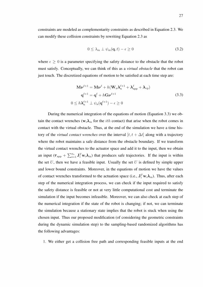
27

constraints are modeled as complementarity constraints as described in Equation 2.3. We

can modify these collision constraints by rewriting Equation 2.3 as

0 ≤ λin ⊥ ψin(q, t)− ε ≥ 0 (3.2)

where ε ≥ 0 is a parameter specifying the safety distance to the obstacle that the robot

must satisfy. Conceptually, we can think of this as a virtual obstacle that the robot can

just touch. The discretized equations of motion to be satisfied at each time step are:

Mν`+1 = Mν` + h(Wnλ`+1n + λ`

app + λvp)

q`+1 = q` + hGν`+1

0 ≤ hλ`+1n ⊥ ψn(q

`+1)− ε ≥ 0

(3.3)

During the numerical integration of the equations of motion (Equation 3.3) we ob-

tain the contact wrenches (wiλλλin for the ith contact) that arise when the robot comes in

contact with the virtual obstacle. Thus, at the end of the simulation we have a time his-

tory of the virtual contact wrenches over the interval [t, t + ∆t] along with a trajectory

where the robot maintains a safe distance from the obstacle boundary. If we transform

the virtual contact wrenches to the actuator space and add it to the input, then we obtain

an input (τττ app +∑nc

i=1 JTi wiλλλin) that produces safe trajectories. If the input is within

the set U , then we have a feasible input. Usually the set U is defined by simple upper

and lower bound constraints. Moreover, in the equations of motion we have the values

of contact wrenches transformed to the actuation space (i.e., JTi wiλλλin). Thus, after each

step of the numerical integration process, we can check if the input required to satisfy

the safety distance is feasible or not at very little computational cost and terminate the

simulation if the input becomes infeasible. Moreover, we can also check at each step of

the numerical integration if the state of the robot is changing; if not, we can terminate

the simulation because a stationary state implies that the robot is stuck when using the

chosen input. Thus our proposed modification (of considering the geometric constraints

during the dynamic simulation step) to the sampling-based randomized algorithms has

the following advantages:

1. We either get a collision free path and corresponding feasible inputs at the end

28

of the dynamic simulation step, or can terminate the simulation early if the input

required to obtain a collision free trajectory is infeasible. Moreover, we also get

the information of whether the robot gets stuck (i.e., its state does not change over

two consecutive iterations) for the chosen input and can terminate the simulation

after the robot reaches that state. At this state, any input in the conic hull of the

negative contact wrenches will not change the state of the robot. Thus, we can

easily check if a chosen input vector changes the state of the robot when it gets

stuck. Alternatively, we can easily find a vector that releases the robot from the

stuck state by checking if it lies in the conic hull formed by the contact wrenches.

2. When the input set of primitives is a finite set that is a subset of the feasible input

set obtained by discretization (say), there may be no input in the discretized set that

provides a collision free trajectory in the conventional algorithms. However, with

our algorithm, we may be able to obtain feasible inputs that lie outside the set of the

primitives. Thus, we may not be limited to the set of inputs that we start out with.

We note that in Equation 3.3, if we approximate the distance function ψn(q`+1) with a

Taylor’s series expansion, we will have a mixed linear complementarity system to be

solved at each step. The variables to be solved for at each step are ν`+1 and λ`+1n . Since

the mass matrix is positive definite, the matrix defining the LCP is positive definite. This

implies that there exists a unique solution to the LCP at each time step that can be ob-

tained in polynomial time (although for general LCPs the time taken for finding a solution

may be exponential in the number of variables).

3.4.1 Planning using a single potential field

In our algorithm, when we have an input that takes the robot directly towards the

goal, the robot may reach the goal even if the line joining the start and goal intersects

an obstacle. In other words, there are certain sets of obstacle arrangements and initial

and final configurations where we can obtain a feasible trajectory to the goal state with

a single attractive potential function with its minimum at the goal. This happens if the

obstacles are arranged such that the line joining the robot’s current state to the goal is

not normal to any of the obstacles it is intersecting with. For example, in Figure 3.1(b),

29

if the robot moves along the line joining S and G it will reach the goal. However, in

Figure 3.1(a), the robot will not reach the goal. Note that if the projection of the motion

of the robot in a time-step on the line joining the start and goal is always positive then the

robot always moves toward the goal. When the line joining the robot’s state and goal is

not normal to the surface of the obstacles it intersects, the above condition is true. Hence

the robot always reaches its goal. The input required to reach the goal is obtained from

the applied input plus the transformed contact wrenches.

3.4.2 Effect of choice of ∆t and input

As is evident from the discussion on sampling-based algorithms in Section 3.3 the

simulation time ∆t is a parameter to be chosen. Moreover, when the input set is given as

a compact set, the number of possible inputs is infinite. Thus, at each simulation step it

is not possible to check all possible inputs, and a subset of the available inputs is chosen

at each step. This subset may be randomly drawn or formed by discretizing the available

input set. To illustrate the effect of this let us consider a simple example as shown in

Figure 3.1(a). We consider a point particle that has to move from the start position S to

goal G. The particle can be independently actuated along the x and y axis (horizontal and

vertical directions in the figure). As can be seen from Figure 3.1(a), if we use the Newton-

Euler equations only for the dynamics, the planning algorithms will find a solution if and

only if the value of ∆t is chosen small enough and the input is small enough such that an

end state lies in the dashed triangular area. In contrast, the solution we will get from our

algorithm is shown by the bold line that is independent of the choice of ∆t. In our case

the choice of ∆t determines how fast the solution is found, but not whether the solution

can be found or not.

We also note that in our algorithm there is more flexibility to the choice of in-

puts. In the example in Figure 3.1(a), we will get a solution if our input set consists of

five primitive inputs, one input each along the positive and negative x−axis and y−axis

respectively and an input directly towards the goal. This is what we use in our implemen-

tations; two inputs along each of the independently actuated coordinates (one toward the

positive and one toward the negative axis) and an input directly towards the goal from the

current state. Using the inputs along the coordinates only is not enough, as can be seen

30

x

S

G

S

G

y

Figure 3.1: Schematic sketch of a situation where it is difficult to find a path usingmotions only along two directions.

in Figure 3.1(b). When the normal to the obstacle at the point of impact directly opposes

the input, the robot gets stuck.

3.4.3 Implication for narrow passage problems

The choice of the simulation time ∆t and the input set becomes critical in cluttered

environments because the probability of collision is very high. In such environments, it is

difficult to find a feasible input and it is well known that sampling-based algorithms for

kinodynamic planning perform poorly in such environments. Thus, in cluttered environ-

ments, i.e., environments characterized by the presence of narrow passages, our modifica-

tion would improve the performance of a sampling-based algorithm since it always finds a

collision free trajectory and the corresponding input. More specifically, if we arrive near

a narrow passage during the construction of the graph, then we are likely to find inputs

that will take us through the passage. Our algorithm does not say anything about how to

get near the narrow passage, which is very difficult to know.

3.4.4 Completeness Properties of our Algorithm

The change we are proposing to the existing sampling-based randomized planning

techniques enhances the reachability set at each point. In other words, for any varia-

tion of the randomized sampling-based techniques, the reachability set from any given

state, using our complementarity based dynamic simulation algorithm is a superset of

the reachability set using the conventional dynamic simulation. Thus all the probabilistic

completeness and resolution completeness results proved for any sampling-based algo-

rithm still holds with our variation.

31

3.4.5 Use of our algorithm for purely geometric problems

Although our algorithm is designed for problems where dynamics constraints need

to be considered, it may be useful even for motion planning problems with purely geo-

metric constraints. This is because in problems characterized by the existence of narrow

passages, it is difficult to get a sample in the narrow passages. However using a fake

dynamics for the robot and the complementarity constraints, we are guaranteed to get

samples in the free space, since all the configurations of the robot satisfying the comple-

mentarity constraints lie in the free space. Thus it may be easier to obtain samples in the

narrow passage once we are near the narrow passage.

3.5 Simulation ResultsIn this section we present some simulation examples illustrating our method. The

first example shows a scenario where a point robot reaches the goal under the action of a

single attractive potential field in the presence of obstacles. The obstacles hinder the mo-

tion along the direction of steepest descent of the potential function. The environment in

this case is not a star shaped environment and hence it is not possible to design navigation

functions that ensure that the goal can be reached. The second example is that of a 2R

planar manipulator moving among three obstacles. The problem is hand-designed so as

to contain two narrow passages in the free configuration space connected by a relatively

large free space region. The start and the goal configurations are placed at the two ends

of the narrow passage. In this case we use our modified version of the RRT algorithm to

obtain the solution trajectory.

3.5.1 Example 1: Planar point robot

This example illustrates planning with a single potential field at the goal in the

presence of obstacles. We consider a 2D point robot moving in a rectangular environment

with saw tooth shaped obstacles (see Figure 3.2). The saw tooth shaped obstacles form

a narrow passage in the environment and the start and goal configuration are located on

opposite sides of the obstacles. Let q = (x, y) be the configuration and ν = q be the

velocity of the robot. The discrete time dynamic model for state evolution of the system

32

0 1 2 3 4 5

−1.5

−1

−0.5

0

0.5

1

1.5

2

2.5

S G

Figure 3.2: Path of a point robot moving through a narrow passage formed by thewedge shaped obstacles

is

0 = −Mν`+1 + Mν` + Wnpn + papp

0 ≤ pn ⊥ ψn(q`) + WT

n ν`+1 ≥ ε(3.4)

where M is a 2× 2 diagonal matrix with the mass m of the robot as the diagonal entries,

Wn is a 2× 1 vector giving the normal at the contact point, ψn(q`) is the distance of the

robot to the obstacle at time `, and ε is the safety distance from the obstacle. Both the

distance and the normal at time ` are obtained from a collision detection algorithm. The

applied impulse is given by:

papp = −h(Kp(q` − qg) + Kdq

`) (3.5)

where Kp and Kd are diagonal matrices with positive entries, h is the time step, and

(q,ν) = (qg,0) is the goal state. The unknowns in Equation 3.4 are ν`+1 and pn. Thus,

we have a system of 3 equations and 3 unknowns.

33

3.2 3.4 3.6 3.8 4 4.2 4.4 4.6 4.8 5

−0.2

0

0.2

0.4

0.6

0.8

1

1.2

Figure 3.3: Enlarged portion of the path of the point robot that shows the safetydistance from the obstacle is maintained

For generating the results, we have used the following data: m = 1, ε = 0.01, α =

0.01, h = 0.01, each diagonal entry of Kp and Kd is 1, initial state is (0.4, 0.9, 0, 0) and

goal state is (5, 0.5, 0, 0). We simulated the system in Equation 3.4 using papp given by

Equation 3.5. The contact impulse obtained from the simulation Wnpn is then added

to the applied impulse to obtain the collision-free input impulse. The path taken by the

point robot to reach the goal under the action of the collision free input impulse is shown

in Figures 3.2 and 3.3. Note the approach of the robot to the goal state (when the x-

coordinate of the robot is greater than 4.5) that clearly shows the effect of dynamics. The

robot does not go straight to the goal because of its non-zero momentum in the direction

orthogonal to the goal direction. Ignoring the dynamics would give a solution path straight

to the goal (when there is no obstacle along the line joining the robot position to goal).

Figure 3.4 gives the velocities of the robot as it moves towards the goal. When the robot

reaches the safety distance from the wall the x-component of its velocity drops to 0 and

then becomes less than 0 as the y-momentum carries it along the obstacle. Near the end,

when there are no obstacles, the velocities decay to 0 because of the damping term in the

34

0 5 10 15 20 25 30 35 40−0.6

−0.4

−0.2

0

0.2

0.4

0.6

0.8

time (s)

Vel

ocity

(m

/s)

vx

vy

|v|

Figure 3.4: Velocity of the point robot

applied force. The top two subplots of Figures 3.5 and 3.6 show the x and y components

of the applied force and contact impulses obtained from the simulation step. The last

subplot in the figures show the x and y components of the collision-free input. The basic

RRT method could not find a solution to this problem with ∆t = 0.1 seconds and the

input set consisting of a random vector, a force towards the goal given by Equation 3.5,

and

u = {1

0

−1

0

0

1

0

−1

} (3.6)

3.5.2 Example 2: 2R Manipulator

The second example is that of a 2R manipulator (a planar manipulator with 2 revo-

lute joints, see Figure 3.7) that has to move from a start to goal configuration in a gravity

free environment with three circular obstacles (see Figure 3.13). The free space of the

manipulator relevant to the problem along with the start and goal configurations is shown

in Figure 3.8. Let the joint angles q = (q1, q2) be the configuration of the robot and ν = q

be the joint angle rates. The discrete time dynamic model for state evolution of the system

35

0 5 10 15 20 25 30 35 40−1

−0.5

0

0.5

1

1.5

Pot

entia

l For

ce (

N)

time (s)

0 5 10 15 20 25 30 35 40−0.4

−0.3

−0.2

−0.1

0

Con

tact

Impu

lse

(N−

s)

time (s)

0 5 10 15 20 25 30 35 40−0.3

−0.2

−0.1

0

0.1

Fin

al In

put I

mpu

lse

(N−

s)

time (s)

Figure 3.5: X-component of the forces/impulses acting on the point robot

is

0 = −Mν`+1 + Mν` − pvp + Wnpn + papp

0 ≤ pn ⊥ ψn(q`) + WT

n ν`+1 ≥ ε(3.7)

where the mass matrix and Coriolis force term are given by

M =

α + 2β cos(q2) δ + β cos(q2)

δ + β cos(q2) δ

pvp =

−β sin(q2)q

`2 −β sin(q2)(q

`1 + q`

2)

β sin(q2)q`1 0

q`

1

q`2

α = Iz1 + Iz2 + m1r21 + m2(l

21 + r2

1)

β = m2l1r2

δ = Iz2 + m2r22

(3.8)

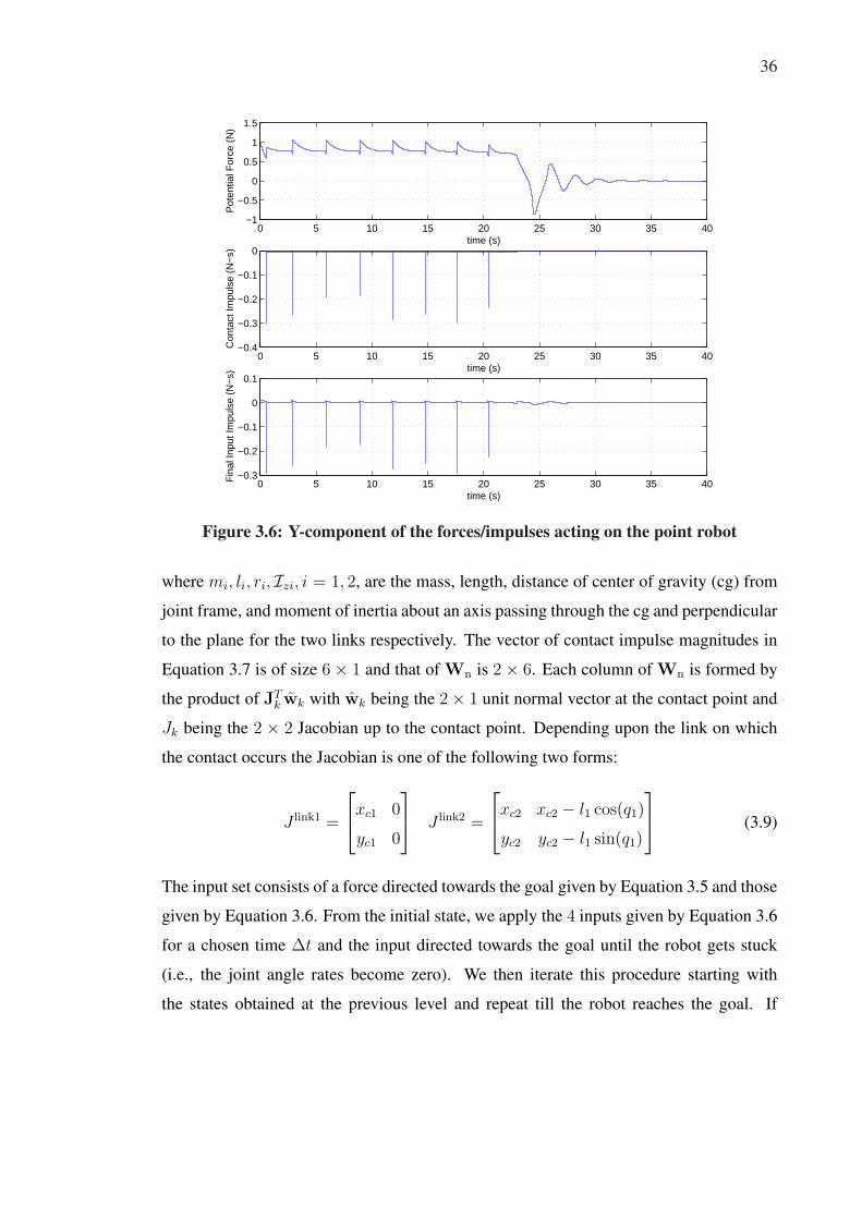
36

0 5 10 15 20 25 30 35 40−1

−0.5

0

0.5

1

1.5

Pot

entia

l For

ce (

N)

time (s)

0 5 10 15 20 25 30 35 40−0.4

−0.3

−0.2

−0.1

0

Con

tact

Impu

lse

(N−

s)

time (s)

0 5 10 15 20 25 30 35 40−0.3

−0.2

−0.1

0

0.1

Fin

al In

put I

mpu

lse

(N−

s)

time (s)

Figure 3.6: Y-component of the forces/impulses acting on the point robot

where mi, li, ri, Izi, i = 1, 2, are the mass, length, distance of center of gravity (cg) from

joint frame, and moment of inertia about an axis passing through the cg and perpendicular

to the plane for the two links respectively. The vector of contact impulse magnitudes in

Equation 3.7 is of size 6 × 1 and that of Wn is 2 × 6. Each column of Wn is formed by

the product of JTk wk with wk being the 2× 1 unit normal vector at the contact point and

Jk being the 2 × 2 Jacobian up to the contact point. Depending upon the link on which

the contact occurs the Jacobian is one of the following two forms:

J link1 =

xc1 0

yc1 0

J link2 =

xc2 xc2 − l1 cos(q1)

yc2 yc2 − l1 sin(q1)

(3.9)

The input set consists of a force directed towards the goal given by Equation 3.5 and those

given by Equation 3.6. From the initial state, we apply the 4 inputs given by Equation 3.6

for a chosen time ∆t and the input directed towards the goal until the robot gets stuck

(i.e., the joint angle rates become zero). We then iterate this procedure starting with

the states obtained at the previous level and repeat till the robot reaches the goal. If

37

r1

r2

q2

q1y

x

l1

l2

Figure 3.7: A planar manipulator with 2 revolute joints (2R manipulator).

the robot is at a stuck state and a particular input does not move it from that state, we

reject the input after two time-steps of dynamic simulation. Note that this is a very basic

version of RDT where we are growing the tree by expanding all the nodes. We obtain a

solution to our problem in three iterations. The number of nodes in the tree is 27. In our

simulations we have used the following data: m1 = m2 = 1, l1 = l2 = 1, r1 = r2 =

0.5, ∆t = 2s, h = 0.01s, initial state [0.22π, 1.94π, 0, 0], and goal state [0.5π, 0.1π, 0, 0].

The proportional and derivative gains, Kp and Kd, in Equation 3.5 are assumed to be 2×2

diagonal matrices. Each diagonal entry of Kp is 3 and Kd is 4. The basic RRT could not

find a solution to this problem with ∆t = 0.1 seconds.

Figure 3.8 shows the collision-free path of the robot in configuration space that we

obtained. Figure 3.9 shows the variation of joint angle rates in our solution as the manip-

ulator moves from start to goal state. Figures 3.10(a) and 3.11(a) show the input torques

at joint 1 and joint 2 respectively, during the search stage. The contact impulses projected

to the actuator space are shown in Figures 3.10(b) and 3.11(b). The final collision-free

input impulses at each joint that takes the manipulator from start to goal state are shown

in Figures 3.10(c) and 3.11(c). Figures 3.12, 3.13, and 3.14 show some snapshots of the

38

path of the manipulator in configuration space and work space. Note that Figures 3.12

and 3.8 are the same figure; the former is drawn at a lesser resolution so that the points in

the configuration space can be clearly identified visually.

q2 →

← q

1

S

G

Figure 3.8: Configuration space of the 2R manipulator. The white region shows thefree space. The path of the robot in the configuration space from startto goal is shown by the dotted line. The points S and G are the start andgoal configurations respectively.

3.6 ConclusionIn this chapter, we have shown the use of complementarity based dynamic simula-

tion algorithm in kinodynamic motion planning problems and pointed out its advantages

in solving certain narrow passage problems. We note that we have restricted our atten-

tion to problems without contact (or for problems involving collision avoidance only). In

principle our method also applies to applications where the robot may be in contact with

39

0 2 4 6 8 10 12 14−5

−4

−3

−2

−1

0

1

2

time (s)

Ang

ular

Vel

ocity

(ra

d/s)

Joint 1Joint2

Figure 3.9: Variation of the joint angle rates of the 2R robot for motion from startto goal configuration in Figure 3.8.

other objects. However, in problems involving contacts, the complementarity based sim-

ulations suffer from some drawbacks as depicted in Chapter 2. In the next two chapters

we present solutions that overcome these limitations.

40

0 5 10 15−2

0

2

4

App

lied

Tor

que

(N−

m)

(a)

0 5 10 15−1

0

1

2

Con

tact

Impu

lse

(N−

m−

s)

(b)

0 5 10 15−1

0

1

2

Fin

al In

put I

mpu

lse

(N−

m−

s)

time (s)

(c)

Figure 3.10: (a) The applied torque at joint 1 used for dynamic simulation (b) Thecontact impulses transformed to joint 1 obtained from dynamic simu-lation using the input in subplot (a). (c) The final collision free inputtorque impulse for joint 1.

41

0 5 10 15−4

−2

0

2

App

lied

Tor

que

(N−

m)

(a)

0 5 10 150

0.2

0.4

0.6

0.8

Con

tact

Impu

lse

(N−

m−

s)

(b)

0 5 10 15−0.2

0

0.2

0.4

0.6

Fin

al In

put I

mpu

lse

(N−

m−

s)

time (s)

(c)

Figure 3.11: (a) The applied torque at joint 2 used for dynamic simulation (b) Thecontact impulses transformed to joint 2 obtained from dynamic simu-lation using the input in subplot (a). (c) The final collision free inputtorque impulse for joint 2.

42

q2

q 1

S

1

G 2

3

4

5

6 7

8

Figure 3.12: Configuration space of the 2R manipulator. The white region shows thefree space. The black squares show configurations along the collision-free trajectory. The positions of the manipulator in the workspace cor-responding to the configurations are shown in Figures 3.13 and 3.14.The points S and G are the start and goal configurations respectively.

43

−1 −0.5 0 0.5 1 1.5

−0.2

0

0.2

0.4

0.6

0.8

1

1.2

1.4

1.6

1.8

S

G

1

2

3 4

Figure 3.13: The first four configurations in the path of the 2R robot for motion fromstart to goal configuration in Figure 3.12.

−1 −0.5 0 0.5 1 1.5

−0.2

0

0.2

0.4

0.6

0.8

1

1.2

1.4

1.6

1.8

S

G

5

6

7

8

Figure 3.14: The last four configurations in the path of the 2R robot for motion fromstart to goal configuration in Figure 3.12.

CHAPTER 4Proximity Queries between Convex Objects

4.1 IntroductionIn this chapter we study the problem of computing the closest points on two convex

objects, when each object is described as an intersection of implicit surfaces. Distance

computation algorithms are usually used in the narrow phase of a collision detection al-

gorithm in applications where knowledge of the closest points is required rather than

just a yes/no answer for collision. Such applications are characterized by existence of

intermittent contact, i.e., phases of contact and no contact between the objects, with a

concomitant need to predict potential contact points. Some example applications are dy-

namic simulation [3, 77, 106], dexterous manipulation [79, 10], computer animation [14],

and haptics [73, 25]. Other applications where collision avoidance is the primary goal

may also make use of the knowledge of the closest distance information. Examples of

such applications include robot path planning [90] and spacecraft safe volume computa-

tions [26].

It is well known that the evolution of contact points for continuous contact states

depends on the relative curvature of the two contacting bodies [78, 62]. Polygonalization

may lead to poor approximation of the object curvature and consequently affect the ac-

curacy of the dynamic simulation. For applications in motion planning and engineering

analysis of objects in intermittent contact [104], such discretization may not be desirable

(see rolling disc example in Chapter 2). More generally, polygonalized representations

of smooth objects can lead to intermittent loss of contact and bouncing in the simula-

tions. The effect of shape and surface curvature on the dynamic motion of contacting

objects is dramatically illustrated by a spinning boiled egg and toys such as the rattleback

(or Celtic wobblestone) [97, 40]. Similarly, exact representation of shape is important

when modeling robot fingers in contact with smooth objects during multi-finger dexter-

ous manipulation (Figure 4.1). Determining the first contact point correctly when fingers

reposition during finger gaiting is useful since the manipulation operations are sensitive

to the contact point and the normal and curvature at that point [10, 85].

44

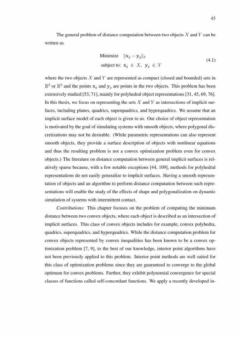
45

The general problem of distance computation between two objects X and Y can be

written as

Minimize ‖xg − yg‖2

subject to: xg ∈ X, yg ∈ Y(4.1)

where the two objects X and Y are represented as compact (closed and bounded) sets in

R2 or R3 and the points xg and yg are points in the two objects. This problem has been

extensively studied [53, 71], mainly for polyhedral object representations [31, 45, 69, 76].

In this thesis, we focus on representing the sets X and Y as intersections of implicit sur-

faces, including planes, quadrics, superquadrics, and hyperquadrics. We assume that an

implicit surface model of each object is given to us. Our choice of object representation

is motivated by the goal of simulating systems with smooth objects, where polygonal dis-

cretizations may not be desirable. (While parametric representations can also represent

smooth objects, they provide a surface description of objects with nonlinear equations

and thus the resulting problem is not a convex optimization problem even for convex

objects.) The literature on distance computation between general implicit surfaces is rel-

atively sparse because, with a few notable exceptions [44, 109], methods for polyhedral

representations do not easily generalize to implicit surfaces. Having a smooth represen-

tation of objects and an algorithm to perform distance computation between such repre-

sentations will enable the study of the effects of shape and polygonalization on dynamic

simulation of systems with intermittent contact.

Contributions: This chapter focuses on the problem of computing the minimum

distance between two convex objects, where each object is described as an intersection of

implicit surfaces. This class of convex objects includes for example, convex polyhedra,

quadrics, superquadrics, and hyperquadrics. While the distance computation problem for

convex objects represented by convex inequalities has been known to be a convex op-

timization problem [7, 9], to the best of our knowledge, interior point algorithms have

not been previously applied to this problem. Interior point methods are well suited for

this class of optimization problems since they are guaranteed to converge to the global

optimum for convex problems. Further, they exhibit polynomial convergence for special

classes of functions called self-concordant functions. We apply a recently developed in-

46

Figure 4.1: A dexterous manipulation task that requires closest distance computa-tions to predict the contact points of fingers with an object. The fingersand object are represented as superquadrics.

terior point algorithm [11, 116] to compute the distance between convex implicit surface

objects and demonstrate that it is particularly effective for this class of problems. For

polyhedral and quadric surfaces, the algorithm takes O(n1.5) time, where n is the num-

ber of constraints. We also illustrate the approach on surfaces such as superquadrics and

hyperquadrics. To the best of our knowledge, this is the first approach with this demon-

strated capability (without discretization). Another important advantage of this method

is that it provides a uniform framework for proximity queries between objects described

as intersections of convex polyhedra, quadrics, or any arbitrary convex implicit surface.

Further, these proximity queries can be used in the narrow phase of hierarchical collision

detection for implicit surfaces. We present implementation results for example implicit

surface objects that show that the algorithm exhibits linear time performance in practice,

and demonstrate that distance computation rates of about 1 kHz can be achieved. We also

extend the approach to proximity queries between deforming convex objects. Finally, we

show that continuous collision detection for linearly translating objects can be performed

by solving two related convex optimization problems. For polyhedra and quadrics, we es-

tablish that the time complexity of this continuous collision detection problem is O(n1.5).

The chapter is organized as follows. After a discussion of related work in Sec-

47

tion 4.2, we review the mathematical background for our work in Section 4.3. We present

the formulation of the closest distance problem in Section 4.4 and describe how it can be

solved using interior point algorithms in Section 4.5. Section 4.6 provides theoretical and

practical results on the complexity of the closest point algorithm. Section 4.7 extends the

approach to continuous proximity queries for linearly translating objects. We present our

implementation results in Section 4.8 and conclude with a discussion of future work in

Section 4.9. The work in this chapter has appeared in [21, 22].

4.2 Related WorkProximity queries for polyhedra: Proximity queries and collision detection algo-

rithms have an extensive literature in computational geometry [31], robotics [45, 69],

and computer graphics [109]. We provide a sampling of the related work in these areas;

see [71, 53] for an overview of collision detection and proximity queries. When colli-

sion detection algorithms estimate the distance between two objects, they typically use

a geometric approach. Popular algorithms for convex polyhedra include GJK [45], Lin-

Canny [69], and V-Clip [76]. GJK [45] is an iterative algorithm for distance computation

between two convex polyhedra. It uses a support function description of the polyhedra

and takes time linear in the number of vertices. Lin-Canny [69] efficiently computes

the distance between two convex polyhedra and tracks the closest points using adjacency

of features. Its running time is linear in the number of features (faces, edges, and ver-

tices). Both algorithms can track the closest points in (almost) constant time when there

is temporal coherence [13]. Bobrow [7] proposed an optimization based approach for

computing the distance between two convex polyhedra. He formulated the problem as

a quadratic programming problem and used a gradient projection algorithm to solve the

problem. However this approach can suffer from convergence issues [122].

Proximity queries for quadrics and NURBS: Distance estimation between non-

polyhedral shapes has focused primarily on quadrics and NURBS surfaces. Among the

algorithms for polyhedra, only GJK has been extended directly for smooth convex ob-

jects [44]; van den Bergen [109] discusses in detail a GJK implementation for convex

quadric objects. However this GJK algorithm does not guarantee convergence in a finite

number of steps. Further, computing the support mapping is difficult for superquadrics

48

with fractional (non-integer) exponents due to the difficulty of solving polynomial equa-

tions with fractional exponents. Turnbull and Cameron [28] extended GJK to convex

NURBS surfaces. They describe a procedure to calculate the support mapping for the

NURBS surfaces which reduces to solving two nonlinear polynomial equations in two

parameters. They present results for 2D and describe the theory for 3D. Baraff [3] de-

scribed collision detection algorithms for implicit and parametric curved convex surfaces.

He uses the collinearity property of the surface normals of the closest points to numeri-

cally compute closest points at the initial configuration. He exploits geometric coherence

to compute closest points at subsequent configurations. Lin and Manocha [70] consider

curved models described as NURBS surfaces and piecewise algebraic surfaces. Using the

collinearity property of the surface normals, they describe the closest points using a set

of polynomial equations. However, the number of roots can be prohibitively large as it

depends on the degree of the polynomials describing the surfaces; the roots must be ex-

amined to identify the closest points. Note also that it is not possible to obtain bounds on

the number of roots for systems of equations with fractional indices (as would arise with

superquadrics). Schomer et al. [98] describe a collision detection algorithm for curved

objects bounded by quadric surface patches by finding roots of univariate polynomials

of degrees 4 and 8. Johnson and Cohen [54] give a lower-upper bound tree framework

for distance computation between any two object representations for which the follow-

ing set of operations is available: bounding volume generation, lower and upper bound

on distance, bounding volume refinement, and determination of computation termination.

They have demonstrated their method on polyhedra as well as NURBS surfaces. Patoglu

and Gillespie [83] perform real-time tracking of the closest points between two objects

modeled with parametric surfaces by formulating it as a control problem and exploiting

spatial and temporal coherence.

The literature on distance computation between general implicit surfaces is rela-

tively sparse because, with the exception of GJK, methods for polyhedral representations

do not easily generalize to implicit surfaces. In fact, no closed form solution exists even

for the distance between a point and an ellipsoid. Most closely related is recent work

on computing the distance between two ellipsoids and other conic sections [68, 26, 100].

Sohn et. al. [100] exploit the fact that the closest points on two surfaces are where their

49

common normals intersect the surfaces. They apply their line geometry approach to el-

lipsoids, for which the minimum distance computation is reduced to finding the common

roots of two polynomial equations of degree 8 and 16. Coppola and Woodburn [26] for-

mulate the problem as an optimization problem. They iteratively solve the problem of

closest distance from a point to an ellipsoid to arrive at the optimal solution. Rimon and

Boyd [92] use convex optimization techniques to find the minimum volume enclosing

ellipsoids to model objects, and then compute a conservative distance estimate between

ellipsoids by treating it as an eigenvalue problem. Choi et al. [23] present a continuous

collision detection algorithm for two elliptical disks moving in the plane. Collisions are

identified by checking for the real roots of the univariate discriminant of the character-

istic equation of the two moving ellipses. Although superquadrics are a generalization

of quadrics, the problem in generalizing the methods in [3, 45, 26, 100] to superquadrics

is that they all lead to polynomial equations with fractional exponents, which are very

difficult to solve. In general, we do not know the total number of roots, and even when it

is possible to simplify the polynomials, they may have large integer exponents.

4.3 Mathematical PreliminariesWe now review the mathematical terminology that will be used in the rest of the

chapter.

Convex Set: A set U ⊆ Rn is called a convex set if for any two points u1, u2 ∈ U and any

λ with 0 ≤ λ ≤ 1, we have

λu1 + (1− λ)u2 ∈ U.

Convex Function: A function f : Rn → R is convex if the domain of f (dom f ) is a

convex set and for all u1, u2 ∈ dom f and any λ with 0 ≤ λ ≤ 1, we have

f(λu1 + (1− λ)u2) ≤ λf(u1) + (1− λ)f(u2).

50

Convex Programming Problem: Consider the general nonlinear programming problem

given by:

Minimize f0(x)

subject to: x ∈ U(4.2)

This nonlinear programming problem is called a convex programming problem if the

objective function f0 is a convex function and the feasible set U is a convex set [5].

Usually the set U is defined by a set of inequality and/or equality constraints. If the

inequality constraints defining U are convex functions and the equality constraints are

linear, then U is a convex set [9].

Superquadric: A superquadric [49] is defined by the equation

f(x) =

∣∣∣∣x1

a1

∣∣∣∣n1

+

∣∣∣∣x2

a2

∣∣∣∣n2

+

∣∣∣∣x3

a3

∣∣∣∣n3

− 1 = 0

ni = li/mi, li,mi ∈ Z+, i ∈ {1, 2, 3}f(x) convex if 1 ≤ ni < ∞f(x) nonconvex if 0 < ni < 1

(4.3)

Although the definition here differs slightly from that in [4], the two definitions are equiv-

alent [49]. Convex superquadrics are a broad class of shapes that include cuboids, rounded

cuboids, ellipsoids, spheres, and (rounded) octahedra. The planes∣∣∣xi

ai

∣∣∣ ≤ 1, i = 1, 2, 3

define a bounding cube for the superquadric and the indices control the roundedness of

the shape. Different shapes can be obtained by varying ni. The shape is a rhomboid when

ni = 1, and the shape becomes a cube as ni tends to infinity.

51

Hyperquadric: A hyperquadric [49] is defined by the equation

f(x) =N∑

i=1

|Hi(x)|ni − 1 = 0 where N ≥ 3 and

Hi(x) = (aix1 + bix2 + cix3 + di)

ni = li/mi, li,mi ∈ Z+

f(x) convex if 1 ≤ ni < ∞f(x) nonconvex if 0 < ni < 1

(4.4)

Hyperquadrics are a more general class of shapes than superquadrics. In particular, they

include asymmetric shapes. In this case also, the intersection of the planes Hi(x) ≤ 1

form a bounding polytope for the hyperquadric and the indices control the roundedness

of the shape.

Self-concordant functions: A convex function f : R → R is self-concordant if

|f ′′′(x)| ≤ 2f ′′(x)3/2 for all x ∈ domf .

A convex function f : Rn → R is self-concordant if it is self-concordant along every line

in its domain (see [9] for details).

4.4 Problem FormulationIn this section we present the formulation of the minimum distance computation

problem. We first outline a geometric approach to the minimum distance problem that

has been popular in prior work on non-polyhedral objects [3, 70, 100] and connect it to

an optimization formulation. Let fX be an implicit function representing object X and

fY be an implicit function representing object Y , and let xg, yg be the global coordinates

of points in X and Y respectively. To compute the closest distance between X and Y , the

approach uses the geometric condition that the normals on the two surfaces at the closest

points are aligned with each other. Using this and the condition that the closest points

should lie on the surfaces of the two objects, we can obtain the closest points by solving

52

the following system of nonlinear equations

xg − yg = −λX∇fX(xg)

xg − yg = λY∇fY (yg)

fX(xg) = 0

fY (yg) = 0

(4.5)

where λX and λY are scalars. The conditions given by Equation 4.5 are precisely the

Karush-Kuhn-Tucker (KKT) conditions for solving the following optimization problem.


subject to: fX(xg) = 0

fY (yg) = 0

(4.6)

However note that when fX and fY are nonlinear, the above problem is nonconvex even

when the objects are convex and the solution can therefore get stuck in a local minimum.

We now formulate the problem of minimum distance computation between two

convex objects as a convex optimization problem. Each object is assumed to be described

as an intersection of a finite number of implicit primitives (i.e., a finite number of algebraic

inequalities). In general, each of the intersecting surfaces may be specified in its own

reference frame. The distance computation problem of Equation 4.1 can then be written

as


subject to: xg = Rxixli + pxi i = 1, . . . , m

yg = Ryjylj + pyj j = m + 1, . . . , n

fi(xli) ≤ 0 i = 1, . . . , m

fj(ylj) ≤ 0 j = m + 1, . . . , n

(4.7)

where xg, yg ∈ R3 are the global coordinates of points in the two objects X and Y

respectively; Rki,pki, k = x, y, are the rotation matrix and position of the reference

frame of each of the intersecting surfaces with respect to the global frame, xli, ylj ∈ R3

53

are the coordinates of the points in the local reference frames of the surfaces, and fk (k =

i, j) are the functions representing the implicit surfaces in the local reference frames. The

above system has 3n linear equality constraints and n inequality constraints. Note that the

linear constraints in Equation 4.7 can be any affine transformation (not necessarily a rigid

body transformation). In particular, we can handle global deformations like nonuniform

scaling by post multiplying the rotation matrix with a scaling matrix.

From the linear constraints in Equation 4.7 we can easily evaluate xli and ylj and so

the inequality constraints can be expressed in terms of xg and yg. Therefore, without loss

of generality, we can assume that the implicit surface describing the objects is described

in a global reference frame. The distance computation problem of Equation 4.1 is then

given by


subject to: fi(xg) ≤ 0 i = 1, . . . , m

fj(yg) ≤ 0 j = m + 1, . . . , n

(4.8)

where fk (k = i, j) are the functions representing the implicit surfaces in the global ref-

erence frame. The above system has n inequality constraints. The objective function

in Equation 4.8 is convex, and if the inequalities represent a convex set (i.e., the ob-

jects are convex), the minimum distance computation problem is a convex programming

problem. For general convex surfaces, the distance computation problem is a nonlinear

program (NLP). For objects described as convex quadric surfaces, the problem reduces

to a quadratically constrained quadratic program (QCQP), and if the objects are convex

polyhedra (intersections of planes), the closest distance problem becomes a quadratic

programming (QP) problem.

The solution to the minimum distance problem of Equation 4.8 gives two closest

points that lie on the surfaces of the two objects (i.e., boundaries of the two sets). We use

an interior point algorithm [11] for solving this problem. See Figure 4.2 for an example

solution generated using an interior point algorithm. Interior point methods [118] are

a class of optimization algorithms for nonlinear programming problems. In contrast to

algorithms for finding the closest points that generate iterates that lie on the surface of

the objects (gradient projection [7], for example), feasible interior point methods generate

54

02

4 0 1 2 3 4

−1

0

1

2

3

4

5

6

yx

z

III

II

I

Figure 4.2: Three example objects. The closest points of each pair of objects areshown connected by a line segment.

iterates that are guaranteed to lie inside the objects and converge towards the closest points

on the boundaries of the objects. This is the main conceptual difference between interior

point methods and other methods. Sequential quadratic programming (SQP) is another

method for solving general nonlinear programming problems [46]. In contrast to SQP,

interior point methods have polynomial time convergence guarantees for certain convex

problems, as we describe in Section 4.6. Moreover, an informal comparison of SQP

implementations with interior point algorithm implementations on the NEOS server [29]

shows the interior point methods to be slightly faster. Therefore, we choose to solve the

optimization problem with an interior point algorithm.

4.5 Interior Point AlgorithmIn this section, we present the primal-dual interior point algorithm for solving the

optimization problem described in Equation 4.8. The Karush-Kuhn-Tucker (KKT) condi-

tions give necessary and sufficient conditions for solving the minimum distance problem

in Equation 4.8, since it is a convex optimization problem and satisfies Slater constraint

qualification. For ease of presentation, we rewrite Equation 4.8 in a general nonlinear

55

program format as

Minimize f0(x)

subject to: f(x) + s = 0

s ≥ 0

(4.9)

where f0(x) = ‖xg −yg‖22, x = [xT

g ,yTg ]T is a 6× 1 column vector, s is an n× 1 column

vector of slack variables, and f : R6 → Rn is the vector of inequality constraints. The

Lagrangian for the above constrained optimization problem can be written as

f0(x) + λT(f(x) + s) (4.10)

where λ is an n×1 vector of Lagrange multipliers. The KKT conditions for Equation 4.9

are the system of nonlinear equations below:

∇f0(x) + (∇f(x))T λ = 0

f(x) + s = 0

LSe = 0

(4.11)

Here L is an n×n diagonal matrix of the λ variables, S is an n×n diagonal matrix of the

slack variables s, and e is an n-vector of ones. The above is a system of 2n + 6 nonlinear

equations in the 2n + 6 variables x, λ, s. Equation 4.11 can be solved by Newton’s

method for solving systems of nonlinear equations. It converges to the correct solution

if the initial guess is near enough [80]. However, in general, it is very difficult to supply

a good initial guess and there is then no guarantee that Newton’s method will converge.

The main difficulty in using Newton’s method is that we have to ensure s≥ 0, which may

lead to very small step lengths that result in convergence problems.

Interior point methods are a general class of algorithms for solving nonlinear pro-

gramming problems. In essence, these methods approximately solve a sequence of sys-

tems of nonlinear equations that are formed by perturbing the complementarity equations

(LSe = 0) in the KKT conditions. Following [9], we present the interior point method by

56

reformulating Equation 4.9 as a barrier problem.

Minimize f0(x)− µ

n∑i=1

ln(si)

subject to: f(x) + s = 0

(4.12)

The formulation in Equation 4.12 is the barrier formulation [9] of the minimum distance

problem of Equation 4.9 and µ is called the barrier parameter, with µ > 0. Equation 4.12

differs from Equation 4.9 in that the non negativity constraints on s are not present ex-

plicitly, but are implicit in the objective. The Lagrangian for the above constrained opti-

mization problem can be written as

f0(x)− µ

n∑i=1

ln(si) + λT(f(x) + s) (4.13)

where λ is the vector of Lagrange multipliers. Thus, the KKT conditions can be written

as

∇f0(x) + (∇f(x))T λ = 0

f(x) + s = 0

LSe− µe = 0

(4.14)

The above equation represents a system of 2n+6 nonlinear equations in 2n+6 variables

and can be approximately solved for a given µ. Note that Equation 4.11 and Equation 4.14

differ in the complementarity conditions. As the barrier parameter µ approaches 0, the

KKT conditions for the barrier problem (Equation 4.14) approach the KKT conditions of

the original problem (Equation 4.11). See Figure 4.3 for a schematic illustration of the

interior point method.

For our proximity query problem, feasible interior point methods generate iterates that

yield points guaranteed to lie inside the objects and converge towards the closest points

on the boundaries of the objects. See the example proximity query in Figure 4.4.

The general structure of interior point methods is indicated in Algorithm 2, where

termination criterion 1 is the ending condition for the whole problem (Equation 4.11) and

termination criterion 2 is the ending condition for approximately solving Equation 4.14

57

Central Path

Figure 4.3: Schematic illustration of the interior point method for a path followingalgorithm. The convex region represents the feasible set. The centralpath is an arc of strictly feasible points that solve Equation 4.14 as theparameter µ approaches 0. The progress of the iterates generated by theinterior point solver is indicated by the polygonal line connecting them.The iterates are guaranteed to lie within a neighborhood, represented bythe circular ball, of the central path.

for the current value of µ. The outer while loop determines the number of times µ has to

be updated, i.e., the number of times Equation 4.14 has to be approximately solved for

the sequence of µ values. The inner while loop is a variant of Newton’s method used for

approximately solving Equation 4.14 for a fixed value of µ. The different interior point

implementations (KNITRO [11, 116], LOQO [111], IPOPT [115]) vary in the way they

calculate the step lengths for a particular value of µ, the termination criteria they use, and

the way in which they update µ.

4.6 Computational ComplexityThe total cost of solving a problem using Algorithm 2 is the product of the total

number of iterations (considering both loops) and the computational effort in solving

the system of linear equations to determine the Newton direction in each iteration. The

system of linear equations to be solved to determine the Newton direction is

A1 A2T 06×n

A2 0n×n In×n

06×n S L

∆x

∆λ

∆s

=

−F1

−F2

−F3

(4.15)

58

−1 0 1 2 3 4−1

−0.5

0

0.5

1

1.5

2

2.5

3

3.5

4Progress of the Iterates in Interior point method

x

y

Figure 4.4: Example illustrating the sequence of closest point estimates generated bythe interior point method for two 2D superquadric objects, with indices(23

11, 11

5), (76

7, 71

5) and semiaxes 1. The iterates of the interior point method

are mapped to corresponding points in the objects.

where A1 = ∇2f0(x) +∑n

i=1λi∇2fi(x) is a 6×6 matrix, A2 =∇f(x) is a n×6 matrix,

the definitions of S and L are the same as before, and F1 = ∇f0(x) + (∇f(x))T λ,

F2 = f(x) + s, F3 = LSe− µe.

In general, the computational cost of solving a system of n linear equations in n

unknowns is O(n3). However, we now establish that the system of linear equations can

be solved in O(n) time. By simple algebraic manipulation of the above equations, we

obtain the following formulas for ∆x, ∆λ, and ∆s:

∆x = G−1(−F1 −AT2 (S−1L)(F2 + L−1F3))

∆λ = (S−1L)(A2∆x− F2 + L−1F3)

∆s = −L−1(F3 + S∆λ)

(4.16)

where G = A1 + AT2 (S−1L)A2. Since G is a 6 × 6 matrix, G−1 can be computed in

constant time. Moreover, S and L are n × n diagonal matrices, so S−1 and L−1 can be

computed in linear time. Thus we can compute all the inverses in O(n). Moreover, noting

the dimensions of A1 and A2, we can see by inspection that the matrix multiplication also

requires O(n) operations. So Equation 4.16 can be evaluated in O(n) time, or in other

59

Algorithm 2 Interior point algorithmInput: initial strictly feasible x0, initial barrier parameter µ0, specified tolerance ε,and KKT equationsOutput: Closest points solution x

k ← 0while termination criterion 1 not satisfied do

while termination criterion 2 not satisfied doSolve the system of linear equations // determine Newton directionDetermine step length αk by line searchxk+1 ← xk + αk∆xk

sk+1 ← sk + αk∆sk

λk+1 ← λk + αk∆λk

k ← k + 1end whileµ← cµ // c < 1, may be constant or adaptive

end whilereturn xk

words, the computation of the Newton step takes O(n) time. Note that we have not made

any assumptions regarding the primitive surface describing the object. Thus this analysis

is valid for any implicit surface (including planes, quadrics, superquadrics, hyperquadrics,

etc.) and for intersections of these implicit surfaces.

For general functions, there is no known bound on the total number of iterations

(including both while loops). However, if the log barrier function of the implicit surface

constraints is a self-concordant function (refer to Section 4.3), the number of Newton

iterations (which is the number of times Equation 4.15 must be solved) is polynomial

in a parameter depending on the structure of the function. For polyhedral constraints

and quadric constraints the number of Newton iterations required for converging to the

optimal solution is O(n0.5). This implies that the theoretical complexity of our approach

for polyhedra and quadrics is O(n1.5). Although algorithms with theoretical linear time

guarantees are available for polyhedra, for the case of quadrics, as far as we know, this is

the best known bound. Moreover, our experiments indicate the algorithm exhibits linear

time behavior in practice, as shown in Figure 4.5 and Figure 4.6.

For superquadrics and hyperquadrics, the log barrier function might not be self-

concordant in the general case. However, note that superquadric and hyperquadric func-

tions have self-concordant barriers because they define convex regions, and every convex

60

0 2000 4000 6000 8000 10000−500

0

500

1000

1500

2000

Number of Planes

Run

ning

Tim

e (m

illis

econ

ds)

Figure 4.5: Plot showing observed linear time behavior of the interior point algo-rithm for polyhedra.

10 20 30 40 50 60 70 80 90 1000

1

2

3

4

5

6

7

8

9

Number of Quadric Constraints

Run

ning

Tim

e (m

illis

econ

ds)

Figure 4.6: Plot showing observed linear time behavior of the interior point algo-rithm for quadrics.

region has a self-concordant barrier (its universal barrier). If this barrier is too hard to

find to be useful computationally, an alternative is to decompose the function into sim-

pler functions (for example, as second order cones [86]) such that the sum of the barriers

for the simpler functions gives a barrier for the original superquadric or hyperquadric.

However these representations may lead to computationally slower solutions due to the

increased number of variables and constraints. Glineur and Terlaky [47] provide self-

concordant formulations for lp-norm minimization that apply to superquadrics and hyper-

61

10 20 30 40 50 60 70 80 90 1000

2

4

6

8

10

12

14

Number of Superquadric Constraints

Run

ning

Tim

e (m

illis

econ

ds)

Figure 4.7: Plot showing observed linear time behavior of the interior point algo-rithm for superquadrics.

quadrics. However the computational performance of these formulations has not yet been

explored in the literature. Moreover, the observed time complexity of the interior point

algorithm is linear for this class of shapes (Figure 4.7), which implies that in practice the

number of iterations is constant, i.e., independent of the size of the problem. The ob-

served linear time behavior of the interior point algorithm even without self-concordant

representations further justifies the use of an interior point-based solver for this generic

nonlinear programming formulation.

4.7 Continuous Proximity Queries for Translating ObjectsWe now address the problem of continuous proximity queries for two linearly trans-

lating objects. Such queries can be useful in identifying feasible object motions during

assembly planning. The goal is to determine the exact time at which the two moving

objects are closest, without discrete sampling of their configurations. This computation

of the closest distance between two swept objects is closely related to the problem of

continuous collision detection ([15], [12], [120], [95], [91], [110]), where the time of first

contact between two colliding objects is to be determined; however most prior work has

been restricted to polyhedral objects. The advantage of such continuous collision detec-

tion methods is the ability to detect collisions even for fast moving objects in the presence

of thin obstacles.

62

We address the continuous collision detection problem for linearly translating ob-

jects by solving two related convex optimization problems. Assume the objects are mov-

ing along piecewise linear paths. Let X and Y be two objects described by fX(xl) ≤ 0

and fY (yl) ≤ 0. Let the two objects be linearly translating along the directions specified

by the unit vectors gx and gy with constant velocities vx and vy respectively. The fol-

lowing optimization problem finds the minimum distance between the two objects in the

time interval [0, tmax], where each object is moving along a single line segment. If the

minimum distance is greater than zero, the solution provides the closest points and the

time t at which the objects are closest. See Figure 4.8.


subject to: xg = Rxxl + px + vxtgx

yg = Ryyl + py + vytgy

fX(xl) ≤ 0

fY (yl) ≤ 0

t ≤ tmax

t ≥ 0

(4.17)

When the objects intersect, the problem above has multiple solutions corresponding

to zero distance. The time of first contact can be obtained by solving another convex

optimization problem using the solution of Equation 4.17. Let Q be the set of intersecting

points and q ∈ Q be a point specified in the global coordinate system. To obtain the time

of first contact, we solve the problem below, starting from an initial feasible guess that is

the solution of Equation 4.17.

63

−4 −3 −2 −1 0 1 2 3 4 5 −20

2−2

−1

0

1

2

3

4

5

6

yx

z

Figure 4.8: Computing the instant of closest distance using the continuous proximityquery. The bold blue line connects the closest points on the two objects,as they translate along the indicated line segments.

Minimize t

subject to: q = Rxxl + px + vxtgx

q = Ryyl + py + vytgy

fX(xl) ≤ 0

fY (yl) ≤ 0

tp ≥ t ≥ 0

(4.18)

where tp is the time obtained from the solution of Equation 4.17. See the example in

Figure 4.9.

We now establish that the computational complexity of solving the Newton step in

the continuous collision detection problem along a single linear segment is O(n), which is

the same as for the static query problem. We can eliminate xl and yl from Equation 4.17

and can write it in the form of Equation 4.9 where x is a 7×1 column vector that includes

t. Thus in Equation 4.15, A1 is a 7 × 7 matrix and A2 is an n × 7 matrix. This implies

that G is still a constant sized 7 × 7 matrix and the complexity argument for solving

Equation 4.16 in Section 4.6 applies directly. Similarly in Equation 4.18, x is a 4 × 1

vector consisting of q and t. Thus A1 is a 4 × 4 matrix and A2 is an n × 4 matrix and

64

−4 −3 −2 −1 0 1 2 3 4 5−2

0

2

−2

−1

0

1

2

3

4

5

y

x

z

Figure 4.9: Computing the time of first contact using the continuous proximityquery gives the solution to the continuous collision detection problem.

G is a 4 × 4 matrix. Hence the computation of the Newton step in both problems takes

O(n) time irrespective of the implicit primitive. Moreover, as the constraints have a self-

concordant log barrier function for the case of planes and quadrics, the overall complexity

is O(n1.5) in these cases.

Obtaining the collision interval for motion with known linear paths: Computing the

path intervals over which two robots can collide is useful in multiple robot coordination

problems where the robots travel along known paths [86]. When we are given the paths

traversed by the objects and wish to determine the path intervals over which the objects

could collide with each other, we solve the following optimization problem.

Minimize sx

subject to: xg = Rxxl + px + sxgx

yg = Ryyl + py + sygy

fX(xl) ≤ 0

fY (yl) ≤ 0

fX(yg) ≤ 0

fY (xg) ≤ 0

sx, sy ≥ 0

(4.19)

65

Here sx and sy represent the path lengths traversed by the objects. The inequalities

fX(yg) ≤ 0 and fY (xg) ≤ 0 describe all points in the intersection of both objects, and

also encode the constraint that the distance between the objects is zero. In fact, we have to

solve three more variations of the above problem with the objective function minimizing

−sx, sy, and −sy to find the minimum and maximum values of sx and sy. These define

corresponding collision intervals over the path for each object.

4.8 Results

I II III

IV V VI

Figure 4.10: Example objects. Objects I–III are superquadrics, IV is an intersectionof superquadrics and halfspaces, and V–VI are hyperquadrics.

We now present results illustrating our approach. To solve the distance computation

problem, we used KNITRO 5.0, a commercially available interior point based solver ([11,

116]). We use the primal-dual feasible interior point method in KNITRO, where all the

iterates are feasible. We have an initial feasible solution trivially from points at the centers

of the objects. The barrier parameter µ is initially set to 0.1 and reduced by an adaptive

factor at each iteration based on the complementarity gap. For each value of µ the system

66

of nonlinear equations is approximately solved by Newton’s method with the step size

determined by a trust region method [80].

We depict six example objects in Figure 4.10, three of which are superquadrics. The

indices and semiaxes of the three superquadrics are (43, 7

5, 15

13) and (1, 0.7, 1.5) for Object

I (a diamond), (2311

, 115, 179

13) and (1, 1, 1.7) for Object II (a soda can), and (76

9, 71

5, 179

13) and

(1, 1, 1.5) for Object III (a rounded cuboid). Object IV models a computer mouse and

is represented as an intersection of a superquadric and 4 half spaces. The indices and

semiaxes of the superquadric are (2311

, 115, 17

7) and (2, 1, 1.7). The half spaces are x1 ≥ −1

2,

x1 ≤ 12, x2 ≥ −0.75, and x3 ≥ 0.4 where x1, x2, x3 are the local coordinates of the object.

Object V is (the convex hull of) a rounded hexagonal nut modeled as the hyperquadric

|x2|16 + |x1 + 0.5x2|16 + |x1 − 0.5x2|16 + |2.5x3|2 ≤ 1.

Object VI is a pyramid modeled as the hyperquadric

|x1 + x3|16 + |x2 + x3|16 + |x3|16 + |x1 − x3|16 + |x2 − x3|16 ≤ 1.

The run time performance of the algorithm on the example objects is shown in Ta-

ble 4.1, with some test cases depicted in Figure 4.2. All data was obtained on a 2.2 GHz

Athlon 64 X2 4400+ machine with 2 GB of RAM. The running times demonstrate that the

distance computation rate is about 1 kHz, which is sufficiently fast for real-time dynamic

simulations and interactive haptic simulations. We also generated triangulations of these

objects with about 19,000 triangles and found that the distance computation time (not

collision detection time) taken by PQP [63], a popular collision detection software, was

comparable for our examples. Note that our randomly generated object configurations

do not provide the benefits of coherence. We also compared our algorithm on quadric

surfaces against SOLID [109], which supports proximity queries for quadrics without

discretization. SOLID runs about 80 times faster than our approach for the case of ellip-

soids. However, our algorithm has a theoretical guarantee, and SOLID cannot deal with

general implicit surfaces like superquadrics or hyperquadrics without discretization.

The timing data for translation-only continuous collision detection is shown in Ta-

ble 4.2. In cases where there is no collision, the query time is the time to solve Equa-

67

tion 4.17. In cases with collision, we compute the exact time of first contact by solving

the two optimization problems described in Equation 4.17 and Equation 4.18.

Deforming Objects: As stated in Section 4.4, the linear constraints in Equation 4.7

can represent a general affine transformation. Thus this framework can easily handle

global deformations such as nonuniform scaling. Figure 4.11 shows nonuniform scal-

ing of Object I and Object III in 10 steps. The scaling matrices used for the two objects

are diagonal matrices whose diagonal entries are (1, 0.5, 2) and (0.5, 3, 0.67) respectively.

The approach can also handle any global deformation where the convexity of the object is

preserved. For example, consider the global shape deformation for superquadrics (or hy-

perquadrics) due to changes in the indices. Note that if instead a polygonal representation

of the object had been used for this kind of shape change, the polygonal representation

would have to be recomputed. Figure 4.12 shows three snapshots of Object I being de-

formed to Object III in 10 steps. Table 4.3 shows the average distance computation times

for both nonuniform scaling and index deformation. This data shows that both affine and

index changing deformations can be performed with similar running times to the rigid

object proximity query.

Numerical Robustness Issues: We have observed a small number of cases where

KNITRO failed to converge to the optimal solution. For most objects, the failure rates

were typically less than 0.01%. The largest failure rate observed was 0.4% when Object

I was one of the objects. This may be because (as is evident from our formulation) the

algorithm needs the second derivatives of the functions representing the objects, but the

second derivative does not exist everywhere for Object I. Despite this, the solver con-

verges to the optimal solution in most cases. Switching to a variant of the interior point

method that uses a conjugate gradient method, available within KNITRO, enabled the

solver to converge for some of the failure cases. Therefore adaptively using the two vari-

ants of the method could improve robustness even further.

4.9 ConclusionThis chapter demonstrates that recently developed interior point algorithms are par-

ticularly effective for computing the distance between two or more convex objects, where

each object is described as an intersection of implicit surfaces. This proximity query

68

Table 4.1: Sample run times, in milliseconds, for proximity queries between pairs ofobjects using KNITRO 5.0. The run times were computed for each pairby averaging the run times over 100,000 random configurations. All datawas obtained on a 2.2 GHz Athlon 64 X2 4400+ machine with 2 GB ofRAM.

Objects Number of Proximity queryconstraints time (millisecs)

1 I, II 2 0.842 I, III 2 0.913 II, III 2 0.704 III, IV 6 0.855 II, IV 6 0.766 III, V 2 0.787 V, VI 2 0.898 III, VI 2 0.89

Table 4.2: Sample continuous proximity query run times between pairs of objectsusing KNITRO 5.0. The run times were computed for each pair by aver-aging the run times over 100,000 pairs of random configurations. For thetime of first contact queries, only those configuration pairs that resultedin collisions were used and the reported query time is the total query timefor solving both problems.

Objects Query Number of Querytype constraints time (millisecs)

I, III Closest distance 2 1.32Time of first contact 2 2.03

II, III Closest distance 2 0.97Time of first contact 2 1.51

Table 4.3: Sample proximity query run times between deforming pairs of objectsusing KNITRO 5.0. The run times were computed for each pair by aver-aging the run times at each of 10 steps in the shape change, over 100,000random configurations.

Objects Type of Number of Proximity queryDeformation constraints time (millisecs)

I, III Nonuniform Scaling 2 1.04II, III Nonuniform Scaling 2 0.75

I → III, III Index Change 2 0.87II → III, III Index Change 2 0.84

69

−2 0 2 4 6 8

−20246−2

−1

0

1

2

3

4

5

6

xy

z

−2 0 2 4 6 8

−20

24

6−2

−1

0

1

2

3

4

5

6

xy

z

−2 0 2 4 6 8

−202468−3

−2

−1

0

1

2

3

4

5

6

xy

z

(a) (b) (c)

Figure 4.11: Proximity queries on deforming (superquadric) objects, with the defor-mation described by monotonic scaling. The deformation is performedin 10 steps. (a) The original objects. (b) The objects midway throughthe scaling. (c) The scaled objects.

−2 0 2 4 60

24

60

1

2

3

4

5

6

7

xy

z

−2 0 2 4 60

24

60

1

2

3

4

5

6

7

xy

z

−2 0 2 4 60

24

60

1

2

3

4

5

6

7

xy

z

(a) (b) (c)

Figure 4.12: Proximity queries on deforming superquadric objects, with the defor-mation governed by monotonic change of exponents. Object I is trans-formed to Object III in 10 steps. (a) The original objects. (b) Midwaythrough the deformation, deformed Object I has indices (196

45, 39

5, 97

13). (c)

The final objects.

approach complements the proximity query approaches of GJK [45], Lin-Canny [69],

and similar algorithms, since they focus on polyhedra while we focus on smooth implicit

surfaces. We demonstrated our algorithm on example implicit surface objects including

convex polyhedra, quadrics, superquadrics, hyperquadrics, and their intersections. The

global convergence properties of interior point algorithms make them robust even in the

absence of any initial information about the closest points. For the class of (convex poly-

hedra and) convex quadric surfaces, this approach has a theoretical complexity of O(n1.5),

where n is the number of implicit function constraints. To the best of our knowledge, this

is the first bound on the running time of proximity queries for convex quadrics. More-

over, the practical running time behavior is linear in the number of constraints for all the

70

classes of implicit surfaces that we have studied. The speed at which distance computa-

tions can be performed enables real-time dynamic simulations and haptic interactions at

1 KHz rates.

An important additional advantage of this method is that it provides a uniform

framework for distance computation between convex objects described as arbitrary in-

tersections of polyhedra, quadrics, or any convex implicit surface. Furthermore, within

this framework we can handle global affine deformations of implicit surface objects, and

index change deformations of superquadrics (or hyperquadrics) without significant com-

putational overhead. Finally, we show that continuous collision detection for linearly

translating implicit surface objects can be performed by solving two related convex op-

timization problems. For polyhedra and quadrics, we establish that the computational

complexity of this continuous collision detection problem is O(n1.5).

There are several directions for future work. One direction is to explore alternative

interior point algorithms (LOQO [111] and IPOPT [115], for example) to test their perfor-

mance on the minimum distance problem. Performing warm starts, where a good initial

estimate for the solution is available, can potentially improve the running time when there

is coherence. This may be best achieved by a combination of interior point methods and

sequential quadratic programming approaches. Another future direction is to extend this

approach to nonconvex objects, modeled as unions of convex shapes and incorporate it

in a hierarchical framework. Longer term directions for future research include tracking

closest points continuously for haptics applications, and extending this approach to per-

forming continuous collision detection with both rotational and translational motion. In

the next chapter, we integrate the distance computation problem with a nonlinear comple-

mentarity formulation of multibody dynamics that allows us to develop a geometrically

implicit time-stepper.

CHAPTER 5An Implicit Time-Stepping Method for Multibody Systems with

Intermittent Contact

5.1 IntroductionTo automatically plan and execute tasks involving intermittent contact, one must be

able to accurately predict the object motions in such systems. Applications include haptic

interactions, collaborative human-robot manipulation, such as rearranging the furniture in

a house, as well as industrial automation, such as simulation of parts feeders. Due to the

intermittency of contact and the presence of stick-slip frictional behavior, dynamic mod-

els of such multibody systems are inherently (mathematically) nonsmooth, and are thus

difficult to integrate accurately. In fact, commercially available software systems such as

Adams, have a difficult time simulating any system with unilateral contacts. Users expect

to spend considerable effort in a trial-and-error search for good simulation parameters to

obtain believable, not necessarily accurate, results. Even the seemingly simple problem

of a sphere rolling on a horizontal plane under only the influence of gravity is challenging

for commercial simulators.

The primary sources of stability and accuracy problems are polyhedral approxima-

tions of smooth bodies, the decoupling of collision detection from the solution of the dy-

namic time-stepping subproblem, and approximations to the quadratic Coulomb friction

model. This chapter focuses on the development of geometrically implicit optimization-

based time-stepper for dynamic simulation. More specifically, the state-of-the-art time-

steppers [106, 103, 72] use geometric information obtained from a collision detection

algorithm at the current time, and the state of the system at the end of the time step is

computed (by solving a dynamics time step subproblem) without modifying this informa-

tion. Thus, state-of-the-art time-steppers can be viewed as explicit methods with respect

to geometric information. We develop the first time-stepping method that is implicit in

the geometric information (when the distance function is not available in closed form) by

incorporating body geometry in the dynamic time-stepping subproblem. In other words,

our formulation solves the collision detection and dynamic stepping problem in the same

71

72

time-step, which allows us to satisfy contact constraints at the end of the time step. The re-

sulting subproblem at each time-step will be a mixed nonlinear complementarity problem

and we call our time-stepping scheme a geometrically implicit time-stepping scheme. We

assume the objects to be convex objects described as an intersection of implicit surfaces.

We first present the method for rigid bodies and then extend it to locally compliant or

quasi-rigid bodies (where each body consists of a rigid core surrounded by a thin compli-

ant shell [101, 102, 103, 84]). This method also takes into consideration other important

nonlinear elements such as quadratic Coulomb friction. This method will provide a base-

line for understanding and quantifying the errors incurred when using a geometrically

explicit method and when making various linearizing approximations. Our ultimate goal

is to develop techniques for automatically selecting the appropriate method for a given

application, and to guide method switching, step size adjustment, and model approxima-

tions on the fly.

This chapter is organized as follows. In Section 5.2, we survey the relevant litera-

ture. In Section 5.3, we present the non-penetration condition for the contact constraints

assuming the objects to be rigid. Thereafter, in Section 5.4, we modify these contact con-

straints to include compliant contacts with limits on the maximum allowable deflection.

The discrete time dynamics model along with the contact constraints form a mixed non-

linear complementarity problem at each time-step. In Section 5.5, we give examples that

validate and elucidate our time-stepping scheme. Finally in section 6.7, we present our

conclusions and lay out the future work. The work in this chapter has appeared in [19, 20].

5.2 Related WorkThe three primary modeling approaches for multibody systems with unilateral con-

tacts are based on three different assumptions about the flexibility of the bodies. The

assumptions from most to least realistic (and most to least computationally complex) are:

1) the bodies are fully deformable, 2) the bodies have rigid cores surrounded by compli-

ant material, 3) the bodies are fully rigid. The first assumption leads to finite element

approaches, for which one must solve very large difficult complementarity problems or

variational inequalities at each time step. The second assumption leads to smaller sub-

problems that can be solved more easily [103, 84], but suitable values of the parameters of

73

the compliant layer are difficult to determine. The assumption of rigid bodies leads to the

smallest subproblems and avoids the latter problem of determining material deformation

properties.

Independent of the rigidity assumptions of the bodies, the methods developed to

date for dynamic simulation have one problem in common that fundamentally limits their

accuracy – they are not implicit with respect to the relevant geometric information. For

example, at the current state, a collision detection routine is called to determine separation

or penetration distances between the bodies, but this information is not incorporated as a

function of the unknown future state at the end of the current time step. A goal of a typical

time-stepping scheme is to guarantee consistency of the dynamic equations and all model

constraints at the end of each time step. However, since the geometric information at the

end of the current time step is approximated from that at the start of the time step, the

solution will be in error.

Early time-steppers used linear approximations of the local geometry at the cur-

rent time [106, 1]. Thus each contact was treated as a point on a plane or a line on a

(non-parallel) line and these entities were assumed constant for the duration of the time

step. Besides being insufficiently accurate in some applications, some unanticipated side-

effects arose [37].

Increased accuracy can be obtained in explicit schemes by including curvature in-

formation. This was done by Liu and Wang [72] and Pfeiffer and Glocker [87] by incor-

porating kinematic differential equations of rolling contact (Montana [78]). Outside the

complementarity formalism, Kry and Pai [62] and Baraff [3] also make use of the contact

kinematics equations in dynamic simulations of parametric and implicit surface objects

respectively.

The method of Tzitzouris [56] is the only geometrically implicit method developed

to date, but unfortunately it requires that the distance function between the bodies and two

levels of derivatives be available in closed form. However, it is possible that this method

could run successfully after replacing the closed-form distance functions with calls to

collision detection algorithms and replacing derivatives with difference approximations

from multiple collision detection calls, but polyhedral approximations common to most

collision detection packages would generate very noisy derivatives. To our knowledge,

74

such an implementation has not been attempted. One other problem with Tzitzouris’

method is that it adapts its step size to precisely locate every collision time. While this is

a good way to avoid interpenetration at the end of a time step, it has the undesirable side-

effect of forcing the step size to be unreasonably small when there are many interacting

bodies [75]. The method we propose does not suffer from this problem.

Collision Modeling for Nominally Rigid Body Systems: Frictional collisions be-

tween rigid bodies have a long history in mechanics [94, 58]. Here, we give an overview

of the basic approaches and refer the reader to a recent survey article [42] for a more com-

prehensive review. There are two primary approaches to modeling collisions: coefficient

of restitution based approaches and force based methods. In the former, the process of

energy transfer and dissipation during collision is modeled by various coefficients relat-

ing the velocity (or impulses) before contact to that after contact. However, the extension

of these concepts to situations with multiple contacts is not straightforward. The force

based approaches use a compliant contact model to compute the contact forces where the

contact compliance is modeled as a (linear/nonlinear) spring-damper system. In the sim-

plest model (known as Kelvin-Voigt model or linear spring-damper model), the normal

contact force is given by a linear function of the deformation and the rate of deformation

(F = kδ + cδ) i.e., the flexibility of the body is lumped as a linear spring (with spring

constant k) and damper (with damping coefficient c). The limitations of the linear model

are documented in [42]. Hertz introduced a nonlinear model of the form F = kδn, where

n is a constant [55]. This model was extended to a nonlinear spring-damper model by

Hunt and Crossley [52] of the form F = kδn + cδpδq, where p, q are constants. The mod-

els presented above are believed to be of increasing accuracy but there are more unknown

constants dependent on geometry of the objects and material properties that have to be

determined experimentally (except for some simple cases). This is a general feature of all

proposed contact compliance models. In [117] a continuum model of the deformations

at each contact is used. Song and Kumar [102] have used a 3D linear distributed contact

model to compute the contact forces. In this chapter we use a lumped 3D linear spring-

damper to model the contact compliance similar to [61]. However, we note that we could

have replaced this with a lumped nonlinear model if required. We use an elliptic dry fric-

tion law [108] that is a generalization of Coulomb’s friction law to model the friction at

75

the contact.

5.3 Contact Constraint for Rigid BodiesIn this section we rewrite the contact condition (Equation 2.3) as a complementarity

condition in the work space, combine it with an optimization problem to find the closest

points, and prove that the resultant system of equations ensures that the contact constraints

are satisfied. Let us consider the ith contact. For ease of exposition, we first present the

case where each object is a convex object described by a single implicit surface. A more

general formulation where each object is described by an intersection of implicit surfaces

is given in the next subsection.

5.3.1 Objects described by a single convex function

Let the two objects be defined by convex functions f(ξ1) ≤ 0 and g(ξ2) ≤ 0

respectively, where ξ1 and ξ2 are the coordinates of points in the two objects. Let a1 and

a2 be the closest points on the two objects. The equation of an implicit surface has the

property that for any point x, the point lies inside the object for f(x) < 0, on the object

surface for f(x) = 0, and outside the object for f(x) > 0. Thus, we can define the gap

function in work space as either f(a2) or g(a1) and write the complementarity conditions

as either one of the following two conditions:

0 ≤ λin ⊥ f(a2) ≥ 0

0 ≤ λin ⊥ g(a1) ≥ 0(5.1)

where a1 and a2 are given by

argmin {1

2‖ξ1 − ξ2‖2 : f(ξ1) ≤ 0, g(ξ2) ≤ 0} (5.2)

76

The Karush-Kuhn-Tucker (KKT) optimality conditions of Equation 5.2 that the solutions

a1 and a2 must satisfy are given by the following system of algebraic equations.

a1 − a2 = −l1∇f(a1)

a1 − a2 = l2∇g(a2)

f(a1) + s1 = 0

g(a2) + s2 = 0

0 ≤ l1 ⊥ s1 ≥ 0

0 ≤ l2 ⊥ s2 ≥ 0

(5.3)

where l1, l2 are the Lagrange multipliers and s1, s2 are the slack variables. By eliminating

the slack variables and some rearrangement, the system of equations can be equivalently

written as:

a1 − a2 = −l1∇f(a1) (5.4)

l1∇f(a1) = −l2∇g(a2) (5.5)

0 ≤ l1 ⊥ −f(a1) ≥ 0 (5.6)

0 ≤ l2 ⊥ −g(a2) ≥ 0 (5.7)

The geometric meaning of the equations 5.4 and 5.5 is that the normals to the two surfaces

at their closest points are aligned with the line joining the closest points. The solution to

the system of equations 5.4 to 5.7 gives the closest point when the two objects are separate.

However, when a1 = a2, there are multiple solutions to the KKT conditions. The solution

is either the touching point of the two surfaces or a point lying in the intersection set of the

two objects 5.1. The complementarity conditions in equation 5.1 ensure that the points

in the interior of the objects are not feasible solution to the overall problem. However,

the points on the intersecting surface as well as the touching points are valid solutions

to equations 5.4 to 5.7 and 5.1. Thus, as written, equations 5.4 to 5.7 and 5.1 do not

guarantee non-penetration. We want to form a system of equations that is equivalent

to the KKT conditions (equations 5.4 to 5.7) when the distance between the objects is

non-zero but only gives the touching solution when the distance is zero.

77

f(x) <= 0

g(x) <= 0

f(x) <= 0

f(x) <= 0

g(x) <= 0g(x) <= 0

Figure 5.1: Three Contact cases: (left) Objects are separate (middle) Objects aretouching (right) Objects are intersecting.

Proposition: The equations 5.8 - 5.11 are equivalent to the KKT conditions when

the distance between the objects is non-zero. Moreover, combined with complementarity

condition in equation 5.12, it gives only the touching solution when the distance between

the objects is zero.

a1 − a2 = −l1∇f(a1) (5.8)

∇f(a1) = −l2∇g(a2) (5.9)

0 ≤ l1 ⊥ −f(a1) ≥ 0 (5.10)

0 ≤ l2 ⊥ −g(a2) ≥ 0 (5.11)

0 ≤ λin ⊥ f(a2) ≥ 0 (5.12)

Proof: Let us first consider the case when the distance between the objects is greater

than zero. In this case a1 6= a2. Since the gradient vectors cannot be zero and l1, l2 in

equation 5.6, 5.7 are constrained to be non-negative, l1, l2 are strictly positive (or non-

zero) in this case (from equations 5.4 and 5.5). Therefore equation 5.5 can be written as

∇f(a1) = − l2l1∇g(a2). Using l1 = l1 and l2 = l2

l1, the equations 5.4 to 5.6 can be written

as equations 5.8 to 5.10. Since l1 > 0 we can rewrite the complementarity condition in

equation 5.7 as

l2(−g(a2)) = 0, l2 ≥ 0, −g(a2) ≥ 0

⇔ l2

l1(−g(a2)) = 0

l2

l1≥ 0, −g(a2) ≥ 0

⇔ l2(−g(a2)) = 0 l2 ≥ 0, −g(a2) ≥ 0

(5.13)

78

Thus equations 5.8 to 5.11 are equivalent to equations 5.4 to 5.7 when the distance be-

tween the objects is greater than zero.

When the distance between the objects is equal to zero, a1 = a2. Thus l1 = 0

from equation 5.8 which implies f(a1) ≤ 0 from equation 5.10. The equation 5.9 implies

that l2 > 0 and that gives g(a2) = 0 from equation 5.11. Thus the system 5.8 to 5.11

gives solution points that lies on the object 2 and may lie either inside or on object 1 with

the gradients of the functions defining the surfaces in opposite directions at the common

point. However, equation 5.12 implies that the point a2 cannot lie within the object 1.

Hence the only possible solution is that a1 = a2 with the two objects touching each other.

¥Proposition: Equations 5.8 to 5.12 together represent the contact constraints, i.e.,

the two objects will satisfy the contact constraints at the end of each time step if and only

if equations 5.8 to 5.12 hold together.

Proof: As discussed above. ¥

5.3.2 New Discrete Time Model

We can now rewrite equation 2.22 as a mixed NCP for the geometrically-implicit

time-stepper. The vector of unknowns z can be partitioned into z = [u, v] where u =

[ν, a1, a2, pt, po, pr] and v = [l, pn, σ]. The equality constraints in the mixed NCP

are:

0 = −Mν`+1 + Mν` + W`+1n p`+1

n + W`+1t p`+1

t

+ W`+1o p`+1

o + W`+1r p`+1

r + p`app + p`

vp

0 = (a`+11 − a`+1

2 ) + l1∇f(a`+11 )

0 = ∇f(a`+11 ) + l2∇g(a`+1

2 )

0 = E2tUp`+1

n ◦ (WTt )`+1ν`+1 + p`+1

t ◦ σ`+1

0 = E2oUp`+1

n ◦ (WTo )`+1ν`+1 + p`+1

o ◦ σ`+1

0 = E2rUp`+1

n ◦ (WTr )`+1ν`+1 + p`+1

r ◦ σ`+1

(5.14)

79

The complementarity constraints on v are:

0 ≤

l1

l2

p`+1n

σ`+1

⊥

f(a`+11 )

g(a`+12 )

f(a`+12 )

ζ

≥ 0 (5.15)

where

ζ = Up`+1n ◦Up`+1

n − (E2

t

)−1 (p`+1

t ◦ p`+1t

)− (E2

o

)−1 (p`+1

o ◦ p`+1o

)

− (E2

r

)−1 (p`+1

r ◦ p`+1r

)

In the above formulation, we see u ∈ R6nb+9nc , v ∈ R2nc , the vector function of equality

constraints maps [u,v] toR6nb+9nc and the vector function of complementarity constraints

maps [u,v] to R2nc where nb and nc are the number of bodies and number of contacts

respectively. If using convex bodies only, the upper bound on the number of contacts can

be determined directly from the number of bodies, nc =∑nb−1

i=1 i.

5.3.3 Objects described by intersections of convex functions

We present here the contact conditions for the general case where each convex

object is defined as an intersection of convex inequalities. Let fj(ξ1) ≤ 0, j = 1, . . . , m,

gj(ξ2) ≤ 0, j = m + 1, . . . , n, be convex functions representing the two convex objects.

Since the closest point is outside the object if it is outside at least one of the intersecting

surfaces, the complementarity conditions for nonpenetration can be written as either one

of the following two sets of conditions:

0 ≤ λin ⊥ max{fj(a2)} ≥ 0 j = 1, . . .m

0 ≤ λin ⊥ max{gj(a1)} ≥ 0 j = m + 1, . . . n(5.16)

80

where a1 and a2 are the closest points on the two bodies and are given by the KKT

conditions

a1 − a2 = −m∑

i=1

li∇fi(a1) =n∑

j=m+1

lj∇gj(a2)

0 ≤ li ⊥ −fi(a1 ≥ 0

0 ≤ lj ⊥ −gj(a2) ≥ 0

(5.17)

At the optimal solution only some of the constraints are active. Let I be the index set of

active constraints. Thus lk = 0, if k /∈ I and the KKT optimality conditions can be written

as the following set of nonlinear equations:

a1 − a2 = −∑

i∈I∩{i}li∇fi(a1)

∑

i∈I∩{i}li∇fi(a1) = −

∑

j∈I∩{j}lj∇gj(a2)

0 ≤ li ⊥ −fi(a1 ≥ 0

0 ≤ lj ⊥ −gj(a2) ≥ 0

(5.18)

Equations 5.16 and 5.18 together represent the contact constraints as long as a1 6= a2.

Using arguments similar to the single surface case in Section IV we can see that it is not

possible to distinguish between touching points and intersecting points using the above

formulation. In this case also, we can rewrite Equation 5.18 suitably by dividing through-

out by one of the non-zero lagrange multipliers to eliminate the intersection point solu-

tions.

a1 − a2 = −(∇fk1(a1) +∑

k∈{I\k1}∩{i}lk∇fk(a1))

∇fk1(a1)+∑

k∈{I\k1}∩{i}lk∇fk(a1) = −

∑

k∈I∩{j}lk∇gk(a2)

0 ≤ li ⊥ −fi(a1 ≥ 0

0 ≤ lj ⊥ −gj(a2) ≥ 0

(5.19)

81

Proposition: Equation 5.16 and 5.19 together represent the nonpenetration constraints,

i.e., the two objects will satisfy the contact constraints at the end of each time step if and

only if Equation 5.16 and 5.19 hold together.

5.4 Contact Constraints for Compliant BodiesIn this section we describe the 3D linear viscoelastic model of contact [61] and

modify our contact constraints to include the deflections at the contact. We incorporate

this model in our time-stepping scheme and present the mixed NCP problem that we

are solving at each time step. We extend the Kelvin-Voigt model with the physically

motivated observation that the deformations in the normal direction are bounded by some

maximum value. For example, a human finger has a thin compliant layer of muscle and

tissue surrounding the rigid core (bone). The application of a force on the finger results

in a deformation of the thin compliant layer until the rigid core is reached, at which

point the non-penetration response is rigid. Therefore, our model allows for a maximum

possible deflection, beyond which the contact behaves as a rigid body contact. The linear

model can be replaced by a nonlinear model but this comes at the cost of more unknown

modeling parameters to be determined experimentally. For simplicity of exposition, we

consider only one of the objects to be flexible at each contact. The general formulation

where both the bodies are flexible will contain the additional constraint that the contact

forces acting on both the bodies have to be equal. For each contact i, the normal impact

force λin is the sum of two components:

λin = λinr + λins (5.20)

where λins is the component of the force that is obtained from the deformation of the

spring and λinr is the component from impact with the rigid core. The tangential force

at each contact, λif = [λit, λio] is also given by a linear spring-damper model. However,

we do not have a bound on the maximum displacement in the tangential direction. Con-

catenating all the individual force components into vectors allows us to write for each

contact (we drop subscript i for legibility), λ = Kδ + Cδ, where λ = [λns,λt,λo] and

δ = [δn, δt, δo] are 3 × 1 column vectors with δn, δt, δo being the normal and tangential

82

deflections respectively. The matrices K, C are stiffness and damping matrices given by

K =

Knn Knt Kno

Ktn Ktt Kto

Kon Kot Koo

C =

Cnn Cnt Cno

Ctn Ctt Cto

Con Cot Coo

For systems with multiple contact, the contact forces λ, and body deformations δ become

concatenations of nc subvectors, where nc is the number of contacts. The stiffness and

damping matrices are block diagonal matrices of size 3nc × 3nc, where each diagonal

block of size 3× 3 represent one contact.

5.4.1 Objects described by a single convex function

When we consider contact compliance the contact constraints in Section 3 need

to be modified to take into account the deflection δ. We denote the maximum normal

deflection by δon > 0 and assume that it will be determined experimentally. Figure 5.2

shows two objects in contact with each other. The bold line shows the deformed shapes

of the two objects. The point of contact is the point where the virtual objects shown by

dotted lines touch. The deflections of the two objects along the normal at the contact

point are δn1 and δn2 respectively. In the subsequent discussion, we will assume δn1 = 0

for simplicity and drop the subscript 2 from δn2. Therefore, the constraints for the closest

points are given by

a1 − a2 = −l1∇f(a1)

∇f(a1) = −l2∇g(a2)

0 ≤l1 ⊥ −f(a1) ≥ 0

0 ≤l2 ⊥ −(g(a2) + δn) ≥ 0

(5.21)

where δn is the algebraic distance. However, the normal contact force is given in terms of

the Euclidean deflection. To obtain the Euclidean deflection from this algebraic deflection

we note that the Euclidean deflection is the distance between the point a2 and the point

where the normal to g(ξ2)+ δn2 = 0 at a2 intersects g(ξ2) = 0. From the above argument

83

f(a1) = 0

g(a2) = 0

g(a2) +

f(a1) +

a1= a 2

= 0

= 0δn1

δn2

δn2δn1

Figure 5.2: Schematic representation of the deflection at contact. The contact iswhere the dotted curves touch.

it can be seen that

g(a2 + δn∇g(a2)

‖∇g(a2)‖) = 0 (5.22)

The complementarity conditions in Equation (5.1) thus becomes:

0 ≤ λns ⊥ ψ(a1, a2) + δn ≥ 0

0 ≤ λnr ⊥ δon − δn ≥ 0

(5.23)

where ψ(a1, a2) = f(a2) or g(a1) for implicit surfaces. When the two bodies are not in

contact the right hand side of both the complementarity constraints are positive and hence

we do not have any contact force. The above system of equations are to be written for each

of the contacting bodies. This formulation ensures that we satisfy the contact constraints

at the end of the time step taking into consideration the possibility of the deflection of the

body. It does not require the computation of penetration depth for obtaining the deflection

as required in [103]. It ensures that we get a collision response in a fixed time-step

scheme.

We can now formulate the mixed NCP for the geometrically-implicit lumped com-

pliant contact time-stepper. The vector of unknowns z can be partitioned into z = [u, v]

84

where u = [ν, a1, a2, δn, δn, δt, δo, pt, po, pr] and v = [l,pns, pnr, σ]. The equality

constraints in the mixed NCP are:

0 = −Mν`+1 + Mν` + W`+1n p`+1

n + W`+1t p`+1

t + W`+1o p`+1

o

+ W`+1r p`+1

r + p`app + p`

vp

0 = p`+1 − (hKδ`+1 + C(δ`+1 − δ`)

)

0 = (a`+11 − a`+1

2 ) + l1∇f(a`+11 )

0 = ∇f(a`+11 ) + l2∇g(a`+1

2 )

0 = g(a`+12 + δ`+1

n

∇g(a`+12 )

‖∇g(a`+12 )‖)

0 = E2tUp`+1

n ◦ (WTt )`+1ν`+1 + p`+1

t ◦ σ`+1

0 = E2oUp`+1

n ◦ (WTo )`+1ν`+1 + p`+1

o ◦ σ`+1

0 = E2rUp`+1

n ◦ (WTr )`+1ν`+1 + p`+1

r ◦ σ`+1

(5.24)

where p`+1 = [p`+1n p`+1

t p`+1o ]T , p`+1

n = p`+1ns + p`+1

nr and δ`+1 = [δ`+1n δ`+1

t δ`+1o ]T .

The complementarity constraints on v are:

0 ≤

l1

l2

p`+1ns

p`+1nr

σ`+1

⊥

−f(a`+11 )

−(g(a`+12 ) + δ

`+1n )

ψ(a`+11 , a`+1

2 ) + δ`+1n

δon − δ`+1

n

ζ

≥ 0 (5.25)

where

ζ = Up`+1n ◦Up`+1

n − (E2

t

)−1 (p`+1

t ◦ p`+1t

)− (E2

o

)−1 (p`+1

o ◦ p`+1o

)− (E2

r

)−1 (p`+1

r ◦ p`+1r

)

In the above formulation, we see u ∈ R6nb+13nc , v ∈ R3nc , the vector function of

equality constraints maps [u, v] to R6nb+13nc and the vector function of complementarity

constraints maps [u, v] to R3nc where nb and nc are the number of bodies and number

of contacts respectively. If using convex bodies only, the number of contacts can be

determined directly from the number of bodies, nc =∑nb

i=1 i.

85

5.4.2 Objects described by intersections of convex functions

Using the results obtained in Section 5.3.3 and the previous section, we can now

formulate the contact constraints for quasi-rigid or locally compliant bodies where each

body is represented as an intersection of convex implicit surfaces. In this case the com-

plementarity conditions for nonpenetration can be written as either one of the following

two sets of conditions:

0 ≤ λin ⊥ max{fj(a2) + δjn} ≥ 0 j = 1, . . .m

0 ≤ λin ⊥ max{gj(a1) + δjn} ≥ 0 j = m + 1, . . . n(5.26)

Moreover, the closest points on the two objects are given by

a1 − a2 = −(∇fk1(a1) +∑

k∈{I\k1}∩{i}lk∇fk(a1))

∇fk1(a1)+∑

k∈{I\k1}∩{i}lk∇fk(a1) = −

∑

k∈{I\k2}∩{j}lk∇gk(a2)

0 ≤ li ⊥ −fi(a1) ≥ 0

0 ≤ lj − (gj(a2) + δjn) = 0

(5.27)

which is a modification of Equation 5.19 and the notation is identical to the discussion in

Section 5.3.3. To determine the actual deflection from the algebraic distance, we need to

assume that the normal at the point of contact is well defined. Assuming this to be true,

we can then obtain the deflection using Equation 5.22 and the forces on the two bodies

can be obtained using the appropriate constitutive laws.

5.5 Illustrative Examples for Rigid BodiesIn this section we present three examples to validate our technique against known

analytical results and previous approaches. The first example is the same example of a

disc rolling without slip on a plane that we studied in Section 2.3. The second example,

taken from [108], consists of a sphere spinning on a horizontal surface that comes to rest

due to torsional friction. The time taken by the sphere to come to a complete stop is known

analytically and we show that our simulation results agree with the analytical predictions.

The final example consists of a small ball moving in contact with two larger fixed balls.

86

We include it here to compare our solutions with those based on earlier approaches [108,

72]. All of our numerical results were obtained by PATH [38], a free solver that is one of

the most robust complementarity problem solvers available.

5.5.1 Example 1: Disc on a Plane

In this example we revisit the unit disc example from Section 2.3. For illustrative

purposes, we explain the formulation of the full dynamic model in detail. The normal

axis of the contact frame n = [0, 1]T always points in the inertial y-axis direction and

tangential axis t = [1, 0]T always coincides with the x-direction. The mass matrix, M is

constant and the only force acting on the body is due to gravity. The equation of the disc

is given by f1(x, y) = (x− qx)2 + (y− qy)

2− 1, where q = (qx, qy) is the location of the

center of the disc in the inertial frame. Let nu = [vx, vy, ωz] be the vector of linear and

angular velocities and a1 be the closest point on body 1 (the disc) to the plane (defined

by y = 0). Similarly, let a2 be the closest point on the plane to body 1 (a2y = 0 and

can be removed from the system of unknowns). Thus we have M = diag(m, m, 0.5m),

papp = [0,−mgh, 0]T , with g = 9.81, the acceleration due to gravity, and

r =

(a`+1

1x − qx)

(a`+11y − qy)

Wn =

n

r⊗ n

Wt =

t

r⊗ t

∇a1f1(a

`+11 ) =

2(a`+1

1x − qx)

2(a`+11y − qy)

where r is the vector from the center of gravity of the disc to a1 and ⊗ connotes the

2D analog of the cross product (for two vectors x = [x1, x2]T ,y = [y1, y2]

T , x ⊗ y =

x1y2 − x2y1).

Assuming that y = 0 is the equation of the ground plane, there are 11 unknowns

for this system: z = [ν, a1, a2x , l1, l2, pn, pt, σ]. The system of equations for the unit

87

disc is:

0 = −Mν`+1 + Mν` + W`+1n p`+1

n + W`+1t p`+1

t + papp (5.28)

0 = a`+12 − a`+1

1 + l1∇a1f1(a`+11 ) (5.29)

0 = ∇a1f1(a`+11 ) + l2n (5.30)

0 ≤ l1 ⊥ f1(a`+11 ) ≥ 0 (5.31)

0 ≤ pn ⊥ f1(a`+12 ) ≥ 0 (5.32)

0 = µp`+1n (WT

t

`+1ν`+1) + σ`+1p`+1

t (5.33)

0 ≤ σ ⊥ µ2p`+1n p`+1

n − p`+1t p`+1

t ≥ 0 (5.34)

The initial configuration of the disc is q = [0, 1, 0], initial velocity is ν = [−3, 0, 3],

mass is m = 1, and µ = 0.4. Figure 2.3 shows the kinetic energy of the disc for our

implicit representation along with the Stewart-Trinkle LCP implementation using various

levels of discretization as it rolls along the horizontal surface. When using an implicit

curve representation to model the disc and our formulation we get no energy loss (within

the numerical tolerance of 10−6 used for our simulations) as seen by the horizontal line.

When using the LCP formulation we have energy loss as discussed earlier.

5.5.2 Example 2: Sphere on a Plane

Here we consider a sphere spinning on a plane about the normal of the plane given

by the equation z = 0. The equation of the sphere is given by f1(x, y, z) = (x − qx)2 +

(y − qy)2 + (z − qz)

2 − 1 where [qx, qy, qz] is the position of the center of the sphere.

The initial configuration of the sphere is qinit = [0, 0, 1, 1, 0, 0, 0]T where the first

three elements are the position of the center of the sphere and the last 4 are the unit

quaternion representing the orientation. The initial linear and angular velocities is given

by ν init = [0, 0, 0, 0, 0, 1.962]T . The friction parameters used were et = 1, eo = 1,

er = 0.4 and µ = 0.2. A step size of h = 0.07 seconds was chosen. The normal and

tangential vectors at the contact point are n = [0, 0, 1]T , t = [1, 0, 0]T , o = [0, 1, 0]T . The

sphere is assumed to be of unit mass.

88

-0.2

0

0.2

0.4

0.6

0.8

1

1.2

1.4

1.6

1.8

2

0 0.2 0.4 0.6 0.8 1 1.2 1.4

Vel

ocity

(m

/s)

Time (s)

vxvyvzwxwywz

Figure 5.3: Linear and angular velocities for Example 2. All velocities except ωz arezero throughout the simulation.

The matrices in the Newton-Euler equations are:

M =

Id3×3 0

0 25Id3×3

∇f1(a1)

`+1 =

2(a1x − q1x)

2(a1y − q1y)

2(a1z − q1z)

papp =

02×1

−9.81 ∗ h

03×1

Wn =

n

r`+1 × n

Wt =

t

r`+1 × t

Wo =

o

r`+1 × o

Wr =

03×1

n

where Id3×3 is the 3 × 3 identity matrix and r`+1 is the vector from the sphere’s center

to the computed contact location (a`+11 ). From the initial conditions given, the sphere

should rotate in place with a constant deceleration due to the torsional friction. Figure 5.3

shows a plot of the velocities for the sphere given by the time-stepping formulation. The

analytical solution for this problem predicts that all velocities except ωz should be zero,

and ωz should be decreasing linearly to 0 with a slope of -1.962, reaching 0 at exactly

89

-0.8

-0.7

-0.6

-0.5

-0.4

-0.3

-0.2

-0.1

0

0.1

0 0.2 0.4 0.6 0.8 1 1.2 1.4

For

ce (

N)

Time (s)

λtλoλr

Figure 5.4: Forces for Example 2. The tangential forces are both 0 for the entiresimulation, and the torsional force transitions to zero when the sphereswitches from a sliding contact to sticking.

t = 1 seconds. The plot shows that we agree with the analytical solution except that we

reach zero velocity at t = 1.05, since we are using a fixed time step and the time at which

spinning stops is in the middle of the time step. The friction forces (Figure 5.4) also follow

the analytical solution. The tangential component of friction force is 0. The tangential

moment does not drop to 0 at 1.05 s, since we are using an impulse-based time-stepping

formulation with a fixed time step and there is a torsional moment between 0.98 to 1

second which contributes to the impulse. Our results match those of the Tzitzouris-Pang

and Stewart methods presented in [108].

5.5.3 Example 3: Sphere on Two Spheres

This example consists of a small sphere moving in contact with two larger fixed

spheres. This example is chosen to compare the results of our geometrically-implicit

method to those presented in [108] and [72] ([108] was able to solve this problem with

implicit geometric information because a closed form distance function is available be-

90

Figure 5.5: A small sphere in contact with two large spheres.

tween two spheres). Figure 5.5 shows a small unit sphere in simultaneous contact with

two larger fixed spheres. The sphere of radius 10 units is located at (0, 0, 0) in the inertial

frame and the sphere of radius 9 units is located at (0, 11.4, 0). There is also a constant

force of λapp = [1.0, 2.6, − 9.81, 0, 0, 0]T applied to the small sphere. With this force,

the sphere initially has one of its contacts rolling while the other contact is simultaneously

sliding, the rolling contact transitions to sliding, and both contacts eventually separate. It

is important to emphasize that all these transitions are captured using a fixed time step

implementation.

The initial configuration and velocity of the small moving sphere is

q = [0, 6.62105263157895, 8.78417110772903, 1, 0, 0, 0]T , ν = 06×1. The friction

parameters are: et = 1, eo = 1, er = 0.3, and µ = 0.2. There are 32 variables in our

NCP formulation (6 velocity variables and 13 variables for each contact: 6 contact point

coordinates for the two bodies, 2 lagrange multipliers, 4 contact impulses and σ for the

contact). We used a step size h = 0.01 (Tzitzouris-Pang use h = 0.1).

91

-20

-15

-10

-5

0

5

10

0 0.5 1 1.5 2 2.5 3 3.5 4 4.5 5

Vel

ocity

(m

/s)

Time (s)

vxvyvzwxwywz

Figure 5.6: Velocities of small moving sphere.

The generalized velocity of the sphere is shown in Figure 5.6. The smooth velocity

profile agrees well with the nonlinear Tzitzouris-Pang formulation [108]. The Liu-Wang

formulation [72] experienced non-smooth velocity jumps when the small sphere separated

from the larger fixed spheres, which they attributed to an explicit time-stepping scheme.

In the LCP Stewart-Trinkle implementation, the velocity profiles were very non-smooth.

These results further confirm our belief that both linearization and explicit time-stepping

lead to inaccuracies.

The fidelity of our method is further emphasized by Figures 5.7 and 5.8 that show

the forces and sliding speed magnitudes at the two contacts. Contact 1 starts as a sliding

contact and we see the sliding speed increases as the normal force decreases. Also, the

magnitude of the friction force is equal to µλ1n, consistent with our friction law for a

sliding contact. At approximately 3.2 seconds, the small sphere separates from the large

sphere at this contact, and all forces acting at contact 1 and the sliding speed drop to

zero. Contact 2 on the other hand starts out as a rolling contact until approximately t = 3

seconds when it transitions to sliding. During the rolling phase the frictional magnitude

is bounded by µλ2n as required by the friction law, and the sliding speed is 0. At the

92

0

0.5

1

1.5

2

2.5

3

3.5

0 0.5 1 1.5 2 2.5 3 3.5 4 4.5 5

For

ce (

N)

Spe

ed (

m/s

)

Time (s)

Normal force magnitudeSliding speed

Friction force magnitudeµ * normal force

Figure 5.7: Force and sliding speed at contact 1. Contact 1 is always sliding untilseparation, hence the µ normal force curve and friction magnitude curveoverlap for the duration. The value of µ = 0.2

transition to sliding, the magnitude of the friction force becomes equal to µλ2n and the

sliding speed begins to increase. Finally, at approximately t = 3.6 seconds, the contact

breaks and all forces at this contact and the sliding speed drop to zero.

5.6 Illustrative Examples for Compliant BodiesIn this section, we present two examples to validate our method for quasi-rigid

bodies. For the quasi-rigid bodies, we use our compliance model where we assume that

the body has a compliant outer layer surrounding a rigid inner core. The first example

consists of a unit disc falling on a half-plane and the contact between them is assumed

to be frictionless. This example gives a simple validation of our method. The second

example consists of a ellipsoid falling and moving on a compliant half-plane.

93

0

1

2

3

4

5

6

7

8

9

0 0.5 1 1.5 2 2.5 3 3.5 4 4.5 5

For

ce (

N)

Spe

ed (

m/s

)

Time (s)

Normal force magnitudeSliding speed

Friction force magnitudeµ * normal force

Figure 5.8: Force and sliding speed at contact 2. The value of µ = 0.2

Figure 5.9: Unit disc falling onto a frictionless compliant surface

5.6.1 Example 1: Disc falling on a compliant half-plane

In this example, we simulate a rigid unit disc falling onto a compliant horizontal

half-plane. The contact is modeled as a single frictionless contact with no damping.

Depending on the value of maximum deflection, the disc may or may not make contact

with the rigid core of the half-plane. Figure 5.9 illustrates the problem.

There are 12 unknowns in this system, with 4 complementarity constraints: z =

[u,v] = [vx, vy, ω, a1x, a1y, a2x, a2y, l1, l2, δn, pns, pnr]. The equations of motion for this

94

system are (omitted superscripts indicate time `, except for the lagrange multipliers l1 and

l2 that are always evaluated at ` + 1):

0 = −Mν`+1 + Mν + W`+1n p`+1

ns + W`+1n p`+1

nr + papp (5.35)

0 = p`+1ns − hkδ`+1

n (5.36)

0 = a`+12 − a`+1

1 + l1n (5.37)

0 = l2∇a1f1(a`+11 ) + n (5.38)

0 ≤ l2 ⊥ f1(a`+11 ) ≥ 0 (5.39)

0 ≤ l1 ⊥ a`+12y + δ`+1

n ≥ 0 (5.40)

0 ≤ p`+1ns ⊥ a`+1

1y + δ`+1n ≥ 0 (5.41)

0 ≤ p`+1nr ⊥ δo

n − δ`+1n ≥ 0 (5.42)

The unit disc’s initial position was q = [0, 1.5, 0] with zero initial velocity ν =

[0, 0, 0]. The only force acting on the disc was gravity. The mass of the disc was 1 kg

and the moment of inertia about the center of mass was 0.5 kg· m2. We used a step size

h = 10−4s. The spring stiffness we used was k = 1000kg/s2. The maximum penetration

depth was altered for two experiments such that for the first experiment impact with the

rigid core occurs, and for the second experiment impact with the rigid core does not occur.

For experiment one, δ0n = 0.05m and for experiment two δ0

n = 1m.

Figures 5.10, 5.11, and 5.6.1 illustrate the results of the first experiment in which

the maximum spring deflection was not large enough to prevent impact with the rigid

core. There is a large non-penetration impulse (Fig. 5.10(a)) generated at approximately

0.34 seconds corresponding to when the spring reached maximum deflection and impact

with the rigid core occurs. As expected with a rigid impact, we also see an instantaneous

change in velocity (Fig. 5.11(b)) to zero and loss of energy (Fig. 5.6.1). Subsequent to

the impact, the motion of the disc (Fig. 5.11(a)) becomes oscillatory as it bounces on

the undamped spring (Fig. 5.10(b)) and the velocity is smooth. As seen in Figure 5.6.1

the total energy is preserved after impact within a tolerance of 10−5J, which is acceptable

using a time step of 10−4s and an Euler approximation in the time-stepping formulation.

For the second round of experiments, the maximum spring deflection was set large

enough that impact with the rigid core never occurs. We see the oscillatory behavior of the

95

position over the lifetime of the simulation (Fig. 5.14(a)) as expected with an undamped

spring. As guaranteed by our model, no component of the normal force comes from

impact with the rigid core; the spring contributes solely to the normal force (Fig. 5.13(b)).

Additionally, without any impacts the plot of velocity is smooth with changes occurring

only from the force of gravity and the spring force (Fig. 5.14(b)). Since there is no

impact nor damping of the spring, we expect there to be no loss of energy in the system.

Figure 5.13(a) confirms this, where again the energy is conserved within a numerical

tolerance of 10−5J.

5.6.2 Example 2: 3D Ellipsoid on a Compliant Plane with Frictional Contact

In this example we drop an elongated ellipsoid with an initial angular velocity onto a

half-plane. There is no closed form distance function between an ellipsoid and half-plane,

and the closest points between the two bodies are found explicitly by our formulation. The

minor axes of the ellipsoid are 0.01m and the major axis is 0.5m resulting in the following

implicit function describing the surface:

f(x, y, z) =(x− qx)

2

0.252+

(y − qy)2

0.0052+

(z − qz)2

0.0052− 1

where [qx, qy, qz] is the position of the center of gravity of the ellipsoid in the fixed

spatial frame. The mass of the ellipsoid is 1 kg. It has an initial linear velocity of zero and

angular velocity of [0, 0, 5]T rad/s. For all experiments the only applied force was gravity

and we used a step size of 10−4 seconds.

Unlike the previous 2D example, the contact in this example is frictional and in-

cludes damping of the spring forces. The stiffness K and damping C matrices we used

are:

K =

36000 0 0

0 8000 0

0 0 8000

C = 2

√K

The friction parameters are: et = 1, eo = 1, er = 0.04 and µ = 0.4. The maximum depth

was set to δ0n = 0.005m.

We varied the initial orientation of the ellipsoid for two different experiments. In

96

the first experiment we set the initial orientation of the body frame to coincide with the

fixed spatial frame q = [0, 0, 0.15, 1, 0, 0, 0], where the first three elements correspond

to the ellipsoid’s center of gravity and the last four are the unit quaternion representing

the orientation. In the second experiment, the initial orientation of the body frame was

q = [0, 0, 0.15, 0.9962, 0, 0.0872, 0]

Figures 5.15 and 5.16 show the results for the first experiment. We would expect

the ellipsoid to have a constant angular velocity while falling, hit the half plane, and stop

spinning due to the torsional friction. We see this exact behavior as shown in Figure 5.16.

There is a large non-penetration impulse occurring just before 0.2 seconds, corresponding

to the impact of the ellipsoid on the half-plane. This impact removes most of the energy

because of the non-penetration and damping impulses. Corresponding to the rigid impact,

there is an instantaneous drop in the angular velocity. The remaining velocity and kinetic

energy are slowly dissipated by the torsional friction, and at approximately 0.4 seconds

the ellipsoid transitions from sliding to sticking. Unlike the undamped example with the

oscillatory behavior of the position, in this example the damping causes the position of

the ellipsoid to settle to a resting height on the surface. After settling there is a constant

normal spring force equal to the weight of the ellipsoid.

In the second experiment, the initial orientation of the ellipsoid causes moments

about the x and y axis at the time of impact such that angular velocities in the x and y

directions appear after impact. This behavior is seen in our simulation and the results

are presented in Figures 5.17, 5.18, and 5.6.2. There is a large non-penetration impulse

generated from hitting the rigid core. However, in this example the impact causes sliding

to occur until approximately 0.5 seconds when the ellipsoid transitions to rolling. Since

we are using an exact representation of the surface geometry, the rolling behavior contin-

ues ad-infinitum as expected. The energy plots show that energy is conserved during the

whole simulation up to a numerical tolerance.

5.7 ConclusionWe presented the first geometrically implicit time-stepping scheme for objects de-

scribed as intersections of convex inequalities. This approach overcomes stability and

accuracy problems associated with polygonal approximations of smooth objects and ap-

97

proximation of the distance function for two objects in intermittent contact. We developed

a new formulation for the contact constraints in the work space which enabled us to formu-

late a geometrically implicit time-stepping scheme as an NCP. We demonstrated through

example simulations the fidelity of this approach to analytical solutions and previously

described simulation results.

We see several directions for future work. Addressing the question of existence and

uniqueness of solutions of the NCP we formulate is an important future direction. Pre-

cisely quantifying the trade offs between the computation speed and physical accuracy of

simulations for different object representations ( e.g., polyhedral, implicit, spline), fric-

tion approximations, and the choice between geometrically explicit or implicit methods

is another area of future work. Although we have restricted our discussion to convex ob-

jects, we believe that this framework can be extended to non-convex objects described as

unions of convex objects as well as parametric surfaces. This is another direction for the

future.

98

(a) Non-penetration force

(b) Spring force

Figure 5.10: Non-penetration force and spring force for a unit disc falling on a half-plane making contact with the rigid core.

99

(a) Position of the disc’s center

(b) Velocity of the disc

Figure 5.11: Configuration and velocities for a unit disc falling on a half-plane mak-ing contact with the rigid core.

100

Figure 5.12: Energy plot for a unit disc falling on a half-plane making contact withthe rigid core.

101

(a) Energy

(b) Force

Figure 5.13: Energy and force plots for a unit disc falling on a half-plane withoutmaking contact with the rigid core.

102

(a) Position

(b) Velocity

Figure 5.14: Configuration and velocity plots for a unit disc falling on a half-planewithout making contact with the rigid core.

103

(a) Energy

(b) Force

Figure 5.15: Energy and force plots for an ellipsoid dropped onto a half-plane. Theinitial orientation of the ellipsoid is such that its major and minor axisare parallel to the inertial frame. Y-axis is set to [−25, 100] in force plot.

104

(a) Position

(b) Velocity

Figure 5.16: Configuration and velocity plots for an ellipsoid dropped onto a half-plane. The initial orientation of the ellipsoid is such that its major andminor axis are parallel to the inertial frame.

105

(a) Force

(b) Energy

Figure 5.17: Force and Energy plots for an ellipsoid dropped onto a half-plane. Y-axis is set to [−100, 100] in force plot.

106

(a) Position

(b) Velocity

Figure 5.18: Configuration and Velocity plots for an ellipsoid dropped onto a half-plane.

107

Figure 5.19: Deformation of the compliant surface for an ellipsoid dropped onto ahalf-plane.

CHAPTER 6Coverage of a Planar Point Set with Multiple Robots subject to

Geometric Constraints

6.1 IntroductionRobotic point set coverage tasks occur in a variety of application domains like elec-

tronic manufacturing (laser drilling [17], inspection [16], circuit board testing [121, 57]),

automobile spot welding [96], and data collection in sensor networks [112]. The goal

of using multiple robots in point set coverage tasks is to reduce the overall task com-

pletion time by parallelizing the operations at the points. The path planning problem in

such multi-robot point set coverage tasks can be stated as follows: Given a point set,

S = {pi}, i = 1, . . . , N , and K robots, find an assignment of the points to individual

robots and determine the order in which the robots must visit the points so that the overall

task completion time is minimized. In this chapter we look at such path planning problems

for multiple robot point set coverage where the robots have to (a) spend some time at each

point to complete a task (we call this time processing time of each point) and (b) satisfy

given geometric constraints (like collision avoidance) while covering the point set. Our

work is motivated by a system (see Figure 6.1) used by a microelectronics manufacturer

for laser drilling. Here we need to process (drill) a set of points with identical processing

times by a system of K(= 2) robots. The architecture of the machine imposes the follow-

ing geometric constraints: (a) at any instant of time, each robot can process exactly one

point within a square region in the plane (called processing footprint) although there may

be several points within the region, (b) the robots are constrained to move along a line

while avoiding collisions, and (c) the points lie on a base plate that can translate along the

y-axis.

In the absence of the geometric constraints and assuming the processing times to

be zero, the path planning problem for multi-robot point set coverage tasks can be treated

as a K-Traveling Salesman Problem (K-TSP). However the path planning problem with

inter-robot geometric constraints hasn’t been treated extensively in the literature. In this

chapter, we provide solution algorithms to the path planning problem for point set cover-

108

109

age with multiple robots, where the robots are subject to geometric constraints, and the

processing time of each point is identical. We divide the problem into that of finding the

assignment of points to each robot, and the order in which they will be processed while

satisfying the geometric constraints as follows:

Splitting Problem: Let P be a set of subsets of S of size less than or equal to K such that

each point in S can occur in exactly one element of P 6. The splitting problem is to find a

set P of minimum cardinality that respects the geometric constraints and each point in S

occurs in exactly one element of P . Intuitively, such a set allows the maximum possible

parallelization of the processing operation.

Ordering Problem: Given a set of K-tuples, P , find a processing order of the points by

the robots such that the cost of visiting all the points is minimized.

The splitting problem can be reduced to a clique partitioning problem [41] on a

graph for arbitrary K and the ordering problem can be reduced to a traveling salesman

problem (TSP). Both of the above problems are NP-hard. However, for two robots (i.e.,

K = 2) we show that the splitting problem is equivalent to a maximum cardinality match-

ing (MCM) problem on a suitably constructed graph and can thus be solved optimally in

polynomial time. The maximum cardinality matching algorithm takes O(N3) time in

general ([67, 82]) and is not suitable for large data sets (in our application, approximately

105 points). Therefore, we provide a greedy algorithm that exploits the geometric nature

of the constraints and takes O(N log N) running time. We provide results comparing the

greedy algorithm with the matching algorithm for small datasets. Our computational ex-

periments show that for typical industrial datasets the greedy algorithms give solutions

that are very close to the optimal solution.

We model the ordering problem as a multi-dimensional TSP ([57, 121]) in the set

of point pairs (pair space) obtained from the splitting problem. The solution of this TSP

gives a tour of the individual robots. We identify necessary conditions in the tour of the

individual robots that improves the tour in the pair space. We provide results showing

an improvement of 5% to 8% in the TSP tour using the tour improvement heuristic. To

include points in the tour that were not paired in the splitting stage we give a cheap-

est insertion heuristic. We also give computational results showing the improvement of

6We will refer to each element of P as a K-tuple with the understanding that if there are less than Kpoints present in an element we add virtual points to make its cardinality equal to K.

110

2∆

Robot 1

Processing Footprint

Base Plate

s

xz

y

Robot 2

2∆

Figure 6.1: Schematic sketch of a 2-robot system used to process points in the plane.The heads can translate along the x-axis and the base plate translatesalong the y-axis. The square region of length 2∆ is the processing foot-print for each robot.

performance obtained by using a two robot system and the path planning algorithms de-

scribed above over a single robot system. Finally, we extend our algorithms for the two

robot system to a K robot system and provide some computational results for a four robot

system.

This chapter is organized as follows: In Section 6.2, we briefly summarize the rele-

vant literature. In Section 6.3 we give the general mixed integer optimal control formula-

tion for the K-robot system and justify division of the problem into two subproblems. In

Section 6.4, we provide solution algorithms and results for the two robot point splitting

problem. In Section 6.5, we formulate the ordering problem as a TSP in the pair space and

provide local search based heuristics to improve the tour. In Section 6.6, we extend the

algorithms for two robot system to a K-robot system. Finally, in Section 6.7, we present

our conclusions and outline future work. A preliminary version of this work appeared in

[17].

6.2 Related LiteratureThe general motion planning problem for the minimum-time multiple robot point

set coverage problem can be stated as follows:

Input: A set of points S = {pi} with processing times τi, i = 1, 2, . . . N , that must be

111

processed by K robots where each robot has a limited footprint and the robots must sat-

isfy given geometric, kinematic, and dynamic constraints.

Output: A trajectory for each robot satisfying the constraints such that the total time

(process time plus travel time) required to cover the point set is minimized.

This is a hybrid discrete-continuous optimization problem because we have to simultane-

ously optimize over (a) the feasible discrete choices involved in the assignment of points

to the robots and the order in which the points are visited by the robots, (b) the feasible

continuous choices involved in specifying the position and velocity of the robots as a func-

tion of time. The problem is hard to solve even for K = 1, even without the geometric

constraints.

There are two distinct approaches to solving hybrid discrete-continuous optimiza-

tion problems like the one above: (1) Form a mixed integer nonlinear optimal control

problem [114] or (2) Use a two stage approach: (a) Solve the discrete optimization prob-

lem of finding the path and (b) Solve the continuous optimization problem of converting

the path into a trajectory. The first approach is very general although the resultant prob-

lem is very hard to solve in practice. von Stryk and Glocker [114] used this approach to

find the trajectories of two cooperating robots (cars), with given kinematic motion model,

visiting a set of points. They used a two level iterative scheme to find the optimal trajec-

tories. The outer level iteration used a branch and bound framework to search the space

of discrete variables (in this case, the variables corresponding to assignment and order of

the points). The inner level iteration solved a nonlinear optimal control problem over the

space of continuous variables (in this case, the position and velocity of the robots). This

approach can require the solution of an exponential (in the number of points to be visited)

number of inner level nonlinear optimal control problems, each of which is nontrivial to

solve. Hence, this approach is limited to a small number of points.

The literature for the second approach usually focuses on either the discrete op-

timization problem of covering a point set or the continuous optimization problem of

trajectory generation. The problem of covering a point set by a single robot with collision

avoidance constraints has been studied for industrial robots [96, 119, 105, 8]. Saha et

al. [96], and Wurll and Henrich [119] address motion planning of a fixed base manip-

ulator to process a set of points avoiding static obstacles in the workspace. The points

112

are assumed to be partitioned into groups and the motion is assumed to be point-to-point.

In [105], Spitz and Requicha consider the point set processing problem for a coordinate

measuring machine. Since there is only one robot, the processing time is constant and

the main focus of these papers is to find a minimum cost collision free path covering all

the points. The collision avoidance problem is nontrivial in these cases and all of the

above papers use a discrete search of the configuration space ([96] and [105] use different

versions of probabilistic roadmaps whereas [119] uses A∗ search) for computing a colli-

sion free path. On the other hand, we have multiple robots and algebraic equations that

give collision avoidance constraints. Thus we focus on assigning the points to the robots

(to reduce processing time) as well as obtaining an order of processing them (to reduce

traveling time) while avoiding collisions among the robots.

Dubowsky and Blubaugh (see [35], Section IV) considered the problem of multiple

manipulators processing a set of points. However, they assumed that the manipulators

will never be in collision with each other and formulated the problem as a K-TSP. Their

solution approach was to find a tour for one manipulator and then divide it into K tours

for K manipulators such that the maximum of the K tour costs is minimized. Here, we

need to satisfy collision avoidance constraints, and such an approach is not suitable.

6.3 Problem FormulationThe motion planning problem for minimum time multiple robot point set coverage

can be formulated as a mixed integer optimal control problem (see Appendix A). The

solution of this formulation gives the trajectories of the K robots such that the overall time

taken in covering the point set is minimized. However, as observed in [114], it is difficult

to solve problems of this type directly and this is especially true for the large datasets

that we have to deal with. Therefore, we follow the usual approach in robotic motion

planning literature and divide the motion planning problem to a path planning problem

and trajectory optimization problem. In this thesis we are concerned with the formulation

and solution of the path planning problem only. There are two main questions that arise

in the formulation of the path planning problem:

1. Do we need to incorporate the inter-robot geometric constraints in the path planning

problem?

113

2. What is a measure of the travel cost in presence of the inter-robot geometric con-

straints?

Before we proceed to answer the above two questions we first look at the minimum cost

path planning problem for K robots, without geometric constraints, where the robots have

some processing time at each point. If the processing times are all zero then the problem

is equivalent to a K-TSP problem defined below:

Given a weighted complete graph, G = (V,E), where the set of vertices V consists of the

set of all the points and the weight on an edge is the travel cost between the two points,

find K subtours on this graph such that the cost of the most expensive subtour (i.e., sum

of weights of the edges in the subtour) among the K subtours is minimized.

If the processing times are non-zero the problem can still be set up as a K-TSP

with suitable weights. Let S = {pi}, i = 1, . . . , N , be the point set that is to be processed

in minimum time by K robots where each robot has to spend time τi at point pi. Let

dij be the travel cost on the edge (i, j), τi, τj , be the processing times of points pi, pj

respectively and w > 0 be an arbitrary positive number7. Define the new cost on the

edges as

dij = dij +w(ti + tj)

2(6.1)

The solution of a K-TSP with the edge weights defined above gives the tours for each

robot such that the maximum sum of processing cost and travel cost is minimized. More-

over, if dij satisfies the triangle inequality then dij also satisfies the triangle inequality.

Consider three vertices i, j, k. From Equation 6.1 we have:

dij + djk = dij +w(ti + tj)

2+ djk +

w(tj + tk)

2

= dij + djk + wtj +w(ti + tk)

2

≥ dik +w(ti + tk)

2≥ dik

(6.2)

Thus the new cost metric defined by Equation 6.1 satisfies the triangle inequality. There-

fore, we can use the algorithm given in [39] to obtain a constant factor approximation

7w is a problem domain dependent scale factor that accounts for different units that the travel cost andprocessing cost may have, e.g., travel cost may have units of length whereas processing cost may have unitsof time.

114

algorithm for the problem. The constant factor is 5/2 if we use Christofides algorithm to

solve the 1-TSP problem.

In the presence of inter-robot geometric constraints the solution obtained above by

ignoring the constraints may be arbitrarily bad, i.e., the K-TSP solution may result in no

parallelization of the operations. We illustrate this with a simple example. Figure 6.2

shows a simple input point distribution where no two points lie simultaneously in the

processing zone of a single robot. Assume the geometric constraints on the robot is the

same as that in Figure 6.1. The bold line shows the optimal paths of the two robots

obtained ignoring the geometric constraints. However, because of the constraints, no two

points assigned to the two robots in this solution can be processed simultaneously and the

time taken is same as that would be achieved by a single robot. Thus, solving a standard

K-TSP ignoring the geometric constraints can give an arbitrarily bad solution. Thus the

answer to our first question is that we indeed do need to take the inter-robot geometric

constraints into consideration at the path planning stage. To answer the second question,

we first note that in the presence of geometric constraints the maximum cost subtour

among the K subtours is not the right measure of the overall cost. This is because the

inter-robot constraints imply that the robots may not be able to simultaneously traverse

parts of their own tours. The total travel cost incurred for task completion in this case is

the sum of the simultaneous travel costs of the robot and the individual travel cost of the

robots (i.e., costs of parts of the tour where they cannot move simultaneously).

Robot 2

Robot 1 tour

Robot 2 tour

Robot 1

Figure 6.2: An example input distribution of points where the bold lines show an op-timal 2-TSP tour on this set obtained ignoring the geometric constraints.Clearly, the two robots for the system in Figure 6.1 cannot process anypair of points simultaneously while satisfying the geometric constraints.

115

Although we need to take care of the inter-robot collision avoidance constraints, it

is not clear how to do that at the path planning stage because these constraints should be

satisfied at all times whereas there is no time information in the path planning problem.

Therefore, we pose the path planning problem in the space of K-tuples of points and

define the feasible path for this problem in the K-tuple space as follows: A feasible path

is defined as an ordered set of tuples of points of size less than or equal to K such that

the robots satisfy the inter-robot geometric constraints if they are present at points in

the same tuple. The path in the K-tuple space induces a path in the Euclidean space

for each robot. This definition ensures that when the robots move along their respective

paths, they would satisfy the geometric constraints if they are at the points belonging to

the same tuple at the same time. Thus, once we have an ordered set of tuples, we can

ensure that the geometric constraints are satisfied when moving along the path by writing

the constraints as simple velocity constraints of the robots in the point-to-point motion

trajectory optimization problem. To solve the above path planning problem, we take the

following two step approach:

1. Divide the set of points into K-tuples of points that satisfy the geometric constraints

and assign the points in each tuple to a robot.

2. Find the order in which the tuples should be processed by the robots (this produces

a tour for each robot on the set of points assigned to it).

We can also view the two step approach as follows: we first find a collection of points that

can be processed simultaneously, thus obtaining an optimal solution for the processing

time and then we find a travel path for the robots that minimizes the travel cost without

changing the processing cost. Therefore, in cases where the processing time dominates

the travel time this approach will give a good solution to the overall problem.

6.4 Splitting ProblemIn this section we look at the splitting problem for the two robot system shown in

Figure 6.1. The splitting problem consists of assigning the set of points to the robots so

as to maximize the number of points that can be processed together. We call a pair of

points a compatible pair (of points) if they can be processed together while respecting the

116

geometric constraints. Any two compatible pairs are called a disjoint compatible pair if

the points belonging to the two pairs are distinct. Thus, the splitting problem is equivalent

to minimizing the total number of disjoint compatible pairs and singletons while assigning

them to the robots. A solution to this problem ensures the maximum parallelization of the

processing operation. The formal statement for this problem is given below:

Problem Statement: Let S = {pi} = {(xi, yi)}Ni=1, be a set of points in R2. Let P

be a set of ordered subsets of S of size less than or equal to 2 that partitions S, i.e.,

P = {(pi,pj)}⋃{(pk, ∗)}

⋃{(∗,pl)}, i, j, k, l ∈ {1, 2, . . . , N}, i 6= j 6= k 6= l, where ∗denotes a virtual point and any pair (pi,pj) ∈ P respects the following constraints

|xi − xj| ≥ smin − 2∆

|yi − yj| ≤ 2∆(6.3)

where smin is the minimum distance between the two robots. Find such a P of minimum

cardinality.

In the above statement the ordered pair (pi,pj) denotes that pi is assigned to robot 1 and

pj is assigned to robot 2. Moreover (pk, ∗) denotes that pk is a singleton assigned to robot

1, while (∗,pl) denotes that pl is a singleton assigned to robot 2. The constraint between

the x-coordinates of the points in Equation 6.3 ensures collision avoidance between the

robots. The constraint on the y-coordinates indicate that the robots are constrained to

move along the x-axis but have a square footprint for processing.

6.4.1 Optimal Algorithm

The problem above can be solved optimally by converting it to a maximum cardi-

nality matching problem on a graph.

Definition Let G = (V,E) be a weighted graph where V is the set of vertices and E

is the set of edges. A set M ⊆ E is called a matching if no two edges in M have a

vertex in common. M is called a maximal matching if there is no matching M ′ such

that M ⊂ M ′. M is called a maximum cardinality matching (MCM) if it is a maximal

matching of maximum cardinality. M is called a maximum weighted matching (MWM)

if the sum of weights of the edges in M is maximum among all matchings.

117

Definition A vertex in V is called a matched vertex if there is one edge incident upon it

in M , otherwise it is called an unmatched or exposed vertex.

From the given set of N input points, S, we construct a graph G = (V, E), where

V is the set of all points and E is the set of all edges with an edge existing between

two points iff they form a compatible pair, i.e., they satisfy Equation 6.3. We call this

graph the compatibility graph of the point set. A maximum cardinality matching on

the compatibility graph gives the maximum number of disjoint compatible pairs, i.e.,

the maximum number of points that can be processed together. The unmatched vertices

form the singletons that are to be processed individually. The set P consisting of the

matched pairs and unmatched vertices will be of minimum cardinality since the number of

singletons are minimum. After we obtain the matching solution, we can use the geometry

of our problem to assign the points to the robots. In our problem, robot 1 is always

constrained to be on the left of robot 2. Therefore, we order the pairs in the matching so

that the point with lower x-coordinate is on the left and thus gets assigned to robot 1. For

the singletons, we assign points on the left of the median of the point distribution to robot

1 and points on the right to robot 2.

The MCM problem on a graph is a well studied combinatorial optimization problem

and can be solved in O(N3) time (Edmonds [36]). However, slightly faster algorithms do

exist (e.g., Micali and Vazirani’s O(√|V ||E|) algorithm [74]). In our application, N can

be of the order of 105 and the matching algorithm is not practical for such large values

of N . Hence we provide a greedy algorithm that gives a suboptimal solution and runs

in O(N log N) time. We note that although there are greedy algorithms in the matching

literature that have linear running time in the number of edges (see [113], and references

therein), such algorithms assume the input to be available in the form of a graph. In our

problem, the input is a set of points, S, and the parameters ∆ and smin specifying the

geometric constraints. Hence, we need to construct the input graph from this information

and this may take O(N2) time in the worst case.

6.4.2 Greedy Algorithm

Given the set of input points, S, and the parameters, ∆ and smin, we use the ge-

ometric structure of our constraints and the distribution of the input points to design a

118

greedy algorithm. We first divide the points along the y-axis into bands of width 2∆ and

then divide the points within each band into two almost equal halves using the median of

the x-coordinates of the points in the band. Then starting from the left most point of the

left half, we pair each point in the left half with a compatible point in the right half with

minimum x-coordinate, breaking ties by choosing points with minimum y-coordinate.

This is the best possible local choice for a point in the sense that this choice leaves the

maximum number of compatible points on the right half for the remaining points on the

left half. Algorithm 3 gives a detailed description of our greedy heuristic. The main com-

putational cost in the algorithm is the sorting of the points according to their y coordinates

at line 3 of Algorithm 3. Hence, the algorithm has a theoretical worst case running time

of O(N log N).

We have divided the points into horizontal bands and then divided each horizontal

band into two halves. These two choices imply that for every point we are restricting

our choice of the points it can be paired with (or we are restricting the set of neighbors

in the compatibility graph). Theoretically, this may seem to be troublesome and one can

devise inputs where this scheme will perform badly. However, for the practical inputs this

scheme works very well as shown in Table 6.1. Moreover, one can also deal with this by

repeating the algorithm with different starting y-coordinates for the bands between ymin

and ymin + 2∆ and taking the best result among them. Another alternative is that instead

of dividing the point sets, we consider for each point all the possible unassigned points it

can be paired with and use the same criterion as in Algorithm 3 for choosing a partner for

this point. This algorithm is a special case of the greedy algorithm for matching where we

pick one edge at random from the graph, remove all edges corresponding to the picked

vertices and then pick another edge from the graph. The ratio of the number of edges in

the optimal matching to the number of edges returned by this algorithm is upper bounded

by 2. Thus the ratio of the total processing time of the points paired with this algorithm

to the optimal processing time is 3/2 assuming a constant processing time for each point.

However, in experiments on the practical datasets this algorithm performs worse than

Algorithm 3 and takes more time. A working scheme that can be used is to run both the

algorithms and take the best of the two. This ensures that we always have a splitting result

that is practically good and also has a worst case theoretical bound.

119

Algorithm 3 Greedy algorithm for 2 robots1: Input: Vector of x and y coordinates of points, x, y; Parameters smin, ∆. [x, y]

denotes the concatenated vectors x and y.2: Output: Set P of subsets of S of cardinality ≤ 2 that partitions S.3: [x, y] = ysort(x, y); // Sort according to y-coordinates4: ymin = minimum(y); ymax = maximum(y);5: numbands = dymax−ymin

2∆e // Number of bands

6: for i = 0 to numbands− 1 do7: [u, v] ← Points with y−coordinates in the range (ymin + 2i∆, ymin + 2(i + 1)∆)8: [u, v] = xsort(u, v)9: udiv = xmedian(u) // Median of x−coordinates

10: umin = minimum(u); umax = maximum(u);11: if |udiv − umin| < smin then12: udiv ← umin + smin

13: end if14: [ul, vl] ← Points with x−coordinates in the range (umin, udiv)15: [ur, vr] ← Points with x−coordinates in the range (udiv, umax)16: for j = 1 to length(ul) do17: k ← Index of point on right hand side that has minimum x−coordinate among

all points that respect the constraints. If there is more than one such point wetake the one with the minimum y−coordinate.

18: if such a k exists then19: P ← P

⋃ {((ul[j], vl[j]), (ur[k], vr[k]))}20: else21: P ← P

⋃ {((ul[j], vl[j]), ∗)}22: end if23: end for24: end for25: L ← Set of indices of unassigned points on right side26: P ← P

⋃ {(∗, (ur[k], vr[k]))}, ∀k ∈ L27: return P

6.4.3 Results

The results of using both the greedy algorithm and optimal (matching) algorithm for

the splitting problem, along with the corresponding running times, are shown in Table 6.1.

The value of the parameters used for obtaining the results are ∆ = 8 mm, smin = 96 mm.

We have used an implementation of Edmond’s algorithm available in the Boost Graph

Library [99] to solve the MCM problem. The datasets used represent typical datasets

that are used in the industry. Table 6.1 shows that for smaller datasets (say less than

30000 points), although the matching algorithm performs better, the running time is much

120

Table 6.1: Performance Comparison of Splitting between Greedy and Matching al-gorithm

Greedy Algorithm Matching AlgorithmNumber Number Number Time Number Number Time

of of of (sec) of of (sec)points pairs singletons pairs singletons1396 695 6 0.45 696 4 5

11109 3029 5051 0.97 4137 2835 9427810 13840 130 5.17 13905 0 1528

135300 67649 2 107167536 83739 58 172181758 90866 26 217198570 99279 12 246211856 105845 166 288

higher and hence it is not practical to use it for large datasets. In fact, the Boost Graph

implementation fails for large datasets (resulting in the blanks in Table 6.1 for larger

datasets). Moreover, our computational experiments (last five rows of Table 6.1) show

that the ratio of the number of singletons to the number of points is very small, hence for

practical purposes the greedy algorithm performs quite well. Figures 6.3 and 6.4 show

two example datasets and the assignment of paired points to the two robots. The units

of length on the two axes are microns. In Figure 6.4, the spread of the dataset along the

x-axis is approximately 120 mm. As the minimum distance to be maintained between

the two robots smin = 96 mm, we cannot process most of the points in parallel and

consequently there are a large number of singletons in the middle.

6.5 Ordering ProblemIn this section we present algorithms to find an order of processing the points that

minimizes the travel cost while ensuring that the compatible points are processed simul-

taneously. We formulate the problem as a multi-dimensional TSP (such TSP’s also arise

in the circuit testing literature [57, 121]). We use a three step approach to solve this prob-

lem: (1) Find a path through the compatible pairs by solving a TSP on the set of point

pairs (pair space). The solution of this TSP in the pair space induces a tour for each robot

in R2. Note that even if we find the optimal tour in the pair space the optimality is with

121

1 1.5 2 2.5 3 3.5 4

x 105

0

0.5

1

1.5

2

2.5

3x 10

5

x

y

leftrightsingletons

Figure 6.3: Splitting and assignment of points by greedy algorithm for the dataset of1396 points.

respect to the given pairing of the points and it may be possible that another feasible pair-

ing of the same cardinality gives a better tour. (2) Use a local search heuristic in the tour

of each robot to find a better tour in the pair space while respecting the constraints. (3)

Incorporate the singletons to be processed by each robot in this tour by using a cheapest

insertion heuristic.

6.5.1 TSP in Pair Space (PTSP)

For formulating the TSP in the pair space or pair TSP (PTSP) we have to first define

a metric in the pair space between two pairs that is meaningful to our problem. Since the

relative motion of the robot and the points are constrained to be only along the x-axis and

y-axis, a natural measure of distance, dij , between two points [(xi1, yi1), (xi2, yi2)] and

[(xj1, yj1), (xj2, yj2)] in the pair space is given by:

max(|xi1 − xj1|, |xi2 − xj2|, |yi1 − yj1|, |yi2 − yj2|) (6.4)

This distance gives the cost incurred for robot 1 to reach (xj1, yj1) from (xi1, yi1) and

robot 2 to reach (xj2, yj2) from (xi2, yi2) simultaneously. This distance measure is sym-

metric and satisfies the triangle inequality. The formal problem statement for PTSP can

122

1.2 1.4 1.6 1.8 2 2.2 2.4 2.6

x 105

−6

−4

−2

0

2

4

6x 10

4

x

y

leftrightsingletons

Figure 6.4: Splitting and assignment of points by greedy algorithm for the dataset of11109 points.

thus be written as:

Problem Statement: Given a set of pairs of points, P = {[(x1, y1), (x2, y2)]i}mi=1, and a

distance defined on the pairs by Equation 6.4, find a minimum cost tour on the weighted

complete graph G = (V,E), where V = {1, 2, . . . , m} indexes the elements of P and

weights on the edges in set E are distances between the pairs.

We note that this problem formulation has the implicit assumption that the two robots

start traveling from one pair at the same time toward the next pair and they leave the

next pair only when both of them have finished processing, i.e., one robot cannot travel

while the other is processing. This ensures that the two robots travel while satisfying the

geometric constraints if they travel between the points with the same velocity. The cost

obtained is thus an upper bound on the travel cost (as defined in Section 6.3) and can be

improved using more sophisticated trajectory optimization schemes. The TSP is an NP-

hard problem and, in general, it is not even possible to get a solution within a constant

factor of the optimal solution [41]. However, in our case the distance metric is symmetric

and satisfies the triangle inequality. For this case, there are polynomial time heuristics

some of which guarantee a solution within a constant factor of the optimal solution. A

few popular heuristics for solving the TSP [48] are (a) Nearest Neighbour heuristic (b)

123

Insertion heuristics (c) Minimum Spanning Tree (MST) heuristic (d) Christofides’ heuris-

tic (e) Lin-Kerninghan heuristic. The heuristics (a), (b), (c) and (d) are usually used to

construct a tour from scratch whereas (e) is used to improve a given tour. An alterna-

tive approach is to solve an integer program formulation of the TSP with a cutting plane

method [30]. However, these methods tend to be more computationally expensive. The

practical algorithms for TSP with triangle inequality use a combination of these meth-

ods to solve the problem. In this thesis, we use the TSP solver Concorde [2] to solve

the PTSP, which has implementations of the above heuristics as well as the cutting plane

method. For the results in this thesis, we used the Quick-Boruvka heuristic to compute a

tour from scratch and the chained Lin-Kerninghan heuristic to improve the tour. We have

observed from our computational experiments that when using a different heuristic (say

nearest neighbor heuristic) to compute the initial tour even though the initial tour lengths

may be different the improved tour lengths did not have any significant differences.

6.5.2 Order Improvement Heuristic

As discussed before, even if we get an optimal tour of the PTSP, the optimality of the

solution is with respect to the chosen compatible pairs and it may be possible to improve

the tour length by changing the point pairings. We have observed that the individual TSP

tours induced by the PTSP tour contain self-crossings (i.e., the tour intersects itself). We

note that although the Lin-Kerninghan tour improvement heuristic is intended to remove

such crossings, in our problem it does so in the pair space. Therefore, we can further

improve the PTSP tour by removing the self-crossings in the individual TSP tours of the

robots provided the constraints are satisfied. This removal of self-crossings is equivalent

to changing the pairing among the points. Figure 6.5 shows a simple example of a crossing

in the TSP tour of robot 2. The initial pairings are given by (1, a), (2, b), (3, c), (4, d). If

the pairings (2, c) and (3, b) are feasible then we obtain a new tour in the pair space given

by {. . . , (1, a), (2, c), . . . , (3, b), (4, d), . . . }. Thus the removal of self-crossings in R2

correspond to changing the pairings among the points.

Note that for a TSP in R2, when using the max metric, removal of a self-crossing is

a necessary but not sufficient condition for improving the tour cost (whereas for Euclidean

metric it is both a necessary and sufficient condition). Furthermore, in our PTSP formu-

124

c12

34

a

bd

Figure 6.5: The left figure shows the TSP tour of robot 1 whereas the right figureshows the self crossings observed in the TSP tour of robot 2. The ini-tial pairings were (1,a), (2,b), (3,c), (4,d) whereas the new pairing in thelower cost tour is (1,a), (2,c), (3,b), (4,d), provided the new pairs are com-patible.

lation, the cost between two consecutive points is determined by one of the two robots.

Thus, if the crossing occurs in the tour of the other robot we will not improve the overall

tour cost by removing it, although the tour cost of the individual robot may improve. For

example, if the cost between the pairs (1, a) and (2, b) given by Equation 6.4, is deter-

mined by the distance between points 1 and 2 then removing the self-crossing doesn’t

improve the overall tour cost although it may improve the individual tour cost of robot 2.

We implemented this order improvement heuristic in C++ where we consider two

sets of two consecutive pairs. The number of pairs between the two sets, i.e., between

(2, b) and (3, c) in Figure 6.5 is a parameter (say kc) that we can set. We first use the

heuristic on the tour of robot 2 and then use it on the tour of robot 1; reversing the order

did not give any significant difference in results. Table 6.2 shows the results of solving

the TSP in the pair space. We computed the initial tour using the Quick-Boruvka method

and then used chained Lin-Kerninghan heuristic to improve the tour. For both of these

we used the implementations available in the TSP solver Concorde [2]. However, the

distance function for this multi-dimensional TSP is not available within Concorde and

we had to implement our own distance function. The running times were less than 400

seconds for all the cases. For the tour improvement heuristic, we chose the parameter

kc = 5000. The running time is dependent on the value of kc and we did not see any

substantial improvements in the tour cost with higher kc. We observe an improvement

of 5% to 8% in the tour cost using our tour improvement heuristic on the tested datasets

and the running times are less than 600 seconds. All the run times are obtained on a IBM

T43p laptop (2.0 GHz processor, 1GB RAM). The final improved tour cost is given in the

125

last column of Table 6.2.

Table 6.2: TSP tour obtained in pair space with improved cost given by the orderimprovement heuristicNumber of Quick Boruvka Lin Kerninghan Improved Tour

pairs Tour Cost (m) Tour Cost(m) Cost (m)67649 124.428 110.343 103.28983739 140.898 124.091 115.46290866 121.523 106.434 100.25399729 165.527 148.353 140.162

105845 150.255 132.048 121.911

6.5.3 Singleton Insertion Heuristic

We incorporate the singleton points for each robot in its individual tour induced by

the PTSP tour using a cheapest insertion heuristic, i.e., we insert a point in the tour so that

the total increase in the tour cost is minimum. Let i = (i1, i2) and j = (j1, j2) be two

consecutive pairs where the subscript 1 denotes that the point is to be processed by robot

1 and subscript 2 is for robot 2. Let k1 be a point to be inserted in the tour of robot 1.

Suppose that we want to insert k1 between i1 and j1. If (k1, i2) do not form a compatible

pair, we find the minimum distance move to be made by robot 2 to a point compatible

with k1. Otherwise, the second robot may stay at the same place. Let k2 be the point

at which we have the robot 2 when robot 1 is at k1. The increase in the cost of the tour

due to the insertion of point k1 between i1 and j1 is then Ci1k1 + max(Ck1j1 , Ck2,j2) −max(Ci1j1 , Ci2j2) where Cpq denotes the distance given by max metric between points

p and q. We want to insert k1 such that this tour cost increase is minimum. For each

singleton, this is a linear time algorithm.

6.5.4 Evaluation of the Algorithm

In Section 6.3 we presented the path planning problem formulation wherein we

proposed to divide the problem into two subproblems, namely, the splitting problem and

the ordering problem. Thereafter, in the next two sections we provided algorithms for

solving the two problems and provided simulation results showing the performance of the

individual algorithms on example datasets. In this subsection we attempt to answer the

126

following question: How good is the overall algorithm? The ideal answer to this question

is a theoretical bound on the ratio of the cost of optimal solution to the cost of the solution

of this algorithm. However, we currently do not have any such guarantees. An alternative

approach, especially useful to practitioners, is to compute the performance gain achieved

in using a K-robot system over a single robot system. Here we provide simulation results

that show the performance gain achieved in using a two-robot system over a single robot

system.

The cost of the path for any robot is the sum of the travel cost (Tt) to visit the points

and the processing cost (Tp) of processing the points on the path (which is proportional

to the number of points, assuming constant processing time). However, the measurement

unit of the travel cost is that of length and the unit of processing cost is time in our

problem formulation. So we need a weight factor between the two costs that depends on

the relative importance of the two costs. We can define the performance gain obtained in

using a K-robot system over a single robot system as:

Performance Gain = wT

(1)p

T(K)p

+ (1− w)T

(1)t

T(K)t

(6.5)

where w is the weight factor (1 ≥ w ≥ 0) and the superscript denotes the number of

robots used.

Table 6.3 shows the performance gain achieved by using a two robot system over

a single robot system using the algorithm described in this chapter. We have assumed

that w = 0.5 or the total travel time and total processing time are equally weighted. The

processing cost for the single robot is proportional to the number of points whereas the

processing cost of the two robot system (given in the second column of Table 6.3) is pro-

portional to the sum of the number of pairs plus singletons (given in Table 6.1). The ratio

of these two costs, i.e., T(1)p

T(2)p

is nearly 2. The third column in Table 6.3 gives the travel

cost of the two robot system whereas the fourth column gives the travel cost of the sin-

gle robot system (obtained by using the Concorde implementation of the Lin-Kernighan

heuristic on a Quick-Boruvka initial tour [2]). The travel cost of the two robot system is

slightly higher than the travel cost of the single robot system. We believe that this is due

to a combination of the following facts: (a) we have designed the whole algorithm on first

127

minimizing the total processing cost while satisfying the constraints and then minimizing

the travel cost while keeping the processing cost fixed, (b) we have an implicit assump-

tion that one robot cannot travel while the other is processing, which can make one robot

wait even when it can move. However, as the last column demonstrates, we still have a

significant gain in the overall performance. In light of the point (b) above, we can also

view this gain as a lower bound on the performance gain. Note that the performance gain

is also dependent on the value of w. If w ≈ 1, i.e., the processing cost dominates the

travel cost, our algorithm performs very well. On the other hand, if w ≈ 0, i.e., the travel

cost dominates the processing cost, the algorithm performs poorly.

Table 6.3: Overall Performance gain achieved by using a 2-robot system over a singlerobot system. See text for details.

Num. of Processing 2-Robot Travel 1-Robot Travel Performancepoints Cost Cost (m) Cost (m) Gain

135300 67651 103.289 93.535 1.453167536 83797 115.462 97.329 1.42181758 90892 100.253 86.828 1.43198570 99291 140.162 125.365 1.447211856 106011 121.911 98.219 1.40

6.6 Extension to K-robot systemsIn this section we extend our splitting and ordering algorithms for the two robot

system to a K-robot system. For a K-robot system the splitting problem can be set up

as partitioning the compatibility graph of the points into the minimum number of cliques

of size less than or equal to K. This is a modification of the NP-hard clique partitioning

problem [41], the difference being the presence of a bound on the maximum size of the

clique in our case. Consequently, it is unlikely that there is a polynomial time optimal

solution to this problem. Therefore we present here the extension of the greedy algorithm

to the K-robot case.

6.6.1 Splitting Algorithm

We first define the K-robot splitting problem formally. For concreteness, we use

our motivating problem in Figure 6.1 to represent the geometric constraints. We assume

128

that the architecture is such that the K robots are mounted on the gantry in Figure 6.1

and each robot has independent actuation along the x-axis. The problem statement for the

splitting problem is thus:

Problem Statement: Let S = {pj} = {(xj, yj)}, j = 1 . . . N , be a set of points in

R2. Let Q = {Qi} = {[(x1, y1), (x2, y2), (x3, y3), . . . , (xL, yL)]i}, i = 1, . . . , Nq, be a

ordered set of L−tuples, L ≤ K such that Qi ∩ Qj = φ, each point in S is present in a

tuple in Q, and the points in each element of Q respect the following constraints

xli − xmi ≥ smin − 2∆, l, m ∈ {1, . . . , L}, l > m

maxk=1...L{|yki − 1

L

K∑

k=1

yki|} ≤ ∆(6.6)

Find such a Q of minimum cardinality.

The constraints on the x-coordinates ensure collision avoidance and the constraints on the

y-coordinates indicate that the robots are constrained to move along the x-axis but have a

square footprint for processing. The greedy algorithm for the 2-robot case can be extended

to the K-robot case in a straightforward fashion. The main steps of the algorithm are as

follows:

• Sort the points according to their y-coordinates and divide the points into bands of

height 2∆.

• For each band divide the points into almost equal K zones using K medians of the

band. Number the zones 1 to K from left to right.

• Then starting with the leftmost available point in zone 1 at the first position in each

tuple, assign a point to the kth position in the tuple if there is a point in zone k

that satisfies the constraints, where 1 < k ≤ K. If there is more than one such

point, choose the one with minimum x-coordinate breaking ties with the minimum

y-coordinate. If there are no such points, then add a virtual point at the kth position.

• Repeat until all points are assigned.

The performance of this algorithm on the example datasets, shown in Table 6.4,

shows that we obtain a very good splitting of the points among the robots. The datasets

129

used are the same as that for the two robot case, and smin and ∆ are 96 mm and 8 mm

respectively.

Table 6.4: Greedy Algorithm Results for four-head machine on example data filesNum. of Num. Num. Num. Num. Total num.points of quads of triples of pairs of singles of tuples

167536 41874 5 10 5 41894198570 49632 6 9 6 49653211856 52954 7 5 9 52975135300 33792 29 8 29 33858181758 45398 5 57 37 45497

6.6.2 Ordering Algorithm

The set Q obtained as a result of the splitting problem consists of point tuples of size

less than or equal to K. We set up the ordering problem as a multi-dimensional TSP in

the K-tuple space, similar to the two robot case. Thereafter, we use the tour improvement

heuristic to improve the tour by interchanging the points in the K-tuple space. The tuples

of size less than or equal to K are then inserted into the tours of the robots using the

cheapest insertion heuristic described previously. The distance between two K-tuples,

say i and j, is a generalization of the definition for K = 2 and is defined as

max{|xik − xjk|, |yik − yjk|}Kk=1 (6.7)

where (xik, yik), (xjk, yjk) are the the coordinates of the points in the kth positions of

the K-tuples i and j respectively. The tour improvement heuristic and the heuristic for

inserting tuples of size less than K are direct extensions of the heuristics for the two robot

system. For improving the tour cost while not changing the processing cost, we first iden-

tify the self-crossings in the tours of an individual robot and then try to interchange the

order of the points assigned to that robot to achieve reduction in travel cost. For incor-

porating a tuple with l elements (l < K), we compute the insertion costs in the l-tuple

space. The same concept and formula as used in Section 6.5.3 is used for determining the

order of the tuples in the tour.

Table 6.5 shows the processing cost, the travel cost, and the overall performance

130

gain achieved by using a four robot system over a single robot system. The second and

third columns give the processing and travel cost respectively for the four robot system.

The definition of performance gain is the same as given in Section 6.5.4. Similar to the

two robot case we see here that there is a substantial gain in the processing cost (the ratio

of the second column to the first column in Table 6.5 is almost 4 for each case). However,

the travel cost is worse in some cases (the ratio of travel cost in the third column and

second, fourth and fifth rows of Table 6.5 to the travel cost in forth column and same rows

is greater than 1) although we have an overall performance gain in all cases. Note that

this performance gain is a conservative estimate and can be thought of as a lower bound

on the performance gain that can be achieved.

Table 6.5: Overall Performance gain achieved by using a 4-robot system over a singlerobot system

Num. of Processing 4-Robot Travel 1-Robot Travel Performancepoints Cost Cost (m) Cost (m) Gain

135300 33858 31.482 93.535 3.48167536 41894 136.691 97.329 2.35181758 45497 54.079 86.828 2.8198570 49653 159.197 125.365 2.39211856 52975 147.153 98.219 2.33

6.7 ConclusionIn this chapter we presented algorithms for path planning of a constrained K-robot

system to cover a set of points in the plane. There are two relative degrees of freedom

between the robots and the points, and each robot can process one point at a time within

its processing footprint. The processing times for each point are assumed to be identical.

We divided the path planning problem into two subproblems of splitting (and assigning)

the points to each robot, and then determining an order of processing the points so that

the overall tour cost is minimized. We showed that for two robots, the splitting problem

can be solved optimally by converting it into a Maximum Cardinality Matching prob-

lem on a graph. However, the matching algorithm is too slow for large datasets and we

developed a suboptimal O(N log N) greedy algorithm that exploits the geometric struc-

ture of our problem. For the ordering problem we first formulate and solve a TSP in

131

the pair space (PTSP). We then improve the solution of the PTSP by identifying neces-

sary conditions (self-crossings) for tour improvement on the (PTSP induced) tours of the

individual robots. We also give a cheapest insertion heuristic on the pair space to incorpo-

rate the singletons in the ordering algorithm. We provide computational results showing

the performance gain achieved by a two robot system using our algorithm over a single

robot system. Finally, we generalize our splitting and ordering algorithms to K-robot sys-

tems and provide computational results showing their performance on typical industrial

datasets for K = 4.

The division of the overall problem into a splitting problem and ordering problem

is made to make the problem more tractable. However, this approach will lead to a sub-

optimal solution. An important question for the future is to obtain theoretical bounds on

the suboptimality of this solution procedure. Another future direction is to look at other

methods of changing the initial pairing that we obtain from splitting so that we have a bet-

ter TSP tour. In the next chapter, we explore extensions to systems where the processing

time at each point may be different.

CHAPTER 7Minimum Time Point Assignment for Coverage by Two Constrained

Robots

7.1 IntroductionIn this chapter we revisit the splitting problem introduced in the previous chapter.

Here, we relax the assumption of identical processing time for each point. In the context

of laser drilling operation the processing time may differ depending on the radius of the

hole (e.g., in drilling by trepanning, where the diameter of the hole to be drilled is larger

than that of the laser beam).

The solution for the splitting problem presented in the previous chapter is not op-

timal when the processing times are different. In this chapter we show that when the

processing times of the points are different, the splitting problem can be formulated as a

maximum weighted matching problem (MWM) on a suitably constructed weighted graph.

Thus, the splitting problem can be solved in O(N3) time in general [67, 82]. However, this

is not suitable for large datasets (in our applications, approximately 105 points). There-

fore we present a greedy algorithm that takes O(N2) time. We prove that the ratio of the

processing time obtained with our greedy algorithm to that of the optimal processing time

is within a factor of 3/2. We also provide a simple example to show that this is a tight

bound. Finally, for the example setup shown in Figure 6.1, we provide computational re-

sults showing that the greedy algorithm gives solutions very close to the optimal solution

on typical industrial datasets.

This chapter is organized as follows: In Section 7.2, we briefly summarize the

relevant literature. In Section 7.3, we provide solution algorithms and results for the

2−robot point splitting problem. Finally, in Section 7.4, we present our conclusions and

future work. A preliminary version of this chapter appeared in [18].

132

133

7.2 Related LiteratureThe problem of assigning points to two geometrically constrained robots is not

widely studied in the literature. A related problem that is similar to the problem we ad-

dress is the minimum makespan scheduling problem [88]. There are various versions of

the minimum makespan scheduling problem [88]. The problem closest to our interest is

minimum makespan scheduling with precedence constraints. This is a NP-hard problem,

even for two machines. However, there are two important distinctions between the mini-

mum makespan problem with precedence constraints and our minimum time assignment

problem with geometric constraints.

• Minimum makespan scheduling problem has precedence constraints, which means

that if two jobs are constrained, then one cannot be started before the other is fin-

ished. On the other hand, we have a geometric constraint that only states that two

jobs cannot be done simultaneously.

• In the basic version of the minimum makespan scheduling we can assign a new

job to a machine when it is finished with the currently assigned job. However here

we can start a new job only when both the jobs are finished. This is because our

problem occurs as a subproblem of a more general problem where the two robots

need to move from one point to another before processing them and also maintain

the geometric feasibility conditions, for example, no-collision conditions.

Although the minimum makespan problem with precedence constraints is NP-hard,

our problem has a polynomial time solution. We convert the problem to a maximum

weighted matching on a suitably constructed graph. Maximum weighted matching is a

well studied problem and can be solved in O(N3) time (Edmonds [36]) where N is the

number of vertices of the graph. There are also algorithms that are slightly faster (e.g.,

Micali and Vazirani’s O(√|V ||E|) algorithm [74]).

7.3 Splitting ProblemIn this section we provide solution algorithms for the splitting problem. The split-

ting problem consists of assigning the set of points to each robot so as to minimize the

134

total processing time while respecting the geometric constraints. A solution to this prob-

lem ensures maximum parallelization of the processing operations. To be concrete, we

will use the geometric constraints for the problem shown in Figure 6.1. However, the re-

sults are valid for constraints specified by other types of metrics and in higher dimensional

spaces. We call a pair of points a compatible pair (of points) if they can be processed to-

gether while respecting the geometric constraints. Any two compatible pairs are called a

disjoint compatible pair if the points belonging to the two pairs are distinct. In a com-

patible pair of points, the point having the larger processing time is called the dominant

point and the point having a smaller processing time is called the non-dominant point.

The formal statement for this problem is:

Problem Statement: Let S = {pi} = {(xi, yi)}, i = 1, 2, . . . N , be a set of points in R2

with the processing time of point pi being ti. Let P be a set of ordered subsets of S of

size less than or equal to 2 that partitions S, i.e., P = {(pi,pj)}⋃{(pk, ∗)}

⋃{(∗,pl)},

i, j, k, l ∈ {1, 2, . . . , N}, i 6= j 6= k 6= l, where ∗ denotes a virtual point and any pair

(pi,pj) ∈ P respects geometric constraints of the form f(xi, yi, xj, yj) ≤ 0. For the

system shown in Figure 6.1 the constraints are the following:

|xi − xj| ≥ smin − 2∆

|yi − yj| ≤ 2∆(7.1)

where smin is the minimum allowable distance between the two robots and 2∆ × 2∆ is

the processing footprint of each robot. Find such a P that minimizes the cost given by

C =∑

all pairs

max(ti, tj) +∑

all singletons

tk (7.2)

The ordered pair (pi,pj) denotes that pi is assigned to robot 1 and pj to robot 2. Moreover

(pk, ∗) denotes that pk is a singleton assigned to robot 1, while (∗,pl) denotes that pl is a

singleton assigned to robot 2. In Equation 7.1, the constraint on the x−coordinates ensure

collision avoidance between the robots. The constraint on the y−coordinates indicate

that the robots are constrained to move along the x−axis but have a square footprint for

processing.

135

7.3.1 Optimal Algorithm for Splitting

The cost of any partition of S given by Equation 7.2 can be rewritten as follows:

C =∑

all pairs

max(ti, tj) +∑

all singletons

tk, (i 6= j 6= k)

=∑

all pairs

(ti + tj −min(ti, tj)) +∑

all singletons

tk

=∑

all points

tk −∑

all pairs

min(ti, tj), (i 6= j)

Since the sum of the processing times of all points is constant, the problem of minimiz-

ing C is equivalent to maximizing C1 =∑

all pairs min(ti, tj), i.e., finding a subset of

compatible pairs of points such that the sum of the processing times of the non-dominant

points (in each pair) is maximized. The solution to this problem is given by the maximum

weight matching on a weighted graph. The construction of the graph is as follows: Let

G = (V, E) be a weighted graph, with the set of vertices V = {1, 2, . . . , N} correspond-

ing to the points. An edge (i, j) exists between two vertices if the corresponding points

pi,pj are compatible, i.e., they satisfy Equation 7.1. The weight wij on each edge is given

by min(ti, tj). Thus a MWM on this graph gives a set of disjoint compatible pairs where

the sum of the processing times of non-dominant points is maximized.

The MWM problem on a graph is a well known combinatorial optimization prob-

lem and can be solved in O(N3) time (Edmonds [36]). However, there are applications

where N can be quite large, and consequently, the matching algorithm is not practical.

For example, N can be of the order of 105 in the laser drilling application of Figure 6.1.

Hence, we provide a O(N2) time greedy algorithm that gives a suboptimal solution with

the worst case approximation ratio of 3/2. Note that there are deterministic constant fac-

tor approximation algorithms in the weighted matching literature that have running time

linear in the number of edges, i.e., O(N2) in the worst case, (see [113], and references

therein). The simplest such algorithm has a worst case approximation ratio of 2 which

implies that the ratio of the value of C1 in the optimal matching to that in the obtained

matching is upper bounded by 2. For our problem it means that the ratio of the sum of

the processing times of the non-dominant points in the optimal solution to that of the

greedy solution is less than or equal to 2. This implies that the cost given by Equation 7.2

136

is within a factor of 3/2 of the optimal cost. However, we can construct simple exam-

ples on datasets of 4 points where our proposed algorithm performs better than this graph

matching approximation algorithm. There are more sophisticated O(N2) time algorithms

that have an approximation ratio arbitrarily close to 4/3 for our problem. However, the

implementation of such algorithms are more complicated and it is not clear whether those

algorithms have been implemented in practice. Therefore, we present a simple greedy

algorithm, not requiring explicit construction of the compatibility graph, whose total cost

is provably within 3/2 of the optimal cost.

7.3.2 Greedy Algorithm

For our problem, the trivial algorithm where each point is processed individually

takes time at most twice that of the optimal solution for the two robots (if there were k

robots this bound would be k). Thus any useful algorithm should have a theoretical worst

case bound less than 2. When there are no constraints between the points the optimal

algorithm to pair up the points is to sort the points in the order of decreasing processing

times and pair up consecutive points (starting from the top) in this sorted list. When there

are constraints on the points that can be paired, this algorithm is not optimal. However,

we prove that it is within a factor of 3/2 of the optimal solution. The basic algorithm is:

1. Sort the points in order of decreasing processing times.

2. Start with the point having largest processing time. Pair each point with a compati-

ble point (that is not already paired) that has the largest processing time. If there is

more than one compatible point with same (largest) processing time choose one at

random. If there is no compatible point available make the point a singleton.

The cost of this algorithm is determined by the second step above. A straightforward

implementation compares each point to every other point in the worst case and thus the

algorithm has a worst case running time of O(N2).

Lemma 7.3.1 Let TG be the total processing time when the points are paired according

to the greedy algorithm and TO be the optimal processing time. Then TG/TO ≤ 3/2.

137

(3)

1k2 km−1 km

i

j

k

k1k2 kmkm−1km−2

i

j

k

(2)

k1k2 kmkm−1km−2

l 1

ll 2 l n−2 l n−1

l n

(1)

j

i k

k

Figure 7.1: (1) Schematic sketch of case 1 (2) Schematic sketch of case 2 (3)Schematic sketch of case 3. The bold lines are the pairs in the greedysolution and the dotted lines are the pairs in the optimal solution

Proof: Let the set PG be the solution of the greedy algorithm and PO be the solution of

the optimal algorithm. The ratio of the greedy cost to optimal cost can be written as

TG

TO

=

∑PG

max(ti, tj) +∑

PGtk∑

POmax(ti, tj) +

∑PO

tk(7.3)

Let P′G ⊆ PG and P

′O ⊆ PO be subsets of the two solutions that contain the same points.

We partition the whole solution set into such partial subsets. Let (pi,pj) ∈ P′G be a

pair in the greedy solution (w.l.o.g. assume ti is the greatest element in that set; we will

explain later why we do not consider that a singleton can be the greatest element). Then,

it suffices to consider the three forms for the sets P′G and P

′O shown in Figure 7.1. For

brevity, we use the indices of the points to denote the points, for example, (pi,pj) is

denoted by (i, j).

138

1. We have a sequence in the optimal pairing given by j, (i, k1), (k2, k3), . . . , (km−1, km),

k (m odd) with the corresponding pairing in the greedy solution given by (i, j), (k1, k2),

. . . , (km, k), i.e., there are two singletons in optimal solution not present in greedy

solution.

2. We have a sequence in the optimal pairing given by j, (i, k1), (k2, k3), . . . , (km, k)

with the corresponding pairing in the greedy solution given by (i, j), (k1, k2), . . . ,

(km−1, km), k, where m is even.

3. We have a sequence in the optimal pairing given by (i, k1), (k2, k3), . . . , (km, k),

(j, l1), (l2, l3), . . . , (lm, l) with the corresponding pairing in the greedy solution given

by (i, j), (k1, k2), . . . , (km−1, km), k, (l1, l2), . . . , (lm−1, lm), l, i.e., there are two

singletons in the greedy solution that are not present in the optimal solution.

Note that we can have at most two singletons in P′G that may not be a singleton in P

′O .

So, either we can reach all singletons in the greedy set by this construction or they are

present as singletons in the optimal solution also. The first case is of interest to us where,

if the singleton had the highest cost it would be paired up (by the nature of our greedy

algorithm) because it has a feasible partner. Thus the singleton in P′G cannot have the

highest cost. We now show that for each case above the partial greedy cost (T pG) is within

a factor of 3/2 of the partial optimal cost (T pO).

Case 1: The ratio of partial greedy cost to optimal cost is

T pG

T pO

=ti +

∑(m−1)/2u=1 max(tk2u−1 , tk2u) + max(tkm , tk)

ti + tj + tk +∑(m−1)/2

u=1 max(tk2u , tk2u+1)

If we assume tk1 ≥ tk2 , tk3 ≥ tk4 , . . . , tkm ≥ tk,

T pG

T pO

=ti + tk1 +

∑(m−1)/2u=1 tk2u+1

ti + tj + tk +∑(m−1)/2

u=1 max(tk2u , tk2u+1)(7.4)

As tj ≤ tk1 (otherwise P′G would have the pair (i, k1)) and max(tk2u , tk2u+1) ≥ tk2u+1), all

the terms in the numerator and denominator of Equation 7.4 are identical, with tk as an

extra term in the denominator implying that T pG/T p

O ≤ 1, i.e., the greedy cost is less than

the optimal cost. Therefore the processing times of the greedy pair cannot be of the above

139

form. Similarly, we can show that tk1 ≤ tk2 , tk3 ≤ tk4 , . . . , tkm ≤ tk is not possible. Thus,

the sequence in P′G will have alternating subsequences where the first point dominates and

then the second point dominates and so forth.

Now, assume that the greedy pairs satisfy tk1 ≤ tk2 , tk3 ≤ tk4 , . . . , tkl−1≤ tkl

, for

some l < m and tkl+1≥ tkl+2

, i.e., the pairs have their second point dominating up to

the pair (kl−1, kl). We do not assume anything about rest of the points. We develop the

proof in two steps. We first show that the ratio of the two partial costs up to this pair is

less than 3/2. We then argue that if there are more such changes in the position of the

dominant points in the greedy pairs the ratio of partial costs up to those pairs will also be

less than 3/2. Thus we can extend this scheme to the whole set P′G and say that the cost

T pG/T p

O ≤ 3/2. We start with the first step. The ratio of the costs up to the point where

there is the first change in dominating point is

r =ti + tk2 + · · ·+ tkl−2

+ tkl+ tkl+1

ti + tj + · · ·+ max(tkl−2, tkl−1

) + max(tkl, tkl+1

)

Without loss of generality assume tkl≥ tkl+1

(proof with tkl≤ tkl+1

is analogous).

Then tkl−1≥ tkl+1

, otherwise (kl, kl+1) would be in P′G instead of (kl−1, kl). Using

max(tk2u , tk2u+1) ≥ tk2u for all u < (l − 2)/2 in the denominator and C =∑(l−3)/2

u=1 tk2u ,

we have

r ≤ ti + tkl−2+ tkl

+ tkl+1+ C

ti + tj + max(tkl−2, tkl−1

) + tkl+ C

≤ tkl−2+ tkl

+ tkl+1

max(tkl−2, tkl−1

) + tkl

≤ tkl−1+ tkl

+ tkl+1

tkl−1+ tkl

assume w.l.o.g tkl−1≥ tkl−2

= 1 +tkl+1

(tkl−1+ tkl

)≤ 3

2(∵ tkl+1

≤ tkl−1≤ tkl

)

(7.5)

If tkl−1≤ tkl−2

, we could replicate the same arguments substituting tkl−2in place of

tkl−1. When the sequence in P

′G changes from a second point dominating pair to a first

point dominating pair there is only slight increase in the cost of the denominator and

consequently the bounds are satisfied. However, when the sequence again changes to a

second point dominating pair, we can write the partial sum similar to the above derivation.

140

Let the change be at kn, i.e., tkn+1 ≥ tkn+2 . The second line of equation 7.5 is then

r ≤ tkl−2+ tkl

+ tkl+1+ tkn−2 + tkn + tkn+1

max(tkl−2, tkl−1

) + tkl+ max(tkn−2 , tkn−1) + tkn

with tkn+1 ≤ tkn−1 ≤ tkn . The next steps are analogous to the steps in equation 7.5. We

can proceed likewise until the whole set P′G is covered and the approximation ratio is thus

less than 3/2.

Case 2: Assume that tk1 ≤ tk2 , tk3 ≤ tk4 , . . . , tkm−1 ≤ tkm in P′G w.l.o.g.; if this

were not true we could have proceeded as described in case 1 above. We also have tk ≤tkm−1 ≤ tkm , otherwise P

′G would have the pair (km, k) instead of km−1, km. The ratio of

the cost of P′G to P

′O is less than 3/2 as shown below. The second step is obtained by using

the assumption above in the numerator and using the fact that max(a, b) ≥ a,∀a, b > 0

in the denominator. The fourth step is obtained from the third step using the fact that if

a/b > 1 and c/d < 1 then (a + c)/(b + d) < a/b.

ti +∑m/2

u=1 max(tk2u−1 , tk2u) + tk

ti +∑(m−2)/2

u=1 max(tk2u , tk2u+1) + max(tk, tkm) + tj

≤ti +∑m/2

u=1 tk2u + tk

ti +∑m/2

u=1 tk2u + tj

≤ti + tkm + tk + C

ti + tkm + tj + C(C =

m/2−1∑u=1

tk2u)

≤ti + tkm + tkti + tkm

=1 +tk

(ti + tkm)≤ 3

2(∵ tk ≤ tkm , tk ≤ ti)

Case 3: Here, it may be possible that (k, l) form a pair in the greedy solution (see Fig-

ure 7.1 bottom). However, for worst case analysis, it suffices to look at the case when

k and l are singletons. Here again we assume that tk1 ≤ tk2 , tk3 ≤ tk4 , . . . tkm−1 ≤ tkm ,

tl1 ≤ tl2 , tl3 ≤ tl4 , . . . , tln−1 ≤ tln without any loss of generality. We also have tk ≤ tkm−1

and tl ≤ tln−1 because (km−1, km) and (ln−1, ln) are the greedy pairs. The partial costs

141

T pO and T p

G are then

T pG = ti +

m/2∑u=1

max(tk2u−1 , tk2u) +

n/2∑u=1

max(tl2u−1 , tl2u)

+ tk + tl = ti +

m/2∑u=1

tk2u +

n/2∑u=1

tl2u + tk + tl

T pO = ti +

(m−2)/2∑u=1

max(tk2u , tk2u+1) + max(tkm , tk)

+ max(tj, tl1) +

(n−2)/2∑u=1

max(tl2u , tl2u+1) + max(tln , tl)

≥ ti +

m/2∑u=1

tk2u +

n/2∑u=1

tl2u + tj

(7.6)

The ratio of the partial costs is then

T pG

T pO

≤ ti +∑m/2

u=1 tk2u +∑n/2

u=1 tl2u + tk + tl

ti +∑m/2

u=1 tk2u +∑n/2

u=1 tl2u + tj

=tkm + tkm−1 + tln + tln−1 + tk + tl + C

tkm + tkm−1 + tln + tln−1 + tj + C

(where C = ti +

m/2−2∑u=1

tk2u +

n/2−2∑u=1

tl2u)

≤tkm + tkm−1 + tln + tln−1 + tk + tltkm + tkm−1 + tln + tln−1

=1 +tk + tl

tkm + tkm−1 + tln + tln−1

≤ 3

2

Using tk ≤ tkm−1 ≤ tkm , tl ≤ tln−1 ≤ tln

The greedy solution set can be represented as an union of disjoint sets of the forms de-

scribed by the 3 cases above and each partial sum is less than 3/2 times the corresponding

optimal partial cost. Therefore, we have TG ≤ 3/2 TO. ¥The above bound is a tight bound. We give an example on 4 points where the cost

of the greedy algorithm is 3/2 times the cost of the optimal algorithm. Let the 4 points

{i, j, k, l} have unit processing times and the set of compatible points be {(i, j), (i, k),

(i, l), (j, k)}. The greedy algorithm may pick the pair (i, j) since all the pairs have equal

142

processing times. Thus, the greedy solution is {(i, j), k, l} with cost 3. The optimal cost

is 2 with solution {(i, l), (j, k)}.

In the preceding discussion we gave algorithms to split the points among the two

robots. However, we did not make an explicit assignment of the points to the robots.

If the geometric constraints are such that one robot is always constrained to be on the

left of other (as in Figure 6.1) we can always assign the point in the pair with smaller

x−coordinate to one robot and its partner to the other. The ordering problem can then

be set up as a multi-dimensional TSP in the pair space [17]. However, if the geometric

constraints are different, for example, the constraints are based on maintaining a mini-

mum (or maximum) Euclidean inter-robot distance, then the above scheme may not be

appropriate. In this case, we need to solve the assignment and ordering problems si-

multaneously. Let (pi,pj) and (pk,pl) be two pairs and the robots have to move from

one pair to the other. The question we need to answer here is: Does the robot at pi

or the one at pj move to pk? If pi moves to pk and pj moves to pl the travel cost is

d1 = max{d(pi,pk), d(pj,pl)}. On the other hand if pi moves to pl and pj moves to

pk the travel cost is d2 = max{d(pi,pl), d(pj,pk)}. The robots should move so that the

cost incurred is minimum of d1 and d2. Thus, we can define the cost of travel between

two pairs as the minimum of d1 and d2. The cost metric defined above satisfies the tri-

angle inequality. The TSP tour on the pairs using this cost metric will give the order in

which the pairs of points should be traversed and hence also the assignment of points to

the robots as they travel. An approach for solving the multidimensional TSP problem is

discussed in [17].

7.3.3 Computational Results

We now provide computational results showing the performance of the greedy al-

gorithm on example industrial data sets. However, the processing time assigned to each

point is randomly generated in the range 0.01 to 0.1 seconds. We implemented the greedy

algorithm in C++. The results of the splitting problem using both the greedy algorithm

and optimal (matching) algorithm along with the corresponding running times are shown

in Table 7.1. The value of the parameters used for obtaining the results are ∆ = 8 mm,

smin = 96 mm. To compare our greedy algorithm results against the optimal results, we

143

assumed all the processing times to be equal (one) and used an implementation of Ed-

mond’s algorithm available in the Boost Graph Library [99] to solve the MCM problem

(which is equivalent to the MWM in this case). Table 7.1 compares the processing times

of the greedy solution (second column) to that of the optimal solution (fourth column). It

can be seen from Table 7.1 that the greedy algorithm is always within a factor of 1.5 of the

optimal solution (see last column) and is much faster than the optimal algorithm (com-

pare third and fifth columns). For the larger datasets, the MCM implementation does not

return results within a reasonable time. So we have provided the greedy algorithm results

for them. Table 7.2 shows the results for the greedy algorithm where the processing times

of individual points vary from 0.01 to 0.1 seconds. The last column of Table 7.2 gives an

upper bound on the ratio of the greedy cost to optimal cost (because the sum of all the

point processing times is always less than or equal to twice the optimal cost). Table 7.2

(last column) shows that the greedy algorithm performs quite well for the large datasets

and takes less than 1 minute (third column). The second dataset gives the worst result.

Table 7.1: Performance Comparison of Greedy and Matching algorithms for Split-ting, with unit processing time for each point.

Greedy Algorithm Matching Algorithm RatioNumber Processing Running Processing Running

of Time (TG) Time Time (TO) Time TG/TO

points (sec) (sec) (sec) (sec)1396 788 1 700 5 1.13

11109 8537 8 6972 94 1.2227810 16569 15 13905 1528 1.19

Table 7.2: Performance of Greedy Algorithm on large datasets.Number Processing Running Sum of all Point Ratio

of Time (TG) Time Processing Times (T ) 2TG/Tpoints (sec) (sec) (sec)1396 37.66 1 72.05 1.05

11109 407.47 8 554.82 1.4727810 726.34 15 1390.99 1.04

135300 3435.78 25 6782.24 1.01167536 4236.38 30 8388.49 1.01198570 5009.33 40 9919.32 1.01211856 5336.82 47 10564.50 1.01

144

However, in this point set there are at least 2835 points that have to be singletons even

in the optimal solution (we can see this from the MCM solution). So the bound on the

approximation ratio for this data set is not tight and the actual approximation ratio may

be better. All the running times are obtained on an IBM T43p Thinkpad with a 1.8 GHz

processor and 1 GB RAM.

7.4 ConclusionIn this chapter we considered the point assignment for processing problem for a

constrained two-robot system covering a point set with non-identical point processing

times. Since each robot can process one point at a time, the geometric (e.g., collision

avoidance) constraints and kinematic constraints between the robots result in restrictions

on points that can be simultaneously processed. We showed that the assignment problem

can be solved optimally by converting it into a maximum weighted matching problem on

a suitably defined graph. However, this O(N3) matching algorithm is too slow for large

datasets and so we presented an O(N2) greedy algorithm and proved that it is guaranteed

to return a solution within 3/2 of the optimal solution. Note that our approach can handle

fairly general geometric constraints between the robots, and is not restricted to planar

point sets.

Future work includes computational comparison of our greedy algorithm solutions

with approximation algorithm solutions for weighted matching, in terms of both solution

quality and running time. The extension of the algorithms proposed here for K > 2

robots is also important. Relaxing the assumption that both robots are simultaneously

stationary (when one or both robots are processing points) and obtaining algorithms that

have constant factor approximation guarantees for the overall path planning problem (of

point splitting and point ordering) is another important extension.

CHAPTER 8Summary and Future Work

In this thesis, we presented optimization-based tools and algorithms for incorporating

geometric constraints in two classes of robot motion planning problems: (a) State to State

motion planning in the presence of geometric, kinematic, and dynamic constraints. (b)

Multiple robot point set coverage in the presence of geometric constraints. For state to

state motion planning our approach for handling geometric constraints is philosophically

opposite to the conventional approach. We directly use the contact information from

the dynamic simulation algorithm to obtain a collision-free input. On the other hand,

traditional methods discard any input that do not satisfy the geometric contact constraints.

Our simulation-based method is applicable to both motion planning problems with and

without contact. However, the quality of the solutions depend on the accuracy of the

dynamic simulation, which is not good for problems with intermittent contact. As a

step towards enhancing the utility of our motion planning algorithm for problems with

intermittent contact, we studied two key sources of error that arise in contact dynamics

simulation and provided solutions for them. The geometric constraints that we studied in

the first part of the thesis always arise from the physical requirement of non-penetration

between objects. However, there are another class of problems in multi-robot systems

where, in addition to the non-penetration requirements, geometric constraints arise may

also from task requirements. In the second part of the thesis we studied such a problem,

namely, minimum-time point set coverage by multiple robots. In this case, before solving

the point-to-point motion planning problem we need to assign the points to the robots

and specify an order in which the points should be visited (i.e., find a tour for each robot).

The geometric constraints need to be considered not only during the point-to-point motion

planning stage but also while finding a tour for each robot. We provided solutions for the

problem of assigning the points to the robots and specifying the order of visiting the points

while ensuring that the geometric constraints are satisfied.

In Chapter 3, we presented a dynamic simulation-based kinodynamic motion plan-

ning algorithm. Our algorithm relies on the following insight: the (virtual) contact force

145

146

that is obtained from a complementarity-based dynamic simulation algorithm can be used

to obtain a collision-free input for a robot moving among obstacles. Since our algorithm

uses the contact information to find a collision free input (given any input to the dynamic

simulation algorithm), it is easy to find collision-free inputs from a state within a nar-

row passage in the configuration space. Thus, for solving narrow passage problems, our

algorithm has advantages over all current sampling based algorithms that only integrate

the Newton-Euler equations while building up the graph representing the free space. We

provided some simple examples to illustrate our algorithm and restricted our attention to

problems where collision avoidance is the key requirement. The safety distance for avoid-

ing collisions is a user specified parameter. In forming the discrete-time dynamics model,

we have used a linear approximation of the distance function. A possible future direction

of research is to relate the safety distance to the error in distance function approxima-

tion and to the dynamic simulation time-step. Systematic evaluation of our planner with

existing randomized planners is another area of future research.

In Chapter 4, we presented an interior point algorithm for distance computation

between objects described by intersections of convex implicit surfaces (including polyhe-

dra). This chapter was motivated by the relative sparsity of collision detection algorithms

for non-polyhedral objects in the current literature. The theoretical time-complexity of our

algorithm is O(n1.5) for objects described by intersections of self-concordant functions

(that includes planes and quadrics), where n is the total number of surfaces describing

the two objects. This is the first algorithm for quadrics with a polynomial running time

guarantee. The practical running time behavior is linear in the number of constraints for

all the classes of implicit surfaces that we have studied. The speed at which distance com-

putations can be performed enables real-time dynamic simulations and haptic interactions

at 1 KHz rates. An important additional advantage of our collision detection algorithm

is that it provides a uniform framework for distance computation between convex objects

described as arbitrary intersections of polyhedra, quadrics, or any convex implicit surface.

Furthermore, within this framework we can handle global affine deformations of implicit

surface objects, and index change deformations of superquadrics (or hyperquadrics) with-

out significant computational overhead. Finally, we showed that continuous collision de-

tection for linearly translating implicit surface objects can be performed by solving two

147

related convex optimization problems. For polyhedra and quadrics, we established that

the computational complexity of this continuous collision detection problem is O(n1.5).

There are several directions for future work. One direction is to explore alternative interior

point algorithms (LOQO [111] and IPOPT [115], for example) to test their performance

on the minimum distance problem. Performing warm starts, where a good initial esti-

mate for the solution is available, can potentially improve the running time when there

is coherence. This may be best achieved by a combination of interior point methods and

sequential quadratic programming approaches. An important future project is to extend

this approach to nonconvex objects, modeled as unions of convex shapes and incorporate

it in a hierarchical framework. Longer term directions for future research include track-

ing closest points continuously for haptics applications, and extending this approach to

performing continuous collision detection with both rotational and translational motion.

The approach can be extended to compute the translational penetration depth in a given

motion direction for two intersecting objects.

In principle, the motion planning method of Chapter 3 also applies to planning prob-

lems in manipulation and grasping, where the robot may be in intermittent contact with

other objects. However, as illustrated in Section 2.3, the approximations made in cur-

rent dynamic simulation algorithms can lead to wrong simulation results in the presence

of contacts. In Chapter 5, we developed a geometrically-implicit time-stepper that inte-

grates collision detection within the dynamic simulation time-step and works for implicit-

surface objects. This helps in removing two key sources of error in multibody dynamics

simulation: (a) the use of polyhedral representations of smooth bodies, (b) the decou-

pling of collision detection from dynamic simulation. For formulating our geometrically-

implicit time-stepper, we wrote the contact constraints as a constraint between the contact

force and a distance function dependent on the closest points on the objects. The closest

points satisfy a set of algebraic constraints that are obtained from the KKT conditions of

the minimum distance problem. Our time-stepper is the first geometrically-implicit time-

stepper that does not assume that the distance between the objects is given in closed form.

We presented our time-stepper for both rigid bodies as well as locally-compliant bodies.

There are several directions for future work in this area. An important future direction is

to address the question of existence and uniqueness of solutions of the NCP we formulate.

148

More extensive numerical experimentation, and comparison of these solutions with solu-

tions obtained when the closest distance is computed through a function call is another

future direction. Numerical studies to precisely quantify the trade offs between the com-

putation speed and physical accuracy of simulations for different object representations

(e.g., polyhedral, implicit, spline), friction approximations, and the choice between geo-

metrically explicit or implicit methods would be an useful extension. Although we have

restricted our discussion to convex objects, we believe that this framework can be ex-

tended to non-convex objects described as unions of convex objects as well as parametric

surfaces.

In Chapter 6 and 7 of this thesis, we developed path planning algorithms for mul-

tiple robots that are required to cover a point set in minimum time while satisfying given

geometric constraints. In the point set coverage tasks that we considered, the robots are

required to spend some time at each point for task completion and the number of points is

large (on the order of 105). Our problem is motivated by an industrial laser drilling system

and can be modeled as a K−TSP with geometric constraints. We presented a heuristic

to solve the problem by dividing it into two subproblems: (1) Splitting problem: Assign

the points to the K robots subject to geometric constraints, such that the total processing

time is minimized. (2) Ordering problem: Find an order of processing the split points by

formulating and solving a multi-dimensional Traveling Salesman Problem (TSP) in the

K-tuple space with an appropriately defined metric to minimize the total travel cost.

In Chapter 6, we developed algorithms for solving the splitting and ordering prob-

lem assuming that the processing time at each point is identical. For two robots we

showed that the splitting problem can be optimally solved by converting it to a maxi-

mum cardinality matching problem (MCM). However algorithms to solve MCMs take

O(N3) time (where N is the number of points) and are too slow for the large datasets

that we consider. Therefore, for the laser drilling system that we consider in the thesis,

we developed a O(N log N) time greedy algorithm by exploiting the geometric structure

of the machine. We solved the ordering problem by formulating and solving a multi-

dimensional TSP in the pair space (PTSP). We improved the PTSP solution by identifying

and removing self-crossings in the tours of the individual robots (that are induced by the

PTSP tour). This is equivalent to reducing the ordering cost by changing the partners of

149

the pairs obtained from the splitting problem while keeping the processing cost constant.

We generalized our algorithms to K-robot systems and provided computational results

showing the performance of 2-robot and 4-robot systems on typical industrial datasets. In

Chapter 7, we developed solutions for the splitting problem for cases where the process-

ing times are different. For K = 2 robots, we provided an optimal solution by converting

the splitting problem into a maximum weighted matching (MWM) problem. Since the

MWM algorithm also takes O(N3) time and is too slow for large datasets, we presented

a greedy algorithm that has a running time of O(N2). We proved that the ratio of the total

processing time obtained using this greedy algorithm to the optimal processing time is

always less than 1.5 and the bound is tight. We provided computational results on indus-

trial datasets that demonstrate that the performance of the greedy algorithm is much better

in practice. The two-step approach of solving the geometrically constrained K-TSP by

dividing it into a splitting problem and ordering problem makes the problem tractable.

However, this approach can lead to a suboptimal solution. An important question for

the future is to obtain theoretical bounds on the worst-case performance of this solution

procedure. More generally, obtaining approximation algorithms for the geometrically

constrained K-TSP is a challenging problem for the future. Another area of future work

is to generalize the greedy splitting algorithm (for non-identical processing times) to a

K-robot system and give a worst case performance bound for the algorithm.

APPENDIX AOptimal Control Formulation for Minimum Time Multiple Robot

Point Set Coverage

We present here the mixed integer optimal control formulation of the minimum time mul-

tiple robot point set coverage problem. Although we do not use this general problem

formulation in our chapter, we include it here for completeness. Let there be K robots

that have to visit a point set S = {pi}, where they have to perform some task that takes

time τi, i = 1, . . . , N . Let qk(t) be the state of the kth robot at time t and qk = fk(qk,uk)

be the state update equation, where uk is the time dependent control input. Let

ωijk =

1 if robot k visits point i at time tj,

0 otherwise(A.1)

150

151

where tj, j = 1, . . . , N , are the (unknown) times when the robots reach a point in S. The

mixed integer optimal control problem is given by

Minimize tf

s.t.: qk = fk(qk,uk), k = 1, . . . , K (A.2)N∑

j=1

K∑

k=1

ωijkqk(tj) = pi, i = 1, . . . , N (A.3)

N∑j=1

K∑

k=1

ωijkqk(tj + ατi) = pi, (A.4)

∀α, 0 < α ≤ 1, i = 1, . . . , N

N∑j=1

K∑

k=1

ωijk = 1, i = 1, . . . , N (A.5)

N∑i=1

N∑j=1

ωijk = 1, k = 1, . . . , K (A.6)

N∑i=1

N∑j=1

K∑

k=1

ωijk = N (A.7)

N∑i=1

K∑

k=1

ωijk ≤ K, j = 1, . . . , N (A.8)

h(q1,q2, . . . ,qK) ≤ 0 (A.9)

g(u1,u2, . . . ,uK) ≤ 0 (A.10)

tj ≤ tf , j = 1, . . . , N (A.11)

where h(.) and g(.) are vector-valued vector functions representing constraints on the

states (e.g., geometric constraints like inter-robot collision avoidance) and control inputs

respectively. In addition, we can also include any constraints on the initial and final states

of each robot. Equation A.2 states that the state evolution of the robots should obey the

dynamics constraints. Equation A.3 states that for each point pi there is exactly one robot

k that visits the point at some time, say tj , and Equation A.4 states that the robot has to

stay at the point i for time τi to complete the task. Equation A.5 states that each point

should be visited only once and Equation A.6 implies that a robot can only be at one

152

particular point at a time. Equation A.7 states that the total number of points that have

to covered by all the robots is N whereas Equation A.8 implies that at a given time tj , at

most K points can be processed.

153

[1] M. Anitescu, J. F. Cremer, and F. A. Potra. Formulating 3D contact dynamics

problems. Mechanics of structures and machines, 24(4):405, 1996.

[2] D. L. Applegate, R. E. Bixby, V. Chvatal, and W. J. Cook. The Traveling

Salesman Problem: A Computational Study. Princeton University Press, 2006.

[3] D. Baraff. Curved surfaces and coherence for non-penetrating rigid body

simulation. Computer Graphics, 24(4):19–28, August 1990.

[4] A. H. Barr. Superquadrics and angle-preserving transformations. IEEE Computer

Graphics and Applications, 1(1):11–23, Jan. 1981.

[5] M. S. Bazaraa, H. D. Sherali, and C. M. Shetty. Nonlinear Programming: Theory

and Algorithms. John Wiley, New York, second edition, 1993.

[6] S. Berard, B. Nguyen, J. Fink, J. C. Trinkle, and V. Kumar. daVinci Code physical

simulation library, 2006.

[7] J. E. Bobrow. A direct minimization approach for obtaining the distance between

convex polyhedra. International Journal of Robotics Research, 8(3):65–76, June

1989.

[8] M. Bonert, L. H. Shu, and B. Benhabib. Motion planning for multirobot assembly

systems. In Proceedings of the ASME Design engineering technical Conference,

Las Vegas, NV, September 1999.

[9] S. Boyd and L. Vandenberghe. Convex Optimization. Cambridge University

Press, Cambridge, UK, 2004.

[10] M. Buss and T. Schlegl. A discrete-continuous control approach to dextrous

manipulation. In IEEE International Conference on Robotics and Automation,

pages 276–281, 2000.

[11] R. Byrd, M. E. Hribar, and J. Nocedal. An interior point method for large scale

nonlinear programming. SIAM Journal on Optimization, 9(4):877–900, 1999.

[12] S. Cameron. Collision detection by four-dimensional intersection testing. IEEE

Transactions on Robotics and Automation, 6(3):291–302, June 1990.

154

[13] S. Cameron. A comparison of two fast algorithms for computing the distance

between convex polyhedra. IEEE Transactions on Robotics and Automation,

13(6):915–920, Dec. 1997.

[14] M.-P. Cani-Gascuel and M. Desbrun. Animation of deformable models using

implicit surfaces. IEEE Transactions on Visualization and Computer Graphics,

3(1):39–50, 1997.

[15] J. F. Canny. Collision detection for moving polyhedra. IEEE Transactions on

Pattern Analysis and Machine Intelligence, 8(2):200–209, 1985.

[16] B. Cao, G. I. Dodds, and G. W. Irwin. A practical approach to near time-optimal

inspection-task-sequence planning for two cooperative industrial robot arms.

International Journal of Robotics Research, 17(8):858–867, August 1998.

[17] N. Chakraborty, S. Akella, and J. T. Wen. Coverage of a planar point set with

multiple constrained robots. In IEEE International Conference on Automation

Science and Engineering, pages 899–904, Scottsdale, AZ, Sept. 2007.

[18] N. Chakraborty, S. Akella, and J. T. Wen. Minimum time point assignment for

coverage by two constrained robots. In IEEE International Conference on

Robotics and Automation, pages 1378–1383, Pasadena, CA, May 2008.

[19] N. Chakraborty, S. Berard, S. Akella, and J. C. Trinkle. An implicit time-stepping

method for multibody systems with intermittent contact. In Robotics: Science and

Systems, Atlanta, GA, June 2007.

[20] N. Chakraborty, S. Berard, S. Akella, and J. C. Trinkle. An implicit time-stepping

method for quasi-rigid multibody systems with intermittent contact. In

Proceedings of ASME DETC’07, Las Vegas, NV, September 2007.

[21] N. Chakraborty, J. Peng, S. Akella, and J. Mitchell. Proximity queries between

convex objects: An interior point approach for implicit surfaces. In 2006 IEEE

International Conference on Robotics and Automation, pages 1910–1916,

Orlando, FL, May 2006.

155

[22] N. Chakraborty, J. Peng, S. Akella, and J. E. Mitchell. Proximity queries between

convex objects: An interior point approach for implicit surfaces. IEEE

Transactions on Robotics, 24(1):211–220, Feb. 2008.

[23] Y.-K. Choi, W. Wang, Y. Liu, and M.-S. Kim. Continuous collision detection for

two moving elliptic disks. IEEE Transactions on Robotics, 22(2):213–224, Apr.

2006.

[24] H. Choset, K. M. Lynch, S. Hutchinson, G. A. Kantor, W. Burgard, L. E. Kavraki,

and S. Thrun. Principles of Robot Motion: Theory, Algorithms, and

Implementations. MIT Press, June 2005. ISBN 0-262-03327-5.

[25] D. Constantinescu, S. Salcudean, and E. Croft. Haptic rendering of rigid contacts

using impulsive and penalty forces. IEEE Transactions on Robotics,

21(3):309–323, June 2005.

[26] V. Copolla and J. Woodburn. Determination of close approaches based on

ellipsoidal threat volumes. In Advances in the Astronomical Sciences: Spaceflight

Mechanics, volume 102, pages 1013–1024, 1999.

[27] R. W. Cottle, J. Pang, and R. E. Stone. The Linear Complementarity Problem.

Academic Press, 1992.

[28] C.Turnbull and S. Cameron. Enhancing gjk: Computing distances between

nurbs-defined convex objects. In IEEE International Conference on Robotics and

Automation, pages 3685–3690, Leuven, Belgium, May 1998.

[29] J. Czyzyk, M. P. Mesnier, and J. J. More. The neos server. IEEE Computational

Science and Engineering, 05(3), 1998.

[30] G. B. Dantzig, R. Fulkerson, and S. M. Johnson. Solution of a large-scale

traveling salesman problem. Operations Research, 2:393–410, 1954.

[31] D. P. Dobkin and D. G. Kirkpatrick. A linear algorithm for determining the

separation of convex polyhedra. Journal of Algorithms, 6:381–392, 1985.

156

[32] B. R. Donald and P. G. Xavier. Provably good approximation algorithms for

optimal kinodynamic planning for cartesian robots and open chained

manipulators. Algorithmica, 14:480–530, 1995.

[33] B. R. Donald and P. G. Xavier. Provably good approximation algorithms for

optimal kinodynamic planning: Robots with decoupled dynamics bounds.

Algorithmica, 14:443–479, 1995.

[34] B. R. Donald, P. G. Xavier, J. Canny, and J. Reif. Kinodynamic planning. Journal

of the ACM, 40:1048–66, Nov. 1993.

[35] S. Dubowsky and T. D. Blubaugh. Planning time-optimal robotic manipulator

motions and work places for point-to-point tasks. IEEE Transactions on Robotics

and Automation, 5(3):377–381, March 1989.

[36] J. Edmonds. Maximum matching and a polyhedron with 0,1-vertices. Journal of

Research of the National Bureau of Standards, 69B:125–130, 1965.

[37] K. T. Egan, S. Berard, and J. C. Trinkle. Modeling nonconvex constraints using

linear complementarity. Technical Report 03-13, Department of Computer

Science, Rensselaer Polytechnic Institute, 2003.

[38] M. C. Ferris and T. S. Munson. Complementarity problems in GAMS and the

PATH solver. Technical Report MP-TR-1998-12, 1998.

[39] G. N. Frederickson, M. S. Hecht, and C. E. Kim. Approximation algorithms for

some routing problems. SIAM Journal on Computing, 7(2):178–193, May 1978.

[40] A. Garcia and M. Hubbard. Spin reversal of the rattleback: Theory and

experiment. Proceedings of the Royal Society of London A, 418:165–197, 1988.

[41] M. R. Garey and D. S. Johnson. Computers and Intractability; A Guide to the

Theory of NP-Completeness. W. H. Freeman & Co., New York, NY, USA, 1990.

[42] G. Gilardi and I. Sharif. Literature survey of contact dynamics modeling.

Mechanism and Machine Theory, 39:1213–1239, October 2002.

157

[43] E. Gilbert and D. Johnson. Distance functions and their application to robot path

planning in the presence of obstacles. IEEE Journal of Robotics and Automation,

1(1):21–30, March 1985.

[44] E. G. Gilbert and C.-P. Foo. Computing the distance between general convex

objects in three-dimensional space. IEEE Transactions on Robotics and

Automation, 6(1):53–61, Feb. 1990.

[45] E. G. Gilbert, D. W. Johnson, and S. S. Keerthi. A fast procedure for computing

the distance between complex objects in three-dimensional space. IEEE

Transactions on Robotics and Automation, 4(2):193–203, Apr. 1988.

[46] P. E. Gill, W. Murray, and M. A. Saunders. SNOPT: An SQP algorithm for

large-scale constrained optimization. SIAM Journal on Optimization,

12(4):979–1006, 2002.

[47] F. Glineur and T. Terlaky. Conic formulation for lp norm optimization. Journal of

Optimization theory and Applications, 122(2):285–307, August 2004.

[48] G. Gutin and A. Punnen. Traveling Salesman Problem and Its Variations. Kluwer

Academic Publishers, 2002.

[49] A. J. Hanson. Hyperquadrics: smoothly deformable shapes with convex

polyhedral bounds. Computer Vision, Graphics, and Image Processing,

44(2):191–210, Nov. 1988.

[50] E. J. Haug, S. C. Wu, and S. M. Yang. Dynamics of mechanical systems with

Coulomb friction, stiction, impact and constraint addition-deletion theory.

Mechanism and Machine Theory, 21:365–446, 1986.

[51] D. Hsu, R. Kindel, J.-C. Latombe, and S. Rock. Randomized kinodynamic motion

planning with moving obstacles. International Journal of Robotics Research,

21(3):233–255, March 2002.

[52] K. H. Hunt and F. R. E. Crossley. Coefficient of restitution interpreted as damping

in vibroimpact. Journal of Applied Mechanics, 42:440–445, Series E 1975.

158

[53] P. Jimenez, F. Thomas, and C. Torras. 3D collision detection: A survey.

Computers and Graphics, 25(2):269–285, 2001.

[54] D. E. Johnson and E. Cohen. A framework for efficient minimum distance

computations. In IEEE International Conference on Robotics and Automation,

pages 3678–3684, Leuven, Belgium, May 1998.

[55] K. L. Johnson. Contact Mechanics. Cambridge University Press, 1985.

[56] J. E. T. Jr. Numerical Resolution of Frictional Multi-Rigid-Body Systems via Fully

Implicit Time-Stepping and Nonlinear Complementarity. PhD thesis, Johns

Hopkins University, 2001.

[57] A. B. Kahng, G. Robins, and E. Walkup. New results and algorithms for MCM

substrate testing. In Proc. IEEE Intl. Symp. on Circuits and Systems, pages

1113–1116, San Diego, CA, May 1992.

[58] J. B. Keller. Impact with friction. ASME Journal of Applied Mechanics, 53:1–4,

March 1986.

[59] O. Khatib. Real-time obstacle avoidance for manipulators and mobile robots.

International Journal of Robotics Research, 5(1):90–98, 1986.

[60] J.-O. Kim and P. Khosla. Real-time obstacle avoidance using harmonic potential

functions. IEEE Transactions on Robotics and Automation, 8(3):338–349, June

1992.

[61] P. R. Kraus, A. Fredriksson, and V. Kumar. Modeling of frictional contacts for

dynamic simulation. In Proceedings of IROS 1997 Workshop on Dynamic

Simulation: Methods and Applications, Grenoble, France, September 1997.

[62] P. G. Kry and D. K. Pai. Continuous contact simulation for smooth surfaces. ACM

Transactions on Graphics, 22(1):106–129, January 2003.

[63] E. Larsen, S. Gottschalk, M. Lin, and D. Manocha. Fast distance queries using

rectangular swept sphere volumes. In IEEE International Conference on Robotics

and Automation, pages 3719–3726, San Francisco, CA, Apr. 2000.

159

[64] S. M. LaValle. Planning Algorithms. Cambridge University Press, Cambridge,

U.K., 2006. Also available at http://planning.cs.uiuc.edu/.

[65] S. M. Lavalle and J. J. Kuffner. Randomized kinodynamic planning. International

Journal of Robotics Research, 20(5):378–400, May 2001.

[66] S. M. Lavalle and J. J. Kuffner. Rapidly-exploring random trees: Progress and

prospects. In B. R. Donald, K. M. Lynch, and D. Rus, editors, Algorithmic and

Computational Robotics: New Directions, pages 293–308. A K Peters, Wellesley,

MA, 2001.

[67] E. Lawler. Combinatorial Optimization: Networks and Matroids. Holt, Rinehert

and Winston, New York, 1976.

[68] A. Lin and S.-P. Han. On the distance between two ellipsoids. SIAM Journal of

Optimization, 13(1):298–308, 2003.

[69] M. C. Lin and J. F. Canny. A fast algorithm for incremental distance calculation.

In IEEE International Conference on Robotics and Automation, volume 2, pages

1008–1014, Sacramento, CA, 1991.

[70] M. C. Lin and D. Manocha. Efficient contact determination in dynamic

environments. International Journal of Computational Geometry and

Applications, 7(1 and 2):123–151, 1997.

[71] M. C. Lin and D. Manocha. Collision and proximity queries. In J. E. Goodman

and J. O’Rourke, editors, Handbook of Discrete and Computational Geometry,

pages 787–808. Chapman and Hall/CRC Press, Boca Raton, FL, second edition,

2004.

[72] T. Liu and M. Y. Wang. Computation of three-dimensional rigid-body dynamics

with multiple unilateral contacts using time-stepping and gauss-seidel methods.

Transactions on Automation Science and Engineering, 2(1):19–31, January 2005.

[73] Q. Luo and J. Xiao. Physically accurate haptic rendering with dynamic effects.

IEEE Computer Graphics Applications, 24(6):60–69, Nov/Dec 2004.

160

[74] S. Micali and V. V. Vazirani. An O(√

(|V |)|E|) algorithm for finding maximum

matching in general graphs. In Proc. Twenty-first Annual Symposium on the

Foundations of Computer Science, pages 17–27, Long Beach, California, 1980.

[75] B. Mirtich. Impulse-based Dynamics Simulation of Rigid Body Systems. PhD

thesis, University of California, Berkley, 1996.

[76] B. Mirtich. V-Clip: Fast and robust polyhedral collision detection. ACM

Transactions on Graphics, 17(3):177–208, July 1998.

[77] B. Mirtich and J. Canny. Impulse-based dynamic simulation. In K. Y. Goldberg,

D. Halperin, J.-C. Latombe, and R. H. Wilson, editors, Algorithmic Foundations

of Robotics. A. K. Peters, Wellesley, Massachusetts, 1995.

[78] D. J. Montana. The kinematics of contact and grasp. International Journal of

Robotics Research, 7(3):17–32, June 1998.

[79] R. M. Murray, Z. Li, and S. S. Sastry. A Mathematical Introduction to Robotic

Manipulation. CRC Press, Boca Raton, FL, 1994.

[80] J. Nocedal and S. J. Wright. Numerical Optimization. Springer-Verlag, New

York, 1999.

[81] J.-S. Pang and F. Facchinei. Finite-Dimensional Variational Inequalities and

complementarity Problems (I). Springer Verlag, New York, 2003.

[82] C. Papadimitriou and K. Steiglitz. Combinatorial Optimization: Algorithms and

Complexity. Prentice Hall Inc., Englewood Cliffs, NJ, 1982.

[83] V. Patoglu and R. B. Gillespie. Feedback stabilized minimum distance

maintenance for convex parametric surfaces. IEEE Transactions on Robotics,

21(5):1009–1016, Oct. 2005.

[84] M. Pauly, D. K. Pai, and L. J. Guibas. Quasi-rigid objects in contact. In SCA ’04:

Proceedings of the 2004 ACM SIGGRAPH/Eurographics symposium on

Computer animation, pages 109–119, Aire-la-Ville, Switzerland, Switzerland,

2004. Eurographics Association.

161

[85] R. Pelossof, A. Miller, P. Allen, and T. Jebara. An SVM learning approach to

robotic grasping. In IEEE International Conference on Robotics and Automation,

pages 3512–3518, New Orleans, LA, Apr. 2004.

[86] J. Peng. Multiple Robot Coordination: A Mathematical Programming Approach.

PhD thesis, Rennselaer Polytechnic Institute, 2005.

[87] F. Pfeiffer and C. Glocker. Multibody Dynamics with Unilateral Contacts. Wiley,

1996.

[88] M. Pinedo. Scheduling: Theory, Algorithms, and Systems. Prentice Hall, 2002.

[89] E. Plaku, L. E. Kavraki, and M. Y. Vardi. Discrete search leading continuous

exploration for kinodynamic motion planning. In Robotics: Science and Systems,

Atlanta, Georgia, 2007.

[90] S. Quinlan. Efficient distance computation between non-convex objects. In IEEE

International Conference on Robotics and Automation, pages 3324–3329, San

Diego, CA, May 1994.

[91] S. Redon, Y. J. Kim, M. C. Lin, and D. Manocha. Fast continuous collision

detection for articulated models. In SM ’04: Proceedings of the ninth ACM

symposium on Solid modeling and applications, pages 145–156, Aire-la-Ville,

Switzerland, 2004. Eurographics Association.

[92] E. Rimon and S. Boyd. Obstacle collision detection using best ellipsoid fit.

Journal of Intelligent and Robotic Systems, 18(2):105–125, Feb. 1997.

[93] E. Rimon and D. E. Koditschek. Exact robot navigation using artificial potential

functions. IEEE Transactions on Robotics and Automation, 8(5):501–518,

October 1992.

[94] E. T. Routh. Dynamics of a System of Rigid Bodies. Macmillan & Co, 1905.

[95] A. K. S. Redon and S. Coquillart. Fast continuous collision detection between

rigid bodies. In Proc. of Eurograhpics (Computer Graphics Forum), 2002.

162

[96] M. Saha, T. Roughgarden, J.-C. Latombe, and G. Sanchez-Ante. Planning tours of

robotic arms among partitioned goals. International Journal of Robotics

Research, 25(3):207–223, 2006.

[97] J. Sauer, E. Schomer, and C. Lennerz. Real-time rigid body simulations of some

classical mechanics toys. In 10th European Simulation Symposium and

Exhibition, ESS’98, pages 93–98, 1998.

[98] E. Schomer, J. Reichel, T. Warken, and C. Lennerz. Efficient collision detection

for curved solid objects. In Proceedings of 7th ACM Symposium on Solid

Modeling and Applications (SM 02), pages 321–328, Saarbrucken, Germany, June

2002.

[99] J. G. Siek, L.-Q. Lee, and A. Lumsdaine. The Boost graph library: user guide and

reference manual. Addison-Wesley Longman Publishing Co., Inc., Boston, MA,

USA, 2002.

[100] K.-A. Sohn, B. Juttler, M.-S. Kim, and W. Wang. Computing the distance

between two surfaces via line geometry. In Proceedings of the Tenth Pacific

Conference on Computer Graphics and Applications, pages 236–245, 2002.

[101] P. Song, P. Kraus, V. Kumar, and P. Dupont. Analysis of rigid-body dynamic

models for simulation of systems with frictional contacts. ASME Journal of

Applied Mechanics, 68(1):118–128, 2001.

[102] P. Song and V. Kumar. Distributed compliant model for efficient dynamic

simulation of systems with frictional contacts. In 2003 ASME Design Engineering

Technical Conference, Chicago, IL, Sept. 2003.

[103] P. Song, J.-S. Pang, and V. Kumar. A semi-implicit time-stepping model for

frictional compliant contact problems. International Journal for Numerical

Methods in Engineering, 60:2231–2261, 2004.

[104] P. Song, J. Trinkle, V. Kumar, and J. Pang. Design of part feeding and assembly

processes with dynamics. In IEEE International Conference on Robotics and

Automation, New Orleans, LA, May 2004.

163

[105] S. N. Spitz and A. A. G. Requicha. Multiple goals with planning for coordinate

measuring machines. In IEEE International Conference on Robotics and

Automation, volume 3, pages 2322–2327, Santa Barbara, CA, April 2000.

[106] D. E. Stewart and J. C. Trinkle. An implicit time-stepping scheme for rigid body

dynamics with inelastic collisions and Coulomb friction. International Journal of

Numerical Methods in Engineering, 39:2673–2691, 1996.

[107] J. Trinkle, J. Pang, S. Sudarsky, and G. Lo. On dynamic multi-rigid-body contact

problems with Coulomb friction. Zeitschrift fur Angewandte Mathematik und

Mechanik, 77(4):267–279, 1997.

[108] J. C. Trinkle, J. Tzitzouris, and J. S. Pang. Dynamic multi-rigid-body systems

with concurrent distributed contacts: Theory and examples. Philosophical

Transactions on Mathematical, Physical, and Engineering Sciences, Series A,

359(1789):2575–2593, December 2001.

[109] G. van den Bergen. A fast and robust GJK implementation for collision detection

of convex objects. Journal of Graphics Tools, 4(2):7–25, 1999.

[110] G. van den Bergen. Ray casting against general convex objects with application to

continuous collision detection. Journal of Graphics Tools, 2004? Submitted.

[111] R. J. Vanderbei. LOQO user’s manual – version 3.10. Technical Report SOR

97-08, Statistics and Operations Research, Princeton University, Dec. 1997.

[112] I. Vasilescu, P. Corke, M. Dunbabin, K. Kotay, and D. Rus. Data collection,

storage, and retrieval with an underwater sensor network. In Proceedings of the

International Conference on Embedded Networked Sensor Systems (ACM SenSys

2005), San Diego, CA, November 2005.

[113] D. E. D. Vinkemeier and S. Hougardy. A linear-time approximation algorithm for

weighted matchings in graphs. ACM Transactions on Algorithms, 1(1):107–122,

2005.

164

[114] O. von Stryk and M. Glocker. Numerical mixed-integer optimal control and

motorized traveling salesman problems. European Journal of Control,

35(4):519–533, 2001.

[115] A. Wachter and L. T. Biegler. On the implementation of an interior-point filter

line search algorithm for large-scale nonlinear programming. Mathematical

Programming, 106(1):25–57, 2006.

[116] R. A. Waltz. KNITRO 4.0 User’s Manual. Ziena Optimization, Inc., Evanston, IL,

Oct. 2004.

[117] Y. T. Wang and V. Kumar. Simulation of mechanical systems with unilateral

constraints. ASME Journal of Mechanical Design, 116(2):571–580, 1994.

[118] S. J. Wright. Primal-Dual Interior-Point Methods. Society for Industrial and

Applied Mathematics, Philadelphia, 1997.

[119] C. Wurll and D. Henrich. Point-to-point and multi-goal path planning for

industrial robots. Journal of Robotic Systems, 18(8):445–461, 2001.

[120] P. G. Xavier. Fast swept-volume distance for robust collision detection. In IEEE

International Conference on Robotics and Automation, pages 1162–1169,

Albuquerque, New Mexico, USA, Apr. 1997.

[121] S.-Z. Yao, N.-C. Chou, C.-K. Cheng, and T. C. Hu. A multi-probe approach for

MCM substrate testing. IEEE Transactions on Computer-Aided Design of

Integrated Circuits and Systems, 13(1):110–121, January 1994.

[122] S. Zeghloul, P. Rambeaud, and J. Lallemand. A fast distance calculation between

convex objects by optimization approach. In IEEE International Conference on

Robotics and Automation, pages 2520–2525, Nice, France, May 1992.

OPTIMIZATION APPROACHES FOR GEOMETRIC CONSTRAINTS · PDF fileOPTIMIZATION APPROACHES FOR...

Documents

Transcript of OPTIMIZATION APPROACHES FOR GEOMETRIC CONSTRAINTS · PDF fileOPTIMIZATION APPROACHES FOR...