AbstractA worldwide decrease of legal limits for CO2 emissions and fuel economy led to stronger efforts for achieving the required reductions. The task is to evaluate technologies for CO2 reduction and to define a combination of such measures to ensure the targets. The challenge therefor is to find the optimal combination with respect to minimal costs. Individual vehicles as well as the whole fleet have to be considered in the cost analysis - which raises the complexity. Hereby, the focus of this work is the consideration and improvement of a new model series against the background of a fleet and the selection of measures. The ratio between the costs and the effect of the measures can be different for the each vehicle configuration. Also, the determination of targets depends whether a fleet or an individual vehicle is selected and has impact on the selection and optimization process of those measures. Nevertheless, balancing the boundary conditions and additional targets like driving performance is crucial. The effect and the need for the integration of such interactions into the optimization approach is demonstrated.

Using an integrated model-based approach, the presented research aims to combine the complexity of a complete vehicle simulation focusing on CO2 emissions and the challenge of optimizing the emissions of a vehicle fleet including cost aspects. The optimization algorithm has to handle the target requirements for the fleet as well as for the individual vehicle in accordance with boundary conditions for driving performance, target conflicts and interactions between the selected measures.

IntroductionThe global average temperature increased about 0.6°C since the beginning of the 20th century, caused by burning of fossil resources and the resulting CO2 emissions. In 1997 the Kyoto-Protocol was adopted to reduce the greenhouse gases from 2008 to 2012 at around 5% compared to the value of 1990, [1]. Around 12% of the human-

caused CO2 emissions are related to passenger car traffic, [2,3]. Different stages exist to reduce the sourced real driving CO2 emissions from passenger cars and traffic: [4,5]

• Increase the market share of vehicles with alternative powertrains

• Increase the amount of fuel produced from biologic sources • Promote vehicles with small size and weight • Reduce the annual travelled distances for each car owner • Improve the efficiency of powertrain and reduce the energy

demand of vehicles

The last item is the most important one for the vehicle development process itself. CO2 emissions are evaluated with standardized test cycles. The influences of ambient conditions, uses and drivers are limited. To reduce the traffic-related emissions, for example the European automotive organization ACEA made their contribution by forming a voluntary agreement with the European parliament. In 2009 this arrangement became mandatory with a fleet target of 130g CO2 per km for 2012 and a proposed target of 95g CO2 per km for 2020, [6]. The fleet target for Europe is dependent on the average fleet curb weight and it is different for each manufacturer. To ensure compliance to the fleet target, a monetary penalty was introduced for the manufacturers.

The common goal for manufacturers is the achievement of an average fleet target. But as part of this fleet, the target has to be broken down into platform, model series or vehicle level. Manufacturers often have several model series, which have their market launches at different times. The implementation of new technologies and the further reduction of CO2 emission is not possible at every time, only if a new generation of a series or a facelift is launched. The question regarding optimal selection of measures is not focused on the overall fleet strategy, the question is related to the selection of the measures for the next vehicle generation series. Furthermore the legal targets differs on the market. Also therefore an analysis is needed to decide which technologies have to be implemented into the vehicles of the

Optimization Approach to Handle Global CO2 Fleet Emission Standards

2016-01-0904

Published 04/05/2016

Michael MartinMagna Steyr Engineering AG and Co. KG

Arno Eichberger and Eranda Dragoti-CelaGraz University of Technology

CITATION: Martin, M., Eichberger, A., and Dragoti-Cela, E., "Optimization Approach to Handle Global CO2 Fleet Emission Standards," SAE Technical Paper 2016-01-0904, 2016, doi:10.4271/2016-01-0904.

Copyright © 2016 SAE International

Downloaded from SAE International by Michael Martin, Sunday, February 28, 2016

various markets. A successful compromise between the global technology strategies, model series, vehicles and markets has to be found and will influence the selection and development of technologies (hereinafter called “measures”) to improve CO2 emissions. Therefore the following article describes challenges and an optimization approach how to handle conflicts and impacts of individual vehicles against the background of a global fleet.

The article is divided into five chapters, starting with the need for a selection process of measures pertaining to legal regulations. In the second chapter the definition of the optimization task and an overview about the optimization approach is described. A rough overview about the simulation environment is given in the third section. The fourth chapter describes the challenges that arise in conflict with cycles, vehicles and fleet. Finally a case study for the application of the optimization method is shown in the last chapter.

Differences in Global CO2 Emission RegulationsIn addition to the European legal regulation described above, other countries also introduced fleet standards to reduce CO2 emissions and to improve fuel economy. As summarized in Table 1, there exist several differences between these regulations. On the one hand the test driving cycles for the evaluation of the emissions are different and on the other hand the regulations itself. They differ in the vehicle reference (weight based or foot print based) and in the limits.

Table 1. Overview of legal regulations, physical units and cycles for different markets.

The result of this influence for the target of a vehicle is shown in Figure 1. The CO2 emissions of the different driving cycles of a fictitious vehicle were simulated by using a 1D longitudinal simulation model. A more detailed description of the simulation tool can be found in a later chapter. Due to the different speed profile and power demand as well as different preconditions of the four test cycles, different values for CO2 emissions result. The results varies around 5% between 162 and 169 gCO2/km. In a second step, the vehicle specific targets according to the legal fleet regulations for the year 2020 of the different markets were calculated based on the weight and foot-print of the vehicle. The variation of approximately 30% between the results is much broader from 93 to 133 gCO2/km.

Based on these status and target values, the needed reduction of (equivalent) CO2 emissions was calculated for each market. The required CO2 emission reduction ranges from 22% to 44%. Hereby this study is based on one vehicle and its related targets. The influence of fleet averaging, credits for vehicles with low emissions and off-cycle technologies are not shown in this study. But the differences in the required reduction of CO2 emissions within the markets illustrate the need for a global fleet consideration. The issue of using the same vehicle in each market remains in conflict with individual CO2 emission targets. A market-driven selection of measures for each vehicle is needed.

Figure 2 shows an illustration for the reduction of CO2 emissions from the baseline status on the left side to a defined target on the right side. In between, exemplary measures and their potentials with respect to CO2 emissions are listed in form of a waterfall diagram. The term “baseline” is defined as the starting point of a development project - referring to the CO2 emissions of a vehicle without any implemented measures. As one result of this illustration, the needed reduction of CO2 emissions cannot be achieved by selecting only one or two measures. Technologies in each vehicle subsystem, such as complete vehicle, powertrain, auxiliaries, and engine up to hybridization, have to be considered. Because the legal regulations for the limitation of CO2 emission will become more stringent in the future, more measures will be needed and implemented to achieve the target. Additionally every measure results in additional costs for development, additional parts or assembly [7]. The task is to select the right set of combinations from a list of possible measures to reach the CO2 emission target with minimum costs.

Figure 1. Example of driving cycle depended CO2 emissions status and theoretic vehicle specific fleet regulation target of a fictitious vehicle. For a better comparison, all results were converted to the same physical unit of “gCO2/km”.

Downloaded from SAE International by Michael Martin, Sunday, February 28, 2016

Figure 2. Example of a water fall diagram for reduction of CO2 emissions.

Optimization Approach

State of ArtAs an important topic for the automotive industry, the achievement of the CO2 emission fleet target is well discussed. Up to now several publications handle the topics of attaining legal fleet average targets or discuss the optimization of individual vehicles.

The influence of possible measures based on six vehicles, representing a fleet, was evaluated in [8]. The intention of this analysis was to show the possibility to attain of the 130g CO2 emission target in the EU by improving conventional vehicles only. But this core statement was focused on the possibility. As it did not contain any cost scenarios, no statement about the optimal combination of the available measures was done. Also in [9] an analysis of the reduction of CO2 emissions based on one vehicle and the possibility of reaching future fleet targets was shown. Costs of analyzed measures were listed, but not included to find the best solution for a given target. In comparison, in [10] the focus was on balancing fuel consumption and driving performance by using optimization. The considered measures were limited to the powertrain. The influence of interactions between different cycles and targets was shown. The influence of costs on the selection of measures was mentioned, but not integrated into the optimization.

Existing publications either discuss an individual vehicle or overall trends for vehicle fleets, but the connection between both and the coupling with costs is missing. The goal of this paper is to find the cost optimal combination between an overall fleet strategy for CO2 emission reduction and the improvement and development of a certain vehicle or vehicle series.

Scope of WorkFigure 3 shows the framework conditions of the proposed task. A manufacturer has several vehicle series defining his fleet. The vehicle series have different market launches and periods of production. It is assumed that a manufacturer have an overall medium and long-term technology strategy to reach the fleet average CO2 emissions for different markets, independent of a certain vehicle series. The focus using an optimization for a development project is set on a defined time period, e.g. 2019 to 2022. Therefor vehicles A and B are fixed

within their CO2 emissions and technologies over their period of production. The only variable to reduce CO2 emissions during the considered time period for the fleet is vehicle C. Therefore the question is which measures have to be implemented into vehicle C to reach the CO2 emission fleet average target by taking into account:

• CO2 emission fleet average status of the existing vehicles of the fleet

• Overall technology strategy and available measures • Costs of measures • Balancing of CO2 emissions and driving performance for each

vehicle • Different markets and different CO2 emission targets

Figure 3. Considered time period for the optimization task.

Hereby a representative example for the usage of an optimization is the selling of the same vehicle model in two different markets, Europe and China. In both markets the same test condition is used, but the target can be quite different. A more detailed explanation of this example we gave in [11]. The principle problem is illustrated in Figure 4. Starting from the same baseline, a set of measures has to be implemented to reach the two targets. Due to the lower target in the EU, more measures have to be implemented into the European vehicle version. In addition the measures have to be divided into so-called global measures (which have to be implemented in every vehicle version) and local measures (which can be installed in each vehicle version individually). Figure 4 shows the order of the measures sorted by the cost ratio. Low-cost measures will implemented at first. This selection of measures represent the cost optimum for each of both vehicles individually. The cost ratio cr for a measure i is defined by use of formula (1) as the relation of its cost c in € divided by the impact in a driving cycle ΔE in gCO2/km:

(1)

As a result of this order, two global measure (filled bar) are located only in the European vehicle version, which is not practical. Global measures have to be decided for both vehicle versions. To achieve this the selection must change and an optimization process has to find the global cost optimal selection of measures for both vehicles. As boundary constraint only local measures are allowed as difference between the European and Chinese vehicle version.

Downloaded from SAE International by Michael Martin, Sunday, February 28, 2016

Figure 4. Optimization problem: different targets for a Chinese and European vehicle.

Overall Optimization StructureThe task of the optimization method is to handle and to find the best and cost optimal selection of CO2 emission improving measures to fulfill future CO2 emission fleet targets, but also individual vehicle targets. To solve this problem, a multi-level optimization method was developed. The optimization structure is shown in Figure 5. The left side includes the breakdown of the optimization problem from the whole considered fleet at the top level, down to the miscellaneous measures at the lower level. The first level is the fleet, including the fleet description with the markets, their calculation processes of the fleet average target values and the sales volume. The considered vehicle series for the optimization task consists of a set of vehicles, which are described in the second level and defined by the different subgroups (engine, transmission, body, tire, etc.). To describe the specification of a vehicle in a development process, several targets are defined and set in the third level. The major target is the superordinate test cycle for the CO2 emission fleet target - for example the NEDC for Europe. Furthermore each vehicle is described by further targets as boundary constraints, for example maximum speed and acceleration. These targets are described with test cycles, including the driving speed profile, vehicle precondition and ambient condition. To reach a target, measures have to be defined in the lower level. The measures are described by their cost, variables for simulation, linkage to concerned vehicles and the definition as local or global measure. The last steps includes the linkage to the simulation. A test matrix as input for the simulation is defined by this list of vehicles, cycles and measures.

The results of the simulation loop is a list, which includes the impacts and costs of all measures for each vehicle and driving cycle. This list is the basis for the optimization. The right side of Figure 5 includes the optimization order and has a reverse structure. The optimization is executed from the single cycle optimization at the lower level to the fleet optimization at the top level. The first optimization level considers only one vehicle and one cycle to find the best solution for one cycle independent of boundary constraints. Boundary constraints of other cycles and targets, but still for one vehicle, are considered in the second level. The goal is to find the best solution for one vehicle

including all targets. The overall fleet consideration is handled in the last step, including the fleet average target, target breakdown for each vehicle and handling of local and global measures.

Figure 5. Levels of the optimization approach.

As described in the scope of work, only vehicles and vehicle series are considered in the optimization. To consider the whole fleet and its fleet targets in addition, a linkage is needed. In reference of Figure 3, the consideration of the complete manufacturer fleet for the optimization of a new vehicle series is shown in Figure 6. The inputs are the CO2 emissions of the already existing vehicles (vehicle A and B) and special credits for low emission vehicle or off-cycle technologies. Based on the calculation formulas for the average fleet targets and the sales volume, the CO2 emission balance of the existing fleet is calculated and the needed CO2 emissions targets for the new series (vehicle C) are derived. This values are the targets and therewith the major input for the target function of the optimization algorithm.

Figure 6. Basis for Fleet Target Break Down.

Simulation EnvironmentMost important input for the optimization is the evaluation of the influences of the measures in driving cycles. To avoid costs for testing a large matrix of measures, vehicles and cycles, a complete vehicle simulation model including all relevant parts is used, which is

Downloaded from SAE International by Michael Martin, Sunday, February 28, 2016

described in detail in our previous work [12]. The simulation model is shown in Figure 7 and highlights the main elements of the model. It consists of the following parts:

• Internal combustion engine including a control unit • Thermal cooling circuit and catalyst • Auxiliaries • Powertrain including a control unit for gear selection • Vehicle including driving resistance and wheel-road contact • Cycle profile and driver model

Figure 7. 1D longitudinal simulation model for driving performance and fuel economy.

The model is set up as a closed-loop simulation model for longitudinal dynamic and energy flow analysis. The simulation model can be used for the estimation of the actual status values for driving performance and CO2 emissions and for the analysis of measures to reduce CO2 emissions. Every measure is described by parameters in the simulation model. The effect for a certain measure is evaluated by varying or changing these parameters. For example the influence of aerodynamic measures is simulated by varying the aerodynamic drag coefficient and weight. For Engine Start Stop, a control unit is deposed in the model, which can activate or deactivate the control function.

As extension to the simulation model, a script-based automated simulation environment is a key factor for an effective handling of a detailed analysis for CO2 emission improvement. The structure is illustrated in Figure 8. The primary input is the description of the simulation test matrix, shown at the top of the figure. The test matrix is defined by the considered vehicles, driving cycles and possible measures. Additionally the vehicles are described by the type of engine, transmission, body, tire, cooling and auxiliaries, according to the subsystems of the vehicle simulation model in Figure 7. Secondary input is the database, on the right side of the figure. This database includes standardized data sheets for the components of the vehicles, the description of the driving cycles including test conditions and post processing, and finally the detailed description of possible measures. On the left side the connection to the simulation model is shown. Depending on the scope of a certain project, different simulations models are configured. Basis models exist for standard conventional vehicles and mild hybrid vehicles. Depending on available data it is possible to exchange a submodels for a more detailed modeling. The main script, in the middle of the figure, includes a cascade of three iteration loops, each for every defined vehicle, cycle and measure. In each iteration step the model is calibrated with the parameters

depending on the selected vehicle and driving cycle. After executing the simulation, the simulation results are extracted for post-processing. The post-processing includes the calculation of specific values, like CO2 emissions, and an energy flow analysis. The results are saved and transferred to the optimization algorithm.

Figure 8. Layout of an automated simulation environment.

In [12] we analyzed the influence of the tolerance of parameters in the simulation. The main problem with respect to CO2 emissions is the optimized selection of measures and based on this the estimation of the final expected testing result. If the simulation results are worse than the test results, too many measures could be selected, resulting in costs not required to fulfill the target. Vice versa, a simulation result better than the test results could lead to not achieving the targets. This can lead to penalty costs up to prohibition of selling vehicles. For example if an error of 3 gCO2/km occurs in a European vehicle, a penalty of 285€ results per vehicle. Due to this, the need for exact and validated simulation results exists. Regarding the selection of measures some additional challenges for the analysis of the results have to be handled that will be explained in the next chapter.

Challenges for the Optimization AlgorithmIn addition to the simulation environment and the availability of validated and plausible statements on the influence of measures, the right selection of such sets of measures is challenging. For the final decision we need to respect:

• Cost of each measures • Influence of each measure depending on vehicle and driving

cycle • Interactions and correlations between measures • Boundary constraints for balancing different targets • Integration of measures into different vehicles • Influence due to fleet average CO2 emission target setting

A detailed description of these challenges will be explained in the following subchapters.

Downloaded from SAE International by Michael Martin, Sunday, February 28, 2016

Ratio Cost Versus Influence of MeasuresThe first challenge and the reason for an individual consideration of every vehicle variant is the variation of the influence and cost ratio for measures. For example the influence of an engine start stop system ranges from 1 to 4% in the NEDC cycle, [13] [14]. No general statement can be applied for vehicles and a fleet. The influence depends on engine and transmission technology and is individual for each vehicle. In order to get an accurate statement of CO2 emissions, the vehicle specific influence has to be considered.

Another result is shown in table 2. For two example vehicles (C segment and D segment vehicle) and two driving cycles (NEDC, FTP/HWFET) three different measures were evaluated. For both vehicles the aerodynamic drag cwd was reduced by 0.03. The improvement of CO2 emission ranges from 2.1 to 2.9 g/km. The differences depend on the driving cycle speed profile, the frontal area and the engine/transmission efficiency. No global statement on the benefits due to aerodynamic drag reduction is possible and every vehicle has to be considered separately. The same result can be seen when varying the weight by 50 and 100 kg. The weight has an influence on the rolling resistance and the acceleration inertia. The effect on rolling resistance is direct related to the weight reduction. In addition an overlaying influence exists for the acceleration inertia due to the discrete test weight steps. In comparison, in the FTP cycle the test weight steps are about 57 kg and in the NEDC the steps are 110 kg. So the influence of 50 kg weight reduction can be higher in the FTP compared to the NEDC. Only if the weight reduction leads to another test weight class, the effect on acceleration resistance is noticeable. In case of 50 kg weight reduction the results range from 0.5 to 2.1 gCO2/km. Hereby no reduced test weight is available for the NEDC at the weight reduction of 50 kg and so the demonstrated influence is only caused by the reduced rolling resistance. In comparison a lower test weight class is realized in the FTP cycle, which explains the high difference. Nevertheless, effects due to vehicle and cycle are still existing and lead to different results. In addition this effect directly influences the cost ratio, described by equation (1). By assuming the same cost, the cost ratio and furthermore the cost optimal selection differs for every vehicle and driving cycle.

Table 2. Influence of measures regarding vehicle and driving cycle.

Interactions between TechnologiesTo ensure future CO2 emission targets, a set of measures has to be selected. The influences of all defined measures for improving CO2 emissions are evaluated in comparison to the baseline simulation result as reference. Hereby only one measure is selected and analyzed in each simulation step to save simulation time. The separated analyses are cumulated in a waterfall diagram as exemplarily shown in Figure 2. Because certain measures can influence each other, the interactions between all measures have to be considered. So besides a validated basis simulation model itself, an important factor for an exact prediction of the cumulated CO2 emission reduction is the consideration of interactions between technologies.

The background on interactions explains the energy flow in Figure 9. The fuel demand is calculated backwards based on the energy demand of certain components. Different groups exist, which increase the energy demand (additive) or increase losses due to efficiency (multiplicities). Majorly all components and measures can be sorted into the illustrated groups.

For a conventional vehicle the basis for energy calculation is the driving cycle profile, with the vehicle defining the resistance for rolling forces, aerodynamic drag and acceleration. The driving resistance is multiplied by the efficiency of the transmission and powertrain. The energy demand from the transmission is added by the demand of mechanical and electrical auxiliaries. By considering the engine efficiency, the mechanic energy demand is transferred to the fuel demand. Also additional consumption due to coast and idle operation of the engine has to be considered. Finally the engine heat up process increases the fuel demand.

Figure 9. Energy sinks and the cumulative flow path for the resulting fuel demand.

For the estimation of the interactions, the correlations between the technologies and the energy sinks are needed. For example, when combining an aerodynamic technology (driving resistance) and improved energy demand of a mechanic water pump (auxiliaries), no

Downloaded from SAE International by Michael Martin, Sunday, February 28, 2016

interaction results, because both technologies end in different additive energy sinks. If the same aerodynamic technology is combined with improved transmission efficiency then an interaction arises, because the link between both sinks is multiplicative. Both measures influence the transmission loss. Hereby the aerodynamic technology has an indirect influence on the transmission loss caused by the reduced power flow through the transmission. As a further example, a high correlation results if an engine start stop system reduces idle operation time and a lower idle speed operation reduces the specific idle consumption. Both measures influence the absolute idle consumption and have to be considered together.

For an efficient analysis of these correlations, the automated simulation environment (Figure 8) is coupled with a post-processed interpretation of the energy flow and energy loss in each sink. This analysis is used to select and to decide interactions between measures. If this energy flow evaluation is compared in-between two simulation results, for example the baseline simulation as reference and a simulation with one improving measure, it is possible to evaluate for each technology the influenced sinks. This analysis is demonstrated in Table 3. The measures are listed in the top line and the energy sinks are shown in the left column. Inside the table the correlations between energy sinks and measures are marked. For example an aerodynamic improvement directly decreases the aerodynamic resistance. But as a secondary effect a reduced power demand for the overcome of the driving resistance leads to a reduced power flow through the engine and the transmission. This reduced power flow leads to decreased losses in the transmission and the engine. Therefore, in addition to the aerodynamic resistance, the transmission and engine losses are also impacted.

Table 3. Analysis of energy sinks.

Technologies which influence the same energy sink have to be considered together in a second simulation loop to improve the cumulated influence and accuracy. As result Figure 10 shows the estimated costs on the Y axis, depending on the required CO2 emission reduction on the X axis. With decreasing CO2 emissions, the

needed number of measures and their cumulated costs will increase. Thereby the cost increase is progressively rising because the low-cost technologies will be implemented before cost intensive ones. The blue dashed line shows the cost curve, if the influence of each measure is evaluated only in reference to the baseline simulation and the combination of the individual measures is cumulated. In comparison, the green solid line shows the effects if interactions are considered by using a second simulation loop. This consideration leads to reduced benefit for certain combination of measures. Due to this error the curve increases much faster. The difference between both curves is the error caused by neglecting such interactions. The usage of a second simulation loop is needed to improve the accuracy of the prediction of CO2 emissions reduction.

Figure 10. Comparison of measure selection with and without consideration of interactions between measures.

Interactions between CyclesDuring a vehicle development, other driving cycles and targets with a focus on the complete vehicle level also have to be considered and met. In case of the energy management responsibility, test cycles for driving performance like acceleration, passing time and maximum speed, but also drivability issues have to be evaluated. Measures for improving CO2 emissions can affect other targets, positively as well as negatively. Boundary constraints for other targets have to be considered for the selection of the right measures, focusing mainly on CO2 emissions.

In Figure 11 two driving cycles related to CO2 emissions are shown (NEDC and WLTP). In addition, three performance test cycles are considered (acceleration 0 to 100 kph, passing time 80 to 120 kph and maximum velocity). The blue dashed and dotted line shows the baseline - the reference vehicle without any measures. The diagram illustrates the relative difference to this reference in percent, outside the improvement and inside the deterioration. The figure shows two typical measures for the reduction of CO2 emissions, weight reduction and decreasing of the transmission ratio. The influence of weight reduction is shown in the black dotted line. A benefit in CO2 emissions as well as improvement of driving performance is expected due to the lower weight to be accelerated. In contrast to this, the change of the transmission final drive ratio is shown with the gray dashed line. A decreasing transmission ratio has a positive effect on CO2 emissions due to the changed engine operation point. Conversely it has a negative impact on the passing time with constant gear due to the lower torque on wheel level.

Downloaded from SAE International by Michael Martin, Sunday, February 28, 2016

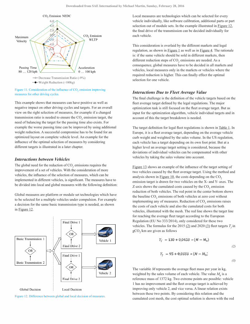
Figure 11. Consideration of the influence of CO2 emission improving measures for other driving cycles.

This example shows that measures can have positive as well as negative impact on other driving cycles and targets. For an overall view on the right selection of measures, for example if a changed transmission ratio is needed to ensure the CO2 emission target, the need of balancing the target for the passing time also exists. For example the worse passing time can be improved by using additional weight reduction. A successful compromise has to be found for an optimized layout on complete vehicle level. An example for the influence of the optimal selection of measures by considering different targets is illustrated in a later chapter.

Interactions between VehiclesThe global need for the reduction of CO2 emissions requires the improvement of a set of vehicles. With the consideration of more vehicles, the influence of the selection of measures, which can be implemented in different vehicles, is significant. The measures have to be divided into local and global measures with the following definition:

Global measures are platform or module set technologies which have to be selected for a multiple vehicles under compulsion. For example a decision for the same basic transmission type is needed, as shown in Figure 12.

Figure 12. Difference between global and local decision of measures.

Local measures are technologies which can be selected for every vehicle individually, like software calibration, additional parts or part selection out of module sets. In the example illustrated in Figure 12, the final drive of the transmission can be decided individually for each vehicle.

This consideration is overlaid by the different markets and legal regulation, as shown in Figure 1 as well as in Figure 4. The rationale is: if the same vehicle should be sold in different markets, then different reduction steps of CO2 emissions are needed. As a consequence, global measures have to be decided in all markets and vehicles, local measures only in the markets or vehicles where the required reduction is higher. This can finally effect the optimal selection for one vehicle.

Interactions Due to Fleet Average ValueThe final challenge is the definition of the vehicle targets based on the fleet average target defined by the legal regulations. The major optimization task is still focused on the fleet average target. But as input for the optimization algorithm, vehicle individual targets and in account of this the target breakdown is needed.

The target definition for legal fleet regulations is shown in Table 1. In Europe, it is a fleet average target, depending on the average vehicle curb weight and weighted by the sales volume. In the US regulation, each vehicle has a target depending on its own foot print. But at a higher level an average target setting is considered, because the deviations of individual vehicles can be compensated with other vehicles by taking the sales volume into account.

Figure 13 shows an example of the influence of the target setting of two vehicles caused by the fleet average target. Using the method and analysis shown in Figure 10, the costs depending on the CO2 emission target is drawn for two vehicles on the X- and Y- axes. The Z-axis shows the cumulated costs caused by the CO2 emission reduction of both vehicles. The red point in the center bottom shows the baseline CO2 emissions of both vehicles at zero cost without implementing any of measures. Reduction of CO2 emissions raises the costs of each vehicle and also the cumulated costs for both vehicles, illustrated with the mesh. The red line shows the target line for reaching the average fleet target according to the European Regulation (EU No 333/2014), only considered for these two vehicles. The formulas for the 2015 (2) and 2020 (3) fleet targets Tf in gCO2/km are given as follows

(2)

(3)

The variable M represents the average fleet mass per year in kg, weighted by the sales volume of each vehicle. The value M0 is a reference mass of 1372 kg. Two extreme points are possible: vehicle 1 has no improvement and the fleet average target is achieved by improving only vehicle 2, and vice versa. A linear relation exists between these two points. By considering this relation and the cumulated cost mesh, the cost optimal solution is shown with the red

Downloaded from SAE International by Michael Martin, Sunday, February 28, 2016

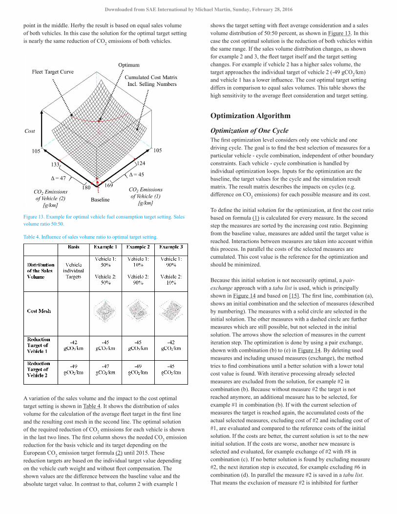
point in the middle. Herby the result is based on equal sales volume of both vehicles. In this case the solution for the optimal target setting is nearly the same reduction of CO2 emissions of both vehicles.

Figure 13. Example for optimal vehicle fuel consumption target setting. Sales volume ratio 50:50.

Table 4. Influence of sales volume ratio to optimal target setting.

A variation of the sales volume and the impact to the cost optimal target setting is shown in Table 4. It shows the distribution of sales volume for the calculation of the average fleet target in the first line and the resulting cost mesh in the second line. The optimal solution of the required reduction of CO2 emissions for each vehicle is shown in the last two lines. The first column shows the needed CO2 emission reduction for the basis vehicle and its target depending on the European CO2 emission target formula (2) until 2015. These reduction targets are based on the individual target value depending on the vehicle curb weight and without fleet compensation. The shown values are the difference between the baseline value and the absolute target value. In contrast to that, column 2 with example 1

shows the target setting with fleet average consideration and a sales volume distribution of 50:50 percent, as shown in Figure 13. In this case the cost optimal solution is the reduction of both vehicles within the same range. If the sales volume distribution changes, as shown for example 2 and 3, the fleet target itself and the target setting changes. For example if vehicle 2 has a higher sales volume, the target approaches the individual target of vehicle 2 (-49 gCO2/km) and vehicle 1 has a lower influence. The cost optimal target setting differs in comparison to equal sales volumes. This table shows the high sensitivity to the average fleet consideration and target setting.

Optimization Algorithm

Optimization of One CycleThe first optimization level considers only one vehicle and one driving cycle. The goal is to find the best selection of measures for a particular vehicle - cycle combination, independent of other boundary constraints. Each vehicle - cycle combination is handled by individual optimization loops. Inputs for the optimization are the baseline, the target values for the cycle and the simulation result matrix. The result matrix describes the impacts on cycles (e.g. difference on CO2 emissions) for each possible measure and its cost.

To define the initial solution for the optimization, at first the cost ratio based on formula (1) is calculated for every measure. In the second step the measures are sorted by the increasing cost ratio. Beginning from the baseline value, measures are added until the target value is reached. Interactions between measures are taken into account within this process. In parallel the costs of the selected measures are cumulated. This cost value is the reference for the optimization and should be minimized.

Because this initial solution is not necessarily optimal, a pair-exchange approach with a tabu list is used, which is principally shown in Figure 14 and based on [15]. The first line, combination (a), shows an initial combination and the selection of measures (described by numbering). The measures with a solid circle are selected in the initial solution. The other measures with a dashed circle are further measures which are still possible, but not selected in the initial solution. The arrows show the selection of measures in the current iteration step. The optimization is done by using a pair exchange, shown with combination (b) to (e) in Figure 14. By deleting used measures and including unused measures (exchange), the method tries to find combinations until a better solution with a lower total cost value is found. With iterative processing already selected measures are excluded from the solution, for example #2 in combination (b). Because without measure #2 the target is not reached anymore, an additional measure has to be selected, for example #1 in combination (b). If with the current selection of measures the target is reached again, the accumulated costs of the actual selected measures, excluding cost of #2 and including cost of #1, are evaluated and compared to the reference costs of the initial solution. If the costs are better, the current solution is set to the new initial solution. If the costs are worse, another new measure is selected and evaluated, for example exchange of #2 with #8 in combination (c). If no better solution is found by excluding measure #2, the next iteration step is executed, for example excluding #6 in combination (d). In parallel the measure #2 is saved in a tabu list. That means the exclusion of measure #2 is inhibited for further

Downloaded from SAE International by Michael Martin, Sunday, February 28, 2016

iteration steps. To show this effect, #2 is now filled in gray. The order for excluding measures in each iteration step is dependent on the cost impact. Cost-intensive measures are varied first, low-cost measures later. The iteration and optimization terminates when all measures were excluded once.

Figure 14. Principle of pair exchange optimization.

Optimization of Vehicle and FleetThe second optimization level handles vehicles as well as the fleet. In comparison to the first cycle-based optimization, more than one target is considered. Hereby a fleet consists of a set of vehicles and one vehicle consists of a set of targets. Based on this abstraction the only difference between considering one vehicle or multiple vehicles is the total number of targets. The optimization problem remains the same.

A balancing between different targets (CO2 emissions and driving performance) is required. To handle the vehicle as well as the fleet optimization, a genetic optimization method was implemented. The principle of a genetic method is shown in Figure 15 and based on [16]. The initial state is set by using the baseline values of the vehicles - meaning without any selection of measures. This represents the first parent generation. Every parent generates a defined number of child generations. For each child, one unused measure is selected and fixed in place, depending on a weighted random selection. The weighting is based on the impact of the measures. If a measure has an influence on many vehicles (global measures), it will be preferred. The selection process has the choice between including or excluding the selected measure. With this new selection of measures the statuses for all cycles for the children are updated, including the interaction analysis for the measures. Here the algorithm splits up into two paths. If all targets of a certain child are reached, then this child is defined as a final solution. If not all targets are reached, then the algorithm verify the reachability of the remaining target individually, by using the cycle-based optimization. This investigation is needed, because if too many measures are excluded in the iteration steps, targets can be not reached anymore. If that is the case, the concerned child will be excluded for further investigation. For the other children of the current generation, a Pareto front is generated. Figure 16 illustrates a Pareto front. The dots represent all children solutions defined by two parameters. The first parameter on the X axis are the actual costs CF based on equation (4). The absolute costs of a child are the sum of the costs c of the already included measures m weighted by the sales

volume sv of each measure. The second parameter on the Y axis describes the result of the target function for the optimization described by equation (5). The target function TF calculates and cumulates the differences between the actual statuses s and the target values t in relation to the baseline value bl of all considered test cycles tc and vehicles v.

(4)

(5)

The purpose of the optimization is to minimize the result of this target function to zero. A value of zero means that all targets are reached for a certain child. The Pareto front is a set of children (solutions) defined as follows: a solution s belongs to the Pareto front if and only if there is no other solution s’ for which the value of the target function and the costs are both smaller than the respective values corresponding to solution s. Primarily the two extreme points of the Pareto front are selected, the child with the lowest cost and the child with the lowest result of the target function. Secondary out of this Pareto front a defined number of children are chosen by a random selection. The selected children represent the new parent solution for the next iteration step.

Open to allow the change of measures already decided, a mutation is included additionally. This mutation randomly changes single measures and evaluates if a better solution can be found by changing.

Figure 15. Principle of the genetic optimization.

Downloaded from SAE International by Michael Martin, Sunday, February 28, 2016

Figure 16. Example of a Pareto front.

In each iteration step one selected measure will become unchangeable. Each additional iteration will add another unchangeable measure, e.g. in the first iteration one measure will be fixed, in the second two measures etc. This means that the maximum number of iterations is equal to the number of measures. The algorithm terminates if a defined number of final solutions is found. Final solutions means children with a result for the target function of zero. Out of all solutions, the child with the lowest cost is selected as optimal solution.

Case Study

Influence of Cycle, Vehicle and Fleet Based OptimizationFigure 5 showed the different optimization levels: cycle, vehicle and fleet based. The result of a case study due the comparison between this three levels is shown in Table 5. The columns are divided into this three optimization levels and their results. The upper part of the table shows a set of defined measures. For a better overview only these measures are listed in the table, which were selected by the optimization algorithm. Also other measures for improving CO2 emissions were considered, but not shown in the table. The fields show two states: An empty field means that the corresponding measure is not included in the optimal solution. In contrast an “X” means that this measure is included. Additional brackets mean that the corresponding measure is global. The measures represent typical technologies for improving CO2 emissions. Hereby the intention of this case study is to show the method. Final results will depend on the technologies, cost and vehicles etc. The middle part of the table shows the resulting cost relation between all three solutions. In the bottom part the test cycles, their targets and the results of the test cycles due to the selection of measures are shown.

The cycle based optimization in the first column only considers the NEDC cycle of the selected vehicle. The other three tests are not considered and due to this the results are market with brackets. This optimization result represents the best solution for the vehicle, focused on CO2 emissions, and is defined as reference for the vehicle and fleet based optimization.

The vehicle level in the second column considers further boundary constraints for acceleration, passing time and maximum speed. The advantages and disadvantages of measures with respect to other cycles and also the achievement of the corresponding targets have to be balanced by the optimization. So the combination of measures

found to be the best in the vehicle based optimization level differs from the best combination found in the cycle based level. The selection of measures is not optimal for the NEDC itself anymore and so the cost for the updated selection of measures increases. As seen in the table, the difference is resulted by the passing time from 80 to 120 kph. In the cycle based optimization, the passing time is a not considered spillover and the target of 12.0 seconds was not reached. If this boundary constraint and target is considered in the vehicle optimization level, then the selection of measures changes. In this case the adaption of the transmission was not selected anymore, because on the one hand it improves CO2 emissions but on the other hand it has negative impact on driving performance. In order to reach the target of CO2 emissions, other measures (aerodynamic and alternator improvement) have to be selected. The resulting selection is not optimal for the NEDC itself and so the cost can increase, in this example at around 20%.

Table 5. Influence of optimal measure selection due to boundary constraints and global view.

Downloaded from SAE International by Michael Martin, Sunday, February 28, 2016

In a further step the correlation to a fleet is considered in the third column. In this case the considered fleet consists of five vehicles. Hereby the classification of global and local measures becomes important. In Table 4 the global measures are marked with brackets. For example the global “Aerodynamic Measure #3” is not optimal for the overall fleet and is not selected for this particular vehicle anymore. In order to reach all targets, other local measures now have to be defined for the selected vehicle. This results in additional costs compared to the cycle-based optimization.

This fictitious example shows the impact of the complete vehicle considerations and the necessary interactions to a fleet. Of course it is possible to design a vehicle cost optimal for a certain cycle, but the need to consider other targets for driving performance and drivability as well as the overlaid platform and fleet strategies is important. The optimization method presented here is able to deal with this complex problem and yields valuable input for the vehicle development.

Sensitivity AnalysisA question with respect to the quality of the solution is the robustness of the method. A mathematical optimization method can be effective to find the optimal solution, but in the end the quality of the solution directly depends on the input data. Based on the fixed input values, the algorithm tries to find the global optimal solution. In the context of the vehicle development it is difficult to ensure the availability of accurate input data for the simulation, especially in early development stages. It will be not possible to define precise values as input for the mathematical optimization. Hence, simulation results and cost information will result in tolerances. Input value for the optimization changes when for example a cost value changes or simulation results differs from test results. Performing the optimization with the changed input data would result in a new optimal solution eventually.

To ensure a robust result for the vehicle development, an additional sensitivity analysis was done for the reference vehicle shown in Figure 17. The sensitivity analysis is overlaid on the optimization algorithm results. It varies the input data for the optimization and evaluates the changes. Figure 17 shows a waterfall diagram with a set of selected measures, optimized until the target value is reached. On the right side further measures are noted, which would further improve CO2 emissions, but not selected for the optimal solution. To check the robustness of the method and the results, a sensitivity analysis was done. For that, as shown with the arrows, the values for improvement and costs were increased or decreased. New optimization loops were performed and analyzed with modified values. The results were compared with the initial solution and measures changed or updated in the process. In some cases other optimal solutions were obtained. The dark green filled bars show measures which were always selected. The light green striped and yellow dotted bars, showing percentage data, are measures that were included or excluded in the optimal selection depending on the input data. The percentage describes how often the measures were selected. The gray bars represent measures never used.

Figure 17. Sensitivity analysis for an optimal solution.

The results of this example is that in 87% of the variation cases the optimal solution was reproducible. Six out of eight measures were always used. In less than 13% of the variations the last two measures were partly replaced by two other measures. The result of the sensitivity analysis can be used to evaluate the robustness due to the input data and to interpret as a trend analysis which combination of measures is the steadiest one.

Summary / ConclusionsThe presented research showed a mathematical approach to handle future CO2 emission fleet targets for supporting a vehicle development process. Because of more demanding targets in the future, the importance of cost considerations increases. Additional technologies have to be developed and implemented into the vehicles and the fleet.

For the right selection of such measures, a systematic and holistic approach for cost handling and optimization will become inevitable.

To evaluate the influence of measures regarding CO2 emissions, a simulation model is needed. The structure of this model as well as an automated environment was shown. The automation of the simulation is needed to handle the huge simulation matrix of vehicle, cycles and measures. The information of cost and influence of the defined measures is the input for the optimization. Hereby the optimization is divided into different parts. The challenges and requirements for the optimization method were explained. Interactions between measures, balancing of vehicle targets and the average fleet target setting have to be handled. For the consideration of one cycle and one vehicle a pair exchange method with tabu list was used. The extended optimization method for the whole fleet is based on a genetic algorithm with mutation.

Finally the benefits of the presented optimization approach were demonstrated on a case study. Usually studies for improving CO2 emissions of vehicles are based on one detailed vehicle or on rough statements on fleet level. The presented methodic combines both considerations. The need of this holistic combined consideration of individual vehicles with the fleet background was shown. Thereby different optimization results and the different selection of measures due to the optimization levels were shown. The optimal selection of measures differs if only a cycle, a vehicle or a fleet is considered.

Downloaded from SAE International by Michael Martin, Sunday, February 28, 2016

This result confirmed the need of a holistic approach to handle the target achievement of future legal CO2 emission regulation including the consideration of cost. The cooperation between a detailed evaluation of the vehicles and the fleet consideration is needed to find the overall best solution.

Due to the limited access and availability of detailed input data during early development phases, the usage of a sensitivity analysis to evaluate the robustness of the solution was shown in the second example. Input data can change during the development time of a vehicle. To prevent a change in solutions during a vehicle development project, the robustness of the approach should be verified. As presented, one possible method is a sensitivity analysis to check the reproducibility of the solution if input data changes. In the presented case study a steady solution was proved with the sensitivity analysis.

The planned next steps of the work is the extension of the fictitious fleet with a higher number of vehicles. Hereby the further validation of the optimization method as well as the proof of the robustness of the solution is the focus.

References1. “Das Kyoto-Protokoll - Ein Meilenstein für den Schutz des

Weltklimas.“ (Bundesministerium für Umwelt, Naturschutz und Reaktorsicherheit, 2005).

2. Lunanova, M.: „Optimierung von Nebenaggregaten -Maßnahmen zur Senkung der CO2-Emissionen von Kraftfahrzeugen.“ (Vieweg+Teubner, 2009), 3, DOI: 10.1007/978-3-8348-9603-2.

3. Wallentowitz, H., Freialdenhoven, A. and Olschewski, I.: „Strategien in der Automobilindustrie - Technologietrends und Marktentwicklung.“ (Vieweg+Teubner, 2009), 11, DOI: 10.1007/978-3-8348-9311-6.

4. Bandivadekar, A., Cheah, L., Evans, C., Grodde, T., Heywood, J., Kasseris, E., Kromer, M. and Weiss, M.: “Reducing the fuel use and greenhouse gas emissions of the US vehicle fleet.” Elsevier - Energy Policy, 2008, 2754-2760, DOI: 10.1016/j.enpol.2008.03.029.

5. Cheah, L. and Heywood, J.: “Meeting U.S. passenger vehicle fuel economy standards in 2016 and beyond.” Elsevier - Energy Policy, 2011, 454-466, DOI: 10.1016/j.enpol.2010.10.027.

6. “CO2-Reduzierungspotentiale bei PKW bis 2020.“ (Bundesministerium für Wirtschaft und Technologie, 2012).

7. “Technologies to improve light-duty vehicle fuel economy.” (Energy and Environmental Analysis, INC., 2007).

8. Fontaras, G. and Samaras, Z.: “On the way to 130 g CO2/kmestimating the future characteristics of the average european passenger car.” Elsevier - Energy Policy, 2010, 1826-1833, DOI: 10.1016/j.enpol.2009.11.059.

9. Silva, C., Ross, M. and Farias, T.: “Analysis and simulation of low-cost strategies to reduce fuel consumption and emissions in conventional gasoline light-duty vehicles.” Elsevier - Energy Conversion and Management, 2009, 215-222, DOI: 10.1016/j.enconman.2008.09.046.

10. Tscharnuter, D.: „Optimale Auslegung des Antriebsstrangs von Kraftfahrzeugen - Modellbildung, Simulation und Optimierung.“ Ph.D. thesis, Department of Mathematics, University of Technology, Munich, 2000.

11. Martin, M.: “Reduction of CO2 emissions - Optimization approach: vehicle vs. fleet”. Proceedings of the 15th Stuttgart International Symposium: volume 1, 595 - 608, 2015, ISBN: 978-3-658-08844-6.

12. Martin, M., Premstaller, R. and Eichberger, A.: “Virtual Optimisation of Fleet Consumption under Cost Consideration”. ATZ - Automobiltechnische Zeitschrift, 74-80, April 2015, DOI: 10.1007/s35148-015-0017-6.

13. Gamsjäger, C., Hager, J., Kordesch, V. and Öller, W.: “Intelligent heat management - a chance for further reduction of emissions and fuel consumption.” Proceedings of the Aachen Colloquium - Automobile and Engine Technology: 871-888, 2012.

14. Fleckner, M., Göhring M., and Spiegel, L.: “Neue Strategien zur verbrauchsoptimalen Auslegung der Betriebsführung von Hybridfahrzeugen.“ Proceedings of the Aachen Colloquium - Automobile and Engine Technology: 681-708, 2009.

15. Glover, F. W. and Laguna, M.: “Tabu Search“.

16. Schumacher, A.: “Optimierung mechanischer Strukturen. Second Edition.” (Springer, 2013), 94-99, DOI: 10.1007/978-3-642-34700-9-4.

Contact InformationMichael Martin, Magna Steyr Engineering AustriaDepartment Complete Vehicle / Energy Management & Drivabilitym.martin@magna.comwww.magnasteyr.com

AcknowledgmentsThe author thanks the Austrian BMVIF and FFG for sponsoring this work and doctor thesis within the scope of “talents” and “mobility of the future”. Additionally the author thanks Robert Premstaller, representative for Magna Steyr Engineering Austria, for the support of this doctor thesis.

Definitions/Abbreviations1D - 1 Dimensional

ACEA - European Automobile Manufacturers’ Association

CN - China

CO2 - Carbon Dioxide

EU - European Union

FTP - Federal Test Procedure

GHG - Greenhouse Gas

HWFET - Highway Fuel Economy Test

ICE - Internal Combustion Engine

JC08 - Japanese Chassis Dynamometer Test

NEDC - New European Driving Cycle

WLTP - World Harmonized Light Vehicle Test Procedure

Downloaded from SAE International by Michael Martin, Sunday, February 28, 2016

The Engineering Meetings Board has approved this paper for publication. It has successfully completed SAE’s peer review process under the supervision of the session organizer. The process requires a minimum of three (3) reviews by industry experts.

All rights reserved. No part of this publication may be reproduced, stored in a retrieval system, or transmitted, in any form or by any means, electronic, mechanical, photocopying, recording, or otherwise, without the prior written permission of SAE International.

Positions and opinions advanced in this paper are those of the author(s) and not necessarily those of SAE International. The author is solely responsible for the content of the paper.

ISSN 0148-7191

http://papers.sae.org/2016-01-0904

Downloaded from SAE International by Michael Martin, Sunday, February 28, 2016