Optimization and validation of pumping system design and ...
44
Optimization and Engineering (2021) 22:643–686 https://doi.org/10.1007/s11081-020-09553-4 RESEARCH ARTICLE Optimization and validation of pumping system design and operation for water supply in high-rise buildings Tim M. Müller 1 · Philipp Leise 1 · Imke-Sophie Lorenz 1 · Lena C. Altherr 2 · Peter F. Pelz 1 Received: 31 October 2019 / Revised: 10 August 2020 / Accepted: 13 August 2020 / Published online: 19 September 2020 © The Author(s) 2020 Abstract The application of mathematical optimization methods for water supply system design and operation provides the capacity to increase the energy efficiency and to lower the investment costs considerably. We present a system approach for the optimal design and operation of pumping systems in real-world high-rise buildings that is based on the usage of mixed-integer nonlinear and mixed-integer linear modeling approaches. In addition, we consider different booster station topologies, i.e. parallel and series- parallel central booster stations as well as decentral booster stations. To confirm the validity of the underlying optimization models with real-world system behavior, we additionally present validation results based on experiments conducted on a modu- larly constructed pumping test rig. Within the models we consider layout and control decisions for different load scenarios, leading to a Deterministic Equivalent of a two- stage stochastic optimization program. We use a piecewise linearization as well as a piecewise relaxation of the pumps’ characteristics to derive mixed-integer linear models. Besides the solution with off-the-shelf solvers, we present a problem specific exact solving algorithm to improve the computation time. Focusing on the efficient exploration of the solution space, we divide the problem into smaller subproblems, which partly can be cut off in the solution process. Furthermore, we discuss the perfor- mance and applicability of the solution approaches for real buildings and analyze the technical aspects of the solutions from an engineer’s point of view, keeping in mind the economically important trade-off between investment and operation costs. B Tim M. Müller [email protected] Peter F. Pelz [email protected] 1 Chair of Fluid Systems, Department of Mechanical Engineering, Technische Universität Darmstadt, Darmstadt, Germany 2 Faculty of Energy, Building Services and Environmental Engineering, Münster University of Applied Sciences, Stegerwaldstr. 39, Steinfurt, Germany 123
Transcript of Optimization and validation of pumping system design and ...

Optimization and Engineering (2021) 22:643–686https://doi.org/10.1007/s11081-020-09553-4
RESEARCH ART ICLE
Optimization and validation of pumping system design andoperation for water supply in high-rise buildings
Tim M. Müller1 · Philipp Leise1 · Imke-Sophie Lorenz1 · Lena C. Altherr2 ·Peter F. Pelz1
Received: 31 October 2019 / Revised: 10 August 2020 / Accepted: 13 August 2020 /Published online: 19 September 2020© The Author(s) 2020
AbstractThe application ofmathematical optimizationmethods for water supply system designand operation provides the capacity to increase the energy efficiency and to lower theinvestment costs considerably. We present a system approach for the optimal designand operation of pumping systems in real-world high-rise buildings that is based onthe usage of mixed-integer nonlinear and mixed-integer linear modeling approaches.In addition, we consider different booster station topologies, i.e. parallel and series-parallel central booster stations as well as decentral booster stations. To confirm thevalidity of the underlying optimization models with real-world system behavior, weadditionally present validation results based on experiments conducted on a modu-larly constructed pumping test rig. Within the models we consider layout and controldecisions for different load scenarios, leading to a Deterministic Equivalent of a two-stage stochastic optimization program. We use a piecewise linearization as well asa piecewise relaxation of the pumps’ characteristics to derive mixed-integer linearmodels. Besides the solution with off-the-shelf solvers, we present a problem specificexact solving algorithm to improve the computation time. Focusing on the efficientexploration of the solution space, we divide the problem into smaller subproblems,which partly can be cut off in the solution process. Furthermore, we discuss the perfor-mance and applicability of the solution approaches for real buildings and analyze thetechnical aspects of the solutions from an engineer’s point of view, keeping in mindthe economically important trade-off between investment and operation costs.
B Tim M. Mü[email protected]
Peter F. [email protected]
1 Chair of Fluid Systems, Department of Mechanical Engineering, Technische UniversitätDarmstadt, Darmstadt, Germany
2 Faculty of Energy, Building Services and Environmental Engineering, Münster University of AppliedSciences, Stegerwaldstr. 39, Steinfurt, Germany
123

644 T. M. Müller et al.
Keywords Technical Operations Research · MINLP · MILP · Experimentalvalidation · Pumping systems · Water supply systems
1 Introduction
More than half of the world’s population (55%) lived in urban areas in 2018, as shownin UN (2018). Based on this data published by the United Nations, it is estimated that2.5 billion people will be added to the urban population by 2050 leading to an increaseby more than half of the number of people living in urban areas today. This continuoustrend towards urbanization will lead to an increasing number of mega-cities, citieswith more than 10 million inhabitants.
As the space for living in cities is limited, one effective way to cope with the steadyurbanization and to create living space are high-rise buildings. In those buildingsdistributed pressure boosting pumping stations, also called booster stations, providewater for every floor, especially in higher pressure zones. Consequently, their needwillincrease proportionally with the number of high-rise buildings. Already today thereis a rapid growth of completed buildings of 200 meters or greater height, CTBUH(2018).
Water supply systems are a key component of any urban infrastructure, cf. Coelhoand Andrade-Campos (2014), and urbanization will pose increasing challenges forthese infrastructures in the future: Whilst a secure supply of water for the growingnumber of citizens is to be ensured, energy consumption for water supply must bereduced on the way to a more sustainable future. Thus, efficiency optimization ofwater supply systems has been in the focus of ongoing research, for a review cf. e.g.Coelho and Andrade-Campos (2014).
While existing research has so far tended to focus on the energy consumption oflarger centralized water infrastructures, in this contribution, we want to investigatethe energy consumption of the mentioned booster stations for buildings. Especially intall buildings, booster stations have a considerable energy consumption, in particularif they are wrongly dimensioned and/or operated. Therefore, the potential for energysavings through the application of several pressure zones or a decentralized pumpplacement and an optimal selection of pump types is high, cf. e.g. Altherr et al. (2019).
In order to unlock this optimizationpotential, a large number of pipenetwork topolo-gies and pump configurations must be considered in the planning process. However,with the increasing number of degrees of freedom, especially in tall buildings, it is adifficult challenge to investigate all possible system variants, as the number of possibledesign choices can be overwhelming. Moreover, one not only has to check whether apromising design is able to fulfill the different load scenarios occurring in the building,but also for an economic solution by balancing investment and operating costs againsteach other. To achieve these goals, we present an optimization-aided system designapproach based on a problem-specific solving algorithm. In order to ensure that theunderlying optimization models represent the system under consideration with suf-ficient accuracy, we also present an experimental validation. To model the pressurelosses due to friction we use own measurements as well as literature data and comparethe optimization results of both approaches.
123

Optimization and validation of pumping systems 645
In the following Sect. 2, we introduce relevant literature for the optimization. After-wards, we present the technical application in detail and show different formulationsof the optimization model as well as a problem specific solving algorithm. We thendiscuss the performance of different solving approaches as well as technical aspects ofthe solutions and close with an experimental validation. Finally we draw a conclusionand give an outlook for future work.
2 Related work
In this article we present a holistic approach to the optimal synthesis of technicalsystems, which we illustrate by means of a pumping system for water supply. In thecontext of this research focus, the state-of-the-art is presented in two different areas:
(i) Methods used in engineering for the design and efficiency optimization of pumpingsystems, in particular pressure boosting systems in buildings.
(ii) Application of mathematical optimization methods to general technical systems,in particular methods for two-stage optimization problems.
In the next two subsections we will give a short overview of relevant literature inthese two areas.
2.1 Design and efficiency optimization of pumping systems
When optimizing the efficiency of a pumping system, a first step is to assemble thesystem from efficient components. For the transport of drinking water, booster stationsconsisting of centrifugal pumps are commonly used. Therefore, we focus on this pumptype within this literature overview.
The development and hydraulic optimization of centrifugal pumps is already at avery high level and multiple standard works are focusing on centrifugal pump designas well as performance, cf. e.g. Japikse and Marscher (1997), Brennen (2011), orGülich (2010). In recent decades, also through the use of computer-aided methodssuch as Computational Fluid Dynamics (CFD), cf. e.g. Garg (1998), the efficiency ofcentrifugal pumps, in particular at their design point, has been continuously improved.
In real life applications, however, it can be seen that centrifugal pumps are predom-inantly not operated at their design point, but in the partial load range for a large part ofthe time, cf. Hirschberg (2014). In this case, the excess energy is either dissipated viathrottling valves, or—if variable speed pumps, so called RPM-regulated pumps, areemployed—they are operated at a lower rotational speed than their nominal rotationalspeed. Both leads to an operation at lower efficiency, often far away from their bestefficiency point. Therefore, when classifying and optimizing pump performance, asuitable approach for assessing efficiency in practical usage is crucial.
The product approach, which is part of an european standard for energy-efficiencyevaluation of water pumps, c.f. EN 16480:2016 (2016), is a first step in this direction.This approach no longer considers merely the pump as a component, but the pump andelectric motor as part of a system. The efficiency of this system is assessed accordingto the Minimum Energy Efficiency Index (MEI) which rates the pump’s efficiency not
123
646 T. M. Müller et al.
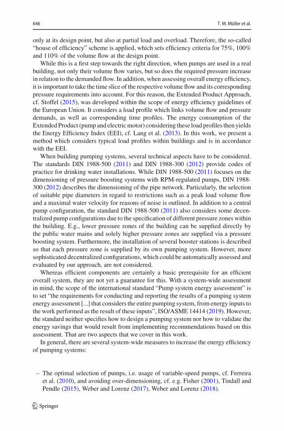
only at its design point, but also at partial load and overload. Therefore, the so-called“house of efficiency” scheme is applied, which sets efficiency criteria for 75%, 100%and 110% of the volume flow at the design point.
While this is a first step towards the right direction, when pumps are used in a realbuilding, not only their volume flow varies, but so does the required pressure increasein relation to the demanded flow. In addition, when assessing overall energy efficiency,it is important to take the time slice of the respective volume flow and its correspondingpressure requirements into account. For this reason, the Extended Product Approach,cf. Stoffel (2015), was developed within the scope of energy efficiency guidelines ofthe European Union. It considers a load profile which links volume flow and pressuredemands, as well as corresponding time profiles. The energy consumption of theExtendedProduct (pump and electricmotor) considering these load profiles then yieldsthe Energy Efficiency Index (EEI), cf. Lang et al. (2013). In this work, we present amethod which considers typical load profiles within buildings and is in accordancewith the EEI.
When building pumping systems, several technical aspects have to be considered.The standards DIN 1988-500 (2011) and DIN 1988-300 (2012) provide codes ofpractice for drinking water installations. While DIN 1988-500 (2011) focuses on thedimensioning of pressure boosting systems with RPM-regulated pumps, DIN 1988-300 (2012) describes the dimensioning of the pipe network. Particularly, the selectionof suitable pipe diameters in regard to restrictions such as a peak load volume flowand a maximal water velocity for reasons of noise is outlined. In addition to a centralpump configuration, the standard DIN 1988-500 (2011) also considers some decen-tralized pump configurations due to the specification of different pressure zones withinthe building. E.g., lower pressure zones of the building can be supplied directly bythe public water mains and solely higher pressure zones are supplied via a pressureboosting system. Furthermore, the installation of several booster stations is describedso that each pressure zone is supplied by its own pumping system. However, moresophisticated decentralized configurations, which could be automatically assessed andevaluated by our approach, are not considered.
Whereas efficient components are certainly a basic prerequisite for an efficientoverall system, they are not yet a guarantee for this. With a system-wide assessmentin mind, the scope of the international standard “Pump system energy assessment” isto set “the requirements for conducting and reporting the results of a pumping systemenergy assessment [...] that considers the entire pumping system, from energy inputs tothe work performed as the result of these inputs”, ISO/ASME 14414 (2019). However,the standard neither specifies how to design a pumping system nor how to validate theenergy savings that would result from implementing recommendations based on thisassessment. That are two aspects that we cover in this work.
In general, there are several system-widemeasures to increase the energy efficiencyof pumping systems:
– The optimal selection of pumps, i.e. usage of variable-speed pumps, cf. Ferreiraet al. (2010), and avoiding over-dimensioning, cf. e.g. Fisher (2001), Tindall andPendle (2015), Weber and Lorenz (2017), Weber and Lorenz (2018).
123

Optimization and validation of pumping systems 647
– The allocation of several pressure zoneswithin the building and the usage of decen-tralized pump layouts, cf. e.g. Norgaard and Nielsen (2010); Leise and Altherr(2018).
– The optimization of the pumps’ operation, cf. e.g. Pedersen andYang (2008), Großet al. (2017), and Nowak et al. (2018).
The approach presented in this contribution allows to cover all three of these aspects,since not only the optimal pumping system design, but also its optimal operation canbe considered.
While in this work we particularly focus on the optimization of the efficiency andinvestment costs, other possible objectives are shown in the literature. One example isthe optimization of resilient water supply networks as shown by Herrera et al. (2016),Hartisch et al. (2018), and Altherr et al. (2019).
2.2 Mathematical aspects of two-stage optimization problems in engineering
Besides literature from the engineering domain covering the technical aspects of opti-mizing pumping systems, also previous works regarding the mathematical aspects arerelevant.
When designing an economically optimal pumping system, the overall goal oftenis to minimize the sum of investment costs and energy costs for the expected life cycle.Since the loadwithin residential buildings varies, cf. Sect. 2.1, its operation at differentload points has to be considered to assess the energy costs of the pumping system.
The correspondingmathematical optimization problemconsists of two stages: First,finding a low-priced investment decision, i.e. a pump and pipe configuration. Second,operating a subset of the chosen pumps for each quasi-stationary demand scenario ofthe given load profile, such that the system satisfies this demand and at the same timethe efficiency is maximized.
In this case, the considered load profile can be seen as a discrete distribution ofuncertain load parameters, with the time portion of each load scenario corresponding toits probability of occurrence. The optimization program, which minimizes investmentcosts as well as expected value of operation costs, can then be seen as the DeterministicEquivalent of a general two-stage stochastic program with recourse, cf. e.g. Wets(1974).
As many optimization problems in the area of engineering design are subject touncertain parameters, e.g. uncertain material characteristics or load scenarios, two-stage stochastic programs have been frequently studied in this context, and a goodoverview can be found in Popela (2010) and Popela et al. (2014). The life cycle ofproducts and systems in engineering includes the two phases of planning (first stage)and operation (second stage). In two-stage stochastic optimization problems the oper-ation is already anticipated in the planning phase, which leads to better investmentdecisions. The operation itself is then typically ensured by closed- or open-loop con-trollers.
An important aspect for the difficulty of solving these two-stage optimization prob-lems to global optimality is whether integer variables are (1) present in the first stagesolely, or (2) also present in the second stage. Regarding design and operation opti-
123
648 T. M. Müller et al.
mization of technical systems, integer variables in the first stage, and more preciselybinary variables, are often used to model purchase decisions. Moreover, in this work,binary variables in the second stage are used to model the activation or deactivationof active components, i.e. an on/off-switch, leading to problems of case (2).
Theoretical aspects of these problems, also called complete mixed-integer recourseproblems, have e.g. been investigated by Schultz (1992), and sophisticated solutionapproaches have been proposed, cf. e.g. Carøe and Tind (1998). Given the formulationas Deterministic Equivalent Program, standard solution approaches based on Branch& Bound with LP relaxation may be applied. Yet these might suffer from high com-putation times, especially if multiple (load) scenarios are considered in the secondstage.
3 Technical application
As mentioned in the previous sections, we generate the Deterministic EquivalentPrograms of two-stage stochastic optimization models to compute energy-efficientcentralized and decentralized booster stations in high-rise buildings and validate thesemodels on a test rig. The physical properties of these systems and topology decisionsare modeled within the constraints of the optimization programs. Within this contri-bution, the fresh cold water supply is considered solely, while waste water, hot water,and water for firefighting are not considered. Thereby, the objective is to minimizethe simplified life-time cost, which consists of investment and energy costs within thelifetime. These two parts represent the economically most important goals, cf. Tolva-nen (2007), when designing pumping systems. When modeling these systems, twoaspects are of importance. First, reasonable computation times of model instances arerequired. Second, the model’s level of detail has to represent the real system with anacceptable accuracy to allow for the transfer of the optimization results. The computedoptimumwithin the model instance, should represent the true optimum of the underly-ing technical system. Usually, a trade-off between these two goals is necessary, as theformer tends to lead to models that are as simple as possible, while the latter demandsfor models that are highly accurate, but computationally not tractable. To achieve amodel that is as simple as possible and at the same time as accurate as needed, weconduct an experimental validation step based on a test rig that represents a scaledbuilding with five pressure zones.
We present all relevant basics of the pump and booster station modeling, the testrig, the system modeling and the preselection of pumps in the following subsections.
3.1 Pumpmodeling
The most important components to fulfill the water supply in high-rise buildings arethe pumps. All pumps are modeled with polynomial approximations for the pressure–volume flow characteristic, as well as the power–volume flow characteristic. Thisapproach is based on Ulanicki et al. (2008). We model the pressure increase Δp =f (q, n) with f : R+
0 × R+0 → R
+0 by using a quadratic approximation relating the
123
Optimization and validation of pumping systems 649
0 10 20 30 40 50VOLUME FLOW in m³/h
00 10 20 30 40 50
0
1
2
3
4
5
VOLUME FLOW in m³/h
POW
ER C
ON
SU
MPT
ION
in
kW
a b D
A EH
ER
US
SERP
Δin
bar
1
2
3
4
5
6
= 0.3
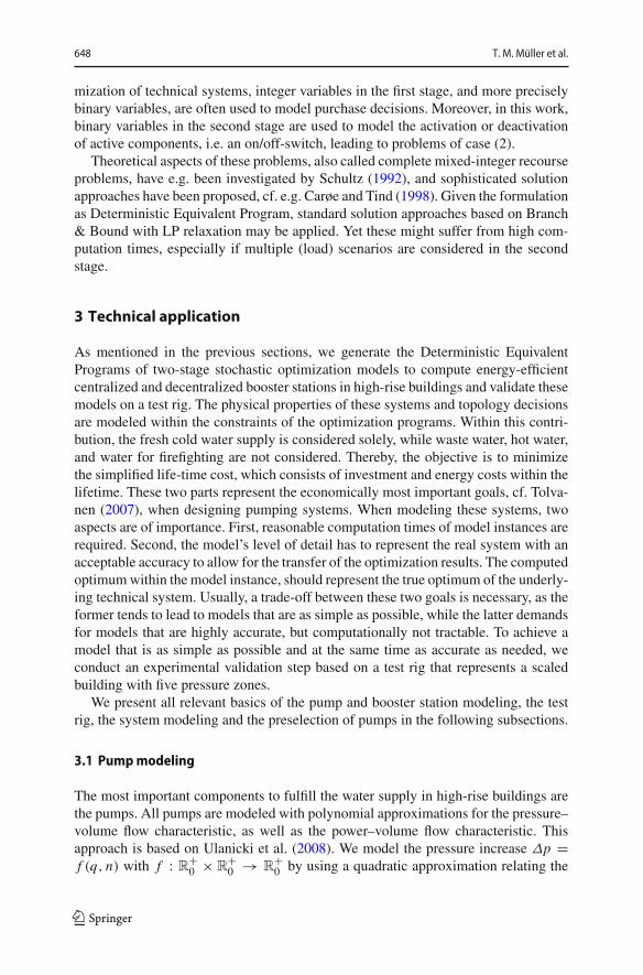
Fig. 1 Characteristics for an example pump based on the used pump model. These characteristics areusually limited in each domain according to specific pump requirements. The different curves describeseveral different rotational speeds
pressure head Δp, the volume flow q ∈ R+0 and the normalized rotational speed
n ∈ [N , N ], as given by
Δp =2∑
m=0
αm q 2−m nm, (1)
where the parameters αm and the lower bound of the normalized rotational speed Ndepend on the pump type. The rotational speed is normalized by using its maximumvalue. Therefore, we get an upper bound N = 1. For better readability, we refer tothe normalized rotational speed in the following as rotational speed or speed, only.The power po = g(q, n) with g : R+
0 × R+0 → R
+0 is modeled by using a cubic
approximation,
po =3∑
m=0
βm q 3−m nm . (2)
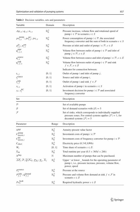
The parameters αm and βm are derived from manufacturer provided component char-acteristics for each pump type. Exemplified characteristic diagrams for a pump areshown in Fig. 1.
The shown characteristics are often limited bymaximumpower aswell asminimumand maximum volume flow requirements for each pump. These limits are added in theunderlying optimization as additional constraints to model a realistic pump behavior.For simplicity they are not shown in Fig. 1.
3.2 Booster stationmodeling
The function of a booster station is to provide sufficient pressure to overcome thegeodetic height of the floor to be provided with water as well as the friction in the pipesfeeding the respective floor. We distinguish three different booster station topologies,
123
650 T. M. Müller et al.
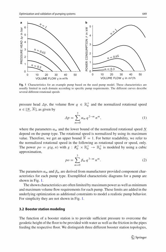
Fig. 2 Exemplified systemdesign of the underlyingoptimization program
which differ in the alignment of the considered pumps. Today, pumps are commonlyaligned in parallel at the lowest pressure zone of the building, as the product rangeof various manufacturers (Wilo 2020; KSB SE Co KGaA 2020; Grundfos PumpsLtd 2016) and the discussion in (Gülich 2010, pp. 666–669) shows. This leads to acentral, parallel booster station design providing the pressure and volume flow for thewhole building. Varying from this approach, also the serial arrangement of pumps in acentral booster station is possible, leading to higher degrees of freedom in the designprocess and therefore allowing for higher energy efficiency of the booster station. Forthe centralized topology the building’s demand can be modeled as solely one sinkwith one available water source. Additionally to these centralized system topologies,a decentralized booster station topology is possible. In this approach, pumps can bepositioned at any pressure zone of the building and therefore amore accurate modelingof the volume flow demand, i.e. the flow demand per pressure zone, is necessary. In thefollowing, we comprise floors of similar height into individual pressure zones. Eachpressure zone is modeled as an individual sink which has a different pressure demand,depending on the height of the floors. The decentralized topology allows for an evenhigher degree of freedom of pump arrangement and a reduction of the throttle losses,facilitating the improvement of the overall efficiency even further.
The system design approach with an exemplified booster station is shown in Fig. 2.In this exemplary system three pumps are used. The first pump is used in series withthe remaining two pumps. The second and third pump supply different pressure zonesin the building individually.
3.3 Test rig for validation
As indicated before, an experimental validation of the optimization results is crucial toguarantee the technical functionality. A validation using real buildings is not possiblefor reasons of high effort. In addition, novel concepts, i.e. the decentralized boosterstation design, shall be investigated, which cannot be realized in already existingbuildings.
123

Optimization and validation of pumping systems 651
Fig. 3 Sketch (left) and photo (right) of the modular test rig with a central booster station design
For this reason, a down-scaled, modular test rig has been set up, cf. Figure 3 andMüller et al. (2019b). The down-scaled system’s booster station has the same charac-teristics as those of high-rise buildings. The maximum geodetic height difference is5m divided into five different pressure zones, which can be supplied individually. Thewater is pumped from a tank with constant pressure to the five pressure zones by thebooster station.As in real buildings, thewater flows in at a constant supply pressure andflows out in an open drain pipe at ambient pressure (open system). The water returns tothe tank to keep the water level and therefore the supply pressure constant. The test rigis equipped with sensors for measuring the volume flow in each pressure zone as wellas the pressure head and power consumption of each pump. It is possible to control thespeed of the pumps and the valve position on each pressure zone and thus to controlthe volume flow on each pressure zone. Overall, a set of thirteen pumps, consisting ofsix different types, is available to build and test different booster station designs.
The pumps are centrifugal circulator pumps for heating systems with an integratedfrequency converter (FC) and therefore speed controllable. The sizes are chosen tofit the needs for the down-scaled booster system, even though the ratio of pressurehead to volume flow is lower than in real-world booster station pumps. The pumpscan be connected in any way and up to six pumps can be operated simultaneously as abooster station for the test rig. Compared to real pressure booster stations, the frictioncaused by installation fittings of the pumps (e.g. for pressure measurement) on the testrig is quite high. Therefore, those pressure losses are taken into account in the losscoefficient ζinst.
123
652 T. M. Müller et al.
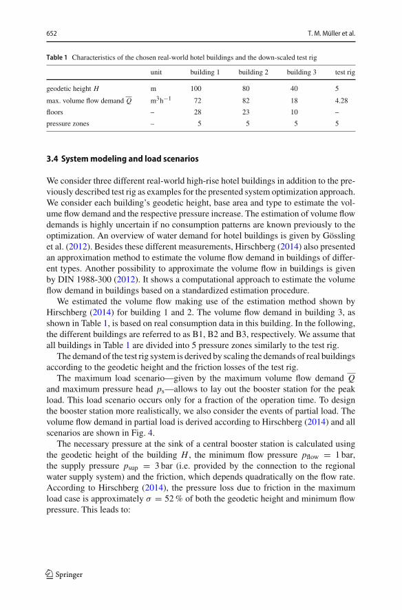
Table 1 Characteristics of the chosen real-world hotel buildings and the down-scaled test rig
unit building 1 building 2 building 3 test rig
geodetic height H m 100 80 40 5
max. volume flow demand Q m3h−1 72 82 18 4.28
floors – 28 23 10 –
pressure zones – 5 5 5 5
3.4 Systemmodeling and load scenarios
We consider three different real-world high-rise hotel buildings in addition to the pre-viously described test rig as examples for the presented system optimization approach.We consider each building’s geodetic height, base area and type to estimate the vol-ume flow demand and the respective pressure increase. The estimation of volume flowdemands is highly uncertain if no consumption patterns are known previously to theoptimization. An overview of water demand for hotel buildings is given by Gösslinget al. (2012). Besides these different measurements, Hirschberg (2014) also presentedan approximation method to estimate the volume flow demand in buildings of differ-ent types. Another possibility to approximate the volume flow in buildings is givenby DIN 1988-300 (2012). It shows a computational approach to estimate the volumeflow demand in buildings based on a standardized estimation procedure.
We estimated the volume flow making use of the estimation method shown byHirschberg (2014) for building 1 and 2. The volume flow demand in building 3, asshown in Table 1, is based on real consumption data in this building. In the following,the different buildings are referred to as B1, B2 and B3, respectively. We assume thatall buildings in Table 1 are divided into 5 pressure zones similarly to the test rig.
The demand of the test rig system is derived by scaling the demands of real buildingsaccording to the geodetic height and the friction losses of the test rig.
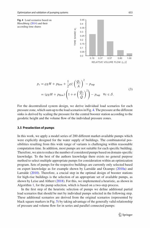
The maximum load scenario—given by the maximum volume flow demand Qand maximum pressure head ps—allows to lay out the booster station for the peakload. This load scenario occurs only for a fraction of the operation time. To designthe booster station more realistically, we also consider the events of partial load. Thevolume flow demand in partial load is derived according to Hirschberg (2014) and allscenarios are shown in Fig. 4.
The necessary pressure at the sink of a central booster station is calculated usingthe geodetic height of the building H , the minimum flow pressure pflow = 1 bar,the supply pressure psup = 3 bar (i.e. provided by the connection to the regionalwater supply system) and the friction, which depends quadratically on the flow rate.According to Hirschberg (2014), the pressure loss due to friction in the maximumload case is approximately σ = 52% of both the geodetic height and minimum flowpressure. This leads to:
123
Optimization and validation of pumping systems 653
Fig. 4 Load scenarios based onHirschberg (2014) and theiraccording time shares
ps = �gH + pflow + 1
2�ζ
(Qs
A
)2
− psup
= (�gH + pflow)
(1 + σ
(Qs
Q
)2)
− psup ∀s ∈ S.
(3)
For the decentralized system design, we derive individual load scenarios for eachpressure zone,which sumup to the load scenarios in Fig. 4. The pressure at the differentsinks is derived by scaling the pressure for the central booster station according to thegeodetic height and the volume flow of the individual pressure zones.
3.5 Preselection of pumps
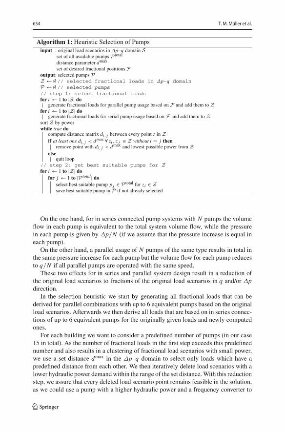
In this work, we apply a model series of 200 different market-available pumps whichwere explicitly designed for the water supply of buildings. The combinatorial pos-sibilities resulting from this wide range of variants is challenging within reasonablecomputation time. In addition, most pumps are not suitable for each specific building.Therefore,we aim to reduce the number of considered pumps based ondomain-specificknowledge. To the best of the authors knowledge there exists no general purposemethod to select multiple appropriate pumps for consideration within an optimizationprogram. Sets of pumps for the respective buildings are currently only selected basedon expert knowledge as for example shown by Larralde and Ocampo (2010a) andLarralde (2010). Therefore, a crucial step in the optimal design of booster stationsfor high-rise buildings is the selection of an appropriate set of available pumps, asshown by Leise and Altherr (2018). For this, we implemented a heuristic, as shown inAlgorithm 1, for the pump selection, which is based on a two-step process.
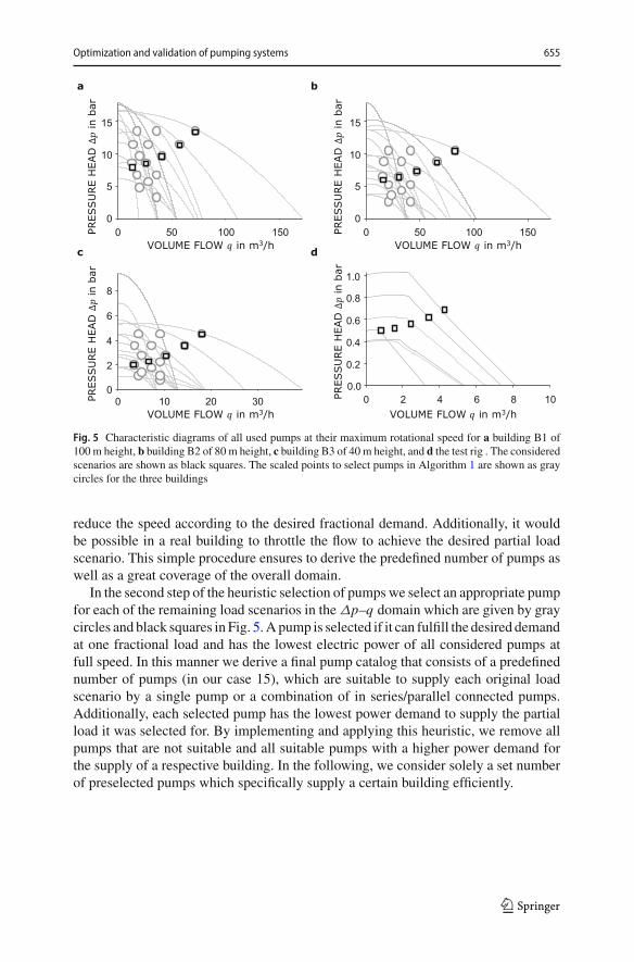
In the first step of the heuristic selection of pumps we define additional partialload scenarios that should be met by individual pumps selected in the following step.These additional scenarios are derived from the original scenarios (represented byblack square markers in Fig. 5) by taking advantage of the generally valid relationshipof pressure and volume flow for in series and parallel connected pumps:
123
654 T. M. Müller et al.
Algorithm 1: Heuristic Selection of Pumpsinput : original load scenarios in Δp–q domain S
set of all available pumps P total
distance parameter dmax
set of desired fractional positions Foutput: selected pumps PZ ← ∅ // selected fractional loads in Δp-q domainP ← ∅ // selected pumps// step 1: select fractional loadsfor i ← 1 to |S| do
generate fractional loads for parallel pump usage based on F and add them to Zfor i ← 1 to |Z| do
generate fractional loads for serial pump usage based on F and add them to Zsort Z by powerwhile true do
compute distance matrix di, j between every point z in Zif at least one di, j < dmax ∀ zi , z j ∈ Z without i = j then
remove point with di, j < dmax and lowest possible power from Zelse
quit loop// step 2: get best suitable pumps for Zfor i ← 1 to |Z| do
for j ← 1 to |P total| doselect best suitable pump p j ∈ P total for zi ∈ Zsave best suitable pump in P if not already selected
On the one hand, for in series connected pump systems with N pumps the volumeflow in each pump is equivalent to the total system volume flow, while the pressurein each pump is given by Δp/N (if we assume that the pressure increase is equal ineach pump).
On the other hand, a parallel usage of N pumps of the same type results in total inthe same pressure increase for each pump but the volume flow for each pump reducesto q/N if all parallel pumps are operated with the same speed.
These two effects for in series and parallel system design result in a reduction ofthe original load scenarios to fractions of the original load scenarios in q and/or Δpdirection.
In the selection heuristic we start by generating all fractional loads that can bederived for parallel combinations with up to 6 equivalent pumps based on the originalload scenarios. Afterwards we then derive all loads that are based on in series connec-tions of up to 6 equivalent pumps for the originally given loads and newly computedones.
For each building we want to consider a predefined number of pumps (in our case15 in total). As the number of fractional loads in the first step exceeds this predefinednumber and also results in a clustering of fractional load scenarios with small power,we use a set distance dmax in the Δp–q domain to select only loads which have apredefined distance from each other. We then iteratively delete load scenarios with alower hydraulic power demandwithin the range of the set distance.With this reductionstep, we assure that every deleted load scenario point remains feasible in the solution,as we could use a pump with a higher hydraulic power and a frequency converter to
123
Optimization and validation of pumping systems 655
0 2 4 6 8 10VOLUME FLOW in m3/h
PRES
SU
RE
HEA
D Δ
in b
ar
c d
b a
0 50 100 150VOLUME FLOW in m3/h
0
5
10
15
DAE
HE
RU
SSE
R PΔ
rabni
0 10 20 30VOLUME FLOW in m3/h
0
2
4
6
8
DAE
HE
RU
SSE
RPΔ
r abni
0 50 100 150VOLUME FLOW in m3/h
0
5
10
15
PRES
SU
RE
HEA
D Δ
in b
ar
0.0
0.2
0.4
0.6
0.8
1.0
Fig. 5 Characteristic diagrams of all used pumps at their maximum rotational speed for a building B1 of100 m height, b building B2 of 80 m height, c building B3 of 40 m height, and d the test rig . The consideredscenarios are shown as black squares. The scaled points to select pumps in Algorithm 1 are shown as graycircles for the three buildings
reduce the speed according to the desired fractional demand. Additionally, it wouldbe possible in a real building to throttle the flow to achieve the desired partial loadscenario. This simple procedure ensures to derive the predefined number of pumps aswell as a great coverage of the overall domain.
In the second step of the heuristic selection of pumps we select an appropriate pumpfor each of the remaining load scenarios in the Δp–q domain which are given by graycircles and black squares in Fig. 5.Apump is selected if it can fulfill the desired demandat one fractional load and has the lowest electric power of all considered pumps atfull speed. In this manner we derive a final pump catalog that consists of a predefinednumber of pumps (in our case 15), which are suitable to supply each original loadscenario by a single pump or a combination of in series/parallel connected pumps.Additionally, each selected pump has the lowest power demand to supply the partialload it was selected for. By implementing and applying this heuristic, we remove allpumps that are not suitable and all suitable pumps with a higher power demand forthe supply of a respective building. In the following, we consider solely a set numberof preselected pumps which specifically supply a certain building efficiently.
123

656 T. M. Müller et al.
4 Optimizationmodel
This section deals with the mathematical formulation of the previously introducedtechnical designproblem.The technical specifications aremodeled in a basic stochasticoptimization model (Sect. 4.1).
We reduce the two-stage stochastic problem to its Deterministic Equivalent Pro-gram by using multiple load scenarios. In our case, the first stage variables representinvestment and design decisions while second stage variables represent control deci-sions. Within this scenario based optimization approach binary variables are presentin both stages. Even in the second stage as the model takes into account that not allpumps are always switched on to meet the demand of the different load scenarios. Incontrast, some pumps may also be switched off and bypassed for efficiency reasons,especially in load cases with lower volume flow requirements.
Since pumps have nonlinear characteristics, the mixed-integer nonlinear program(MINLP) pumpmodel (Sect. 4.2) as well as two linear pumpmodels, allowing the for-mulation of a mixed-integer linear program (MILP), are presented. In a first approach,a piecewise linearized pump model (Sect. 4.3) is derived and in a second approach, apiecewise linear relaxed pump model (Sect. 4.4) is established.
4.1 Basic optimizationmodel
All derived optimization models in this contribution have a common mixed-integerlinear foundation, which we present in this section. The complete system design withall possibilities is modeled as a graph G = (V, E), in which the edges E model thepumps as well as the pipes. The junctions of the booster station are modeled as verticesV . The basic model’s variables, which are indicated by lower case letters, as well assets and parameters, indicated by upper case and Greek letters, are shown in Table 2.
The shared objective of all presented optimization models is the maximization ofthe net present value, cf. Meck et al. (2019). This results in a minimization of lifetimecost, which are approximated considering investment costs for pumps and frequencyconverters as well as discounted energy costs. The objective is shown in Obj. (5a). Weuse the annuity-present value factor APF to discount all costs to the present day.
We model an upper bound of pumps, Constr. (5b), to solely select a suitable subsetof all possible pumps in P in the final solution, i.e. maximum N buy pumps may bebought. The necessary precondition to use a pump is that it was bought, Constr. (5c).Purchased pumps should be used only in their physical domain. Therefore, we limit thepump speed, power and volume flow with Constr. (5d) and (5e). Constr. (5f) modelsthe volume flow conservation in the network, while Constr. (5g) models upper boundsfor the volume flow in each pipe.We demand the volume flow in the sinks to be exactlythe predefined volume flow for each scenario, as shown in Fig. 4 with Constr. (5h).It is imperative to choose at least one pump to connect the source with the sinks,Constr. (5i) and (5j). Constr. (5k)–(5m) prevent undesired topologies, as for exampleloops. The pressure at the inlet of a pump is set to the pressure at the source Psource
sin Constr. (5n) if a pump is connected to the source. The pressure increase from theinlet to the outlet of a pump is modeled by Constr. (5o). The pressure at the inlet and
123
Optimization and validation of pumping systems 657
Table 2 Decision variables, sets and parameters
Variable Domain Description
Δpi,s ; qi,s ; ni,s R+0 Pressure increase, volume flow and rotational speed of
pump i ∈ P in scenario s ∈ S
popumpi,s ; poFCi,s ; poi,s R
+0 Power consumption of pump i ∈ P , the associated
frequency converter and the sum of both in scenario s ∈ S
pini,s ; pouti,s R
+0 Pressure at inlet and outlet of pump i ∈ P , s ∈ S
qpipei, j,s R
+0 Volume flow between outlet of pump i ∈ P and inlet of
pump j ∈ P , s ∈ Sqsourcei,s R
+0 Volume flow between source and inlet of pump i ∈ P , s ∈ S
qsinki, f ,s R+0 Volume flow between outlet of pump i ∈ P and sink
f ∈ F , s ∈ SIndicator for connection between:
ti, j {0, 1} Outlet of pump i and inlet of pump j ,
tsourcei {0, 1} Source and inlet of pump i ,
tsinki, f {0, 1} Outlet of pump i and sink f ∈ Fxi,s {0, 1} Activation of pump i in scenario s ∈ S
yi ; yFCi {0, 1} Investment decision for pump i ∈ P and associated
frequency converter
Set Description
P Set of available pumps
S Set of demand scenarios with |S| = 5
F Set of sinks, which corresponds to individually suppliedpressure zones. For central systems applies |F | = 1, fordecentral systems |F | = 5
Parameter Range Description
APF R+0 Annuity-present value factor
Cpumpinvest,i R
+0 Investment costs of pump i ∈ P
CFCinvest,i R
+0 Investment costs of frequency converter for pump i ∈ P
Celect R+0 Electricity price (0.3 e/kWh)
Ws [0, 1] Time share of scenario s ∈ S.Ton R
+0 Total runtime per year (0.3 × 365d × 24h)
NbuyN Maximum number of pumps that can be purchased.
ΔPi ; P; Q;Poi ; Poi ; Ni , Ni R+0 Upper or lower bounds for the operating parameter of
pump i , i.e., pressure increase, pressure, volume flow,power, speed
Psources R
+0 Pressure at the source
Psinkf ,s ; Qbound
f ,s R+0 Pressure and volume flow demand at sink f ∈ F in
scenario s ∈ S
Pohydrs R
+0 Required hydraulic power s ∈ S
123

658 T. M. Müller et al.
Table 2 continued
Parameter Range Description
αi,m R+0 Pressure-volume flow regression coefficients for pump
i ∈ P with m ∈ {0, 1, 2}βi,m R
+0 Power-volume flow regression coefficients for pump i ∈ P
with m ∈ {0, 1, 2, 3}ζ inst. R
+0 Loss coefficient for the installation fittings of the pumps
ηpumpbest R
+0 Best efficiency of any pump in set P
ηFCi R+0 Efficiency of frequency converter of pump i ∈ P
outlet of an unused pump is set to zero, Constr. (5p). The pressure of a pump’s outletshould fulfill the predefined pressure requirements at the sink if it is connected to thesink, Constr. (5q). The pressure propagation between connected pumps is modeled byConstr. (5r). If a frequency converter for a certain pump is not purchased (yFCi = 0),the speed of the pump has to be set to the nominal speed (n = 1) in case of activity,Constr. (5s). If the pump is turned off, or a frequency converter is purchased, thisconstraint has to be deactivated, Constr. (5s). If a frequency converter is bought, thepump is speed controllable, but a part of the transmitted electrical power is dissipated,Constr. (5t). In addition, the electrical power for the pump motor is added to the totalpower, Constr. (5u). Moreover, we can say that the electrical power of the systemhas to be higher than the hydraulic power divided by the best efficiency of the bestpump, Constr. (5v). This provides a lower bound for the power consumption, whichsignificantly speeds up the optimization process, as shown by Müller et al. (2019a).
In the subsequently introduced models, we allow for the option to restrict the usageof in series connected pumps, as pumps connected in parallel correspond to the currentstandard installation procedure, cf. Sect. 3.2. A solely parallel connection can beachieved by adding the following constraint to the basic model (5):
ti, j = 0 ∀ i, j ∈ P. (4)
The objective as well as all so far presented constraints, Model (5) and Constr. (4),depend linearly on the decision variables. The accordingmixed-integer linear programdescribes the generic selection and usage of pumps to supply multiple sinks withrelevant connected pumps to derive a suitable booster station. Nevertheless, this modeldoes not contain the explicit modeling of the used pumps, as shown in Eq. (1) andEq. (2). Therefore, we present different methods to model these nonlinear relations oftype Δp = f (q, n) and po = g(q, n) in the following subsections.
min TonAPF Celect
∑
s∈SWs
∑
i∈Ppoi,s +
∑
i∈PCpumpinvest,i yi +
∑
i∈PCFCinvest,i y
FCi (5a)
subject to∑
i∈Pyi ≤ N buy (5b)
123
Optimization and validation of pumping systems 659
xi,s ≤ yi ∀i ∈ P, s ∈ S (5c)ni,s ≥ Ni xi,s ∀i ∈ P, s ∈ S (5d)
Δpi,s ≤ Pxi,s , qi,s ≤ Qxi,s , ni,s ≤ Ni xi,s ,
poi,s ≤ Poi , popumpi,s ≤ Poi xi,s ∀i ∈ P, s ∈ S (5e)
qi,s =∑
j∈Pqpipej,i,s + qsourcei,s =
∑
j∈Pqpipei, j,s +
∑
f ∈Fqsinki, f ,s ∀i ∈ P, s ∈ S (5f)
qpipei, j,s ≤ Q ti, j , qsourcei,s ≤ Q t sourcei , qsinki, f ,s ≤ Q t sinki, f ∀i, j ∈ P, f ∈ F , s ∈ S (5g)∑
i∈Pqsinki, f ,s = Qbound
f ,s ∀ f ∈ F , s ∈ S (5h)
∑
i∈Pt sinki, f ≥ 1 ∀ f ∈ F (5i)
∑
i∈Pt sourcei ≥ 1 (5j)
ti,i = 0 ∀i ∈ P (5k)∑
j∈Pti, j ≤ |P|(1 − t sourcei ) ∀i ∈ P (5l)
∑
j∈Pti, j ≤ |P|yi ,
∑
j∈Pt j,i ≤ |P|yi , t sourcei ≤ yi ,
∑
t∈Ft sinki, f ≤ yi ∀i ∈ P (5m)
pini,s − Psources
≤+≥− P(1 − t sourcei ) ∀i ∈ P, s ∈ S (5n)
pini,s + Δpi,s − pouti,s≤+≥− P(1 − xi,s) ∀i ∈ P, s ∈ S (5o)
pini,s ≤ P
⎛
⎝∑
j∈Pt j,i + t sourcei
⎞
⎠ , pouti,s ≤ P
⎛
⎝∑
j∈Pti, j +
∑
f ∈Ft sinki, f
⎞
⎠ ∀i ∈ P, s ∈ S (5p)
pouti,s − Psinkf ,s
≤+≥− P(1 − t sinki, f ) ∀i ∈ P, f ∈ F , s ∈ S (5q)
pouti,s − pinj,s≤+≥− P(1 − ti, j ) ∀i, j ∈ P, s ∈ S (5r)
ni,s − 1 ≤+≥−((1 − xi,s) + yFCi
)∀i ∈ P, s ∈ S, (5s)
(1 − ηFCi
)poi,s − poFCi,s ≤ Poi
(1 − yFCi
)∀i ∈ P, s ∈ S (5t)
poi,s = popumpi,s + poFCi,s ∀i ∈ P, s ∈ S (5u)
∑
i∈Ppoi,s ≥ Pohydrs /η
pumpbest ∀s ∈ S (5v)
4.2 Mixed-integer nonlinear pumpmodel
The most accurate modeling approach is given by a nonlinear approach in whicheach considered pump is modeled with nonlinear constraints according to Eq. (1) andEq. (2). We add all pumps by adding
Δpi,s = (αi,0 − ζ inst.) qi,s2 +
2∑
m=1
αi,m qi,s2−m ni,s
m ∀i ∈ P, s ∈ S, (6a)
123
660 T. M. Müller et al.
Table 3 Additional variables, sets and parameters for PWL
Variable Domain Description
λu,v,i,s [0, 1] Additional variable to model the piecewise linearapproximation based on grid point (u, v) and pumpi ∈ P in scenario s ∈ S
ai,s,k {0, 1} Binary variable to select simplex k ∈ K for pump i ∈ Pin scenario s ∈ S
Set Description
Q Set of grid points in direction of the volume flow q
N Set of grid points in direction of the speed n
K Set of simplices
K(u, v, i, s) Subset of simplices which contain grid point (u, v) forpump i ∈ P in scenario s ∈ S
Parameter Range Description
Qu,v,i Grid values in q direction for pump i ∈ PNu,v,i Grid values in n direction for pump i ∈ PΔPu,v,i Pressure value at grid point (Qu,v,i , Nu,v,i ) by
evaluating Eq. 1 for pump i ∈ PPo
pumpu,v,i Power value at grid point (Qu,v,i , Nu,v,i ) by evaluating
Eq. 2 for pump i ∈ P
popumpi,s =
3∑
m=0
βi,m qi,s3−m ni,s
m ∀i ∈ P, s ∈ S, (6b)
to the basic model in Eq. (5), where ζ inst. is the pressure loss factor of the fittingsused for installing the pump into the system. The benefits of this approach are a fastimplementation and a highly accurate model, while the drawbacks are potentially highsolution times.
4.3 Piecewise linearized pumpmodel
A common approach to solve nonlinear non-convex optimization models with integervariables, is to make use of approximations based on piecewise linearization (PWL)techniques, cf. Geißler et al. (2012). Linearization of all nonlinear constraints results ina mixed-integer linear program, which can then be solved by state-of-the-art solversas for example GUROBI (GUROBI 2020) or CPLEX (IBM 2020). Piecewise lin-earization methods are therefore applied in a high variety of applications, both withinclassical operations research, as well as technical applications, e.g. Misener et al.(2009), Morsi et al. (2012), Rausch et al. (2016) and Mikolajková et al. (2018). Theunderlying modeling to reformulate a nonlinear functional relationship as linear con-straints can be implemented by multiple methods, as shown by Misener and Floudas(2010), Vielma et al. (2010) and Geißler et al. (2012).
123

Optimization and validation of pumping systems 661
In this contribution, we use the convex combinationmethod, as described byVielmaet al. (2010), to model the nonlinear relations of the pressure head Δp = f (q, n) andof the power po = g(q, n) as piecewise linearized function approximations. Alladditional variables, sets and parameters for the PWL are shown in Table 3. Insteadof using Eq. (6) to model the nonlinear pump characteristics, we model a piecewiselinearized approximation by using the set of constraints (7).
qi,s −∑
u∈Q
∑
v∈Nλu,v,i,s Qu,v,i
≤+≥− (1 − xi,s)Q ∀i ∈ P, s ∈ S, (7a)
ni,s −∑
u∈Q
∑
v∈Nλu,v,i,s Nu,v,i
≤+≥− (1 − xi,s)Ni ∀i ∈ P, s ∈ S, (7b)
Δpi,s −∑
u∈Q
∑
v∈Nλu,v,i,sΔPu,v,i
≤+≥− (1 − xi,s)P ∀i ∈ P, s ∈ S, (7c)
popumpi,s −
∑
u∈Q
∑
v∈Nλu,v,i,s Po
pumpu,v,i
≤+≥− (1 − xi,s)Poi ∀i ∈ P, s ∈ S, (7d)
∑
u∈Q
∑
v∈Nλu,v,i,s = 1 ∀i ∈ P, s ∈ S, (7e)
∑
k∈Kai,s,k = 1 ∀i ∈ P, s ∈ S, (7f)
λu,v,i,s −∑
k∈K(u,v,i,s)
ai,s,k ≤ 0 ∀u ∈ Q, v ∈ N , i ∈ P, s ∈ S. (7g)
The index sets Q and N represent grid points in the (q, n) domain in which thepressure ΔPu,v,i,s and power Popump
u,v,i,s are evaluated for each pump i ∈ P beforeoptimization according to Eqs. (1) and (2). The pressure losses and additional powerfor frequency converters are added to these values in the preprocessing of the opti-mization to derive an equivalent description, as shown in Constr. (6). Besides thesegrid points, we have to use additional binary variables ai,s,k ∈ {0, 1} and continuousvariables λu,v,i,s ∈ [0, 1] to ensure a piecewise linearized approximation. The set Kin Constr. (7f) contains all segments of the piecewise linearized approximation. Inturn, the subset K(u, v, i, s) in Constr. (7g) covers all segments that contain the gridpoint (u, v) for pump i and scenario s. These additional constraints are added to theoptimization program in model (5), which results in a mixed-integer linear programthat can be solved by common MILP solvers.
4.4 Piecewise linear relaxed pumpmodel
As a third possibility we use piecewise linear relaxed pump models within the finaloptimization program. Relaxations are often used in the MINLP solution process,as shown by Puranik and Sahinidis (2017), to derive valid lower bounds. A generalintroduction to relaxation methods for nonlinear network design problems is given byHumpola and Fügenschuh (2015). Relaxation methods with piecewise linear underes-
123
662 T. M. Müller et al.
0 10 20 30 40 50VOLUME FLOW in m³/h
00.40.60.81
ROTATIONAL SPEED
0
DAE
HE
RU
SSE
RPΔ
rabn i
1
2
3
4
5
6
PRES
SU
RE
HEA
D Δ
in b
ar
a b
1
2
3
4
5
6
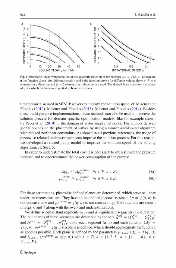
Fig. 6 Piecewise linear overestimation of the quadratic function of the pressure Δp = f (q, n). Shown area the function Δp(q) for different speeds n and b the function Δp(n) for different volume flows q. R = 6elements in q direction and K = 2 elements in n direction are used. The dashed lines in a show the valuesof q for which the lines were plotted in b and vice versa
timators are also used inMINLP solvers to improve the solution speed, cf.Misener andFloudas (2012), Misener and Floudas (2013), Misener and Floudas (2014). Besidesthese multi-purpose implementations, these methods can also be used to improve thesolution process for domain specific optimization models, like for example shownby Pecci et al. (2019) in the domain of water supply networks. The authors derivedglobal bounds on the placement of valves by using a Branch-and-Bound algorithmwith relaxed nonlinear constraints. As shown in all previous references, the usage ofpiecewise relaxed underestimators can improve the solution process. For this reason,we developed a relaxed pump model to improve the solution speed of the solvingalgorithm, cf. Sect. 5.
In order to underestimate the total cost it is necessary to overestimate the pressureincrease and to underestimate the power consumption of the pumps:
Δpi,s ≤ Δprelaxedi,s ∀i ∈ P, s ∈ S, (8a)
popumpi,s ≥ porelaxedi,s ∀i ∈ P, s ∈ S. (8b)
For these estimations, piecewise defined planes are determined, which serve as linearunder- or overestimators. They have to be defined piecewise, since Δp = f (q, n) isnot concave in n and popump = g(q, n) is not convex in q. The functions are shownin Figs. 6 and 7 along with the over- and underestimations.
We define R equidistant segments in q- and K equidistant segments in n direction.The boundaries of these segments are described by the setsQseg = {Qseg
1 , ..., Qseg1+R}
and N seg = {N seg1 , ..., N seg
1+K }. For each segment (u, v) and each function (Δp =f (q, n), popump = g(q, n)) a plane is defined, which should approximate the functionas good as possible. Each plane is defined by the parameters γi,k,u,v (Δp = f (q, n))and δi,k,u,v (popump = g(q, n)) with i ∈ P , k ∈ {1, 2, 3}, u ∈ {1, ...., R} , v ∈{1, ..., K }.
123
Optimization and validation of pumping systems 663
0.40.60.810
0 10 20 30 40 50
1
2
3
4
5
0
1
2
3
4
5
VOLUME FLOW in m³/h ROTATIONAL SPEED
REW
OPin
kW
POW
ER
in k
WPO
WER
in
kW
REW
OPin
kW
a b
c d
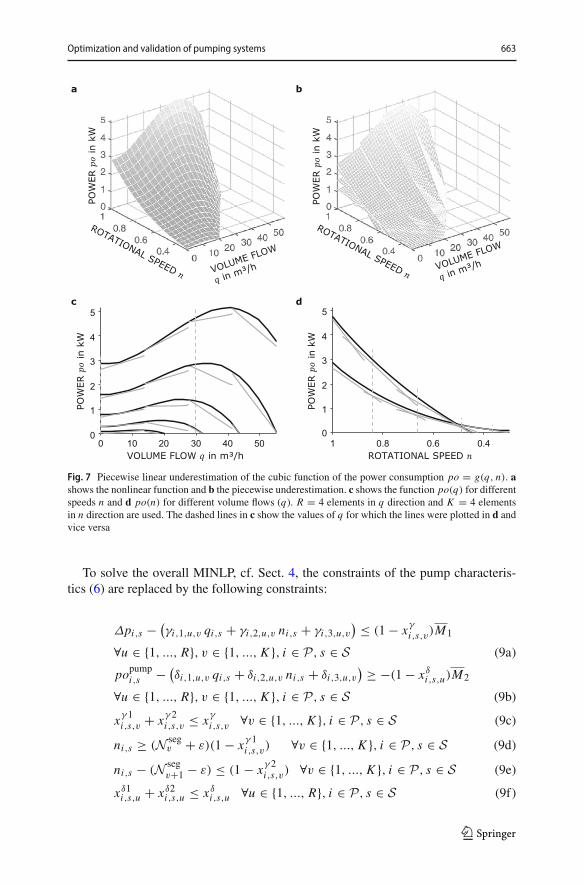
Fig. 7 Piecewise linear underestimation of the cubic function of the power consumption po = g(q, n). ashows the nonlinear function and b the piecewise underestimation. c shows the function po(q) for differentspeeds n and d po(n) for different volume flows (q). R = 4 elements in q direction and K = 4 elementsin n direction are used. The dashed lines in c show the values of q for which the lines were plotted in d andvice versa
To solve the overall MINLP, cf. Sect. 4, the constraints of the pump characteris-tics (6) are replaced by the following constraints:
Δpi,s − (γi,1,u,v qi,s + γi,2,u,v ni,s + γi,3,u,v
) ≤ (1 − xγ
i,s,v)M1
∀u ∈ {1, ..., R}, v ∈ {1, ..., K }, i ∈ P, s ∈ S (9a)
popumpi,s − (
δi,1,u,v qi,s + δi,2,u,v ni,s + δi,3,u,v
) ≥ −(1 − xδi,s,u)M2
∀u ∈ {1, ..., R}, v ∈ {1, ..., K }, i ∈ P, s ∈ S (9b)
xγ 1i,s,v + xγ 2
i,s,v ≤ xγ
i,s,v ∀v ∈ {1, ..., K }, i ∈ P, s ∈ S (9c)
ni,s ≥ (N segv + ε)(1 − xγ 1
i,s,v) ∀v ∈ {1, ..., K }, i ∈ P, s ∈ S (9d)
ni,s − (N segv+1 − ε) ≤ (1 − xγ 2
i,s,v) ∀v ∈ {1, ..., K }, i ∈ P, s ∈ S (9e)
xδ1i,s,u + xδ2
i,s,u ≤ xδi,s,u ∀u ∈ {1, ..., R}, i ∈ P, s ∈ S (9f)
123
664 T. M. Müller et al.
qi,s ≥ (Qsegu + ε)(1 − xδ1
i,s,u) ∀u ∈ {1, ..., R}, i ∈ P, s ∈ S (9g)
qi,s − (Qsegu+1 − ε) ≤ Q(1 − xδ2
i,s,u) ∀u ∈ {1, ..., R}, i ∈ P, s ∈ S (9h)
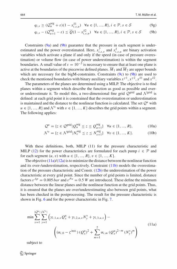
Constraints (9a) and (9b) guarantee that the pressure in each segment is under-estimated and the power overestimated. Here, xγ
i,s,v and xδi,s,u are binary activation
variables which activate a plane if and only if the speed (in case of pressure overes-timation) or volume flow (in case of power underestimation) is within the segmentboundaries. A small value of ε = 10−3 is necessary to ensure that at least one plane isactive at the boundaries of the piecewise defined planes. M1 and M2 are upper boundswhich are necessary for the bigM-constraints. Constraints (9c) to (9h) are used tocheck the mentioned boundaries with binary auxiliary variables xγ 1, xγ 2, xδ1 and xδ2.
The parameters of the planes are determined using a MILP. The objective is to findplanes within a segment which describe the function as good as possible and over-or underestimate it. To model this, a two-dimensional fine grid Qgrid and N grid isdefined: at each grid point it is constrained that the overestimation or underestimationis maintained and the distance to the nonlinear function is calculated. The setQu withu ∈ {1, ..., R} andN v with v ∈ {1, ..., K } describes the grid points within a segment.The following applies:
Qu = {z ∈ Qgrid|Qsegu ≤ z ≤ Qseg
u+1} ∀u ∈ {1, ..., R}, (10a)
N v = {z ∈ N grid|N segv ≤ z ≤ N seg
v+1} ∀v ∈ {1, ..., K }. (10b)
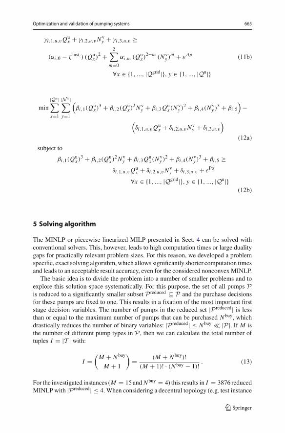
With these definitions, both, MILP (11) for the pressure characteristic andMILP (12) for the power characteristics are formulated for each pump i ∈ P andfor each segment (u, v) with u ∈ {1, ..., R}, v ∈ {1, ..., K }.
The objective (11a)/(12a) is tominimize the distance between the nonlinear functionand its over-/underestimation, respectively. Constraint (11b) models the overestima-tion of the pressure characteristic and Constr. (12b) the underestimation of the powercharacteristic at every grid point. Since the number of grid points is limited, distancefactors εΔp = 0.005 bar and εPo = 0.5W are introduced. These define the minimumdistance between the linear planes and the nonlinear function at the grid points. Thus,it is ensured that the planes are over/underestimating also between grid points, whathas been checked in the postprocessing. The result for the pressure characteristic isshown in Fig. 6 and for the power characteristic in Fig. 7.
min|Qu |∑
x=1
|N v |∑
y=1
(γi,1,u,vQ
ux + γi,2,u,vN
vy + γi,3,u,v
)−
((αi,0 − ζ inst.) (Qu
x )2 +
2∑
m=1
αi,m (Qux )
2−m(N v
y )m
) (11a)
subject to
123
Optimization and validation of pumping systems 665
γi,1,u,vQux + γi,2,u,vN
vy + γi,3,u,v ≥
(αi,0 − ζ inst.) (Qux )
2 +2∑
m=0
αi,m (Qux )
2−m(N v
y )m + εΔp
∀x ∈ {1, ..., |Qgrid|}, y ∈ {1, ..., |Qu|}
(11b)
min|Qu |∑
x=1
|N v |∑
y=1
(βi,1(Q
ux )
3 + βi,2(Qux )
2N vy + βi,3Q
ux (N
vy )
2 + βi,4(Nvy )
3 + βi,5
)−
(δi,1,u,vQ
ux + δi,2,u,vN
vy + δi,3,u,v
)
(12a)
subject to
βi,1(Qux )
3 + βi,2(Qux )
2N vy + βi,3Q
ux (N
vy )
2 + βi,4(Nvy )
3 + βi,5 ≥δi,1,u,vQ
ux + δi,2,u,vN
vy + δi,3,u,v + εPo
∀x ∈ {1, ..., |Qgrid|}, y ∈ {1, ..., |Qu|}(12b)
5 Solving algorithm
The MINLP or piecewise linearized MILP presented in Sect. 4 can be solved withconventional solvers. This, however, leads to high computation times or large dualitygaps for practically relevant problem sizes. For this reason, we developed a problemspecific, exact solving algorithm,which allows significantly shorter computation timesand leads to an acceptable result accuracy, even for the considered nonconvexMINLP.
The basic idea is to divide the problem into a number of smaller problems and toexplore this solution space systematically. For this purpose, the set of all pumps Pis reduced to a significantly smaller subset P reduced ⊆ P and the purchase decisionsfor these pumps are fixed to one. This results in a fixation of the most important firststage decision variables. The number of pumps in the reduced set |P reduced| is lessthan or equal to the maximum number of pumps that can be purchased N buy, whichdrastically reduces the number of binary variables: |P reduced| ≤ N buy |P|. If M isthe number of different pump types in P , then we can calculate the total number oftuples I = |T | with:
I =(M + N buy
M + 1
)= (M + N buy)!
(M + 1)! · (N buy − 1)! . (13)
For the investigated instances (M = 15 and N buy = 4) this results in I = 3876 reducedMINLPwith |P reduced| ≤ 4.When considering a decentral topology (e.g. test instance
123

666 T. M. Müller et al.
Algorithm 2: Generic description of the solving algorithm.input : set of pumps P ; load scenarios; instance-specific parametersoutput: best topology and control; solution information
// preprocessinginitialize all possible feasible purchase decisions TI = {1, 2, . . . , I }L = {L1, L2, . . . , L I }U = {U1,U2, . . . ,UI }U ← Uj = ∞∀ j ∈ IL ← L j = ∑
s∈S Ws Pohydrs ∀ j ∈ I
Uglobal = ∞, Lglobal = min(L)
// main part
while Uglobal > Lglobal do// heuristic for upper-bound-search
estimate primal bound for each tuple, U estj ∀ j ∈ I
solve reduced MINLP for the most promising tuple (lowest U estj )
if infeasible or dual bound > Uglobal thenremove tuple
elseupdate tuple information in: U ,L
update global information: Uglobal = min(U), Lglobal = min(L)// lower-bound-searchsolve reduced MINLP or relaxed, reduced MILP for tuple with lowest dual bound in Lif infeasible or dual bound > Uglobal then
remove tupleelse
update tuple information in: U (only if MINLP was solved), Lupdate global information: Uglobal = min(U), Lglobal = min(L)
B1.D, cf. 6.1) this yields aMINLPwith 425 variables (64 binary) and 1057 constraints(41 nonlinear). In contrast to this is a singleMINLPwith |P| = M×N buy = 60 pumps.This yields 26581 variables (4380 binary) and 82562 constraints (601 nonlinear). Theresulting reduced MINLP is therefore less challenging in terms of combinatorics andcan generally be solved faster. The goal is to efficiently explore the set of possiblepurchase decisions T , given the reduced set of available pumps, while also cutting offnon-optimal solutions.
The solving algorithm is shown in Algorithm 2. For better clarity, we define theindex set I = {1, 2, . . . , I } based on Eq. (13). First, the set of pump-tuples Tis created and physically inadmissible tuples are removed during preprocessing. Inaddition, a set of lower bounds L = {L1, L2, . . . , L I } for the energy costs of eachtuple Tj ∈ T is analytically calculated based on domain-specific knowledge. Besides,a set of all primal upper bounds U = {U1,U2, . . . ,UI } is defined and each part isset to ∞ before optimization. For the considered overall minimization problem, theprimal bound is the minimal primal solution of a tuple U global = min(U) (best foundsolution), which is infinite at the start. The dual bound of the overall minimizationproblem Lglobal should be raised. Therefore, the weakest dual bound in one of thesubproblems/tuples is determined. Thus, the dual bound of the overall problem is
123

Optimization and validation of pumping systems 667
bounded by the lowest dual bound of a tuple Lglobal ≥ min(L). It is initialized usingthe preprocessed bounds for the energy and the known investment costs of the pumps.Now the search for better primal and dual solutions is repeated until the overall problemhas been solved to proven global optimality. The global primal and dual bounds areupdated in each step and proven weak solutions or infeasible solutions are cut off. Inthe following, the single steps of the solving algorithm are explained in detail.
5.1 Preprocessing
First, the set of purchase decisions Tj ∈ T ∀ j ∈ I is generated, each consisting of areduced set of pumpsP reduced
j ⊆ P with j ∈ I. For each tuple Tj ∈ T , it is determined
whether the pumps of the tuple P reducedj can fulfill the required load demand. There
are three elimination criteria:
(i) The sum of the maximum pressure head of all pumps is smaller than required.Even a series connection of all pumps could not provide the required pressure.
(ii) The sum of the maximum volume flow of all pumps is smaller than required.Even a parallel connection of all pumps could not provide the required volumeflow.
(iii) The sum of the maximum hydraulic power of all pumps is smaller than required.Even if all pumps would be operated at the point of maximum hydraulic power,it would not be sufficient.
Tuples that comply with any of these criteria are deleted immediately. This canefficiently reduce the number of tuples. Nevertheless, this excludes only a subset ofall infeasible solutions.
The minimum cost are underestimated for each of the remaining tuples. Since thepurchase decision for a certain pump set is fixed, the investment costs of this pumpset can be calculated directly. The purchase decision for frequency converters is setto zero. We underestimate the power consumption and thus the energy cost. For eachTj ∈ T the underestimated power consumption Polb,physs, j is calculated by the hydraulic
power Pohydrs and best efficiency of any pump in the tuple ηpumpbest, j in every scenario
s ∈ S. For each tuple j ∈ I the following underestimation is valid:
∑
s∈SWs
∑
i∈Ppoi,s ≥
∑
s∈SWs Po
lb,physs, j =
∑
s∈SWs Po
hydrs /η
pumpbest,j . (14)
This corresponds to the hypothetical case that the pump with the highest efficiencyprovides the required hydraulic power in its best-efficiency point all by itself. Theresulting cost according to Obj. (5a) underestimates the true cost and is thus a lowerbound,which is based on physical principles. This consideration allows to cut offmanytuples early. The power dissipated in the frequency converter is usually one order ofmagnitude smaller than the electrical power in the motor and is therefore neglected inthis estimation.
Finally, the global primal and dual bounds are initialized in preprocessing. Theglobal primal bound is the value of the best valid solution and is initially set to infinity.
123

668 T. M. Müller et al.
The global dual bound equals the minimum value of the lower bound of any tuple. Itis initialized to the minimum of the values estimated by Eq. (14).
5.2 Bound improvement
After preprocessing, the gap between the primal and dual bound is attempted to bereduced over time. On the one hand, better primal solutions are searched for. On theother hand, the minimum values of the lower bound of the tuples are improved toincrease the dual bound of the overall minimization problem. If the resulting value ofthe lower bound of a tuple is above the global primal bound, it can be cut off.
5.2.1 Upper bound search
In order to find a new, better primal solution, the objective value of each tuple Tj ∈ Tis estimated in each step. The exact MINLP is then solved for the tuple with the bestestimated objective value, i.e. the most promising set of pumps.Estimation of the Objective Value The value of the primal solution of a tuple Tj ∈ Tis estimated using a heuristic. It is assumed that the difference between the lowerbound of the power consumption estimated during preprocessing Polb,physs, j , Eq. (14),
and the power consumptions’ exact value of the primal solution of a tuple Poprimals, j is
comparable for all tuples j ∈ I. We calculate this difference for all tuples in T forwhich we already know the primal solution by:
vs, j = (Poprimals, j − Polb,physs, j )/Polb,physs, j ∀s ∈ S, j ∈ I. (15)
The expected power consumption Poexps,j of tuples for which we have not yet com-puted a primal solution is estimated using the mean of the deviation vs, j of all tupleswith known primal solution:
∑
s∈SWs
∑
i∈Ppoi,s ≈
∑
s∈SWs Po
exps, j
=∑
s∈SWs
(1 +
∑m∈Iprimal vs,m
|Iprimal|)Polb,physs, j ∀ j ∈ I ,
(16)
where Iprimal = { j ∈ I | ∃Uj < ∞} is the index set of tuples with finite primalsolution. Based on this, the total cost is estimated according to Obj. (5a). Here, theexact known investment costs of the pumps are considered while the costs for thefrequency converters are neglected.Search for Better Primal SolutionWhen searching for a new primal solution, the tuplewith the lowest expected cost is selected. The set of pumps is reduced to the purchasedpumps P reduced
j in the selected tuple Tj . The MINLP from Sect. 4 is formulated withthe reduced set of pumps and the purchase decision variables are set to yi = 1 ∀ i ∈{1, ..., |P reduced
j |}.
123
Optimization and validation of pumping systems 669
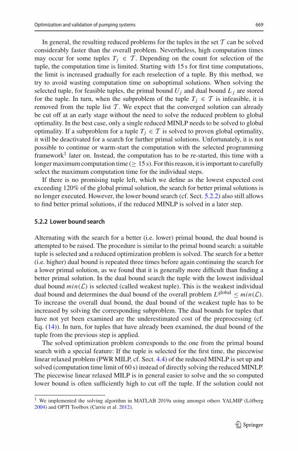
In general, the resulting reduced problems for the tuples in the set T can be solvedconsiderably faster than the overall problem. Nevertheless, high computation timesmay occur for some tuples Tj ∈ T . Depending on the count for selection of thetuple, the computation time is limited. Starting with 15s for first time computations,the limit is increased gradually for each reselection of a tuple. By this method, wetry to avoid wasting computation time on suboptimal solutions. When solving theselected tuple, for feasible tuples, the primal bound Uj and dual bound L j are storedfor the tuple. In turn, when the subproblem of the tuple Tj ∈ T is infeasible, it isremoved from the tuple list T . We expect that the converged solution can alreadybe cut off at an early stage without the need to solve the reduced problem to globaloptimality. In the best case, only a single reduced MINLP needs to be solved to globaloptimality. If a subproblem for a tuple Tj ∈ T is solved to proven global optimality,it will be deactivated for a search for further primal solutions. Unfortunately, it is notpossible to continue or warm-start the computation with the selected programmingframework1 later on. Instead, the computation has to be re-started, this time with alongermaximumcomputation time (≥ 15 s). For this reason, it is important to carefullyselect the maximum computation time for the individual steps.
If there is no promising tuple left, which we define as the lowest expected costexceeding 120% of the global primal solution, the search for better primal solutions isno longer executed. However, the lower bound search (cf. Sect. 5.2.2) also still allowsto find better primal solutions, if the reduced MINLP is solved in a later step.
5.2.2 Lower bound search
Alternating with the search for a better (i.e. lower) primal bound, the dual bound isattempted to be raised. The procedure is similar to the primal bound search: a suitabletuple is selected and a reduced optimization problem is solved. The search for a better(i.e. higher) dual bound is repeated three times before again continuing the search fora lower primal solution, as we found that it is generally more difficult than finding abetter primal solution. In the dual bound search the tuple with the lowest individualdual bound min(L) is selected (called weakest tuple). This is the weakest individualdual bound and determines the dual bound of the overall problem Lglobal ≤ min(L).To increase the overall dual bound, the dual bound of the weakest tuple has to beincreased by solving the corresponding subproblem. The dual bounds for tuples thathave not yet been examined are the underestimated cost of the preprocessing (cf.Eq. (14)). In turn, for tuples that have already been examined, the dual bound of thetuple from the previous step is applied.
The solved optimization problem corresponds to the one from the primal boundsearch with a special feature: If the tuple is selected for the first time, the piecewiselinear relaxed problem (PWRMILP, cf. Sect. 4.4) of the reduced MINLP is set up andsolved (computation time limit of 60 s) instead of directly solving the reducedMINLP.The piecewise linear relaxed MILP is in general easier to solve and the so computedlower bound is often sufficiently high to cut off the tuple. If the solution could not
1 We implemented the solving algorithm in MATLAB 2019a using amongst others YALMIP (Löfberg2004) and OPTI Toolbox (Currie et al. 2012).
123

670 T. M. Müller et al.
be cut off, the tuple is re-selected at a subsequent loop iteration and then the reducedMINLP is solved, whereby the initial computation time is again limited to 15 s andsubsequently increased in later iterations.
5.2.3 Parallelization
To further reduce computation times, the presented solving algorithm is parallelized.In each step N optimization problems are solved simultaneously on different cores:Therefore, not only a single tuplewith the best expected primal bound (in case of primalsearch) or lowest dual bound (in case of dual search) is selected, but N tuples withthe best expected primal or lowest dual bounds are solved. If a tuple is solved beforefinishing the computation of any of the other first N tuples, the next best/weakest tupleis solved on the available core. The results of the computed tuples are synchronizedafter the computation of the first N tuples is finished.
6 Computational results
In this section the results of the optimization problems are discussed. First, the setof test instances, which are scenarios of high technological importance, are presentedand the implementation and settings are clarified. Based on this, the performance ofthe different solving approaches is presented. Afterwards, a technical discussion ofthe results and the significance for practice are given.
6.1 Selection of test instances
The previously presented different systems (Sect. 3) and the wide range of variationsare analyzed carefully to choose technologically meaningful test instances. Testedinstances are numerated in Table 4, in which the different possible physical variantsare listed. For each of the buildings B1–B3 and the test rig three different topologies areconsidered. (i) Parallel connection of the pumps for a central booster station (|F | = 1,Constr. (4) active), hereinafter referred to as parallel. (ii) Unrestricted topology fora central booster station (|F | = 1, Constr. (4) not active), hereinafter referred to ascentral. (iii) Unrestricted topology for a decentral booster station (|F | = 5, Constr. (4)not active), hereinafter referred to as decentral. The complexity increases significantlyin the order of the listed topologies due to their increasing degrees of freedom. Theheuristic presented in Sect. 3.5 is used to select 15 different pump types for each ofthe buildings B1–B3. Each pump type is available N avail = 4 times which leads toa total set of |P| = 15 × 4 = 60 pumps. In total, up to N buy = 4 pumps can bepurchased and installed per booster station. For the test rig the set of pumps is limitedto the |P| = 13 available pumps (6 different types), where up to N buy = 6 can bepurchased and installed. While for the buildings B1–B3 a frequency converter has tobe installed additionally to allow for speed control, all considered pumps for the testrig are already equipped with frequency converters and therefore the decision to buya frequency converter is disregarded. The characteristic curves as well as costs of the
123
Optimization and validation of pumping systems 671
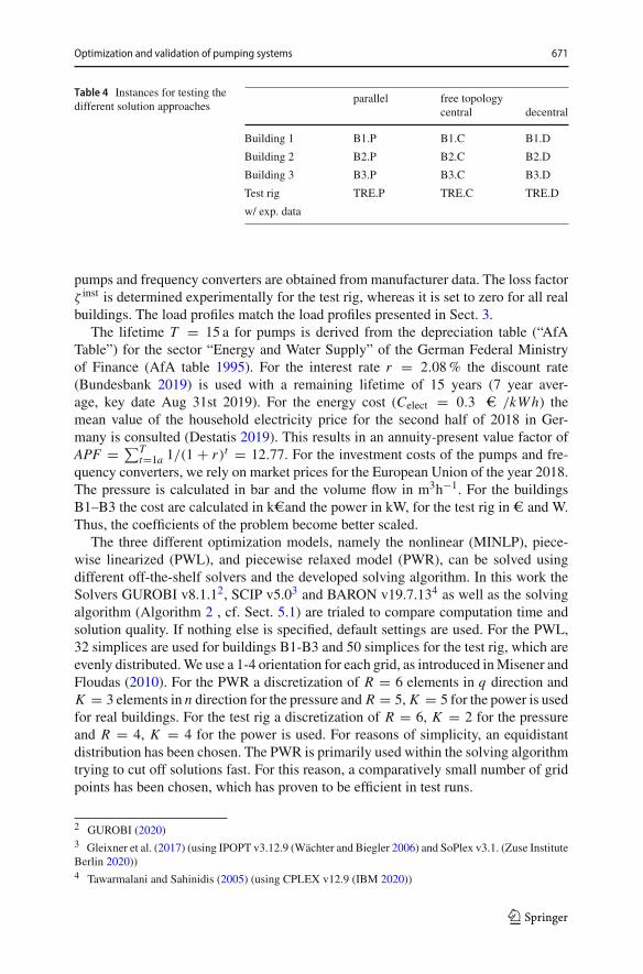
Table 4 Instances for testing thedifferent solution approaches
parallel free topologycentral decentral
Building 1 B1.P B1.C B1.D
Building 2 B2.P B2.C B2.D
Building 3 B3.P B3.C B3.D
Test rig TRE.P TRE.C TRE.D
w/ exp. data
pumps and frequency converters are obtained from manufacturer data. The loss factorζ inst is determined experimentally for the test rig, whereas it is set to zero for all realbuildings. The load profiles match the load profiles presented in Sect. 3.
The lifetime T = 15 a for pumps is derived from the depreciation table (“AfATable”) for the sector “Energy and Water Supply” of the German Federal Ministryof Finance (AfA table 1995). For the interest rate r = 2.08% the discount rate(Bundesbank 2019) is used with a remaining lifetime of 15 years (7 year aver-age, key date Aug 31st 2019). For the energy cost (Celect = 0.3 e /kWh) themean value of the household electricity price for the second half of 2018 in Ger-many is consulted (Destatis 2019). This results in an annuity-present value factor ofAPF = ∑T
t=1a 1/(1 + r)t = 12.77. For the investment costs of the pumps and fre-quency converters, we rely on market prices for the European Union of the year 2018.The pressure is calculated in bar and the volume flow in m3h−1. For the buildingsB1–B3 the cost are calculated in keand the power in kW, for the test rig in e and W.Thus, the coefficients of the problem become better scaled.
The three different optimization models, namely the nonlinear (MINLP), piece-wise linearized (PWL), and piecewise relaxed model (PWR), can be solved usingdifferent off-the-shelf solvers and the developed solving algorithm. In this work theSolvers GUROBI v8.1.12, SCIP v5.03 and BARON v19.7.134 as well as the solvingalgorithm (Algorithm 2 , cf. Sect. 5.1) are trialed to compare computation time andsolution quality. If nothing else is specified, default settings are used. For the PWL,32 simplices are used for buildings B1-B3 and 50 simplices for the test rig, which areevenly distributed.We use a 1-4 orientation for each grid, as introduced inMisener andFloudas (2010). For the PWR a discretization of R = 6 elements in q direction andK = 3 elements in n direction for the pressure and R = 5, K = 5 for the power is usedfor real buildings. For the test rig a discretization of R = 6, K = 2 for the pressureand R = 4, K = 4 for the power is used. For reasons of simplicity, an equidistantdistribution has been chosen. The PWR is primarily used within the solving algorithmtrying to cut off solutions fast. For this reason, a comparatively small number of gridpoints has been chosen, which has proven to be efficient in test runs.
2 GUROBI (2020)3 Gleixner et al. (2017) (using IPOPT v3.12.9 (Wächter and Biegler 2006) and SoPlex v3.1. (Zuse InstituteBerlin 2020))4 Tawarmalani and Sahinidis (2005) (using CPLEX v12.9 (IBM 2020))
123
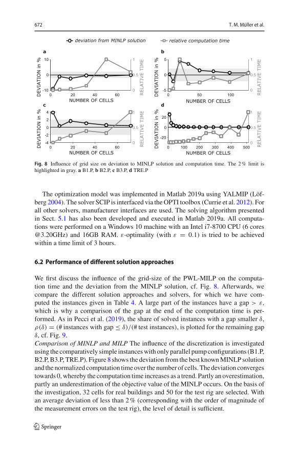
672 T. M. Müller et al.
0 20 40 60NUMBER OF CELLS
-10
0
10
0
0.5
1
0 50 100-5
0
5
0
0.5
1
0 20 40 60-4
-2
0
2
4
0
0.5
1
0 100 200 300 400 500
-20
0
20
0
0.5
1
%ni
NO IT
A IVE
D REL
ATI
VE
TIM
E
relative computation timedeviation from MINLP solution
NUMBER OF CELLS
%ni
NOIT
AIVE
D REL
ATI
VE
TIM
E
NUMBER OF CELLSD
EVIA
TIO
N in
%
REL
ATI
VE
TIM
E
NUMBER OF CELLS
DEV
IATI
ON
in %
REL
ATI
VE
TIM
E
a b
c d
Fig. 8 Influence of grid size on deviation to MINLP solution and computation time. The 2% limit ishighlighted in gray. a B1.P, b B2.P, c B3.P, d TRE.P
The optimization model was implemented in Matlab 2019a using YALMIP (Löf-berg 2004). The solver SCIP is interfaced via theOPTI toolbox (Currie et al. 2012). Forall other solvers, manufacturer interfaces are used. The solving algorithm presentedin Sect. 5.1 has also been developed and executed in Matlab 2019a. All computa-tions were performed on a Windows 10 machine with an Intel i7-8700 CPU (6 [email protected]) and 16GB RAM. ε-optimality (with ε = 0.1) is tried to be achievedwithin a time limit of 3 hours.
6.2 Performance of different solution approaches
We first discuss the influence of the grid-size of the PWL-MILP on the computa-tion time and the deviation from the MINLP solution, cf. Fig. 8. Afterwards, wecompare the different solution approaches and solvers, for which we have com-puted the instances given in Table 4. A large part of the instances have a gap > ε,which is why a comparison of the gap at the end of the computation time is per-formed. As in Pecci et al. (2019), the share of solved instances with a gap smaller δ,ρ(δ) = (# instances with gap ≤ δ)/(# test instances), is plotted for the remaining gapδ, cf. Fig. 9.Comparison of MINLP and MILP The influence of the discretization is investigatedusing the comparatively simple instanceswith only parallel pumpconfigurations (B1.P,B2.P, B3.P, TRE.P). Figure 8 shows the deviation from the best knownMINLP solutionand the normalized computation timeover the number of cells. The deviation convergestowards 0,whereby the computation time increases as a trend. Partly an overestimation,partly an underestimation of the objective value of the MINLP occurs. On the basis ofthe investigation, 32 cells for real buildings and 50 for the test rig are selected. Withan average deviation of less than 2% (corresponding with the order of magnitude ofthe measurement errors on the test rig), the level of detail is sufficient.
123
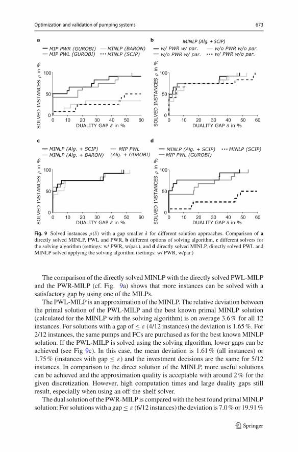
Optimization and validation of pumping systems 673
0 10 20 30 40 50 60DUALITY GAP in %
0
50
100
0 10 20 30 40 50 60DUALITY GAP in %
0
50
100
SO
LVED
IN
STA
NCES
in
%
SEC
NAT
SN I
D EVL
OS
in %
0 10 20 30 40 50 60DUALITY GAP in %
0
50
100
0 10 20 30 40 50 60DUALITY GAP in %
0
50
100
SO
LVED
IN
STA
NCES
in
%
SEC
NAT
SNI
DEVL
OS
in %
MINLP (BARON)MINLP (SCIP)
MIP PWR (GUROBI)MIP PWL (GUROBI)
w/ PWR w/ par.w/o PWR w/ par.
w/o PWR w/o par.w/ PWR w/o par.
MINLP (Alg. + SCIP)
MINLP (Alg. + SCIP) MINLP (SCIP)MIP PWL (GUROBI)MINLP (Alg. + BARON)
MIP PWL(Alg. + GUROBI)
a b
c d
MINLP (Alg. + SCIP)
Fig. 9 Solved instances ρ(δ) with a gap smaller δ for different solution approaches. Comparison of adirectly solved MINLP, PWL and PWR, b different options of solving algorithm, c different solvers forthe solving algorithm (settings: w/ PWR, w/par.), and d directly solved MINLP, directly solved PWL andMINLP solved applying the solving algorithm (settings: w/ PWR, w/par.)
The comparison of the directly solvedMINLP with the directly solved PWL-MILPand the PWR-MILP (cf. Fig. 9a) shows that more instances can be solved with asatisfactory gap by using one of the MILPs.
The PWL-MILP is an approximation of theMINLP. The relative deviation betweenthe primal solution of the PWL-MILP and the best known primal MINLP solution(calculated for the MINLP with the solving algorithm) is on average 3.6% for all 12instances. For solutions with a gap of ≤ ε (4/12 instances) the deviation is 1.65%. For2/12 instances, the same pumps and FCs are purchased as for the best known MINLPsolution. If the PWL-MILP is solved using the solving algorithm, lower gaps can beachieved (see Fig 9c). In this case, the mean deviation is 1.61% (all instances) or1.75% (instances with gap ≤ ε) and the investment decisions are the same for 5/12instances. In comparison to the direct solution of the MINLP, more useful solutionscan be achieved and the approximation quality is acceptable with around 2% for thegiven discretization. However, high computation times and large duality gaps stillresult, especially when using an off-the-shelf solver.
The dual solution of the PWR-MILP is comparedwith the best found primalMINLPsolution: For solutionswith a gap≤ ε (6/12 instances) the deviation is 7.0%or 19.91%
123
674 T. M. Müller et al.
(all instances) and investment decisions are the same for 5/12 of the instances. Thehigh deviation is due to non-converged solutions for difficult instances. In this case,the dual bound of the PWR-MILP cannot be raised sufficiently, which is why it servesonly as a weak lower bound.
Figure 9 further shows, that the difference between SCIP and BARON to directlysolve the MINLP is not significant. Both solvers can only solve 1/12 of the instanceswith a gap ≤ ε. In addition, we occasionally encountered errors with both solversduring the solution process. For SCIP this can be reduced by a less aggressive pre-solving. A more detailed discussion can be found in Appendix A. A direct solutionof the MINLP with off-the-shelf solvers is due to the large duality gap and potentialwrong results an unsuitable approach. In the solving algorithm the individual prob-lems are smaller and errors by SCIP or BARON were rare. However, for SCIP thepresolving-emphasis settings for the calculation with the solving algorithm were setto “fast” to avoid any problems.Performance of Solving Algorithm Fig. 9b shows the performance of the solving algo-rithm with and without the use of PWR (w/ PWR and w/o PWR) and parallelization(w/ par. and w/o par.). Without the use of PWR, the reduced MINLP is already solvedwithin the first selection of a tuple, thus the PWR-MILP is not solved before. Withoutparallelization, only one tuple is solved instead of N tuples at the same time. SCIP isused as MINLP solver and GUROBI as PWR-MILP solver. All in all, the deviationsof the different settings are rather small. The results show:
– The use of PWR shows only minor improvements. This could be caused by a toofine discretization, resulting in a dual bound of the PWR that can only be computedwith high effort.
– The parallelization offers a slight performance increase. The reason it only yieldssmall improvements could be that when solving N tuple at the same time, thecomputation of one tuple takes much longer than for the others. As long as thefirst N tuples are not finished, the primal and dual bounds are not updated. Thisholds the risk of wasting time on the computation of tuples which are cut off lateranyway. In addition, parallelization causes computational overhead.
In Fig. 9c, BARON and SCIP are compared as underlying MINLP solvers forthe solving algorithm (w/ PWR, w/ par.). The performance of SCIP is slightly bet-ter. In addition, the PWL-MILP is solved with the solving algorithm (GUROBI asPWL-MILP solver, w/o PWR, w/ par.). The performance is slightly below that of theMINLP. A possible cause is the computational overhead of the solving algorithm:The optimization model has to be set up for each tuple. This is more complex for thePWLmodel due to the increased number of equations, which can lead to a loss of per-formance. Nevertheless, compared to directly solving the PWL-MILP, considerablymore instances can be solved (cf. Fig. 9a).
Concluding, the results for the solving algorithm (SCIP, w/ PWR, w/ par.) are com-pared with directly solved MINLP and PWL-MILP in Fig. 9d: the solving algorithmallows to solve 50% of the instances with a gap ≤ ε and all instances with a gap ≤48%. This is substantially more than directly solving theMINLP and also than directlysolving the approximated PWL-MILP.
123
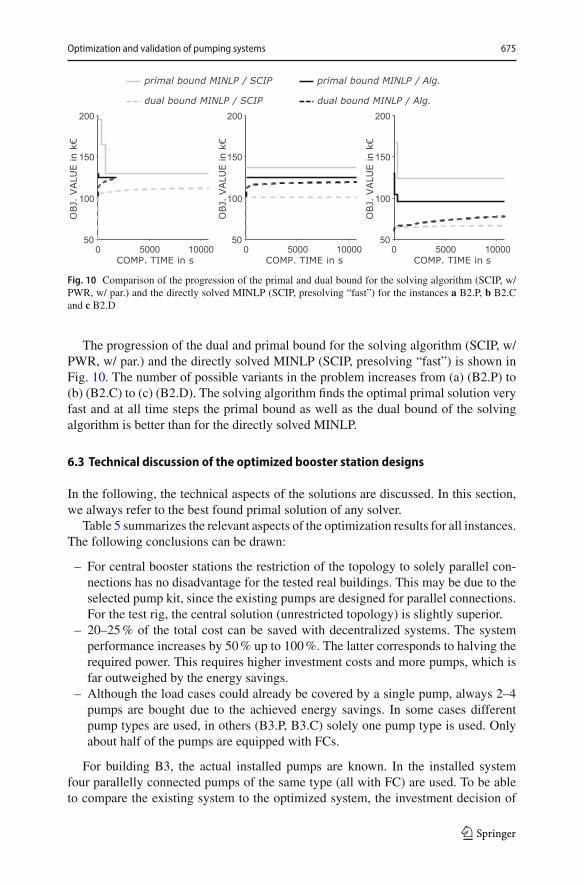
Optimization and validation of pumping systems 675
Fig. 10 Comparison of the progression of the primal and dual bound for the solving algorithm (SCIP, w/PWR, w/ par.) and the directly solved MINLP (SCIP, presolving “fast”) for the instances a B2.P, b B2.Cand c B2.D
The progression of the dual and primal bound for the solving algorithm (SCIP, w/PWR, w/ par.) and the directly solved MINLP (SCIP, presolving “fast”) is shown inFig. 10. The number of possible variants in the problem increases from (a) (B2.P) to(b) (B2.C) to (c) (B2.D). The solving algorithm finds the optimal primal solution veryfast and at all time steps the primal bound as well as the dual bound of the solvingalgorithm is better than for the directly solved MINLP.
6.3 Technical discussion of the optimized booster station designs
In the following, the technical aspects of the solutions are discussed. In this section,we always refer to the best found primal solution of any solver.
Table 5 summarizes the relevant aspects of the optimization results for all instances.The following conclusions can be drawn:
– For central booster stations the restriction of the topology to solely parallel con-nections has no disadvantage for the tested real buildings. This may be due to theselected pump kit, since the existing pumps are designed for parallel connections.For the test rig, the central solution (unrestricted topology) is slightly superior.
– 20–25% of the total cost can be saved with decentralized systems. The systemperformance increases by 50% up to 100%. The latter corresponds to halving therequired power. This requires higher investment costs and more pumps, which isfar outweighed by the energy savings.
– Although the load cases could already be covered by a single pump, always 2–4pumps are bought due to the achieved energy savings. In some cases differentpump types are used, in others (B3.P, B3.C) solely one pump type is used. Onlyabout half of the pumps are equipped with FCs.
For building B3, the actual installed pumps are known. In the installed systemfour parallelly connected pumps of the same type (all with FC) are used. To be ableto compare the existing system to the optimized system, the investment decision of
123

676 T. M. Müller et al.
Table 5 Results of the best found primal solution for each instance
building B1 building B2parallel central decen. parallel central decen
total cost in ke 141.7 141.7 107.4 124.4 124.4 93.9
rel. total cost in % 100 100 75.8 100 100 75.5
invest. cost in ke 32.4 32.4 34.7 30.3 30.3 32.4
# pumps 3 3 4 2 2 4
# diff. types 2 2 4 2 2 4
# FC 1 1 3 1 1 2
mean power in kW 10.9 10.9 7.2 9.3 9.3 6.1
η1sys in % 37.8 37.8 56.9 36.6 36.7 56.1
building B3 test rig TREparallel central decen. inst. parallel central decen.
total cost in e 16377 16377 12715 24391 957 933 780
rel. total cost in % 100 100 77.6 148.9 100 97.5 81.5
invest. cost in e 6321 6321 7762 14868 276 244 226
# pumps 2 2 4 4 2 2 2
# diff. types 1 1 2 1 2 2 2
# FC 1 1 2 4 – – –
mean power in W 998 998 491 947 67.6 68.4 55
η1sys in % 22.4 22.4 45.5 23.64 25.7 25.4 31.5
The system efficiency is defined as: ηsys := Pomeanhydr,dec.Pomean
=∑
s∈S Ws Pos,hydr,dec.∑s∈S Ws
∑i∈P poi,s
the existing system is fixed and the rotational speed optimized (see column “inst.” inTable 5). In comparison, approx. 50% of the total cost can be saved by optimizing theinvestment costs and speed at the same time. Even if costs for an additional redundantspare pump are taken into account (2053 e, without FC), 32% of the total cost canstill be saved.
All selected pumps are highlighted in Fig. 11. Solid black lines indicate pumps,that are selected for any setting, while dashed black lines indicate pumps that are onlyselected for decentralized settings.
For building B1, the optimal topologies are shown in Fig. 12. The central topology(a) shows that only the largest pump is equipped with a frequency converter andoperates for every load scenarios. For the load cases with higher power demand,further pumps are switched on additionally. An interpretation of this chosen topologycan be that the additional pumps run for a small part of the operation time only andtherefore their energy consumption and resulting costs do not weigh enough to equipeither of these pumps with a frequency converter. A complex topology results for thedecentralized solution (b). In scenarios with low hydraulic power demand, one pumpsolely supplies the pressure zones 1 and 2. Two pumps connected in series supply theupper pressure zones. After the first pump a partial volume flow is branched off to
123
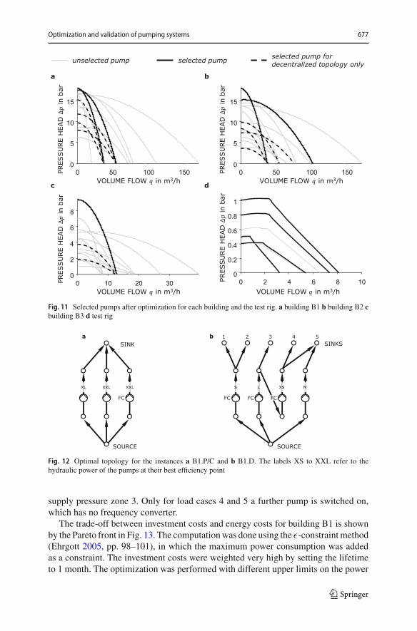
Optimization and validation of pumping systems 677
0 2 4 6 8 100
0.2
0.4
0.6
0.8
1
VOLUME FLOW in m3/h
PRES
SU
RE
HEA
D Δ
in b
ar
0 50 100 150VOLUME FLOW in m3/h
0
5
10
15
PRES
SU
RE
HEA
D Δ
in b
ar
0 10 20 30VOLUME FLOW in m3/h
0
2
4
6
8
DAE
HE
RU
SSE
RPΔ
r abn i
0 50 100 150VOLUME FLOW in m3/h
0
5
10
15
DAE
HE
RU
SSE
R PΔ
rabni
c d
ba
unselected pump selected pump selected pump fordecentralized topology only
Fig. 11 Selected pumps after optimization for each building and the test rig. a building B1 b building B2 cbuilding B3 d test rig
SOURCE
S L XS M
SINKS1 2 3 54
XL XXL
SOURCE
XXL
SINKa b
FC FC FCFC
Fig. 12 Optimal topology for the instances a B1.P/C and b B1.D. The labels XS to XXL refer to thehydraulic power of the pumps at their best efficiency point
supply pressure zone 3. Only for load cases 4 and 5 a further pump is switched on,which has no frequency converter.
The trade-off between investment costs and energy costs for building B1 is shownby the Pareto front in Fig. 13. The computationwas done using the ε-constraintmethod(Ehrgott 2005, pp. 98–101), in which the maximum power consumption was addedas a constraint. The investment costs were weighted very high by setting the lifetimeto 1 month. The optimization was performed with different upper limits on the power
123
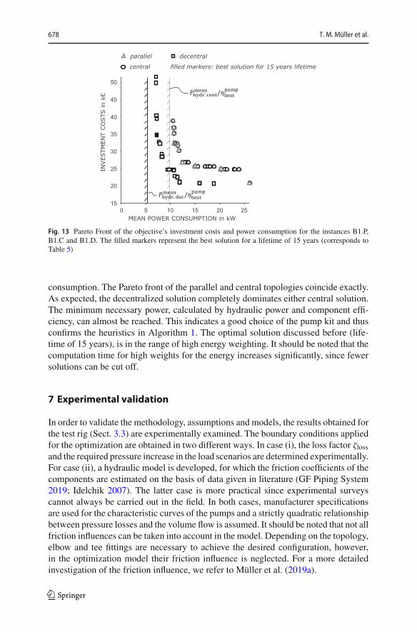
678 T. M. Müller et al.
Fig. 13 Pareto Front of the objective’s investment costs and power consumption for the instances B1.P,B1.C and B1.D. The filled markers represent the best solution for a lifetime of 15 years (corresponds toTable 5)
consumption. The Pareto front of the parallel and central topologies coincide exactly.As expected, the decentralized solution completely dominates either central solution.The minimum necessary power, calculated by hydraulic power and component effi-ciency, can almost be reached. This indicates a good choice of the pump kit and thusconfirms the heuristics in Algorithm 1. The optimal solution discussed before (life-time of 15 years), is in the range of high energy weighting. It should be noted that thecomputation time for high weights for the energy increases significantly, since fewersolutions can be cut off.
7 Experimental validation
In order to validate the methodology, assumptions and models, the results obtained forthe test rig (Sect. 3.3) are experimentally examined. The boundary conditions appliedfor the optimization are obtained in two different ways. In case (i), the loss factor ζlossand the required pressure increase in the load scenarios are determined experimentally.For case (ii), a hydraulic model is developed, for which the friction coefficients of thecomponents are estimated on the basis of data given in literature (GF Piping System2019; Idelchik 2007). The latter case is more practical since experimental surveyscannot always be carried out in the field. In both cases, manufacturer specificationsare used for the characteristic curves of the pumps and a strictly quadratic relationshipbetween pressure losses and the volume flow is assumed. It should be noted that not allfriction influences can be taken into account in the model. Depending on the topology,elbow and tee fittings are necessary to achieve the desired configuration, however,in the optimization model their friction influence is neglected. For a more detailedinvestigation of the friction influence, we refer to Müller et al. (2019a).
123

Optimization and validation of pumping systems 679
XL L XL M L S S XL S
SINKS1 2 3 54
SOURCE SOURCE SOURCESOURCE
SINKSINKSINKa b dc
Fig. 14 Optimal topology for the test rig: a parallel (experimental data as well as solely literature data), bcentral (experimental data), c central (solely literature data) and d decentral (experimental data as well assolely literature data). For topology c the setup on the test rig is shown in Fig. 3
The optimal topologies are shown in Fig. 14. Only for the central booster station(b)/(c) there are deviations in the optimal topology between experimental and literaturedata.Without the use of experimental data, the pressure losses are assumed to be lower,which is why slower rotational speeds are applied.
The shown topologies are set up on the test rig, trying to keep the pressure losses dueto the layout of the connections as low as possible. For every scenario the rotationalspeeds are applied and the valves are set so that the same volume flow is achieved oneach floor. The pumps run at a constant speed, i.e. without pressure or volume flowcontrol-loop.
In Fig. 15, the power consumption (measure for the achievement of the objective)is plotted against the volume flow (measure for the satisfaction of the load demand)for all topologies and scenarios.
The correlation between power and volume flow is well matched in computationand experiment even though there is a deviation between the required and themeasuredvolume flows. As expected, the correlation is higher when using the experimental data.
Furthermore, the mean volume flow,
Qmean :=∑
s∈SWs
∑
f ∈Fq f ,s, (17)
the mean power consumption,
Pomean :=∑
s∈SWs
∑
i∈Ppoi,s, (18)
123

680 T. M. Müller et al.
optimization validation
0 2 4VOLUME FLOW in m³/h
0
50
100
150
200
250
0 2 4VOLUME FLOW in m³/h
0
50
100
150
200
250
0 2 4VOLUME FLOW in m³/h
0
50
100
150
200
250
0 2 4VOLUME FLOW in m³/h
0
50
100
150
200
250
0 2 4VOLUME FLOW in m³/h
0
50
100
150
200
250
0 2 4VOLUME FLOW in m³/h
0
50
100
150
200
250
REW
OPW
niRE
WOP
Wni
POW
ERin
WPO
WER
in W
POW
ERin
WPO
WER
in W
a b
d
c
e f
Fig. 15 Power consumption over volume flow for optimization and validation results for all five loadscenarios. Results based on experimental data for a parallel b central and c decentral topologies, and basedon literature data for d parallel e central and f decentral topologies are shown. The error bars are coveredby the markers
and the geodetic system efficiency are investigated cf. Table 6,
ηgeo :=∑
s∈S Ws�g∑
f ∈F Δh f q f ,s
Pomean. (19)
The values are calculated using the density � = 998 kgm−3, the gravitational accel-eration g = 9.81m s−2, and the geodetic height differenceΔh f = {1m, . . . , 5m} forthe different pressure zones. The geodetic system efficiency ηgeo is a measure for thedeviation of the energy costs and is used to determine the expected total cost:
Cexptotal := Copt
invest + Coptenergy
(1 + η
optgeo − η
expgeo
ηoptgeo
). (20)
The results show that the mean volume flow is higher than demanded, i.e. the pressurelosses have been overestimated. As a result, the power consumption is also higherthan predicted. In practice, the deviations would be compensated by a closed loopcontrol of each pump’s rotational speed. The systems are nevertheless comparableon the basis of the geodetic efficiency, which is slightly lower than assumed in theoptimization. The deviation is smaller for the pump model based on the experimentaldata. For the instanceswhere the pumpSwas installed (cf. Fig. 14b and c), the deviationis higher, which indicates inaccuracies in the used characteristics of pump S (givenby the manufacturers data sheet). In spite of these uncertainties, the total costs arelower for decentralized systems. The deviations in efficiency (5-10%) are significantly
123
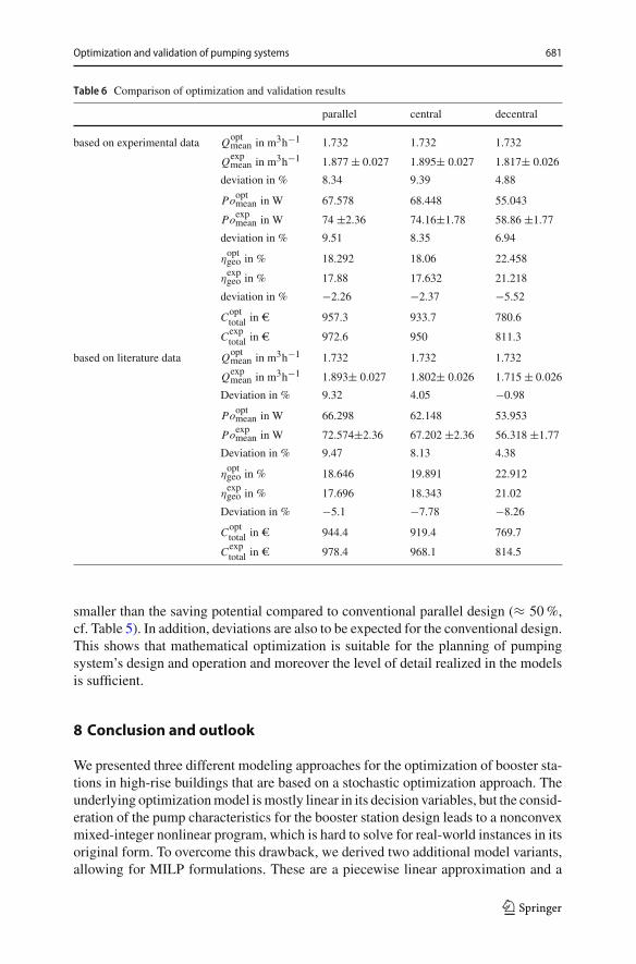
Optimization and validation of pumping systems 681
Table 6 Comparison of optimization and validation results
parallel central decentral
based on experimental data Qoptmean in m3h−1 1.732 1.732 1.732
Qexpmean in m3h−1 1.877 ± 0.027 1.895± 0.027 1.817± 0.026
deviation in % 8.34 9.39 4.88
Pooptmean in W 67.578 68.448 55.043
Poexpmean in W 74 ±2.36 74.16±1.78 58.86 ±1.77
deviation in % 9.51 8.35 6.94
ηoptgeo in % 18.292 18.06 22.458
ηexpgeo in % 17.88 17.632 21.218
deviation in % −2.26 −2.37 −5.52
Copttotal in e 957.3 933.7 780.6
Cexptotal in e 972.6 950 811.3
based on literature data Qoptmean in m3h−1 1.732 1.732 1.732
Qexpmean in m3h−1 1.893± 0.027 1.802± 0.026 1.715 ± 0.026
Deviation in % 9.32 4.05 −0.98
Pooptmean in W 66.298 62.148 53.953
Poexpmean in W 72.574±2.36 67.202 ±2.36 56.318 ±1.77
Deviation in % 9.47 8.13 4.38
ηoptgeo in % 18.646 19.891 22.912
ηexpgeo in % 17.696 18.343 21.02
Deviation in % −5.1 −7.78 −8.26
Copttotal in e 944.4 919.4 769.7
Cexptotal in e 978.4 968.1 814.5
smaller than the saving potential compared to conventional parallel design (≈ 50%,cf. Table 5). In addition, deviations are also to be expected for the conventional design.This shows that mathematical optimization is suitable for the planning of pumpingsystem’s design and operation and moreover the level of detail realized in the modelsis sufficient.
8 Conclusion and outlook
We presented three different modeling approaches for the optimization of booster sta-tions in high-rise buildings that are based on a stochastic optimization approach. Theunderlying optimizationmodel ismostly linear in its decision variables, but the consid-eration of the pump characteristics for the booster station design leads to a nonconvexmixed-integer nonlinear program, which is hard to solve for real-world instances in itsoriginal form. To overcome this drawback, we derived two additional model variants,allowing for MILP formulations. These are a piecewise linear approximation and a
123
682 T. M. Müller et al.
piecewise linear relaxation of the nonlinear pump characteristics. Furthermore, weimplemented a problem-specific solving algorithm which is based on these differentmethods and additional domain-specific engineering knowledge to derive global-optimal results for real-world instances efficiently. The solving algorithm reducesthe original MINLP by fixing specific pump purchase decisions and uses a selectionheuristic to find feasible primal solutions in a very short time. This primal solutionsearch is undertaken alternating with the dual solution search, which is based either onthe reduced MINLP directly or on the implemented piecewise linear relaxation. Thepresented solving algorithm improves the solution times considerably in comparisonto the originalMINLP formulation.We presented the computation benefits of the solv-ing algorithm for three different high-rise buildings as well as for a test rig. The test rig,constructed for validation purposes, represents the scaled water supply in a high-risebuilding. Therefore, we were able to conduct experiments for results of the optimiza-tion models considering different data sources as well as varying degrees of freedom.The comparison of optimization and experimental results on the test rig shows that thedegree of detail is adequate and that the introducedmethod is transferable to real-worldinfrastructure. Allowing for different degrees of freedom for the alignment of pumpsin the water supply system shows that the decentralized topology of booster stationscan yield approx. 25% of cost savings when compared to an optimized parallel pumpalignment. The latter design is the current common practice. Additionally, frequencyconverters were installed for only approx. half of the pumps in booster stations, whichis due to the trade-off of energy costs in operation and investment costs making uptotal cost. Compared to a conventionally designed booster station, the mathematicaloptimization could achieve a total cost reduction of up to approx. 50%. These resultsshow that we were able to derive significantly improved system designs by combin-ing domain-specific engineering knowledge and discrete optimization methods. Thedeveloped approach assists engineers as early as in the design stage to improve thesystem design. This is possible, since this approach allows to consider the real loadprofile in the implemented two-stage stochastic optimization problem. For the future,we want to address further open research questions in this area, both in the algorith-mic and engineering domain. For instance, to obtain reasonable problem sizes, we hadto reduce the number of different pump types in the preprocessing with the help ofan engineering knowledge applying heuristic. Therefore, improving the performanceof the algorithm to consider more pumps could achieve even better system designs.This objective could be approached by an improved deployment of the underlyingpiecewise relaxation or by warm-starting already investigated subproblems. From anengineering perspective, we want to examine more complex, branched systems andwant to look into the transfer of the methods to different fluid systems. Finally, wewould like to examine the operation in more detail and ensure that the best possi-ble performance is achieved even with load variations and deviations of the assumedparameters.
Acknowledgements The presented results were partly obtained within the research project “Exact GlobalTopology-Optimization for Pumping Systems”, Project No. 19725 N/1, funded by the program for pro-moting the Industrial Collective Research (IGF) of the German Ministry of Economic Affairs and Energy(BMWi), approved by the Arbeitsgemeinschaft industrieller Forschungsvereinigungen “Otto von Guer-icke” e.V. (AiF). We want to thank all the participants of the working group for the constructive and close
123

Optimization and validation of pumping systems 683
collaboration. Moreover, we thank the German Research Foundation, DFG, for partial funding within theCollaborative Research Center CRC 805 “Control of Uncertainties in Load-Carrying Structures inMechan-ical Engineering”, Project No. 57157498. In addition to that, we appreciate the partial funding by the KSBStiftung Stuttgart, Germany.
Funding Open Access funding provided by Projekt DEAL.
OpenAccess This article is licensedunder aCreativeCommonsAttribution 4.0 InternationalLicense,whichpermits use, sharing, adaptation, distribution and reproduction in any medium or format, as long as you giveappropriate credit to the original author(s) and the source, provide a link to the Creative Commons licence,and indicate if changes were made. The images or other third party material in this article are includedin the article’s Creative Commons licence, unless indicated otherwise in a credit line to the material. Ifmaterial is not included in the article’s Creative Commons licence and your intended use is not permittedby statutory regulation or exceeds the permitted use, you will need to obtain permission directly from thecopyright holder. To view a copy of this licence, visit http://creativecommons.org/licenses/by/4.0/.
A Appendix
Within the computational evaluations we encountered problems with the two MINLPsolvers SCIP (v5.0) and BARON (v.19.7.13), which we present in more detail in thefollowing.Within modeling, we put a lot of effort in the conditioning of the underlyingoptimization problem to reduce errors based on an ill-conditioned optimization prob-lem. A summary can be found in Table 7. While BARON occasionally generated nooutput for specific instances, SCIP either indicated larger dual bounds than the valueof the true primal solutions or declared instances as infeasible while we were able toderive feasible solutions either with BARON or manually by engineering knowledge.BARON terminated without solution output for 4/12 instances for the original MINLPgiven by (5) and (6). SCIP output an incorrect solution for 5/12 instances in the originalMINLP with default presolving settings. We were able to reduce the number of falseresults for SCIP by adjusting the presolving emphasis settings to “fast” or “off”, asindicated in Table 7. A newer version of SCIP or BARON can potentially solve theencountered issues.
Table 7 Specification of the instances for which an error occurred in the direct solution of the MINLPs
Presolving emphasis settings BARON SCIPDefault Default Fast Off
No output B1.P, B1.D, B2.C, B2.D – – B1.P
Wrongly detected infeasibility – B1.P, B1.D, B3.P – TE.D
Indicated too large dual bound – B3.C, B3.D B2.P –
# Instances with error 4/12 5/12 1/12 2/12
123
684 T. M. Müller et al.
References
AfA table (1995) Afa table for the branch energy and water supply. (tax depreciation for wear and tear).File number IV A 8-S 1551-9/95, 45-S 1551-20
Altherr LC, Leise P, PfetschME, Schmitt A (2019) Resilient layout, design and operation of energy-efficientwater distribution networks for high-rise buildings using MINLP. Optimiz Eng 20(2):605–645
Brennen CE (2011) Hydrodynamics of pumps. Cambridge University Press, CambridgeBundesbank (2019) Discount rates in accordance with section 253 (2) HGB, 7-year average, remaining
time 15 years. Time series BBK01.WX0037Carøe CC, Tind J (1998) L-shaped decomposition of two-stage stochastic programs with integer recourse.
Math Program 83(1–3):451–464Coelho B, Andrade-Campos A (2014) Efficiency achievement in water supply systems—a review. Renew
Sustain Energy Rev 30:59–84CTBUH (2018) tall building year in review. Technical report, Council on Tall Buildings and Urban HabitatCurrie J,WilsonDI, Sahinidis N, Pinto J (2012) OPTI: Lowering the barrier between open source optimizers
and the industrial MATLAB user. https://www.inverseproblem.co.nz/OPTI/. Accessed Oct 29th 2019Destatis (2019) Daten zur Energiepreisentwicklung. Lange Reihen von Januar 2005 bis August 2019DIN 1988-300 (2012) Codes of practice for drinking water installations—Part 300: Pipe sizing; DVGW
code of practiceDIN 1988–500 (2011) Codes of practice for drinking water installations—Part 500: Pressure boosting
stations with RPM-regulated pumps; DVGW code of practiceEhrgott M (2005) Multicriteria optimization, vol 2. Springer, BerlinEN 16480:2016 (2016) Pumps–minimum required efficiency of rotodynamic water pumpsFerreira FJ, Fong JA, de Almeida AT (2010) Ecoanalysis of variable-speed drives for flow regulation in
pumping systems. IEEE Trans Ind Electron 58(6):2117–2125Fisher DS (2001) The impact of safety factors on pump performance and selection: Case study, a method-
ology for correcting pump oversizing/discussion. ASHRAE Trans 107:584Garg VK (1998) Applied computational fluid dynamics. CRC Press, Boca RatonGeißler B, Martin A, Morsi A, Schewe L (2012) Using piecewise linear functions for solving MINLPs. In:
Lee J, Leyffer S (eds) Mixed integer nonlinear programming. Springer, New York, pp 287–314GF Piping System (2019) JRG Sanipex MT - Technical documentation. https://www.gfps.com/appgate/
ecat/common_flow/10006Q/CH/en/231565/download/document.html. Accessed Oct 30th 2019Gleixner A, Eifler L, Gally T, Gamrath G, Gemander P, Gottwald RL, Hendel G, Hojny C, Koch T, Mil-
tenberger M, Müller B, Pfetsch ME, Puchert C, Rehfeldt D, Schlösser F, Serrano F, Shinano Y,Viernickel JM, Vigerske S, Weninger D, Witt JT, Witzig J (2017) The SCIP Optimization Suite5.0. Technical report, Optimization Online, http://www.optimization-online.org/DB_HTML/2017/12/6385.html. Accessed Oct 29th 2019
Gössling S, Peeters P, Hall CM, Ceron JP, Dubois G, Scott D et al (2012) Tourism and water use: supply,demand, and security. an international review. Tourism Manage 33(1):1–15
Groß T, Pöttgen P, Pelz PF (2017) Analytical approach for the optimal operation of pumps in boostersystems. J Water Resour Plan Manage 143(8):04017029
Grundfos Pumps Ltd (2016) Pressure booster pumps and sets 2016 range overview. https://uk.grundfos.com/content/dam/UK/Brochure/Booster%20overview/Booster%20Pumps%20Brochure%20May%202016.pdf. Accessed March 4th 2020
Gülich JF (2010) Centrifugal pumps. Springer, BerlinGUROBI (2020) GUROBI Optimization. http://www.gurobi.com. Accessed March 24th 2020Hartisch M, Herbst A, Lorenz U, Weber JB (2018) Towards resilient process networks-designing booster
stations via quantified programming. Appl Mech Mater Trans Tech Publ 885:199–210Herrera M, Abraham E, Stoianov I (2016) A graph-theoretic framework for assessing the resilience of
sectorised water distribution networks. Water Resour Manage 30(5):1685–1699Hirschberg R (2014) Lastprofil und Regelkurve zur energetischen Bewertung von Druckerhöhungsanlagen
(DEA). HLH Lüftung/Klima, Heizung/Sanitär, Gebäudetechnik pp 1436–5103Humpola J, Fügenschuh A (2015) Convex reformulations for solving a nonlinear network design problem.
Comput Optim Appl 62(3):717–759IBM (2020) IBM ILOG CPLEX Optimization Studio. https://www.ibm.com/products/ilog-cplex-
optimization-studio. Accessed March 24th 2020Idelchik IE (2007) Handbook of hydraulic resistance, 4th edn. Begell House, New York
123

Optimization and validation of pumping systems 685
ISO/ASME 14414 (2019) Pump system energy assessmentJapikse D, Marscher WD, Furst RB (1997) Centrifugal pump design and performance. Concepts ETI Inc,
WilderKSB SE Co KGaA (2020) Hyamat SVP pressure boosting units. https://products.ksb.com/global/products/
pumps-and-pump-systems/ready-to-connect-pump-sets/pressure-boosting-units/hyamat-svp-3014.Accessed March 4th 2020
Lang S, Ludwig G, Pelz PF, Stoffel B (2013) General methodologies of determining the energy-efficiency-index of pump units in the frame of the extended product approach. In: Proceedings of the 8thinternational conference on energy efficiency in motor driven systems (EEMODS)
Larralde E, Ocampo R (2010a) Centrifugal pump selection process. World Pumps 2010(2):24–28Larralde E, Ocampo R (2010) Pump selection: a real example. World Pumps 3:28–33Leise P, Altherr LC (2018) Optimizing the design and control of decentralized water supply systems – A
case-study of a hotel building. In: International conference on engineering optimization, Springer, pp1241–1252
Löfberg J (2004) YALMIP: A toolbox for modeling and optimization in MATLAB. In: Proceedings of theCACSD conference
Meck M, Müller TM, Altherr LC, Pelz PF (2019) Designing an Efficient and Cost-Optimal IndustrialCooling System Using Mixed-Integer Nonlinear Programming. In: Operations research proceedings2019, Springer, to appear
Mikolajková M, Saxén H, Pettersson F (2018) Linearization of an MINLP model and its application to gasdistribution optimization. Energy 146:156–168
Misener R, Floudas CA (2010) Piecewise-linear approximations of multidimensional functions. J OptimTheory Appl 145(1):120–147. https://doi.org/10.1007/s10957-009-9626-0
Misener R, Floudas CA (2012) Global optimization of mixed-integer quadratically-constrained quadraticprograms (MIQCQP) through piecewise-linear and edge-concave relaxations. Math Program136(1):155–182
Misener R, Floudas CA (2013) GloMIQO: global mixed-integer quadratic optimizer. J Global Optim57(1):3–50
Misener R, Floudas CA (2014) ANTIGONE: algorithms for continuous/integer global optimization ofnonlinear equations. J Global Optim 59(2–3):503–526
Misener R, Gounaris CE, Floudas CA (2009) Global optimization of gas lifting operations: a comparativestudy of piecewise linear formulations. Ind Eng Chem Res 48(13):6098–6104
MorsiA,GeißlerB,MartinA (2012)Mixed integer optimization ofwater supply networks. In:Mathematicaloptimization of water networks. Springer, pp 35–54
Müller TM, Altherr LC, Leise P, Pelz PF (2019a) Optimization of pumping systems for buildings: Exper-imental validation of different degrees of model detail on a modular test rig. In: Operations researchproceedings 2019, Springer, Dresden, Germany, to appear
Müller TM, Leise P, Meck T, Altherr LC, Pelz PF (2019b) Systemic optimization of booster stations—fromdata collection to validation. In: International rotating equipment conference (IREC) 2019,Wiesbaden,Germany
Norgaard J, NielsenA (2010)Water supply in tall buildings: roof tanks versus pressurised systems.GrundfosWater Boosting, Denmark
Nowak D, Krieg H, Bortz M, Geil C, Knapp A, Roclawski H, Böhle M (2018) Decision support for thedesign and operation of variable speed pumps in water supply systems. Water 10(6):1
Pecci F, Abraham E, Stoianov I (2019) Global optimality bounds for the placement of control valves inwater supply networks. Optim Eng 20(2):457–495. https://doi.org/10.3390/w10060734
Pedersen GK, Yang Z (2008) Efficiency optimization of a multi-pump booster system. In: Proceedings ofthe 10th annual conference on genetic and evolutionary computation, ACM, pp 1611–1618
Popela P (2010) Stochastic programmingmodels for engineering design problems. EngMech 17(5–6):351–362
Popela P, Novotny J, Roupec J, Hrabec D, Olstad A (2014) Two-stage stochastic programming for engi-neering problems. Eng Mech 21(5):335–353
Puranik Y, Sahinidis NV (2017) Domain reduction techniques for global NLP and MINLP optimization.Constraints 22(3):338–376
Rausch L, Leise P, Ederer T, Altherr LC, Pelz PF (2016) A comparison of MILP and MINLP solverperformance on the example of a drinking water supply system design problem. In: Proceedings of
123

686 T. M. Müller et al.
the European congress on computational methods in applied sciences and engineering, Crete Island,Greece, pp 5–10
Schultz R (1992) Continuity and stability in two-stage stochastic integer programming. In: StochasticOptimization, Springer, pp 81–92
Stoffel B (2015) Assessing the energy efficiency of pumps and pump units. Elsevier, AmsterdamTawarmalani M, Sahinidis NV (2005) A polyhedral branch-and-cut approach to global optimization. Math
Program 103:225–249Tindall J, Pendle J (2015) Are we significantly oversizing domestic water systems? In: CIBSE Technical
Symposium 2015, 16th–17th April 2015, UCL LondonTolvanen J (2007) Life cycle energy cost savings through careful system design and pump selection. World
Pumps 2007(490):34–37Ulanicki B, Kahler J, Coulbeck B (2008) Modeling the efficiency and power characteristics of a pump
group. J Water Resour Plan Manage 134(1):88–93UN (2018) 2018 revision of world urbanization prospects. Tech. rep, United NationsVielma JP, Ahmed S, Nemhauser G (2010) Mixed-integer models for nonseparable piecewise-linear opti-
mization: Unifying framework and extensions. Oper Res 58(2):303–315Wächter A, Biegler LT (2006) On the implementation of an interior-point filter line-search algorithm for
large-scale nonlinear programming. Math Program 106(1):25–57Weber JB, Lorenz U (2017) Optimizing booster stations. In: Proceedings of the genetic and evolutionary
computation conference companion, ACM, pp 1303–1310Weber JB, Lorenz U (2018) Algorithmic system design of thermofluid systems. In: International conference
on engineering optimization, Springer, pp 132–143Wets RJB (1974) Stochastic programs with fixed recourse: the equivalent deterministic program. SIAM
Rev 16(3):309–339Wilo SE (2020) Products and expertise for pressure boosting. https://wilo.com/ie/en/Products-and-
expertise/Product-Data/Pressure-boosting_32.html. Accessed March 4th 2020Zuse Institute Berlin (2020) Sequential object-oriented simPlex. https://soplex.zib.de/. Accessed March
24th 2020
Publisher’s Note Springer Nature remains neutral with regard to jurisdictional claims in published mapsand institutional affiliations.
123