Certain materials are included under the fair use exemption of the U.S. Copyright Law and have been prepared according to the fair use guidelines and are restricted from further use.

Project Number: AE- IIH-0003

Optimization and Control Design of an Autonomous Underwater Vehicle

A Major Qualifying Project Report:

submitted to the Faculty

of the

WORCESTER POLYTECHNIC INSTITUTE

in partial fulfillment of the requirements for the

Degree of Bachelor of Science

in Aerospace Engineering

by Daniel Moussette

Ashish Palooparambil

Jarred Raymond

Date: Thursday, April 29, 2010

Approved:

Professor Islam Hussein, Major Advisor

Keywords Professor William Michalson, Co-Advisor

1. Autonomous 2. Submarine 3. Hydrodynamic

i

Abstract

Autonomous vehicles are increasingly being investigated for use in oceanographic studies,

underwater surveillance, and search operations. Research currently being done in the area of

autonomous underwater craft is often hindered by expense. This project seeks to complete the

construction, optimization, and control software development of an inexpensive miniature underwater

vehicle. During the course of the project all of the vehicle’s mechanical and electrical subsystems were

completed. Propeller-driven primary thrusters using a magnetically coupled drive system were

optimized and manufactured. A battery powered electrical subsystem was also designed and installed

on the vehicle. A simulation of the vehicle’s control algorithm was developed in MATLAB and several full

vehicle tests were conducted in the WPI swimming pool.

ii

Executive Summary

The primary objective for the 2009-2010 Autonomous Underwater Vehicle (AUV) Major

Qualifying Project (MQP) was to program, optimize, and complete work on an existing submersible

platform built by the AUV MQP group from the 2008-2009 school year. Upon completion, this vehicle

will provide a low cost, highly adaptable platform for testing autonomous software and hardware. There

are AUV platforms available commercially, however they are typically too costly or not adaptable

enough to test various systems.

In order to complete the objective the group fabricated and optimized various hardware and

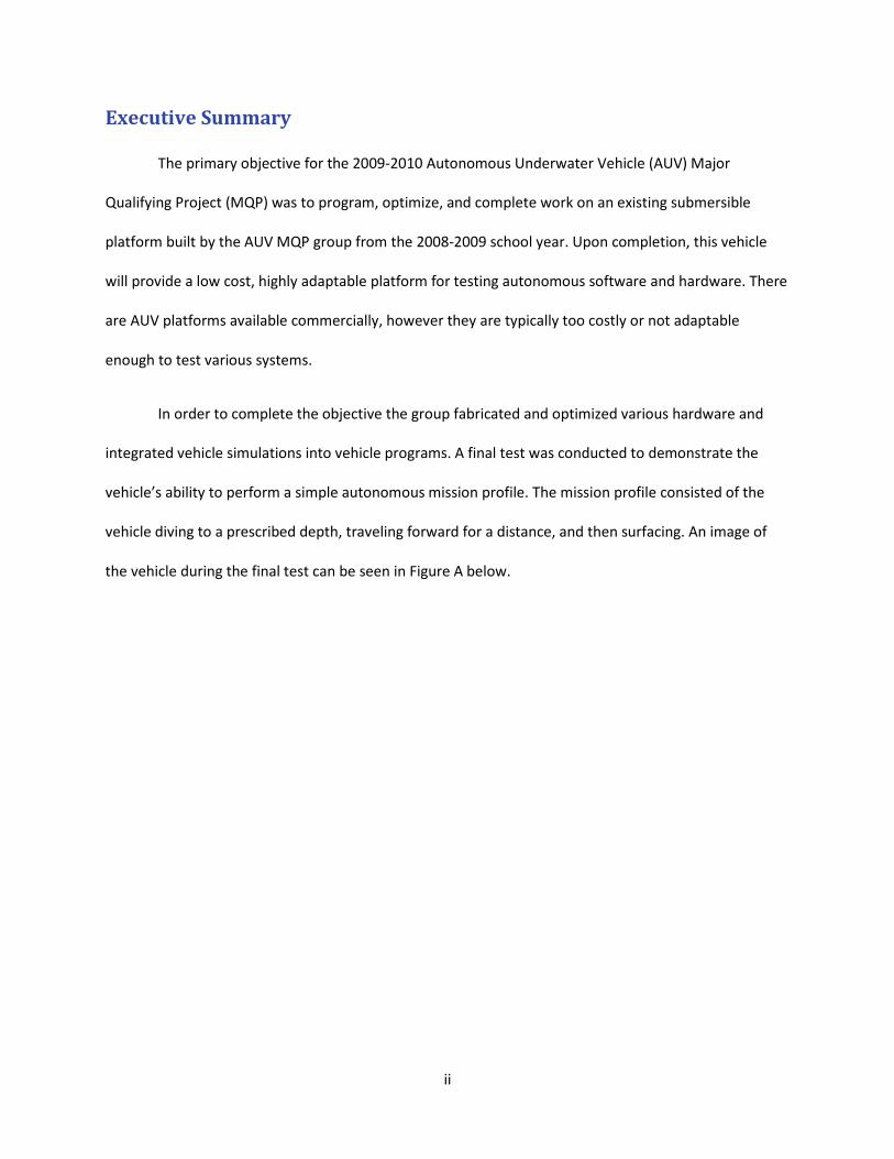
integrated vehicle simulations into vehicle programs. A final test was conducted to demonstrate the

vehicle’s ability to perform a simple autonomous mission profile. The mission profile consisted of the

vehicle diving to a prescribed depth, traveling forward for a distance, and then surfacing. An image of

the vehicle during the final test can be seen in Figure A below.

iii

Figure A: Vehicle during Final Mission Testing

Additional work is required to complete the control algorithms and integrate sensor systems in

the vehicle. Once complete, the vehicle should display full autonomy in all operations in the water.

These additional efforts will eventually allow the vehicle to perform more complex missions such as

searching for foreign objects or communicating with other autonomous vehicles.

iv

Acknowledgements

We would like to thank Professor Islam Hussein and Professor William Michalson for their

guidance and expertise throughout the duration of this project, Neil Whitehouse for his assistance in

manufacturing components, Tanvir Anjum for his assistance with the electronics and programming, and

Russel Morrin for his technical guidance.

v

Nomenclature

AC Alternating Current

ADC Analog to Digital Converter

AFL Actuator Front Left

AFR Actuator Front Right

Ah Ampere-Hour

ARL Actuator Rear Left

ARR Actuator Rear Right

ATX Advanced Technology Extended

C Celsius

DAC Digital to Analog Converter

DC Direct Current

E Volts

F Fahrenheit

FDS Front Drain Solenoid

FFS Front Fill Solenoid

Gb Gigabyte

GHz Gigahertz

I Amperes

I/O Input/Output

I2C Inter Integrated Circuit Control

L Inductance

m Meters

vi

m/s Meters per Second

MOSFET Metal-Oxide-Semiconductor Field Effect Transistor

n Turns ratio

N Number of turns

P Power

PCB Printed Circuit Board

PTL Primary Thruster Left

PTR Primary Thruster Right

RDS Rear Drain Solenoid

RFS Rear Fill Solenoid

s Seconds

SPI Serial Peripheral Interface

V Volts

W Watts

Wh Watt-Hour

WPI Worcester Polytechnic Institute

Z Impedance

vii

Table of Contents

ABSTRACT ............................................................................................................................................................... I

EXECUTIVE SUMMARY ........................................................................................................................................... II

ACKNOWLEDGEMENTS ......................................................................................................................................... IV

NOMENCLATURE ................................................................................................................................................... V

TABLE OF CONTENTS ............................................................................................................................................ VII

TABLE OF FIGURES ................................................................................................................................................. X

LIST OF TABLES .................................................................................................................................................... XII

1 INTRODUCTION ............................................................................................................................................ 1

2 BACKGROUND INFORMATION ...................................................................................................................... 4

2.1 VEHICLE HULL DESIGN ........................................................................................................................................... 5

2.2 FLUID SYSTEMS .................................................................................................................................................... 7

2.3 THRUSTER SYSTEMS .............................................................................................................................................. 8

2.3.1 Stabilizing Thrusters ............................................................................................................................... 9

2.3.2 Main Thrusters ..................................................................................................................................... 10

2.4 BALLAST SYSTEM ................................................................................................................................................ 10

2.5 POWER SYSTEM ................................................................................................................................................. 13

2.6 ELECTRONICS ..................................................................................................................................................... 14

2.6.1 Central Processing (PC/104 Stack) ...................................................................................................... 15

2.6.2 MSP430 Sub-Hub System .................................................................................................................... 17

2.6.3 Sensor Systems .................................................................................................................................... 20

2.7 AUV CONTROL ALGORITHMS ............................................................................................................................... 22

3 METHODOLOGY .......................................................................................................................................... 24

3.1 HULL ............................................................................................................................................................... 25

3.2 FLUID SYSTEMS .................................................................................................................................................. 25

3.2.1 Leak Checking ...................................................................................................................................... 25

3.3 THRUSTER SYSTEMS ............................................................................................................................................ 26

3.3.1 Water Jet Thrusters .............................................................................................................................. 26

3.3.2 Primary External Thrusters .................................................................................................................. 27

3.4 BALLAST SYSTEM ................................................................................................................................................ 38

3.4.1 Ballast Tanks ........................................................................................................................................ 38

3.4.2 Lead Ballast Weights ........................................................................................................................... 39

3.5 POWER SYSTEM ................................................................................................................................................. 40

viii

3.5.1 Battery Packs ....................................................................................................................................... 42

3.5.2 Pico-PSU 120 ATX Power Supply .......................................................................................................... 44

3.5.3 On-Off Hardware Switch ...................................................................................................................... 44

3.6 ELECTRONICS ..................................................................................................................................................... 45

3.6.1 Power Supply Connections ................................................................................................................... 45

3.6.2 Primary Thruster Circuitry .................................................................................................................... 46

3.6.3 MOSFET Choice .................................................................................................................................... 46

3.6.4 Trace Burn Outs ................................................................................................................................... 47

3.6.5 Pressure Senor Terminals ..................................................................................................................... 48

3.6.6 Pump Relay .......................................................................................................................................... 49

3.6.7 Populating a New Sub-Hub PCB ........................................................................................................... 50

3.7 VEHICLE CONTROL ALGORITHMS AND SIMULATION ................................................................................................... 52

3.7.1 Horizontal Maneuver ........................................................................................................................... 55

3.7.2 Yaw Maneuver ..................................................................................................................................... 55

3.7.3 Vertical Maneuver ............................................................................................................................... 56

3.7.4 Mission Simulation ............................................................................................................................... 58

3.8 VEHICLE PROGRAMMING ..................................................................................................................................... 58

4 VEHICLE TESTING ........................................................................................................................................ 60

4.2 DRY TESTS ........................................................................................................................................................ 60

4.3 WET TESTS ....................................................................................................................................................... 61

4.3.1 Vehicle Leak Test .................................................................................................................................. 62

4.3.2 Horizontal Motion Test ........................................................................................................................ 63

5 FINAL MISSION PROFILE AND TEST RESULTS ............................................................................................... 65

5.1 PRETEST CHECK LIST: .......................................................................................................................................... 65

5.1.1 Achieving Neutral Buoyancy ................................................................................................................ 66

5.1.2 System Air Purge .................................................................................................................................. 66

5.2 DESCRIPTION OF MISSION STAGES AND MANEUVERS ................................................................................................ 66

5.2.1 Stage 1: Dive Maneuver ...................................................................................................................... 67

5.2.2 Stage 2: Horizontal Motion Maneuver ................................................................................................ 67

5.2.3 Stage 3: Surface Maneuver .................................................................................................................. 68

5.3 FINAL TEST: PERFORMING BASIC MANEUVER PROFILE ............................................................................................... 68

5.2.1 Poolside Pretest ................................................................................................................................... 69

5.2.2 Final Pool Test ...................................................................................................................................... 70

5.2.3 Final Test Results and Conclusion ........................................................................................................ 72

6 FUTURE WORK AND RECOMMENDATIONS ................................................................................................. 73

ix

APPENDIX A: MATLAB CODE ................................................................................................................................ 75

A.1 HORIZONTAL MANEUVER ................................................................................................................................ 75

A.1.1 Subsystem File - Horizontal .................................................................................................................. 75

A.1.2 Control File - Horizontal ....................................................................................................................... 87

A.2 YAW MANEUVER ........................................................................................................................................... 94

A.2.1 Subsystem File - Yaw ............................................................................................................................ 94

A.2.2 Control File - Yaw ............................................................................................................................... 103

A.3 VERTICAL MANEUVER................................................................................................................................... 110

A.3.1 Subsystem File – Vertical ................................................................................................................... 110

A.3.2 Control File – Vertical ......................................................................................................................... 118

A.4 SAMPLE MISSION ........................................................................................................................................ 125

A.4.1 Subsystem File – Sample Mission ....................................................................................................... 125

A.4.2 Control File – Sample Mission ............................................................................................................ 135

APPENDIX B: VEHICLE OPERATION GUIDE .......................................................................................................... 142

VEHICLE POWER AND BATTERY CHARGING ...................................................................................................................... 142

ELECTRICAL SUBSYSTEM CONNECTIONS .......................................................................................................................... 143

SEALING THE VEHICLE ................................................................................................................................................. 146

OPERATING SUBSYSTEMS ............................................................................................................................................ 146

USING IAR EMBEDDED WORKBENCH ............................................................................................................................ 146

TRANSPORTING THE VEHICLE ........................................................................................................................................ 147

APPENDIX C: VEHICLE PROGRAMMING CODES .................................................................................................. 148

C.1 SYSTEM CHECK CODE ........................................................................................................................................ 148

C.2 PWM ............................................................................................................................................................ 150

C.3 PRESSURE SENSOR READING CODE ...................................................................................................................... 151

C.4 FINAL MISSION CODE ........................................................................................................................................ 153

APPENDIX D: MATHCAD CALCULATIONS............................................................................................................ 157

APPENDIX E: PRESSURE SENSOR DESIGN ........................................................................................................... 159

APPENDIX F: PROJECT BUDGET & MATERIALS LIST ............................................................................................ 160

REFERENCES ....................................................................................................................................................... 161

x

Table of Figures

FIGURE 1: EXTRUDED H-BAR DIAGRAM WITH DIMENSIONS [2]. ................................................................................................... 5

FIGURE 2: INTERNAL SUPPORT FRAME IN AUV. [2] ................................................................................................................... 6

FIGURE 3: CAD MODEL OF THE AUV HULL. [2] ........................................................................................................................ 6

FIGURE 4: SCHEMATIC OF VEHICLE'S INTERNAL PLUMBING. [2] .................................................................................................... 7

FIGURE 5: VIEW OF PRIMARY THRUSTERS AND WATER-JET THRUSTERS IN SOLIDWORKS. [2] .............................................................. 9

FIGURE 6: BALLAST TANK EFFECTS ON VEHICLE BUOYANCY. [3] .................................................................................................. 11

FIGURE 7: A CUSTOM-MADE BALLAST TANK FROM REMOVED FROM THE AUV DURING REPAIRS. ...................................................... 12

FIGURE 8: EXTERNAL VEHICLE POWER SUPPLY UNIT (PSU) USED BEFORE 2009-2010. ................................................................. 13

FIGURE 9: DIAGRAM OF AUV ELECTRONIC SYSTEMS (NOTE: PC/104 NOT USED IN THE 2010 FINAL TEST) ....................................... 15

FIGURE 10: PC-104 STACK WITH 3 LAYERS CLEARLY VISIBLE ..................................................................................................... 16

FIGURE 11: DIAGRAM OF SUB-HUB SYSTEM AND INTERACTIONS. [2] .......................................................................................... 18

FIGURE 12: SUB-HUB PCB IN OPERATION DURING TESTING. ..................................................................................................... 20

FIGURE 13: INTERNAL FLUID SYSTEM LEAK TESTING IN PROGRESS. .............................................................................................. 26

FIGURE 14: MOTOR HOUSING BEING MACHINED ON LATHE. ..................................................................................................... 28

FIGURE 15: CUSTOM MANUFACTURED MAGNETIC CYLINDER. .................................................................................................... 29

FIGURE 16: NEW REAR END-CAP DESIGN. ............................................................................................................................ 29

FIGURE 17: PROTOTYPE PRIMARY THRUSTER PROPELLER CAD MODEL. ...................................................................................... 30

FIGURE 18: COMPLETED PROTOTYPE PRIMARY THRUSTER ASSEMBLY. ......................................................................................... 30

FIGURE 19: NEW SECOND-GENERATION PROPELLER ASSEMBLY DESIGN COMPLETED. ..................................................................... 31

FIGURE 20: PROTOTYPE PRIMARY THRUSTER ASSEMBLY FROM 2008-2009 MQP. ...................................................................... 32

FIGURE 21: NEW COWL DESIGN AS OF 2010. ........................................................................................................................ 33

FIGURE 22: HYDRODYNAMIC NOSE CONE FOR PRIMARY THRUSTER ASSEMBLY. ............................................................................. 33

FIGURE 23: PRIMARY THRUSTER BRACKET DESIGNED AND FABRICATED AT WPI. ............................................................................ 34

FIGURE 24: EXPLODED VIEW OF PRIMARY THRUSTER UNIT IN SOLIDWORKS. ................................................................................. 35

FIGURE 25: MINOR LEAK IN THRUSTER FOLLOWING “WET” TEST. ............................................................................................... 36

FIGURE 26: REPLACEMENT MOTOR FOLLOWING CORROSION PROBLEMS. ..................................................................................... 37

FIGURE 27: VISIBLE CORROSION ON MOTOR AFTER REMOVAL FROM METAL HOUSING. ................................................................... 38

FIGURE 28: LEAD-SHOT FILLED BALLAST WEIGHT CONTAINERS. .................................................................................................. 40

FIGURE 29: SCHEMATIC OF THE COMPLETED AUV POWER SYSTEM. ........................................................................................... 41

FIGURE 30: A SINGLE BATTERY PACK USED ON THE AUV. IMAGE COURTESY OF BATTERYSTUFF.COM [5] ........................................... 42

FIGURE 31: BATTERY PACKS CONNECTED IN VEHICLE, HIGHLIGHTED IN FIGURE. ............................................................................. 43

FIGURE 32: ON/OFF POWER SWITCH WITH PICO-PSU ATX AND A SINGLE BATTERY PACK. ............................................................. 45

FIGURE 33: GATE TO SOURCE VOLTAGE VS. ON-RESISTANCE AT VARIOUS OPERATING TEMPERATURES. .............................................. 47

FIGURE 34: NEWLY REPLACED MOSFETS ON SUB-HUB PCB WITH HARDWIRED TRACES ON THE REAR OF THE PCB. ............................ 48

xi

FIGURE 35: COMPLETED PRESSURE SENSOR SCHEMATIC WITH PICTURE OF TERMINAL ON SUB-HUB PCB. ......................................... 49

FIGURE 36: WATER PUMP RELAY SCHEMATIC. ........................................................................................................................ 49

FIGURE 37: REWIRED MOSFET SCHEMATIC. ......................................................................................................................... 50

FIGURE 38: MAJOR AUV COMPONENTS AND CORRESPONDING TERMINALS ON THE SUB-HUB PCB .................................................. 51

FIGURE 39: BODY-FIXED AXES IN MATLAB MOTION SIMULATION. ............................................................................................ 54

FIGURE 41: EARLY "DRY" TEST OF PRIMARY THRUSTERS RUNNING ON EXTERNAL POWER. ............................................................... 61

FIGURE 42: MQP GROUP MEMBER ADDING ADDITIONAL WEIGHT TO SUBMERGE AUV. ................................................................. 62

FIGURE 43: PRETEST OF THE PRIMARY THRUSTERS BEFORE “WET” TESTING. ................................................................................. 64

FIGURE 44: BASIC MISSION PROFILE OF THE AUV. .................................................................................................................. 65

FIGURE 45: SUB-HUB PCB INSTALLED AND RUNNING BEFORE COMPONENT LEADS ARE CONNECTED. ................................................ 69

FIGURE 46: POOLSIDE PRETESTING OF AUV SYSTEMS. ............................................................................................................. 70

FIGURE 47: PRIMARY THRUSTER OPERATING DURING STAGE 2 IN FINAL TEST. .............................................................................. 71

FIGURE 48: STABILIZING THRUSTERS OPERATING DURING STAGE 3 OF MISSION PROFILE. ................................................................ 72

FIGURE 49: 12V 3A BATTERY CHARGER FOR CHARGING THE AUV BATTERIES. (5) ....................................................................... 143

FIGURE 50: PCB WITH HIGHLIGHTED COMPONENT PORTS. ..................................................................................................... 144

FIGURE 51: JTAG DEBUGGER UNIT. ................................................................................................................................... 144

FIGURE 52:ENLARGED VIEW OF SUB-HUB CONNECTIONS ........................................................................................................ 145

FIGURE 53: DENSITY OF WATER VS. DEPTH ......................................................................................................................... 158

FIGURE 54: PRESSURE SENSOR ON PCB. ............................................................................................................................. 159

FIGURE 55: CUSTOM BUILT PRESSURE SENOR ASSEMBLY. ...................................................................................................... 159

xii

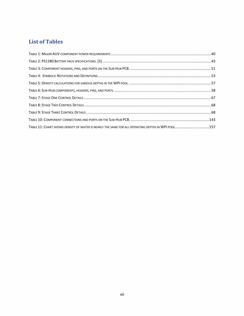
List of Tables

TABLE 1: MAJOR AUV COMPONENT POWER REQUIREMENTS .................................................................................................... 40

TABLE 2: PS1280 BATTERY PACK SPECIFICATIONS. [5] ............................................................................................................ 43

TABLE 3: COMPONENT HEADERS, PINS, AND PORTS ON THE SUB-HUB PCB. ................................................................................. 51

TABLE 4: SYMBOLIC NOTATIONS AND DEFINITIONS ................................................................................................................. 53

TABLE 5: DENSITY CALCULATIONS FOR VARIOUS DEPTHS IN THE WPI POOL. ................................................................................. 57

TABLE 6: SUB-HUB COMPONENTS, HEADERS, PINS, AND PORTS. ................................................................................................ 58

TABLE 7: STAGE ONE CONTROL DETAILS ............................................................................................................................... 67

TABLE 8: STAGE TWO CONTROL DETAILS .............................................................................................................................. 68

TABLE 9: STAGE THREE CONTROL DETAILS ............................................................................................................................ 68

TABLE 10: COMPONENT CONNECTIONS AND PORTS ON THE SUB-HUB PCB. .............................................................................. 143

TABLE 11: CHART SHOWS DENSITY OF WATER IS NEARLY THE SAME FOR ALL OPERATING DEPTHS IN WPI POOL. ................................. 157

1

1 Introduction

The primary objective for the 2009-2010 Autonomous Underwater Vehicle (AUV) Major

Qualifying Project (MQP) was to program, optimize, and complete work on an existing submersible

platform built by the AUV MQP group from the 2008-2009 school year. The efforts of the previous MQP

group yielded a custom manufactured vehicle hull, complete with an internal plumbing system,

stabilizing thrusters, and a primary thruster prototype. A custom made Printed Circuit Board (PCB) was

also manufactured for integrating the AUV’s electronic and software systems. Plans for installing and

programming many of the necessary electronic and sensor systems needed to make the submersible

autonomous were begun during that year as well. The previous group did not manage to bring their

design to full operational or autonomous status. The goal of the current 2009-2010 MQP group was to

finish the necessary manufacturing, optimization, and programming work to make the vehicle fully

operational and achieve autonomous motion.

At the onset of the current project, there were two possible directions to focus the project on. A

first direction would have included working to fabricate a completely new vehicle design prototype,

despite the incomplete state of existing AUV design. The second possible direction for the project, and

the option this MQP group chose to pursue, was to continue efforts aimed at optimizing the existing

vehicle from the 2008-2009 MQP while finishing the electrical and programming work required this

platform fully autonomous. Work on a new vehicle design based on the results of this project is strongly

encouraged for a future MQP group.

After taking time to assess the operational status of the vehicle as it was given to the 2009-2010

MQP, a realistic set of final mission objectives for the AUV to complete was devised. The group’s primary

mission objective is to be able make the vehicle dive (+z-axis) to a specified depth in the WPI pool, move

2

forward in the horizontal direction (+x-axis) for a short distance, and finally rise vertically (-z-axis) to

surface. This mission profile had to be completed autonomously.

When the current group took control of the project, there was a considerable amount of

mechanical and electrical work to be done to complete the objectives of the project. Work that needed

to be done, starting A-Term 2009, included:

• Additional fabrication of hardware components and optimization of components installed

on the vehicle.

• Development of a software programming and control interface.

• Development of a software-based simulation of vehicle dynamics and control schemes.

• Design and fabrication of sensor systems.

• Programming and integration of the control algorithm developed in computer simulations

to the control systems on board the AUV platform.

During the early stages of the project, the group was in close contact with members of the

previous MQP in order to become oriented with the vehicle and its systems. As a result, a large portion

of the group’s effort was also devoted to becoming familiar with the electrical engineering and

programming knowledge that would be needed to complete the vehicle and meet the final mission

objectives.

Much of the early work during the 2009-2010 school year was dedicated to the fabrication of a

new Primary thruster prototype and construction of external mounting brackets for these thrusters.

Additional work was done to integrate a self-contained power source to the vehicle platform and

optimize electronic subsystems for operational use. Finally, vehicle dynamics and control algorithms

were developed in a software simulation written in MATLAB.

3

As work progressed in early 2010, mechanical and electrical subsystem testing was initiated in

the WPI (CAN MUVE) laboratory and in the WPI pool. The results of these tests lead to several full-scale

“wet” tests in the WPI pool, culminating in a final complete systems test where the vehicle performed a

basic motion mission profile autonomously.

4

2 Background Information

Just before sunrise on September 7th, 1776 the “Turtle” crept quiet and unnoticed towards its

intended target, a British ship in the New York harbor. Outfitted with manually driven propellers, this

submerged craft was supposed to drill into the hull of its target, attach a keg of gunpowder with a clock

detonator and escape unnoticed. Although the vehicle failed its objective it was the first use of a

submarine for a military strike [1]. Since the “Turtle’s” historic voyage there have been staggering

advances in submarine technology. We have nuclear powered war machines, research vessels that can

dive to great depths and in recent years, an emergence of autonomously controlled unmanned class of

submersible vehicles.

There are several advantages to operating submersible unmanned Autonomous Underwater

Vehicles (AUV’s). They have the ability to remove human limitations from a mission’s restricting factors.

AUVs can operate at a far greater range of depths and can access environments too dangerous for

human operation. AUV’s are also well suited for long duration missions involving repetitive tasks such as

object-location and wide area patrol. Due to the relatively recent development of Autonomous

Underwater Vehicles, there remains exciting research to be done in the field of autonomous vehicle

control. Many of the concepts involving submersible vehicle dynamics and stability, control theory, and

mechanical system operation remain exciting areas of research. A fully functional AUV system for use by

the WPI Mechanical Engineering Department would provide an exciting test-bed for the research of

hardware and software systems such as navigation units and control algorithms.

Several commercially available AUV systems exist, however they are typically too costly or not

adaptable enough to test a wide-range of various hardware and software systems. So far at WPI, two

previous MQP groups have attempted to build a custom, low-cost AUV from the ground up. The 2008-

5

2009 AUV MQP in particular made significant progress to this end, beginning design and construction of

an autonomous vehicle that would be low cost and highly adaptable.

The sections below describe the major elements commonly found on AUV platforms and also

describe the components that existed on the WPI AUV when the 2009-2010 MQP took control of the

project.

2.1 Vehicle Hull Design

The hull assembly of the vehicle consists of an upper and lower Lexan shell secured together

with a custom developed sealing system. The shells are composed of symmetrically horizontal and

vertical panels; the seams where each panel meets are internally lined with clear silicon sealant and

externally sealed with cyanoacrylate and another layer of silicone sealant. For further assurance, “Grip-

Dip” liquid rubber is painted on the external seams where Lexan pieces meet, to ensure that no leaks

will occur at these joints.

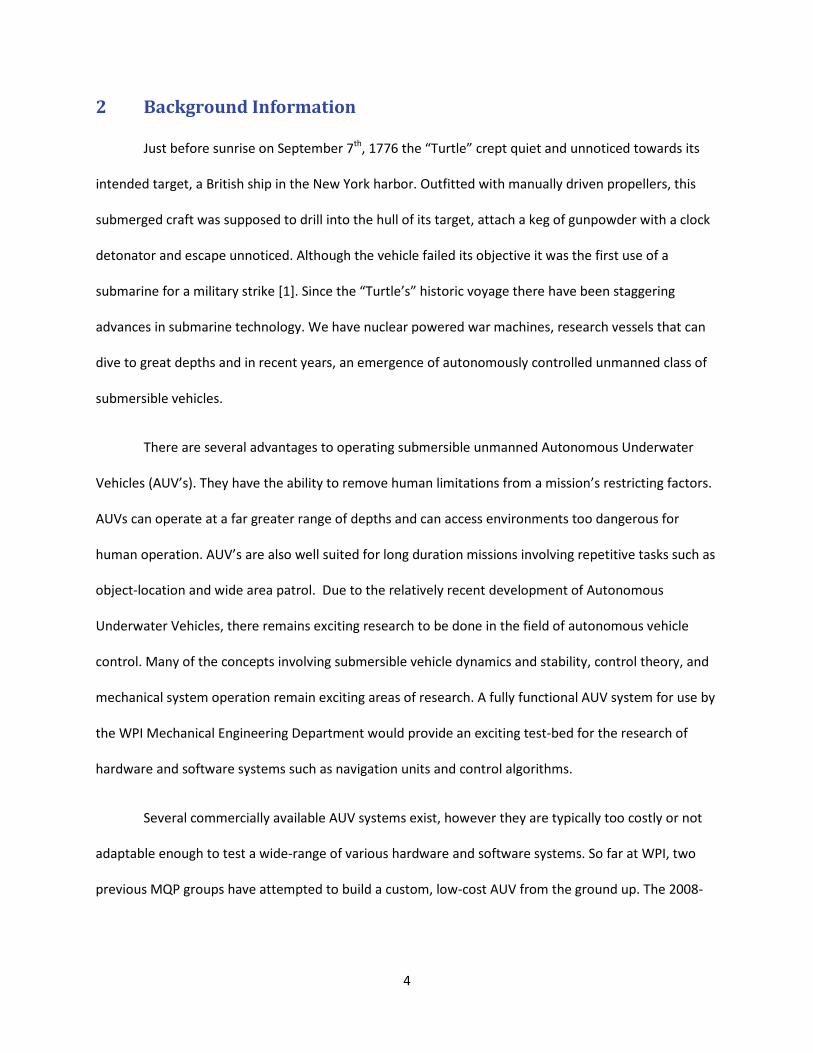
Figure 1: Extruded H-bar diagram with dimensions [2].

Adjoining the two Lexan shells is a rectangular framework made from H-bar aluminum

extrusions as seen in Figure 1. [2] One side of this structure is attached to the lower shell using silicon

sealant; the other is lined with a rubber gasket to form a compression seal with the upper shell.

Petroleum jelly is filled on top of the gasket to maintain and ensure a complete seal. In addition, the

rubber draw latches are used to anchor the shells together and form a waterproof hull.

6

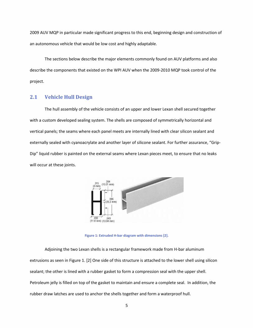
Within the hull is a custom-made aluminum frame that takes form of a rectangular prism. The frame is

press fit on to the lower shell on the hull. It is comprised of detachable beams that will allow future

changes in internal configuration to take place. For further flexibility of component set up and center of

mass calculations, a sliding mount for the pump is present. This frame also provides a system for

electronic components to be mounted and support for the sides of the hull which decreases deflections

and consequently increases the overall strength of the seal. The frame is pictured below in Figure 2. [2]

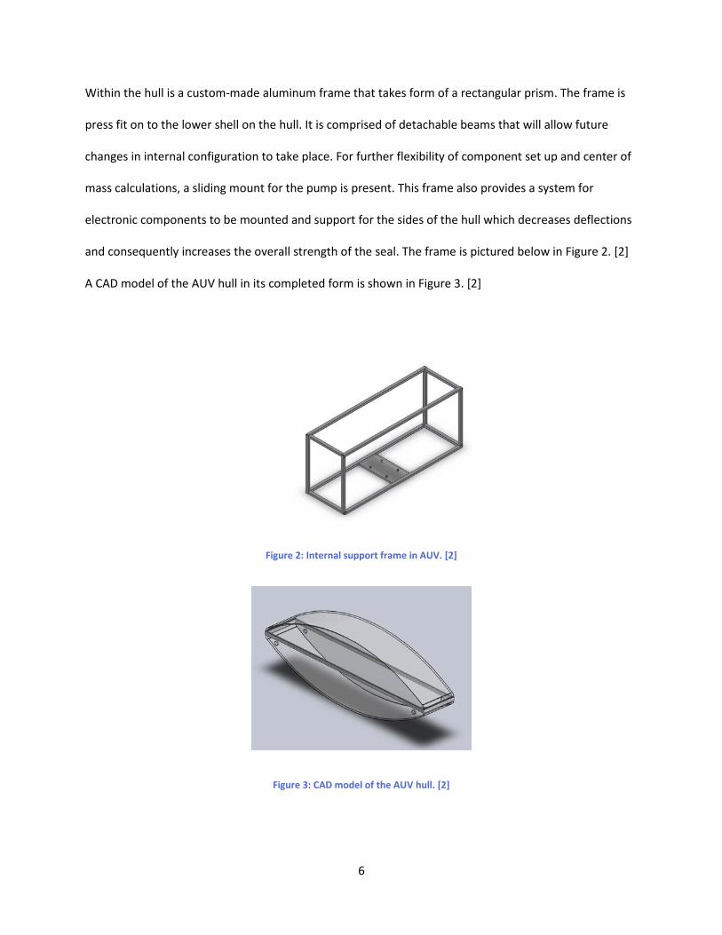
A CAD model of the AUV hull in its completed form is shown in Figure 3. [2]

Figure 2: Internal support frame in AUV. [2]

Figure 3: CAD model of the AUV hull. [2]

7

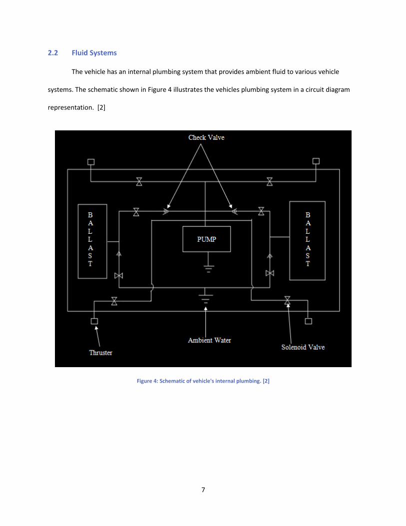
2.2 Fluid Systems

The vehicle has an internal plumbing system that provides ambient fluid to various vehicle

systems. The schematic shown in Figure 4 illustrates the vehicles plumbing system in a circuit diagram

representation. [2]

Figure 4: Schematic of vehicle's internal plumbing. [2]

8

The vehicle pumps ambient fluid from an opening in the bottom of the hull. The water is

pressurized and then travels through a series of clear vinyl tubing connected by plastic “L” and “T”

connectors, sealed with metal clamps and PVC cement.

The majority of the flow is distributed through ½” vinyl tubing and four separate solenoid valves

to four water jet thrusters that control the submarines attitude (pitch and roll). There are also much

smaller bleed lines that connect to the vehicles ballast tanks to allow the vehicle to change its buoyancy

depending on the desired operation. The fluid must travel through a solenoid and check valve on its way

in and out of the ballast tanks. The internal plumbing design is crucial to the vehicle’s operation. Fluid

pumped into the system is pressurized and is in turn used by both the ballast tank system and the four

water-jet nozzles located on the 4 corners of the vehicle.

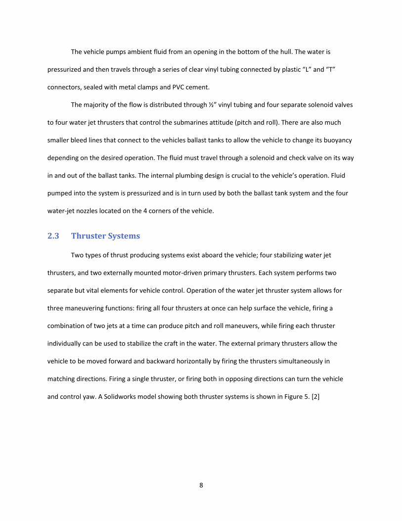
2.3 Thruster Systems

Two types of thrust producing systems exist aboard the vehicle; four stabilizing water jet

thrusters, and two externally mounted motor-driven primary thrusters. Each system performs two

separate but vital elements for vehicle control. Operation of the water jet thruster system allows for

three maneuvering functions: firing all four thrusters at once can help surface the vehicle, firing a

combination of two jets at a time can produce pitch and roll maneuvers, while firing each thruster

individually can be used to stabilize the craft in the water. The external primary thrusters allow the

vehicle to be moved forward and backward horizontally by firing the thrusters simultaneously in

matching directions. Firing a single thruster, or firing both in opposing directions can turn the vehicle

and control yaw. A Solidworks model showing both thruster systems is shown in Figure 5. [2]

9

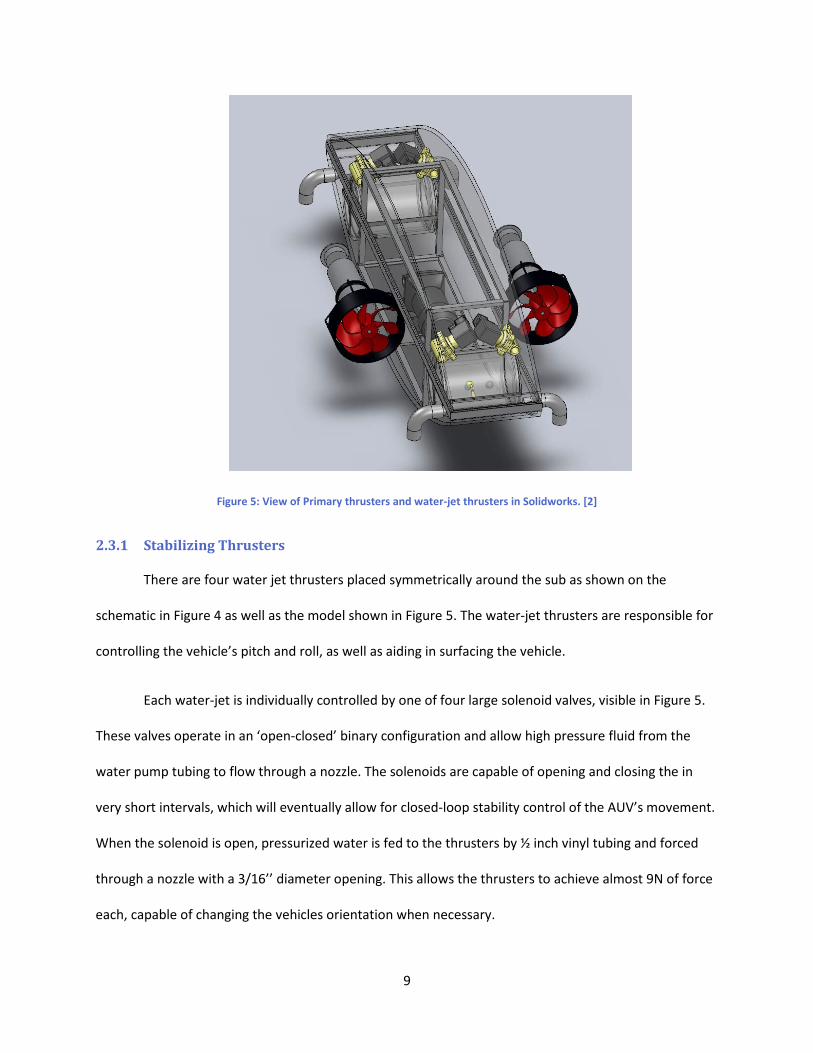
Figure 5: View of Primary thrusters and water-jet thrusters in Solidworks. [2]

2.3.1 Stabilizing Thrusters

There are four water jet thrusters placed symmetrically around the sub as shown on the

schematic in Figure 4 as well as the model shown in Figure 5. The water-jet thrusters are responsible for

controlling the vehicle’s pitch and roll, as well as aiding in surfacing the vehicle.

Each water-jet is individually controlled by one of four large solenoid valves, visible in Figure 5.

These valves operate in an ‘open-closed’ binary configuration and allow high pressure fluid from the

water pump tubing to flow through a nozzle. The solenoids are capable of opening and closing the in

very short intervals, which will eventually allow for closed-loop stability control of the AUV’s movement.

When the solenoid is open, pressurized water is fed to the thrusters by ½ inch vinyl tubing and forced

through a nozzle with a 3/16’’ diameter opening. This allows the thrusters to achieve almost 9N of force

each, capable of changing the vehicles orientation when necessary.

10

2.3.2 Main Thrusters

The vehicles primary propulsion is delivered by motor driven thrusters mounted externally on

the vehicle. The previous MQP group designed and manufactured a prototype thruster that utilizes a

magnetically-driven coupling system. The prototype consists of an aluminum motor housing, two

aluminum end caps, a 12 volt motor that produces 23.69 oz-in of torque and 467 rpm, a rotating internal

magnetic cup, and rotating magnetic shaft connected to a propeller.

The group also discussed a concept for a more compact, lightweight thruster design that would

eliminate all dynamic seals (seals around a moving object) and utilize only static seals. From this idea we

developed and manufactured a second generation of thrusters discussed in methodology.

2.4 Ballast System

An object will float in a fluid if its weight is equal to or less than the weight of the fluid it

displaces. The displacement of fluid creates a force which counteracts gravity’s downward pull. This

resulting force is known as the buoyant force. In the case of a submarine or an underwater vehicle, it is

essential for it to have the ability to sink and surface at will. Hence, a submersible vehicle requires a

means to control its buoyancy in a fluid. The ability to control buoyancy on a submersible craft is most

often achieved through the utilization of a ballast system.

Ballast systems control the flow of fluid in or out of tanks attached to the vehicle, consequently

changing the buoyancy of the system. Changes in vehicle buoyancy allow the vehicle to: ascend (by

pumping water out of tanks or filling tanks with a light gas), descend (filling tanks with water) or remain

steady in a neutral state within the fluid by achieving equilibrium. To allow the vehicle to remain on the

surface of a fluid, or to perform a surfacing maneuver, the ballast tanks are filled with air. This reduces

the overall density of the vehicle, making it lighter than that of the surrounding water. To submerge the

vehicle, the ballast tanks are flooded with water. This process increases the overall density of the

11

vehicle, making it greater than the surrounding water and thus causing it to sink. Once at a desired

depth in the fluid, the vehicle will stabilize. This is executed by maintaining a balance of air and water in

the tanks such that the overall density is equal to the surrounding water. In this state, the system is said

to be neutrally buoyant. Using a combination of tanks placed in strategic positions in the vehicle will also

allow control of vehicle pitch. By setting one end of the submarine to be less dense than the other end,

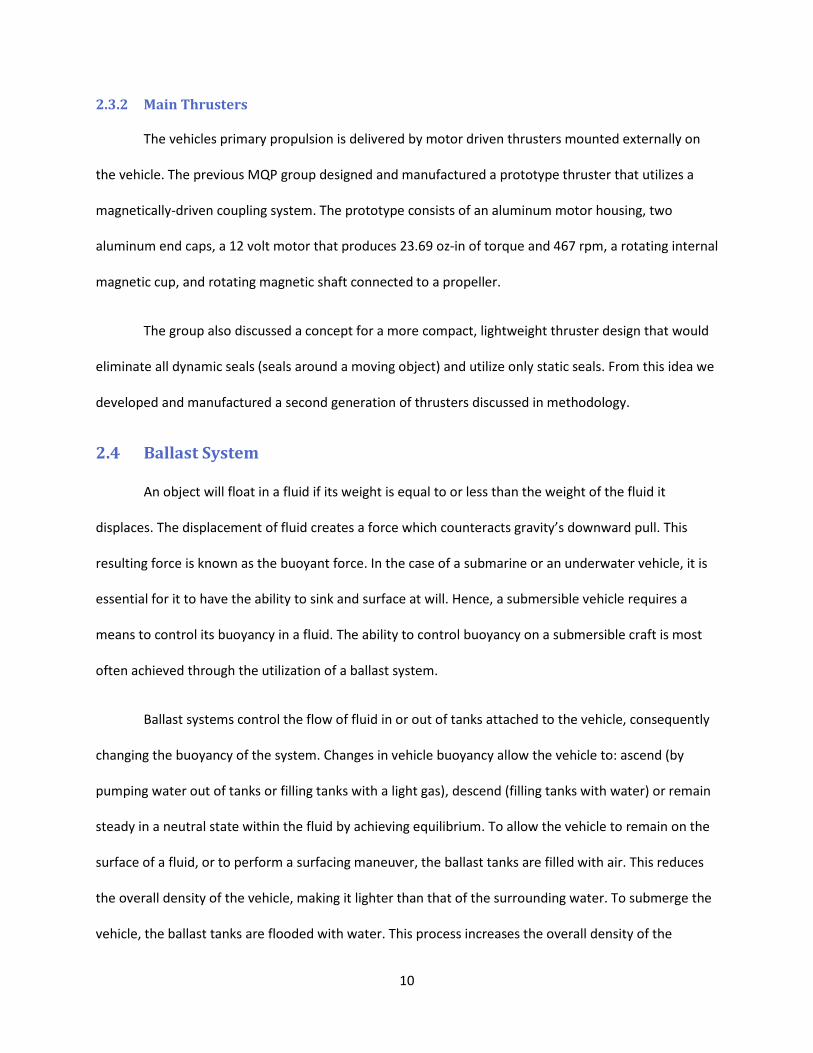
the vehicle will pitch. Figure 6 illustrates each of the cases described above.

Figure 6: Ballast tank effects on vehicle buoyancy. [3]

The ballast system currently in place within the CAN MUVE AUV at WPI uses a system similar to

the one described. The ballast system consists of two air-pressurized ballast tanks positioned in the fore

and aft of the vehicle. Each ballast tank has separate fluid lines to control the filling and evacuation of

fluid. Fluid through these lines is controlled by an ‘open/close’ solenoid valve. For reference of where

bleed lines and solenoids connect from the water pump to the ballast tanks, refer to the fluid systems

schematic shown in Figure 4.

To prevent fluid within the tanks from shifting during maneuvers in the water, possibly

throwing of the AUV’s center of gravity, an expandable latex membrane within each tank helps to keep

12

the fluid stable. The volume of air surrounding the membrane is pressurized to 40 psi through a valve

located on the tank. When filled with fluid, the remaining pressurized air in the tank will act to force

fluid from the latex membrane. When the ‘exit’ solenoid valves leading from each tank are opened, the

ballast tank fluid will be forced from the membrane, through the fluid feed system, and finally expelled

back into the surrounding water from the opening in the hull under the pump. The vehicle is not

designed to operate in depths exceeding those found in the WPI pool (3’-8’), and as such the 40psi back

pressure in each ballast tank is sufficient to overcome and water depth pressure that would impede the

exit of fluid from the ballast system.

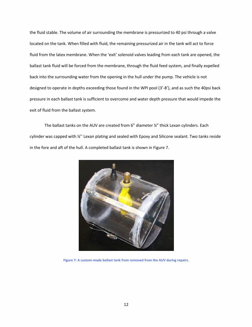
The ballast tanks on the AUV are created from 6” diameter ¼” thick Lexan cylinders. Each

cylinder was capped with ¼’’ Lexan plating and sealed with Epoxy and Silicone sealant. Two tanks reside

in the fore and aft of the hull. A completed ballast tank is shown in Figure 7.

Figure 7: A custom-made ballast tank from removed from the AUV during repairs.

13

2.5 Power System

The power system in an AUV provides the electrical power needed to run the vehicle’s thrusters,

solenoids, electronics, and sensors. The power system must be self-contained within the vehicle to

provide true autonomous capability to the platform. Most autonomous vehicles rely on rechargeable

battery packs to provide the necessary power to all vehicle subsystems.

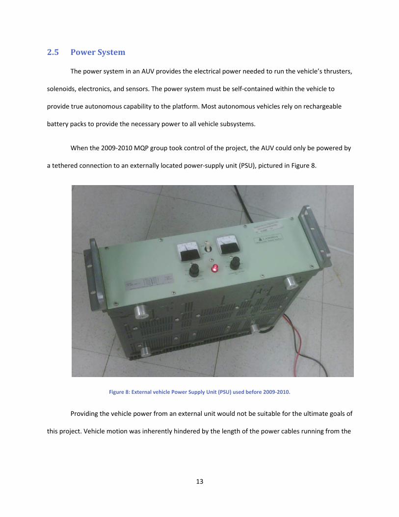
When the 2009-2010 MQP group took control of the project, the AUV could only be powered by

a tethered connection to an externally located power-supply unit (PSU), pictured in Figure 8.

Figure 8: External vehicle Power Supply Unit (PSU) used before 2009-2010.

Providing the vehicle power from an external unit would not be suitable for the ultimate goals of

this project. Vehicle motion was inherently hindered by the length of the power cables running from the

14

PSU located on-shore to the vehicle operating in the water. As described later in this report, a self-

contained, rechargeable, dual-battery pack configuration was chosen to provide power to the vehicle.

In its current configuration the vehicle requires a total of 175 W, with a power draw of 15A (2)

for fully functional operation. This includes power draws from all electronic and mechanical

components, and also accounts for the sensor systems to be added to the vehicle in the future. The

initial Estimated Time of vehicle Operation (ETO) (including preparation, calibration, testing) was 30

minutes, as given by the previous MQP group. This ETO meant that the minimum needed power

capacity of the Power System would be 87.5Wh. These specifications would provide the basis for the

selection of a suitable power supply for the current MQP group.

2.6 Electronics

The submarine’s various electronic systems and subsystems must function together to monitor

and control all aspects of the vehicle’s operation. The primary electronics systems on the submarine

include the Central Processing Unit (CPU), Sub-Hub interface, Sensors, and Actuators. These systems

must work cohesively to provide control of the mechanical components of the vehicle. Many of the

components described in this section were bought during the previous year and were on hand during

the beginning of the 2009-2010 year. Other components were later purchased by the current MQP

group. At the start of the 2009-2010 school year, none of the electronic components of the vehicle were

installed or programmed in order to achieve autonomous motion. Construction of the AUV’s electronics

systems are described later in Section 3 Methodology.

Efforts from the previous 2008-2009 MQP group had mapped out many aspects of the system

dynamics and component design needed to complete the electronic systems in the existing vehicle.

Vehicle operation would be controlled by interactions between three main system groups; central

processing (PC/104 stack), sensor/actuator Interface (Sub-Hub PCB with MSP430 chip), and sensor

15

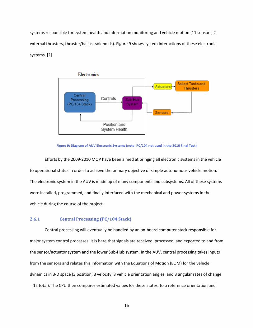
systems responsible for system health and information monitoring and vehicle motion (11 sensors, 2

external thrusters, thruster/ballast solenoids). Figure 9 shows system interactions of these electronic

systems. [2]

Figure 9: Diagram of AUV Electronic Systems (note: PC/104 not used in the 2010 Final Test)

Efforts by the 2009-2010 MQP have been aimed at bringing all electronic systems in the vehicle

to operational status in order to achieve the primary objective of simple autonomous vehicle motion.

The electronic system in the AUV is made up of many components and subsystems. All of these systems

were installed, programmed, and finally interfaced with the mechanical and power systems in the

vehicle during the course of the project.

2.6.1 Central Processing (PC/104 Stack)

Central processing will eventually be handled by an on-board computer stack responsible for

major system control processes. It is here that signals are received, processed, and exported to and from

the sensor/actuator system and the lower Sub-Hub system. In the AUV, central processing takes inputs

from the sensors and relates this information with the Equations of Motion (EOM) for the vehicle

dynamics in 3-D space (3 position, 3 velocity, 3 vehicle orientation angles, and 3 angular rates of change

= 12 total). The CPU then compares estimated values for these states, to a reference orientation and

16

reference path. Based on the result of these operations, signals are output to the Sub-Hub system and

then finally to the actuators (solenoids controlling thrusters and ballasts) to correct the trajectory of the

vehicle as needed.

A full vehicle motion simulation was written in MATLAB (Refer to Appendix A: MATLAB Code).

This simulation program must later be integrated into a language that the PC/104 system can

understand. The primary objective of the Central Processing system (and Electronics systems as a whole)

in relation to the goals of the project is to guide the craft to an objectified position efficiently and safely.

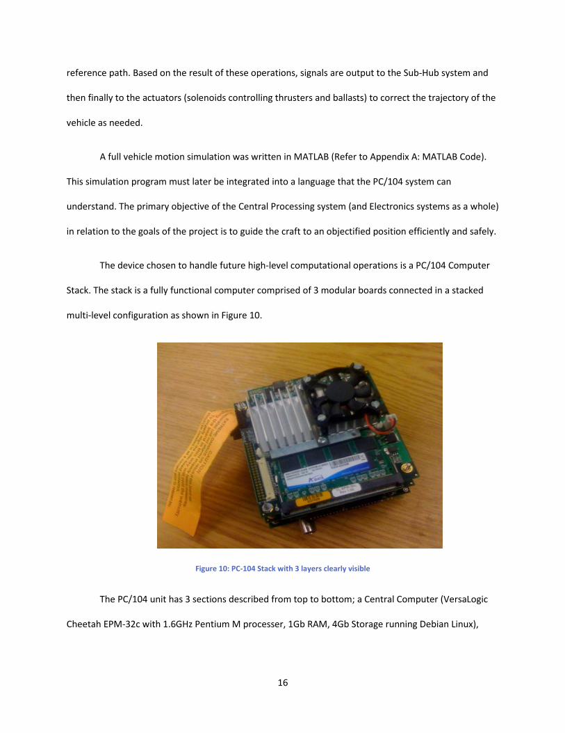
The device chosen to handle future high-level computational operations is a PC/104 Computer

Stack. The stack is a fully functional computer comprised of 3 modular boards connected in a stacked

multi-level configuration as shown in Figure 10.

Figure 10: PC-104 Stack with 3 layers clearly visible

The PC/104 unit has 3 sections described from top to bottom; a Central Computer (VersaLogic

Cheetah EPM-32c with 1.6GHz Pentium M processer, 1Gb RAM, 4Gb Storage running Debian Linux),

17

Frame Grabber unit (Sensoray Model 311), and an Analog to Digital Convertor unit (VersaLogic VCM-

DAS-1 “Data Acquisition and Control Module”).

The component had been purchased by the 2008-2009 group, but was not programmed to

control and take readings from the sensor and actuator systems. The processing power of the PC/104

stack was not required for the basic autonomously controlled motion profile that was the primary object

of the current project. For the purposes of the 2009-2010 MQP, control of the AUV was handled solely

by the MSP430 Sub-Hub PCB, described in the following section. In future mission profiles of greater

complexity, especially those requiring additional sensor systems and multiple mission objectives, the

PC/104 Stack will be necessary to provide the necessary computing power.

2.6.2 MSP430 Sub-Hub System

The MSP430 Sub-Hub PCB, or Sub-Hub system, is comprised of a WPI-built Printed Circuit Board

(PCB) controlled by a MSP-430-F223 microcontroller chip. The entire Sub-Hub system resides on a

custom-designed PCB designed at WPI. The Sub-Hub board also provides an I/O interface for the control

of the external thrusters, solenoids, and basic sensor systems. The Sub-Hub MSP-430 also facilitates

basic data processing, as was utilized by this project and described later in Section 3 Methodology.

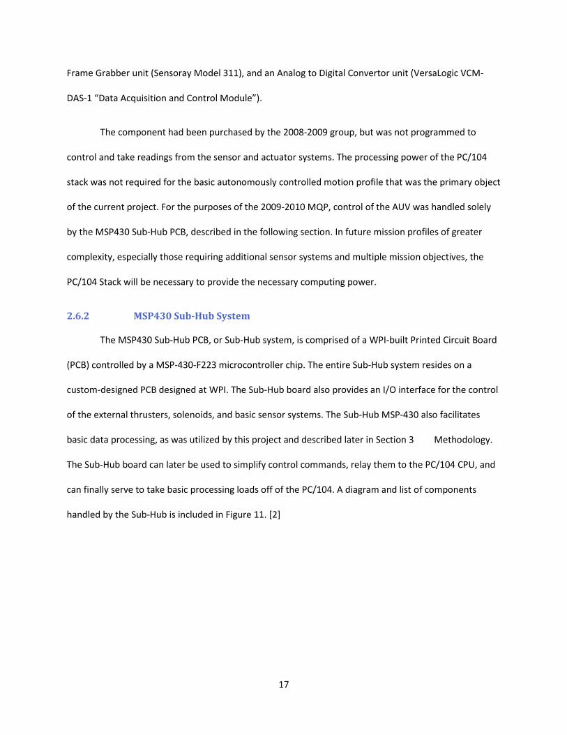
The Sub-Hub board can later be used to simplify control commands, relay them to the PC/104 CPU, and

can finally serve to take basic processing loads off of the PC/104. A diagram and list of components

handled by the Sub-Hub is included in Figure 11. [2]

18

Figure 11: Diagram of Sub-Hub system and interactions. [2]

The Sub-Hub interface has the capability to receive commands from a multitude of electronic

components and sensor systems on the AUV. A list of the systems which the Sub-Hub PCB may control is

included in the list below. [2]

• Emergency ballast solenoid driver, 1

• Pump Driver, 1

• Main thruster motor driver, 2

• On-board temperature sensor (Cabin Temperature), 1

• Remote temperature sensor (PC104 Temperature), 1

• 1.25V reference generator, 1

• Pressure sensor, 3

• Supply Voltage Monitor, 1

• Water leak sensor, 1

• I2C bus lines and pull-up resistors, 1

• SPI bus lines, 1

• MSP430 circuitry

19

High frequency crystal oscillator (for MSP430), 1

Low frequency crystal oscillator (for MSP430), 1

JTAG programming interface (for MSP430), 1

• Power connections, 1x3.3V, 1x5V, 4x12V

The capabilities of the Sub-Hub PCB were deemed sufficient to meet the computing, processing,

and interfacing need of this project. As such, the PC/104 computing stack was not used to achieve this

MQP’s basic motion profile. More complex mission profiles in future iterations of this AUV system

should use the Sub-Hub PCB interface for basic sensor and actuator control, while complex control

algorithms are run externally from the PC/104 stack.

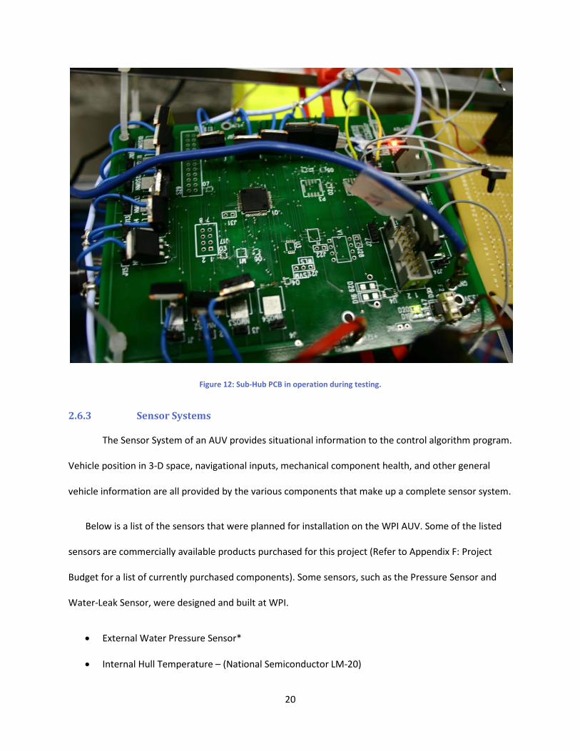
Figure 12 shows a photograph of the completed Sub-Hub PCB in operation. The MSP-430

processing chip can be seen located in the center of the board.

20

Figure 12: Sub-Hub PCB in operation during testing.

2.6.3 Sensor Systems

The Sensor System of an AUV provides situational information to the control algorithm program.

Vehicle position in 3-D space, navigational inputs, mechanical component health, and other general

vehicle information are all provided by the various components that make up a complete sensor system.

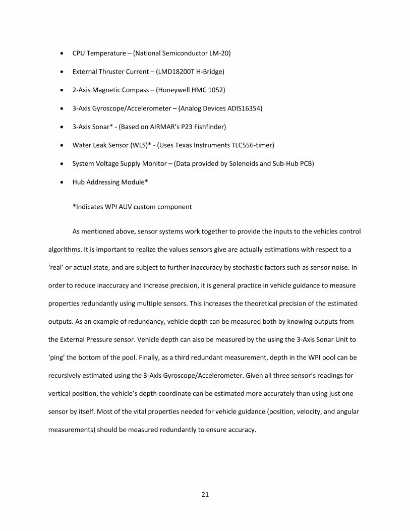
Below is a list of the sensors that were planned for installation on the WPI AUV. Some of the listed

sensors are commercially available products purchased for this project (Refer to Appendix F: Project

Budget for a list of currently purchased components). Some sensors, such as the Pressure Sensor and

Water-Leak Sensor, were designed and built at WPI.

• External Water Pressure Sensor*

• Internal Hull Temperature – (National Semiconductor LM-20)

21

• CPU Temperature – (National Semiconductor LM-20)

• External Thruster Current – (LMD18200T H-Bridge)

• 2-Axis Magnetic Compass – (Honeywell HMC 1052)

• 3-Axis Gyroscope/Accelerometer – (Analog Devices ADIS16354)

• 3-Axis Sonar* - (Based on AIRMAR’s P23 Fishfinder)

• Water Leak Sensor (WLS)* - (Uses Texas Instruments TLC556-timer)

• System Voltage Supply Monitor – (Data provided by Solenoids and Sub-Hub PCB)

• Hub Addressing Module*

*Indicates WPI AUV custom component

As mentioned above, sensor systems work together to provide the inputs to the vehicles control

algorithms. It is important to realize the values sensors give are actually estimations with respect to a

‘real’ or actual state, and are subject to further inaccuracy by stochastic factors such as sensor noise. In

order to reduce inaccuracy and increase precision, it is general practice in vehicle guidance to measure

properties redundantly using multiple sensors. This increases the theoretical precision of the estimated

outputs. As an example of redundancy, vehicle depth can be measured both by knowing outputs from

the External Pressure sensor. Vehicle depth can also be measured by the using the 3-Axis Sonar Unit to

‘ping’ the bottom of the pool. Finally, as a third redundant measurement, depth in the WPI pool can be

recursively estimated using the 3-Axis Gyroscope/Accelerometer. Given all three sensor’s readings for

vertical position, the vehicle’s depth coordinate can be estimated more accurately than using just one

sensor by itself. Most of the vital properties needed for vehicle guidance (position, velocity, and angular

measurements) should be measured redundantly to ensure accuracy.

22

2.6.3.1 Sensor System Integration

Some of the components listed in Section 2.6.3 require little more than basic interfacing and

calibration with the Sub-Hub system in order for useful operation. The 3-axis gyroscope/accelerometer,

voltage monitors, temperature sensors, and the 2-axis magnetic compass are pre-assembled,

commercially purchased units that interface to ports on the Sub-Hub system or directly to the Central

Processing PC/104 stack. Sensors such as the 3-axis sonar unit, external water pressure sensor, and

water leak sensor were designed custom to the needs of this project by both the 2008-2009 MQP and

the current 2009-2010 MQP groups and will require custom developed means for calibration.

2.7 AUV Control Algorithms

A means of controlling an AUV’s motion within the water must be handled by a control

algorithm programmed and run on the CPU. The concept of an AUV control algorithm is nearly identical

to those found in manned and unmanned aircraft control systems, the most notable difference being

the medium through which the vehicles move. A control algorithm must account for the AUV’s motions

and dynamics while moving through a fluid in 3 dimensions. The program should take environmental

inputs from the sensor system and output necessary commands to the vehicle’s motion controlling

components (pitch, roll, yaw, thrust).

Control algorithms are typically categorized into two types in control theory: open-loop and

closed-loop controllers. Open-loop controllers simply output commands to the system without taking

into account the effect of destabilizing forces that the vehicle may encounter. They assume ideal

operating conditions within the environment. For example, an open-loop controller in an AUV would not

take into account disturbances in pressure and density while the vehicle moves through the water. The

WPI AUV as tested in during the current project exhibits an autonomous open-loop scheme.

23

Closed-loop controllers account for small disturbances to the vehicle’s motion and orientation in

an environment. These controllers implement feed-back loops which continuously take in

measurements from sensor systems about the vehicle’s orientation and position in 3-D space. The

controller will then make the necessary adjustments to keep the vehicle on a desired course while

keeping control errors to a minimum. Future work with the WPI AUV will allow for closed-loop control.

More detailed information regarding the control algorithms and programs used by this MQP can be

found in section 3.7 Vehicle Control Algorithms and Simulation.

24

3 Methodology

At the beginning of this MQP, the group worked to familiarize itself with all of the work the

previous group completed or started for the AUV. As described, the vehicle had a completed hull,

internal fluid feed system, stabilizing thrusters, and ballast tanks. Completed as well was a main thruster

prototype. Finally, only basic electronic and sensor designs were developed, while no sensor, electronic,

or power systems were integrated into the vehicle. There was a large amount of work left to complete

to produce an operational vehicle and achieve autonomous motion in the WPI pool.

The group began work by ensuring the AUV hull design was acceptable and was sealed properly.

Next, the group began testing and fixing design problems with the original fluid feed systems.

Simultaneously, the group began designing, manufacturing, and testing a new Primary thruster system;

requiring a new propeller, Primary thruster bracket, and a new propeller cowl design. As design and

hardware optimization was completed, work began on integrating an internal power supply and

configuring all necessary electronic systems on the vehicle. Throughout the course of the project,

vehicle control algorithms and programming methods were explored. These efforts produced a fully

functional MATLAB simulation of the vehicle’s motion maneuvers, later used to help program the sub to

complete a basic motion profile in the WPI pool. The following subsections discuss the work done on

each of the areas mentioned.

25

3.1 Hull

The hull of the vehicle houses all the electronics and sensitive components. It was imperative for

“wet” testing that the hull was sealed properly. The vehicle was sealed by filling the channel in the

bottom half of the hull with petroleum jelly and then closing the top half on the hull in the petroleum

and clamping it down with rubber clasps. The corners of the hull are coated with a black gasket caulking

and all holes in the hull are sealed with silicone caulk.

3.2 Fluid Systems

After meeting with the previous group the current MQP group was warned of a problem with

internal leakage in the vehicle’s fluid-feed system at the interfaces of the vinyl tubing and metal clamps.

The project’s first goal was to resolve these issues, since the hull contains expensive and vital electronic

components that would potentially be destroyed by a leak in the internal plumbing system. The vehicle’s

plumbing was inspected and it was discovered that several fluid-feed clamps were missing. The missing

clamps were installed and tightened to insure proper sealing.

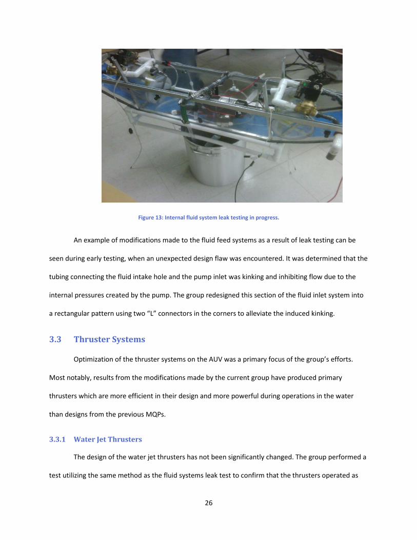
3.2.1 Leak Checking

A simple leak test was implemented to verify that the internal leaking in the fluid feed system

was no longer occurring. The test can be seen in Figure 13. The vehicle was placed over a bucket of

water and a hose was attached to the hole in the bottom of the hull where the water takes in

surrounding fluid. Several tests in a similar configuration to the one shown were conducted to quickly

check modifications made to the fluid feed system and to check for leaks during the course of the

project.

26

Figure 13: Internal fluid system leak testing in progress.

An example of modifications made to the fluid feed systems as a result of leak testing can be

seen during early testing, when an unexpected design flaw was encountered. It was determined that the

tubing connecting the fluid intake hole and the pump inlet was kinking and inhibiting flow due to the

internal pressures created by the pump. The group redesigned this section of the fluid inlet system into

a rectangular pattern using two “L” connectors in the corners to alleviate the induced kinking.

3.3 Thruster Systems

Optimization of the thruster systems on the AUV was a primary focus of the group’s efforts.

Most notably, results from the modifications made by the current group have produced primary

thrusters which are more efficient in their design and more powerful during operations in the water

than designs from the previous MQPs.

3.3.1 Water Jet Thrusters

The design of the water jet thrusters has not been significantly changed. The group performed a

test utilizing the same method as the fluid systems leak test to confirm that the thrusters operated as

27

designed. As expected, the thrusters produced a small diameter, high velocity jet of water. The thrusters

are constructed from multiple sections of PVC piping. During the first test this piping disengaged from

another section. This was fixed by applying PVC cement to all the sections. A second test confirmed that

the problem was fixed. All four water-jet thrusters operated successfully during the final mission test.

3.3.2 Primary External Thrusters

As previously stated in Section 2.3.2 Main Thrusters, the previous group had developed a first

generation prototype thruster. After inspecting the prototype and the alternative concept discussed it

was decided to implement a design that would decrease the mass of the thruster, provide smoother

propulsion and eliminate the use of failure-prone dynamic seals. These thrusters, when at their peak

performance, can produce about 13 N of force each.

3.3.2.1 Motor Housing

The motor housing was machined from 3’’ diameter cylindrical aluminum stock. The original

thruster prototype housing had a length of 8.5’’ and an outside diameter of 3’’ (only a small clean cut

was taken off the outside). The housing was symmetrical with a hole in the middle of the tube for the

motor and two larger holes on each end for the magnetic coupling and end caps.

The second generation design utilized a smaller motor housing than the prototype. The new

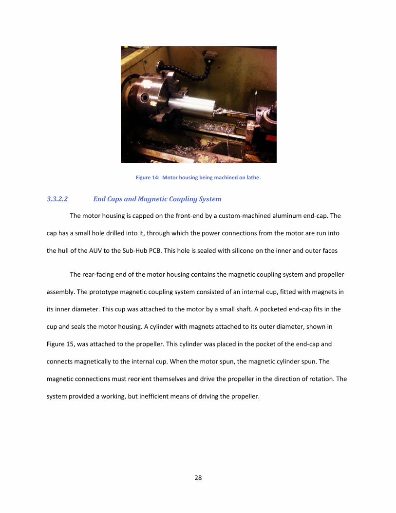
motor housing is 6.5’’ long with an outer diameter of 2.5 ‘’. Shown in Figure 14, the new motor housing

was machined on campus at WPI using a manual lathe.

28

Figure 14: Motor housing being machined on lathe.

3.3.2.2 End Caps and Magnetic Coupling System

The motor housing is capped on the front-end by a custom-machined aluminum end-cap. The

cap has a small hole drilled into it, through which the power connections from the motor are run into

the hull of the AUV to the Sub-Hub PCB. This hole is sealed with silicone on the inner and outer faces

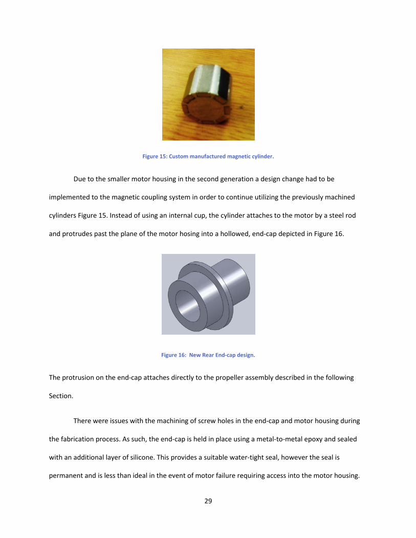
The rear-facing end of the motor housing contains the magnetic coupling system and propeller

assembly. The prototype magnetic coupling system consisted of an internal cup, fitted with magnets in

its inner diameter. This cup was attached to the motor by a small shaft. A pocketed end-cap fits in the

cup and seals the motor housing. A cylinder with magnets attached to its outer diameter, shown in

Figure 15, was attached to the propeller. This cylinder was placed in the pocket of the end-cap and

connects magnetically to the internal cup. When the motor spun, the magnetic cylinder spun. The

magnetic connections must reorient themselves and drive the propeller in the direction of rotation. The

system provided a working, but inefficient means of driving the propeller.

29

Figure 15: Custom manufactured magnetic cylinder.

Due to the smaller motor housing in the second generation a design change had to be

implemented to the magnetic coupling system in order to continue utilizing the previously machined

cylinders Figure 15. Instead of using an internal cup, the cylinder attaches to the motor by a steel rod

and protrudes past the plane of the motor hosing into a hollowed, end-cap depicted in Figure 16.

Figure 16: New Rear End-cap design.

The protrusion on the end-cap attaches directly to the propeller assembly described in the following

Section.

There were issues with the machining of screw holes in the end-cap and motor housing during

the fabrication process. As such, the end-cap is held in place using a metal-to-metal epoxy and sealed

with an additional layer of silicone. This provides a suitable water-tight seal, however the seal is

permanent and is less than ideal in the event of motor failure requiring access into the motor housing.

30

Future groups may wish to improve upon this design, as described in Section 6 Future Work and

Recommendations.

3.3.2.3 Propeller Assembly

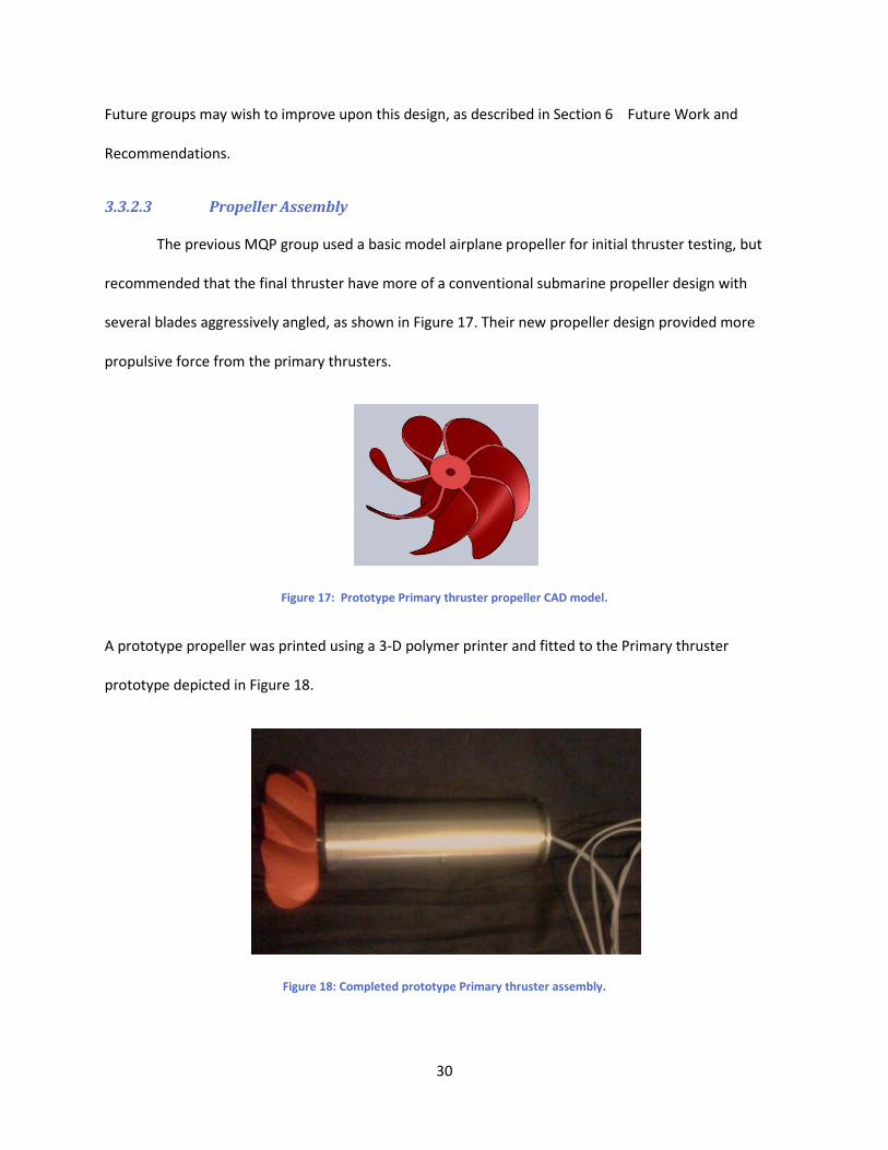
The previous MQP group used a basic model airplane propeller for initial thruster testing, but

recommended that the final thruster have more of a conventional submarine propeller design with

several blades aggressively angled, as shown in Figure 17. Their new propeller design provided more

propulsive force from the primary thrusters.

Figure 17: Prototype Primary thruster propeller CAD model.

A prototype propeller was printed using a 3-D polymer printer and fitted to the Primary thruster

prototype depicted in Figure 18.

Figure 18: Completed prototype Primary thruster assembly.

31

The propeller for the primary thrusters was initially going to remain largely the same as the

prototype developed by the previous MQP group. The current group initially made a slight adjustment

to the angle on the propeller blades, and was able to smooth the edges of the design, thus providing a

less disturbed flow across the blades.

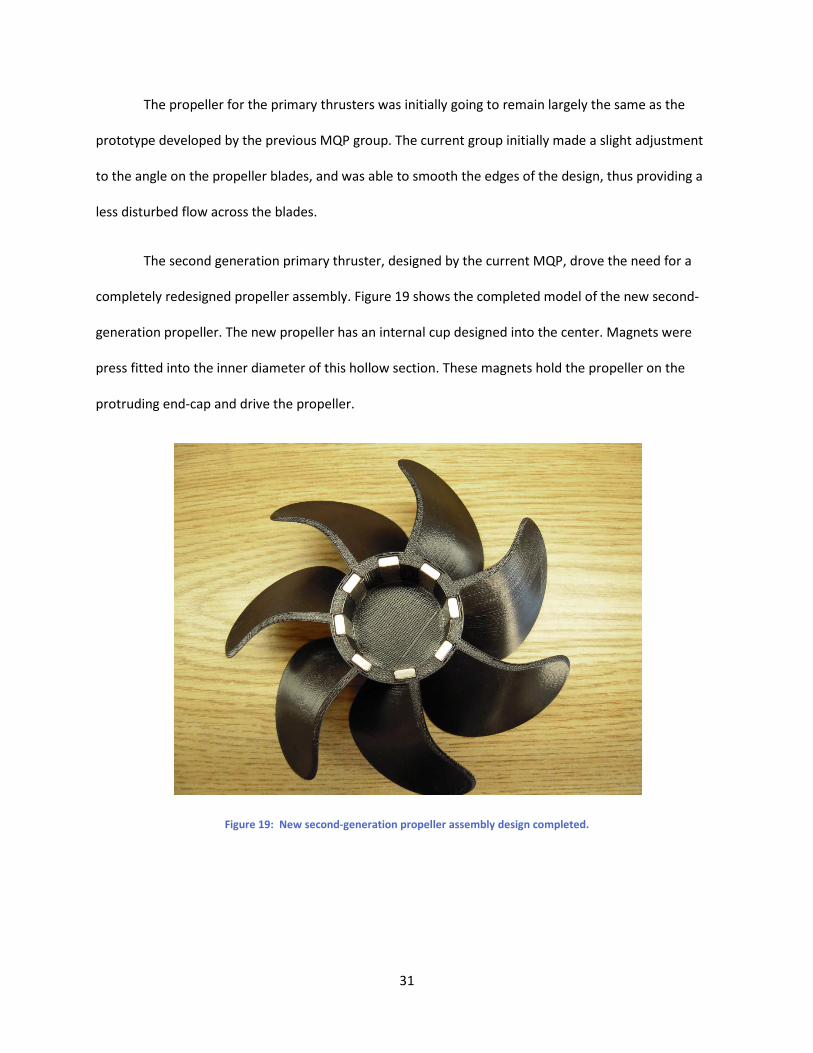
The second generation primary thruster, designed by the current MQP, drove the need for a

completely redesigned propeller assembly. Figure 19 shows the completed model of the new second-

generation propeller. The new propeller has an internal cup designed into the center. Magnets were

press fitted into the inner diameter of this hollow section. These magnets hold the propeller on the

protruding end-cap and drive the propeller.

Figure 19: New second-generation propeller assembly design completed.

32

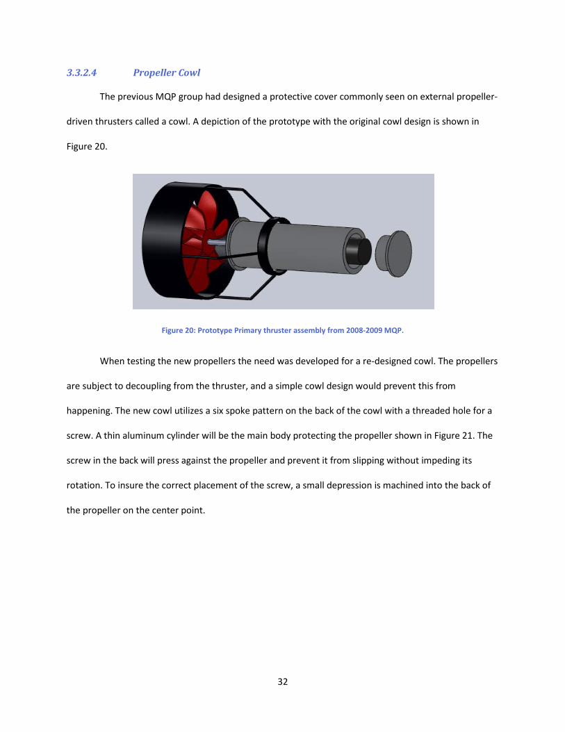
3.3.2.4 Propeller Cowl

The previous MQP group had designed a protective cover commonly seen on external propeller-

driven thrusters called a cowl. A depiction of the prototype with the original cowl design is shown in

Figure 20.

Figure 20: Prototype Primary thruster assembly from 2008-2009 MQP.

When testing the new propellers the need was developed for a re-designed cowl. The propellers

are subject to decoupling from the thruster, and a simple cowl design would prevent this from

happening. The new cowl utilizes a six spoke pattern on the back of the cowl with a threaded hole for a

screw. A thin aluminum cylinder will be the main body protecting the propeller shown in Figure 21. The

screw in the back will press against the propeller and prevent it from slipping without impeding its

rotation. To insure the correct placement of the screw, a small depression is machined into the back of

the propeller on the center point.

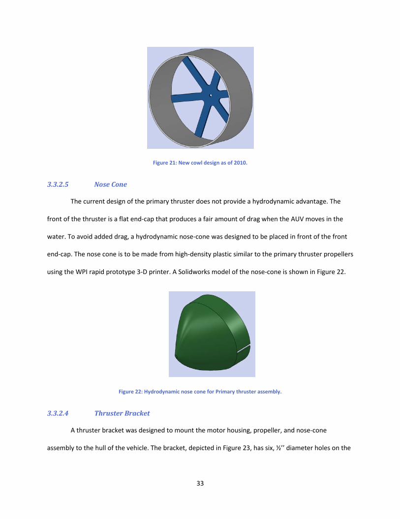
33

Figure 21: New cowl design as of 2010.

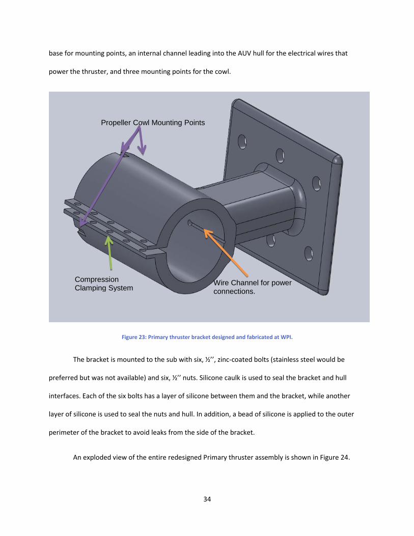
3.3.2.5 Nose Cone

The current design of the primary thruster does not provide a hydrodynamic advantage. The

front of the thruster is a flat end-cap that produces a fair amount of drag when the AUV moves in the

water. To avoid added drag, a hydrodynamic nose-cone was designed to be placed in front of the front

end-cap. The nose cone is to be made from high-density plastic similar to the primary thruster propellers

using the WPI rapid prototype 3-D printer. A Solidworks model of the nose-cone is shown in Figure 22.

Figure 22: Hydrodynamic nose cone for Primary thruster assembly.

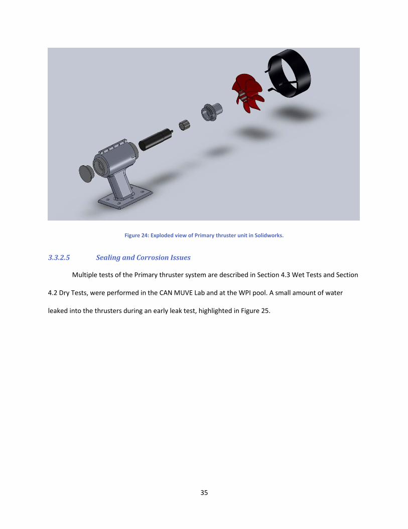
3.3.2.4 Thruster Bracket

A thruster bracket was designed to mount the motor housing, propeller, and nose-cone

assembly to the hull of the vehicle. The bracket, depicted in Figure 23, has six, ½’’ diameter holes on the

34

base for mounting points, an internal channel leading into the AUV hull for the electrical wires that

power the thruster, and three mounting points for the cowl.

Figure 23: Primary thruster bracket designed and fabricated at WPI.

The bracket is mounted to the sub with six, ½’’, zinc-coated bolts (stainless steel would be

preferred but was not available) and six, ½’’ nuts. Silicone caulk is used to seal the bracket and hull

interfaces. Each of the six bolts has a layer of silicone between them and the bracket, while another

layer of silicone is used to seal the nuts and hull. In addition, a bead of silicone is applied to the outer

perimeter of the bracket to avoid leaks from the side of the bracket.

An exploded view of the entire redesigned Primary thruster assembly is shown in Figure 24.

Wire Channel for power connections.

Propeller Cowl Mounting Points

Compression Clamping System

35

Figure 24: Exploded view of Primary thruster unit in Solidworks.

3.3.2.5 Sealing and Corrosion Issues

Multiple tests of the Primary thruster system are described in Section 4.3 Wet Tests and Section

4.2 Dry Tests, were performed in the CAN MUVE Lab and at the WPI pool. A small amount of water

leaked into the thrusters during an early leak test, highlighted in Figure 25.

36

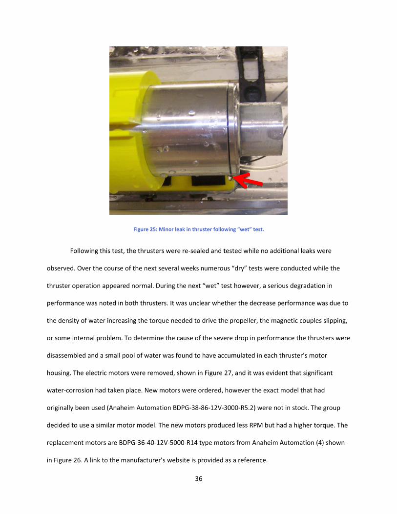
Figure 25: Minor leak in thruster following “wet” test.

Following this test, the thrusters were re-sealed and tested while no additional leaks were

observed. Over the course of the next several weeks numerous “dry” tests were conducted while the

thruster operation appeared normal. During the next “wet” test however, a serious degradation in

performance was noted in both thrusters. It was unclear whether the decrease performance was due to

the density of water increasing the torque needed to drive the propeller, the magnetic couples slipping,

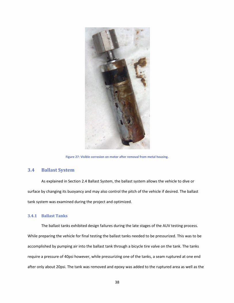
or some internal problem. To determine the cause of the severe drop in performance the thrusters were

disassembled and a small pool of water was found to have accumulated in each thruster’s motor

housing. The electric motors were removed, shown in Figure 27, and it was evident that significant

water-corrosion had taken place. New motors were ordered, however the exact model that had

originally been used (Anaheim Automation BDPG-38-86-12V-3000-R5.2) were not in stock. The group

decided to use a similar motor model. The new motors produced less RPM but had a higher torque. The

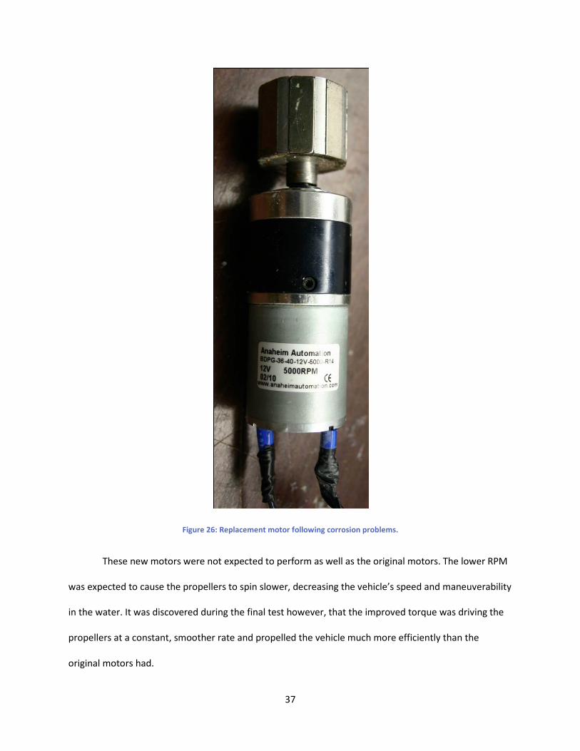
replacement motors are BDPG-36-40-12V-5000-R14 type motors from Anaheim Automation (4) shown

in Figure 26. A link to the manufacturer’s website is provided as a reference.

37

Figure 26: Replacement motor following corrosion problems.

These new motors were not expected to perform as well as the original motors. The lower RPM

was expected to cause the propellers to spin slower, decreasing the vehicle’s speed and maneuverability

in the water. It was discovered during the final test however, that the improved torque was driving the

propellers at a constant, smoother rate and propelled the vehicle much more efficiently than the

original motors had.

38

Figure 27: Visible corrosion on motor after removal from metal housing.

3.4 Ballast System

As explained in Section 2.4 Ballast System, the ballast system allows the vehicle to dive or

surface by changing its buoyancy and may also control the pitch of the vehicle if desired. The ballast

tank system was examined during the project and optimized.

3.4.1 Ballast Tanks

The ballast tanks exhibited design failures during the late stages of the AUV testing process.

While preparing the vehicle for final testing the ballast tanks needed to be pressurized. This was to be

accomplished by pumping air into the ballast tank through a bicycle tire valve on the tank. The tanks

require a pressure of 40psi however, while pressurizing one of the tanks, a seam ruptured at one end

after only about 20psi. The tank was removed and epoxy was added to the ruptured area as well as the

39

seams on the entire tank. In addition, silicone was added to the seams to add an extra degree of leak

protection. Both sections of strapping were reattached to the tank and tightened to help the tank hold

the pressure.

3.4.2 Lead Ballast Weights

In addition to the ballast tanks, extra ballast weight was necessary to achieve neutral to near-

negative buoyancy of the vehicle while in the water. The large volume of air inside the vehicle required

that nearly 125lbs of additional ballast weight was required to achieve negative buoyancy. Some ballast

weight is provided inherently from the weight of the mechanical components, electronics, and batteries

in the hull. Despite this, a majority of the additional ballast weight is provided by custom-made ballasts.

Lead-shot was ordered to provide an additional 95lbs of weight to the AUV. The lead is similar to that

used in SCUBA diving weights.

In order to keep the vehicle balanced with all the additional ballast, various methods of

distributing the weight evenly throughout the sub were developed. The group initially cut eight sections

of 1’’ diameter vinyl tubing (approximately 15’’ long), filled them with the lead shot, and capped each

end to avoid leaking. These tube-weights are lined evenly on both sides of the sub and account for about

15 lbs of the ballast weight.

Some of the additional lead shot was poured into four Latex balloons. Each balloon holds

approximately 5 lbs of shot. Two balloons were placed in the front and two in the rear of the vehicle.

The remaining 50 lbs of ballast comes from two 25 lb cloth bags of lead shot. One is placed in front of

the water pump, while the other is laid on top of the water pump. All together this adds about 95 lbs of

weight just for ballast. All three methods of containing the lead weight are shown in Figure 28.

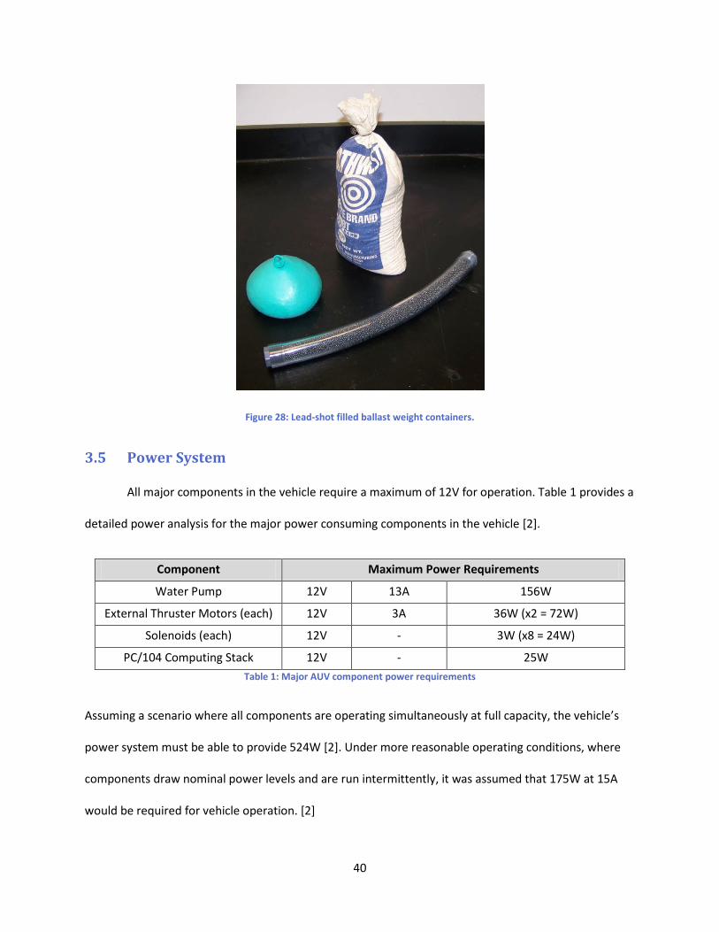
40

Figure 28: Lead-shot filled ballast weight containers.

3.5 Power System

All major components in the vehicle require a maximum of 12V for operation. Table 1 provides a

detailed power analysis for the major power consuming components in the vehicle [2].

Component Maximum Power Requirements

Water Pump 12V 13A 156W

External Thruster Motors (each) 12V 3A 36W (x2 = 72W)

Solenoids (each) 12V - 3W (x8 = 24W)

PC/104 Computing Stack 12V - 25W Table 1: Major AUV component power requirements

Assuming a scenario where all components are operating simultaneously at full capacity, the vehicle’s

power system must be able to provide 524W [2]. Under more reasonable operating conditions, where

components draw nominal power levels and are run intermittently, it was assumed that 175W at 15A

would be required for vehicle operation. [2]

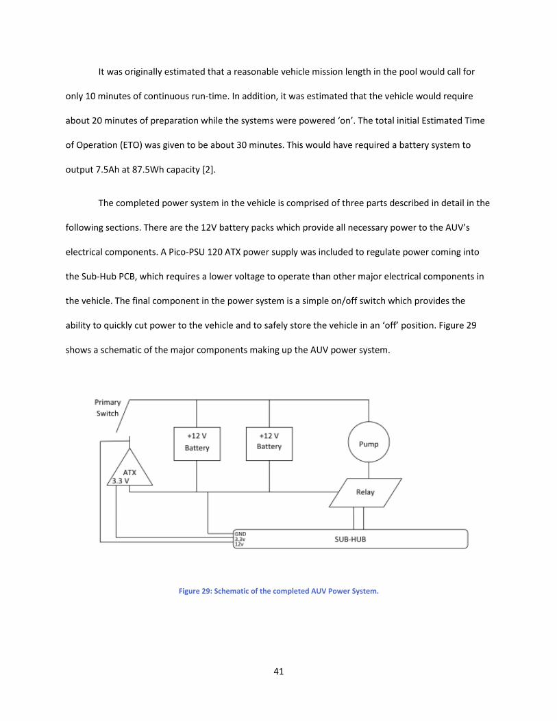
41

It was originally estimated that a reasonable vehicle mission length in the pool would call for

only 10 minutes of continuous run-time. In addition, it was estimated that the vehicle would require

about 20 minutes of preparation while the systems were powered ‘on’. The total initial Estimated Time

of Operation (ETO) was given to be about 30 minutes. This would have required a battery system to

output 7.5Ah at 87.5Wh capacity [2].

The completed power system in the vehicle is comprised of three parts described in detail in the

following sections. There are the 12V battery packs which provide all necessary power to the AUV’s

electrical components. A Pico-PSU 120 ATX power supply was included to regulate power coming into

the Sub-Hub PCB, which requires a lower voltage to operate than other major electrical components in

the vehicle. The final component in the power system is a simple on/off switch which provides the

ability to quickly cut power to the vehicle and to safely store the vehicle in an ‘off’ position. Figure 29

shows a schematic of the major components making up the AUV power system.

Figure 29: Schematic of the completed AUV Power System.

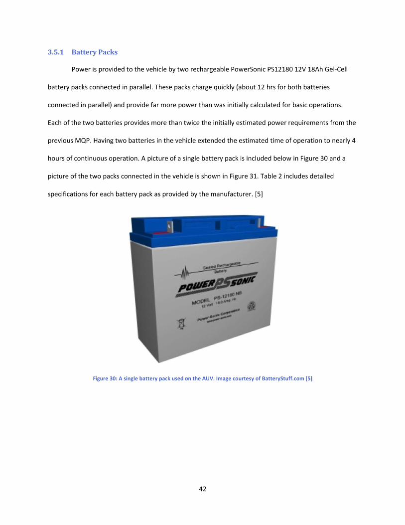
42

3.5.1 Battery Packs

Power is provided to the vehicle by two rechargeable PowerSonic PS12180 12V 18Ah Gel-Cell

battery packs connected in parallel. These packs charge quickly (about 12 hrs for both batteries

connected in parallel) and provide far more power than was initially calculated for basic operations.

Each of the two batteries provides more than twice the initially estimated power requirements from the

previous MQP. Having two batteries in the vehicle extended the estimated time of operation to nearly 4

hours of continuous operation. A picture of a single battery pack is included below in Figure 30 and a

picture of the two packs connected in the vehicle is shown in Figure 31. Table 2 includes detailed

specifications for each battery pack as provided by the manufacturer. [5]

Figure 30: A single battery pack used on the AUV. Image courtesy of BatteryStuff.com [5]

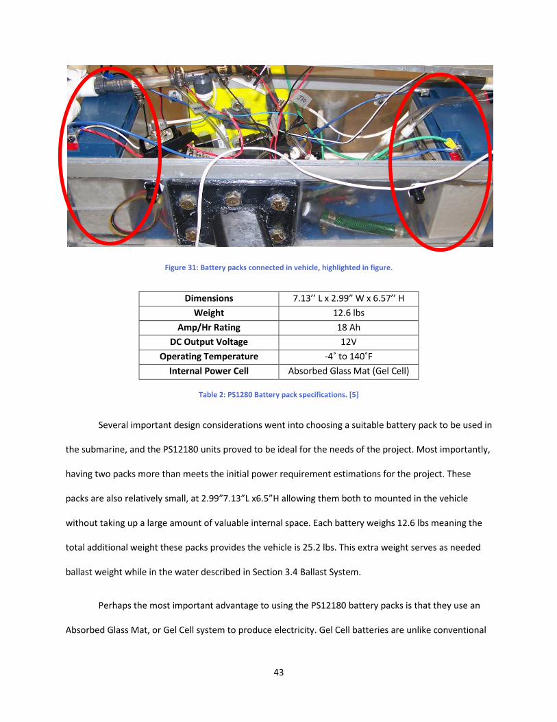
43

Figure 31: Battery packs connected in vehicle, highlighted in figure.

Dimensions 7.13’’ L x 2.99” W x 6.57’’ H

Weight 12.6 lbs

Amp/Hr Rating 18 Ah

DC Output Voltage 12V

Operating Temperature -4˚ to 140˚F

Internal Power Cell Absorbed Glass Mat (Gel Cell)

Table 2: PS1280 Battery pack specifications. [5]

Several important design considerations went into choosing a suitable battery pack to be used in

the submarine, and the PS12180 units proved to be ideal for the needs of the project. Most importantly,

having two packs more than meets the initial power requirement estimations for the project. These

packs are also relatively small, at 2.99”7.13”L x6.5”H allowing them both to mounted in the vehicle

without taking up a large amount of valuable internal space. Each battery weighs 12.6 lbs meaning the

total additional weight these packs provides the vehicle is 25.2 lbs. This extra weight serves as needed

ballast weight while in the water described in Section 3.4 Ballast System.

Perhaps the most important advantage to using the PS12180 battery packs is that they use an

Absorbed Glass Mat, or Gel Cell system to produce electricity. Gel Cell batteries are unlike conventional

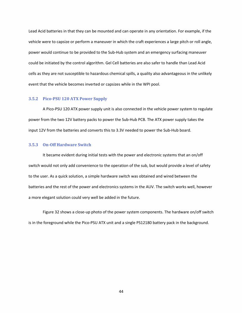
44

Lead Acid batteries in that they can be mounted and can operate in any orientation. For example, if the

vehicle were to capsize or perform a maneuver in which the craft experiences a large pitch or roll angle,

power would continue to be provided to the Sub-Hub system and an emergency surfacing maneuver

could be initiated by the control algorithm. Gel Cell batteries are also safer to handle than Lead Acid

cells as they are not susceptible to hazardous chemical spills, a quality also advantageous in the unlikely

event that the vehicle becomes inverted or capsizes while in the WPI pool.

3.5.2 Pico-PSU 120 ATX Power Supply

A Pico-PSU 120 ATX power supply unit is also connected in the vehicle power system to regulate

power from the two 12V battery packs to power the Sub-Hub PCB. The ATX power supply takes the

input 12V from the batteries and converts this to 3.3V needed to power the Sub-Hub board.

3.5.3 On-Off Hardware Switch

It became evident during initial tests with the power and electronic systems that an on/off

switch would not only add convenience to the operation of the sub, but would provide a level of safety

to the user. As a quick solution, a simple hardware switch was obtained and wired between the

batteries and the rest of the power and electronics systems in the AUV. The switch works well, however

a more elegant solution could very well be added in the future.

Figure 32 shows a close-up photo of the power system components. The hardware on/off switch

is in the foreground while the Pico-PSU ATX unit and a single PS12180 battery pack in the background.

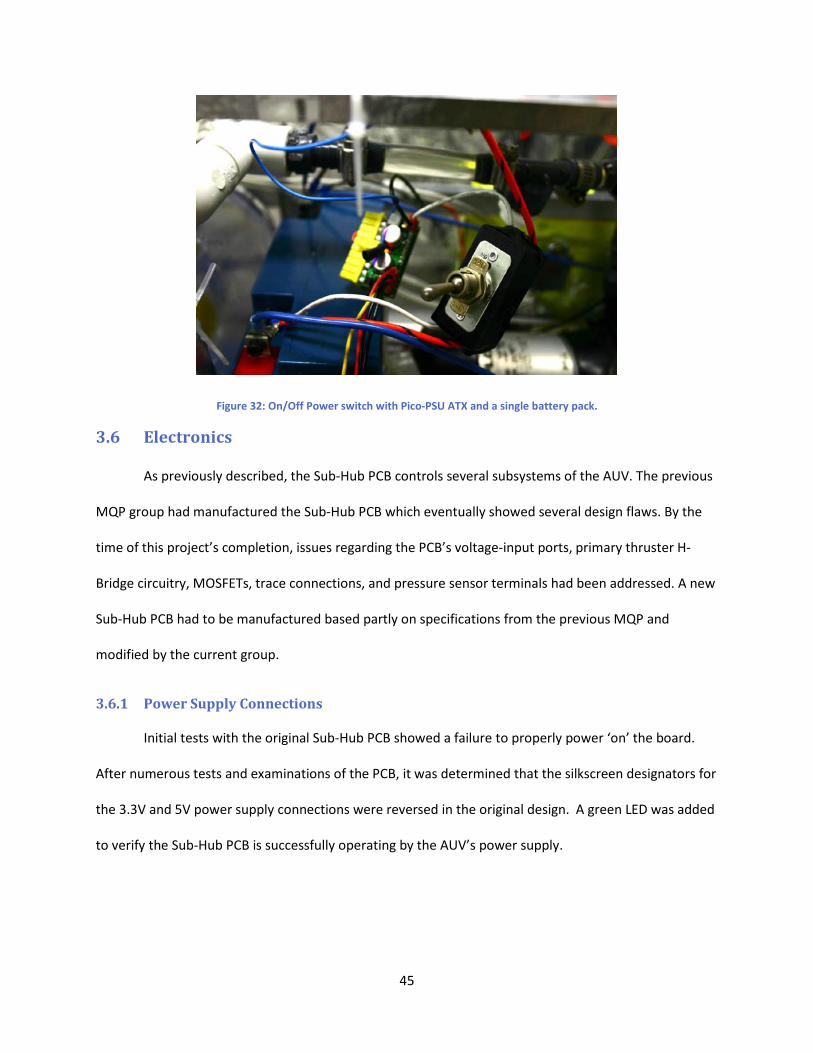
45

Figure 32: On/Off Power switch with Pico-PSU ATX and a single battery pack.

3.6 Electronics

As previously described, the Sub-Hub PCB controls several subsystems of the AUV. The previous

MQP group had manufactured the Sub-Hub PCB which eventually showed several design flaws. By the

time of this project’s completion, issues regarding the PCB’s voltage-input ports, primary thruster H-

Bridge circuitry, MOSFETs, trace connections, and pressure sensor terminals had been addressed. A new

Sub-Hub PCB had to be manufactured based partly on specifications from the previous MQP and

modified by the current group.

3.6.1 Power Supply Connections

Initial tests with the original Sub-Hub PCB showed a failure to properly power ‘on’ the board.

After numerous tests and examinations of the PCB, it was determined that the silkscreen designators for

the 3.3V and 5V power supply connections were reversed in the original design. A green LED was added

to verify the Sub-Hub PCB is successfully operating by the AUV’s power supply.

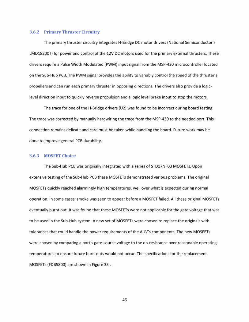
46

3.6.2 Primary Thruster Circuitry

The primary thruster circuitry integrates H-Bridge DC motor drivers (National Semiconductor’s

LMD18200T) for power and control of the 12V DC motors used for the primary external thrusters. These

drivers require a Pulse Width Modulated (PWM) input signal from the MSP-430 microcontroller located

on the Sub-Hub PCB. The PWM signal provides the ability to variably control the speed of the thruster’s

propellers and can run each primary thruster in opposing directions. The drivers also provide a logic-

level direction input to quickly reverse propulsion and a logic level brake input to stop the motors.

The trace for one of the H-Bridge drivers (U2) was found to be incorrect during board testing.

The trace was corrected by manually hardwiring the trace from the MSP-430 to the needed port. This

connection remains delicate and care must be taken while handling the board. Future work may be

done to improve general PCB durability.

3.6.3 MOSFET Choice

The Sub-Hub PCB was originally integrated with a series of STD17NF03 MOSFETs. Upon

extensive testing of the Sub-Hub PCB these MOSFETs demonstrated various problems. The original

MOSFETs quickly reached alarmingly high temperatures, well over what is expected during normal

operation. In some cases, smoke was seen to appear before a MOSFET failed. All these original MOSFETs

eventually burnt out. It was found that these MOSFETs were not applicable for the gate voltage that was

to be used in the Sub-Hub system. A new set of MOSFETs were chosen to replace the originals with

tolerances that could handle the power requirements of the AUV’s components. The new MOSFETs

were chosen by comparing a port’s gate-source voltage to the on-resistance over reasonable operating

temperatures to ensure future burn-outs would not occur. The specifications for the replacement

MOSFETs (FDB5800) are shown in Figure 33 .

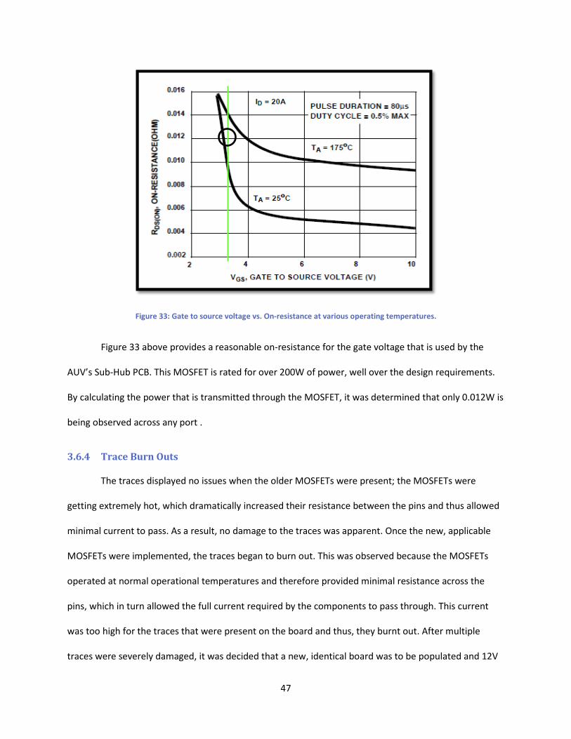
47

Figure 33: Gate to source voltage vs. On-resistance at various operating temperatures.

Figure 33 above provides a reasonable on-resistance for the gate voltage that is used by the

AUV’s Sub-Hub PCB. This MOSFET is rated for over 200W of power, well over the design requirements.

By calculating the power that is transmitted through the MOSFET, it was determined that only 0.012W is

being observed across any port .

3.6.4 Trace Burn Outs

The traces displayed no issues when the older MOSFETs were present; the MOSFETs were

getting extremely hot, which dramatically increased their resistance between the pins and thus allowed

minimal current to pass. As a result, no damage to the traces was apparent. Once the new, applicable

MOSFETs were implemented, the traces began to burn out. This was observed because the MOSFETs

operated at normal operational temperatures and therefore provided minimal resistance across the

pins, which in turn allowed the full current required by the components to pass through. This current

was too high for the traces that were present on the board and thus, they burnt out. After multiple

traces were severely damaged, it was decided that a new, identical board was to be populated and 12V

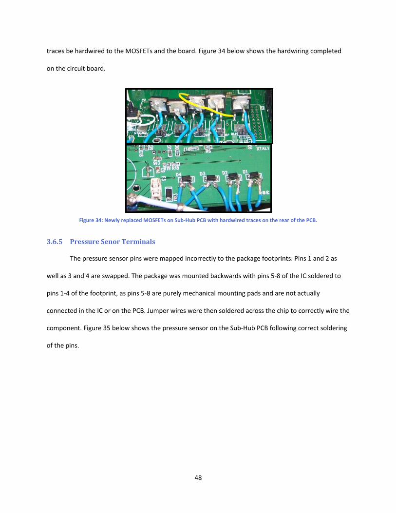
48

traces be hardwired to the MOSFETs and the board. Figure 34 below shows the hardwiring completed

on the circuit board.

Figure 34: Newly replaced MOSFETs on Sub-Hub PCB with hardwired traces on the rear of the PCB.

3.6.5 Pressure Senor Terminals

The pressure sensor pins were mapped incorrectly to the package footprints. Pins 1 and 2 as

well as 3 and 4 are swapped. The package was mounted backwards with pins 5-8 of the IC soldered to

pins 1-4 of the footprint, as pins 5-8 are purely mechanical mounting pads and are not actually

connected in the IC or on the PCB. Jumper wires were then soldered across the chip to correctly wire the

component. Figure 35 below shows the pressure sensor on the Sub-Hub PCB following correct soldering

of the pins.

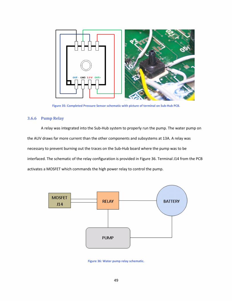
49

Figure 35: Completed Pressure Sensor schematic with picture of terminal on Sub-Hub PCB.

3.6.6 Pump Relay

A relay was integrated into the Sub-Hub system to properly run the pump. The water pump on

the AUV draws far more current than the other components and subsystems at 13A. A relay was

necessary to prevent burning out the traces on the Sub-Hub board where the pump was to be

interfaced. The schematic of the relay configuration is provided in Figure 36. Terminal J14 from the PCB

activates a MOSFET which commands the high power relay to control the pump.

Figure 36: Water pump relay schematic.

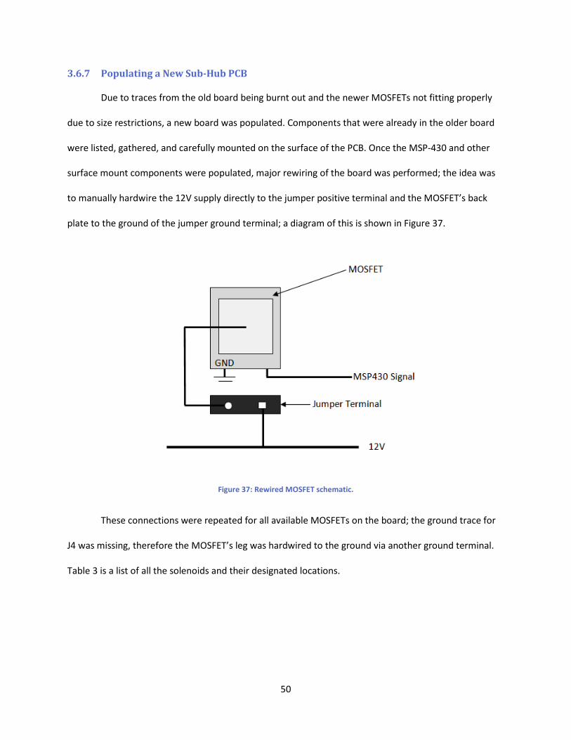
50

3.6.7 Populating a New Sub-Hub PCB

Due to traces from the old board being burnt out and the newer MOSFETs not fitting properly

due to size restrictions, a new board was populated. Components that were already in the older board

were listed, gathered, and carefully mounted on the surface of the PCB. Once the MSP-430 and other

surface mount components were populated, major rewiring of the board was performed; the idea was

to manually hardwire the 12V supply directly to the jumper positive terminal and the MOSFET’s back

plate to the ground of the jumper ground terminal; a diagram of this is shown in Figure 37.

Figure 37: Rewired MOSFET schematic.

These connections were repeated for all available MOSFETs on the board; the ground trace for

J4 was missing, therefore the MOSFET’s leg was hardwired to the ground via another ground terminal.

Table 3 is a list of all the solenoids and their designated locations.

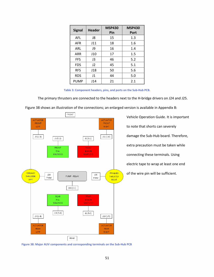
51

Signal Header MSP430

Pin MSP430

Port AFL J8 15 1.3 AFR J11 18 1.6 ARL J9 16 1.4 ARR J10 17 1.5 FFS J3 46 5.2 FDS J2 45 5.1 RFS J18 50 5.6 RDS J1 44 5.0

PUMP J14 21 2.1

Table 3: Component headers, pins, and ports on the Sub-Hub PCB.

The primary thrusters are connected to the headers next to the H-bridge drivers on J24 and J25.

Figure 38 shows an illustration of the connections; an enlarged version is available in Appendix B:

Vehicle Operation Guide. It is important

to note that shorts can severely

damage the Sub-Hub board. Therefore,

extra precaution must be taken while

connecting these terminals. Using

electric tape to wrap at least one end

of the wire pin will be sufficient.

Figure 38: Major AUV components and corresponding terminals on the Sub-Hub PCB

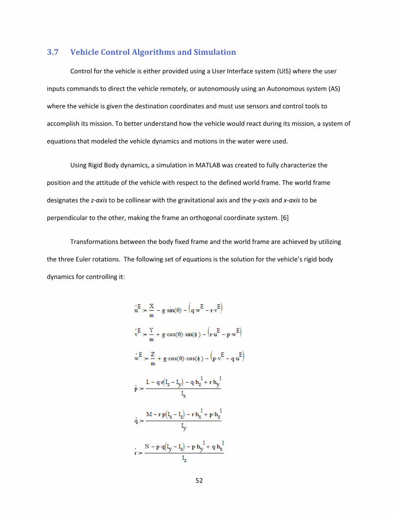
52

3.7 Vehicle Control Algorithms and Simulation

Control for the vehicle is either provided using a User Interface system (UIS) where the user

inputs commands to direct the vehicle remotely, or autonomously using an Autonomous system (AS)

where the vehicle is given the destination coordinates and must use sensors and control tools to

accomplish its mission. To better understand how the vehicle would react during its mission, a system of

equations that modeled the vehicle dynamics and motions in the water were used.

Using Rigid Body dynamics, a simulation in MATLAB was created to fully characterize the

position and the attitude of the vehicle with respect to the defined world frame. The world frame

designates the z-axis to be collinear with the gravitational axis and the y-axis and x-axis to be

perpendicular to the other, making the frame an orthogonal coordinate system. [6]

Transformations between the body fixed frame and the world frame are achieved by utilizing

the three Euler rotations. The following set of equations is the solution for the vehicle’s rigid body

dynamics for controlling it:

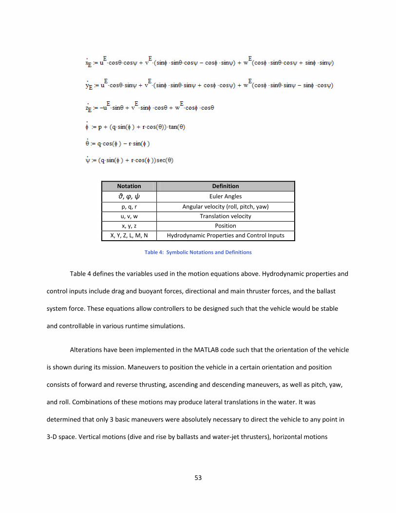
53

Notation Definition

θ, φ, ψ Euler Angles

p, q, r Angular velocity (roll, pitch, yaw)

u, v, w Translation velocity

x, y, z Position

X, Y, Z, L, M, N Hydrodynamic Properties and Control Inputs

Table 4: Symbolic Notations and Definitions

Table 4 defines the variables used in the motion equations above. Hydrodynamic properties and

control inputs include drag and buoyant forces, directional and main thruster forces, and the ballast

system force. These equations allow controllers to be designed such that the vehicle would be stable

and controllable in various runtime simulations.

Alterations have been implemented in the MATLAB code such that the orientation of the vehicle

is shown during its mission. Maneuvers to position the vehicle in a certain orientation and position

consists of forward and reverse thrusting, ascending and descending maneuvers, as well as pitch, yaw,

and roll. Combinations of these motions may produce lateral translations in the water. It was

determined that only 3 basic maneuvers were absolutely necessary to direct the vehicle to any point in

3-D space. Vertical motions (dive and rise by ballasts and water-jet thrusters), horizontal motions

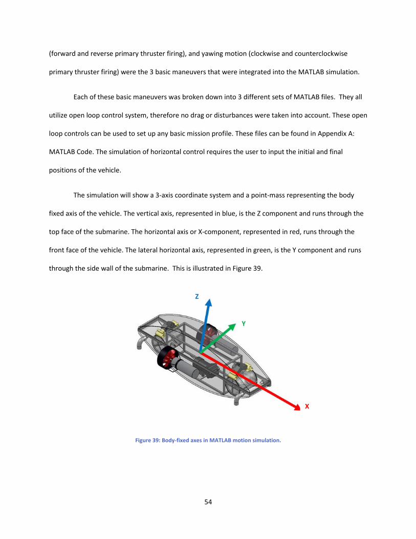
54

(forward and reverse primary thruster firing), and yawing motion (clockwise and counterclockwise

primary thruster firing) were the 3 basic maneuvers that were integrated into the MATLAB simulation.

Each of these basic maneuvers was broken down into 3 different sets of MATLAB files. They all

utilize open loop control system, therefore no drag or disturbances were taken into account. These open

loop controls can be used to set up any basic mission profile. These files can be found in Appendix A:

MATLAB Code. The simulation of horizontal control requires the user to input the initial and final

positions of the vehicle.

The simulation will show a 3-axis coordinate system and a point-mass representing the body

fixed axis of the vehicle. The vertical axis, represented in blue, is the Z component and runs through the

top face of the submarine. The horizontal axis or X-component, represented in red, runs through the

front face of the vehicle. The lateral horizontal axis, represented in green, is the Y component and runs

through the side wall of the submarine. This is illustrated in Figure 39.

Figure 39: Body-fixed axes in MATLAB motion simulation.

X

Y

Z

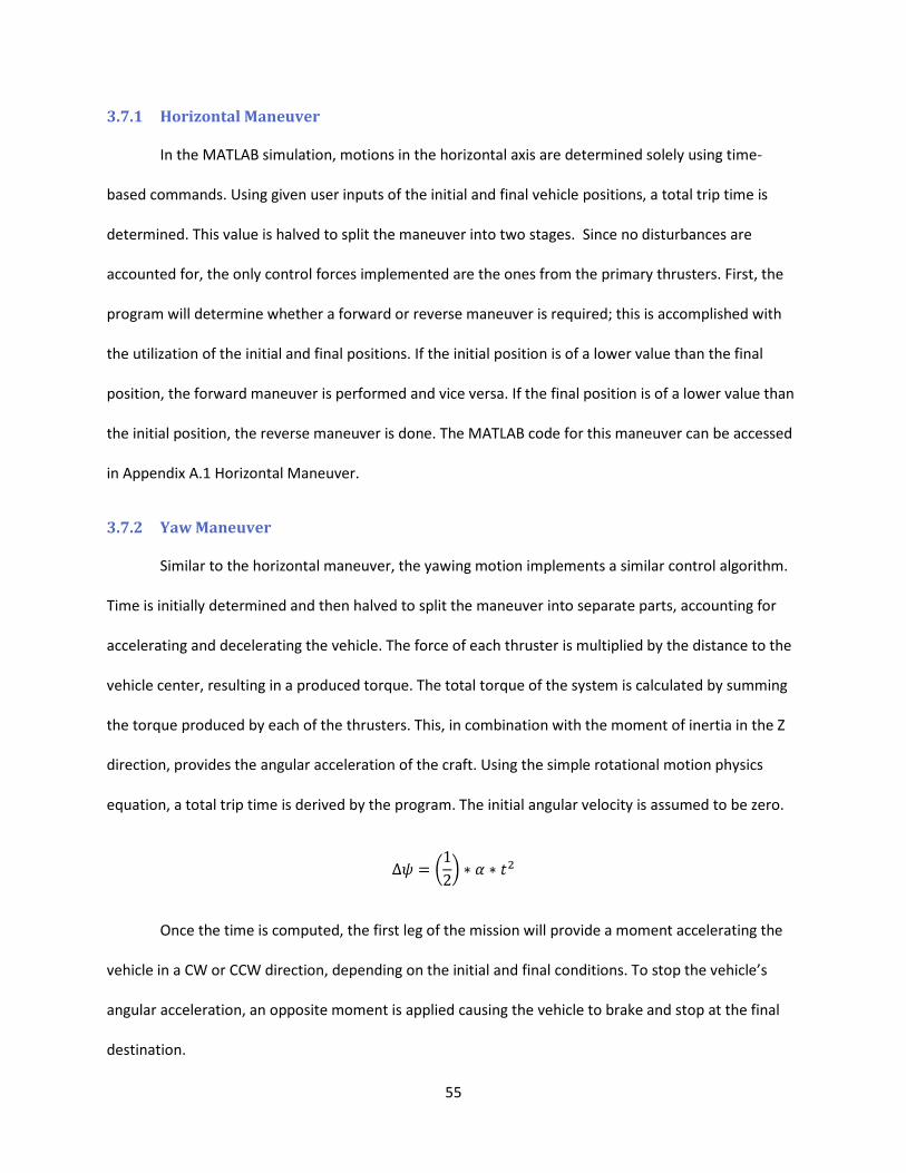
55

3.7.1 Horizontal Maneuver

In the MATLAB simulation, motions in the horizontal axis are determined solely using time-

based commands. Using given user inputs of the initial and final vehicle positions, a total trip time is

determined. This value is halved to split the maneuver into two stages. Since no disturbances are

accounted for, the only control forces implemented are the ones from the primary thrusters. First, the

program will determine whether a forward or reverse maneuver is required; this is accomplished with

the utilization of the initial and final positions. If the initial position is of a lower value than the final

position, the forward maneuver is performed and vice versa. If the final position is of a lower value than

the initial position, the reverse maneuver is done. The MATLAB code for this maneuver can be accessed

in Appendix A.1 Horizontal Maneuver.

3.7.2 Yaw Maneuver

Similar to the horizontal maneuver, the yawing motion implements a similar control algorithm.

Time is initially determined and then halved to split the maneuver into separate parts, accounting for

accelerating and decelerating the vehicle. The force of each thruster is multiplied by the distance to the

vehicle center, resulting in a produced torque. The total torque of the system is calculated by summing

the torque produced by each of the thrusters. This, in combination with the moment of inertia in the Z

direction, provides the angular acceleration of the craft. Using the simple rotational motion physics

equation, a total trip time is derived by the program. The initial angular velocity is assumed to be zero.

Once the time is computed, the first leg of the mission will provide a moment accelerating the

vehicle in a CW or CCW direction, depending on the initial and final conditions. To stop the vehicle’s

angular acceleration, an opposite moment is applied causing the vehicle to brake and stop at the final

destination.

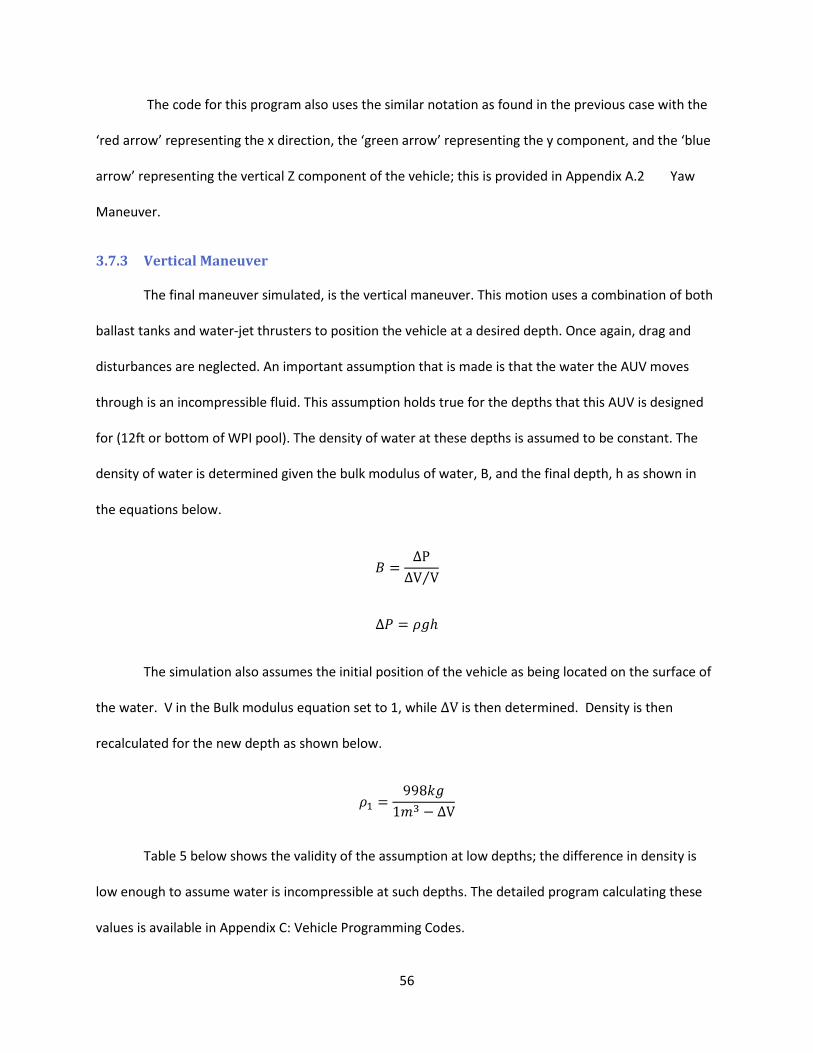
56

The code for this program also uses the similar notation as found in the previous case with the

‘red arrow’ representing the x direction, the ‘green arrow’ representing the y component, and the ‘blue

arrow’ representing the vertical Z component of the vehicle; this is provided in Appendix A.2 Yaw

Maneuver.

3.7.3 Vertical Maneuver

The final maneuver simulated, is the vertical maneuver. This motion uses a combination of both

ballast tanks and water-jet thrusters to position the vehicle at a desired depth. Once again, drag and

disturbances are neglected. An important assumption that is made is that the water the AUV moves

through is an incompressible fluid. This assumption holds true for the depths that this AUV is designed

for (12ft or bottom of WPI pool). The density of water at these depths is assumed to be constant. The

density of water is determined given the bulk modulus of water, B, and the final depth, h as shown in

the equations below.

The simulation also assumes the initial position of the vehicle as being located on the surface of

the water. V in the Bulk modulus equation set to 1, while is then determined. Density is then

recalculated for the new depth as shown below.

Table 5 below shows the validity of the assumption at low depths; the difference in density is

low enough to assume water is incompressible at such depths. The detailed program calculating these

values is available in Appendix C: Vehicle Programming Codes.

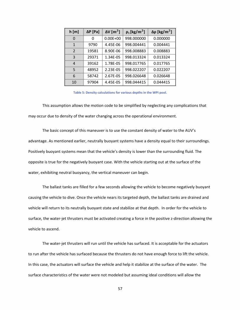
57

h [m] ΔP [Pa] ΔV [ ] ρ1 [kg/ ] Δρ [kg/ ]

0 0 0.00E+00 998.000000 0.000000

1 9790 4.45E-06 998.004441 0.004441

2 19581 8.90E-06 998.008883 0.008883

3 29371 1.34E-05 998.013324 0.013324

4 39162 1.78E-05 998.017765 0.017765

5 48952 2.23E-05 998.022207 0.022207

6 58742 2.67E-05 998.026648 0.026648

10 97904 4.45E-05 998.044415 0.044415

Table 5: Density calculations for various depths in the WPI pool.

This assumption allows the motion code to be simplified by neglecting any complications that

may occur due to density of the water changing across the operational environment.

The basic concept of this maneuver is to use the constant density of water to the AUV’s

advantage. As mentioned earlier, neutrally buoyant systems have a density equal to their surroundings.

Positively buoyant systems mean that the vehicle’s density is lower than the surrounding fluid. The

opposite is true for the negatively buoyant case. With the vehicle starting out at the surface of the

water, exhibiting neutral buoyancy, the vertical maneuver can begin.

The ballast tanks are filled for a few seconds allowing the vehicle to become negatively buoyant

causing the vehicle to dive. Once the vehicle nears its targeted depth, the ballast tanks are drained and

vehicle will return to its neutrally buoyant state and stabilize at that depth. In order for the vehicle to

surface, the water-jet thrusters must be activated creating a force in the positive z-direction allowing the

vehicle to ascend.

The water-jet thrusters will run until the vehicle has surfaced. It is acceptable for the actuators

to run after the vehicle has surfaced because the thrusters do not have enough force to lift the vehicle.

In this case, the actuators will surface the vehicle and help it stabilize at the surface of the water. The

surface characteristics of the water were not modeled but assuming ideal conditions will allow the

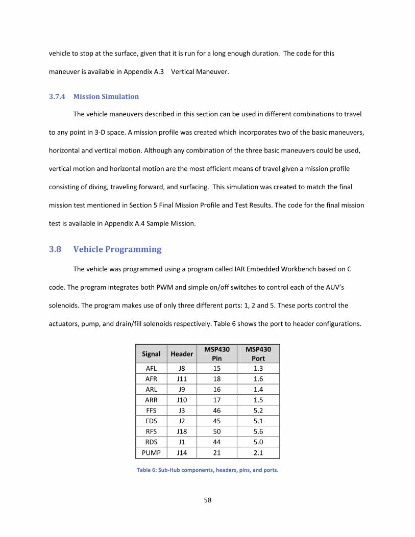
58

vehicle to stop at the surface, given that it is run for a long enough duration. The code for this

maneuver is available in Appendix A.3 Vertical Maneuver.

3.7.4 Mission Simulation

The vehicle maneuvers described in this section can be used in different combinations to travel

to any point in 3-D space. A mission profile was created which incorporates two of the basic maneuvers,

horizontal and vertical motion. Although any combination of the three basic maneuvers could be used,

vertical motion and horizontal motion are the most efficient means of travel given a mission profile

consisting of diving, traveling forward, and surfacing. This simulation was created to match the final

mission test mentioned in Section 5 Final Mission Profile and Test Results. The code for the final mission

test is available in Appendix A.4 Sample Mission.

3.8 Vehicle Programming

The vehicle was programmed using a program called IAR Embedded Workbench based on C

code. The program integrates both PWM and simple on/off switches to control each of the AUV’s

solenoids. The program makes use of only three different ports: 1, 2 and 5. These ports control the

actuators, pump, and drain/fill solenoids respectively. Table 6 shows the port to header configurations.

Signal Header MSP430

Pin MSP430

Port AFL J8 15 1.3 AFR J11 18 1.6 ARL J9 16 1.4 ARR J10 17 1.5 FFS J3 46 5.2 FDS J2 45 5.1 RFS J18 50 5.6 RDS J1 44 5.0

PUMP J14 21 2.1

Table 6: Sub-Hub components, headers, pins, and ports.

59

Switch Delays have been implemented into the code for running a certain task for a given time.

It has not been fully configured with real time; although, a simple calibration process will allow it to run

more precisely. It is imperative that at least one of the solenoids be open before running the pump. In

addition, the solenoids should be turned off only after the pump is powered off to avoid over

pressurizing the fluid lines. Having a short switch delay in between operation will suffice.

Numerous problems have occurred with this software. On several occasions the computer

would freeze and a manual termination was required. These problems can signify a problem with the

sub-hub board such as a short circuit. The overall process is simple; once the connections found in Table

6 are connected and the JTAG Debugger unit is connected to the sub-hub board, activate the IAR

Workbench on a computer and open a workspace. Make sure that the compiler is set to ‘Debugger’

mode and the MSP430F233 unit is selected. Step through the programs lines of code once to make sure

the components are functional. The PWM code requires the code be fully run. Stepping through the

code will not work.

In the PWM code, the velocity of the thrusters can be controlled by varying the DESTRX values

from 0 to 5220. A value of 5220 would provide maximum thrust. These codes and others are available in

Appendix C: Vehicle Programming Codes.

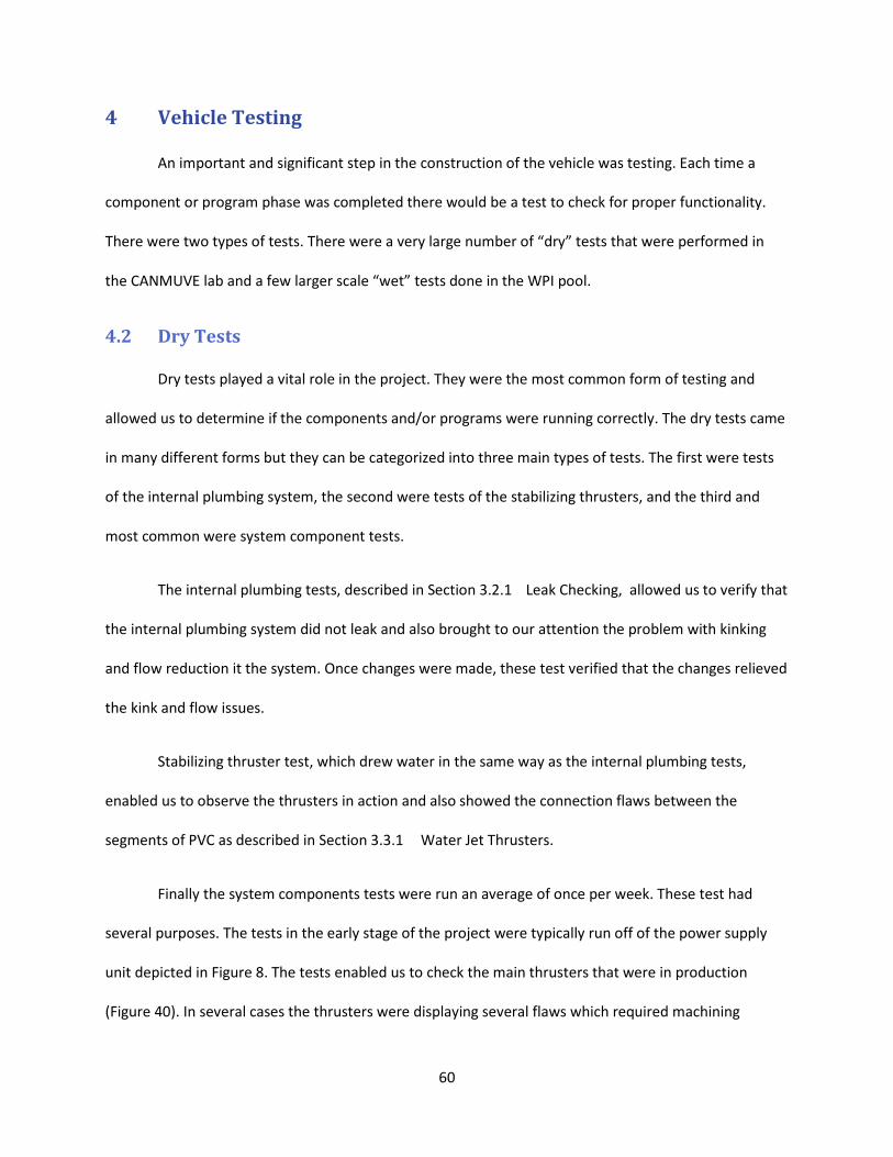
60

4 Vehicle Testing

An important and significant step in the construction of the vehicle was testing. Each time a

component or program phase was completed there would be a test to check for proper functionality.

There were two types of tests. There were a very large number of “dry” tests that were performed in

the CANMUVE lab and a few larger scale “wet” tests done in the WPI pool.

4.2 Dry Tests

Dry tests played a vital role in the project. They were the most common form of testing and

allowed us to determine if the components and/or programs were running correctly. The dry tests came

in many different forms but they can be categorized into three main types of tests. The first were tests

of the internal plumbing system, the second were tests of the stabilizing thrusters, and the third and

most common were system component tests.

The internal plumbing tests, described in Section 3.2.1 Leak Checking, allowed us to verify that

the internal plumbing system did not leak and also brought to our attention the problem with kinking

and flow reduction it the system. Once changes were made, these test verified that the changes relieved

the kink and flow issues.

Stabilizing thruster test, which drew water in the same way as the internal plumbing tests,

enabled us to observe the thrusters in action and also showed the connection flaws between the

segments of PVC as described in Section 3.3.1 Water Jet Thrusters.

Finally the system components tests were run an average of once per week. These test had

several purposes. The tests in the early stage of the project were typically run off of the power supply

unit depicted in Figure 8. The tests enabled us to check the main thrusters that were in production

(Figure 40). In several cases the thrusters were displaying several flaws which required machining

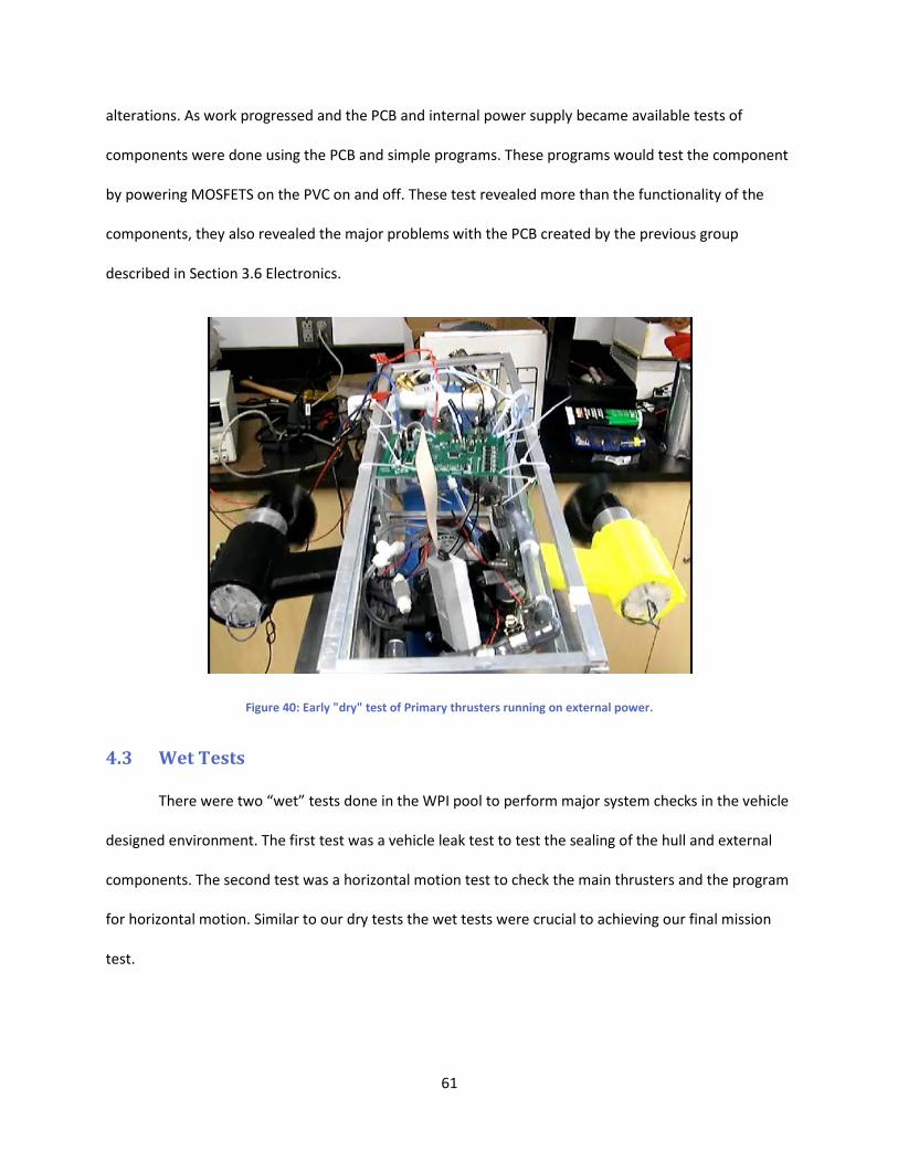
61

alterations. As work progressed and the PCB and internal power supply became available tests of

components were done using the PCB and simple programs. These programs would test the component

by powering MOSFETS on the PVC on and off. These test revealed more than the functionality of the

components, they also revealed the major problems with the PCB created by the previous group

described in Section 3.6 Electronics.

Figure 40: Early "dry" test of Primary thrusters running on external power.

4.3 Wet Tests

There were two “wet” tests done in the WPI pool to perform major system checks in the vehicle

designed environment. The first test was a vehicle leak test to test the sealing of the hull and external

components. The second test was a horizontal motion test to check the main thrusters and the program

for horizontal motion. Similar to our dry tests the wet tests were crucial to achieving our final mission

test.

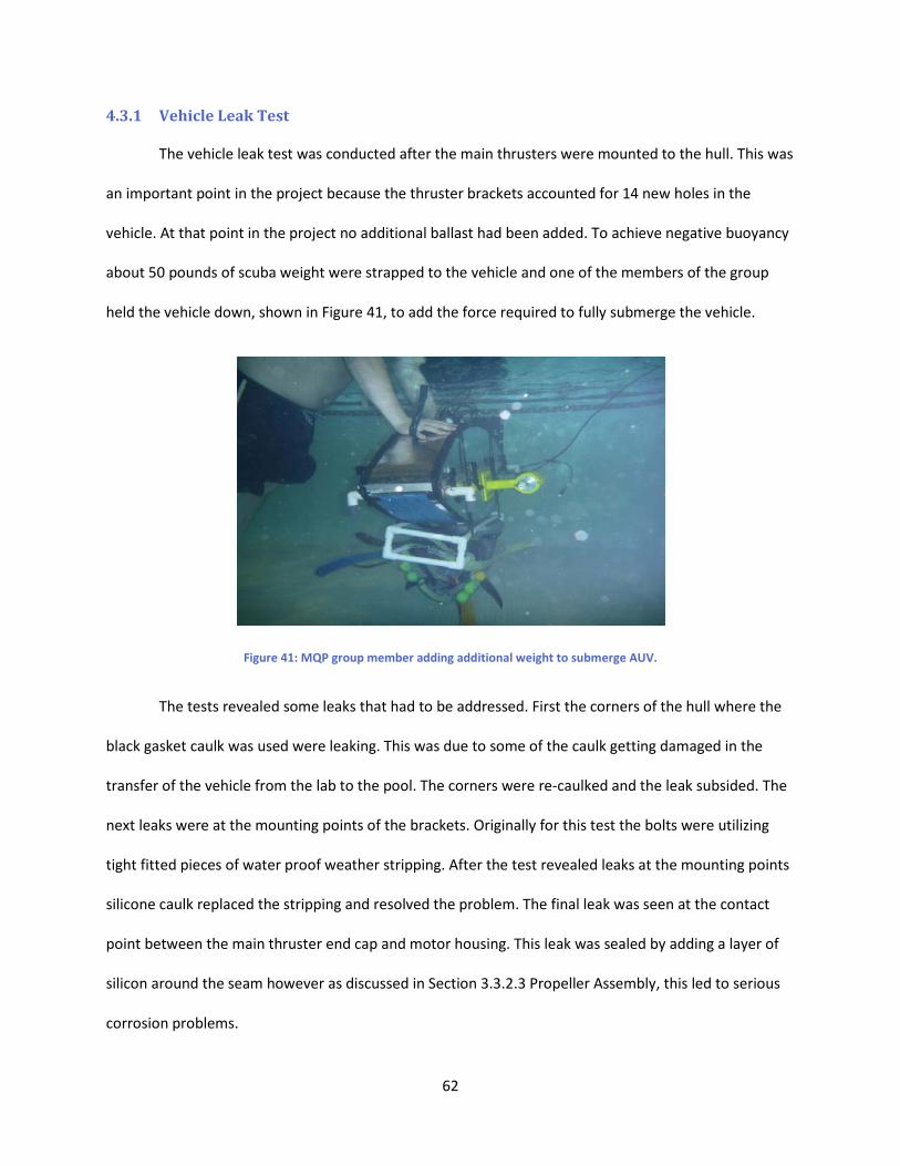
62

4.3.1 Vehicle Leak Test

The vehicle leak test was conducted after the main thrusters were mounted to the hull. This was

an important point in the project because the thruster brackets accounted for 14 new holes in the

vehicle. At that point in the project no additional ballast had been added. To achieve negative buoyancy

about 50 pounds of scuba weight were strapped to the vehicle and one of the members of the group

held the vehicle down, shown in Figure 41, to add the force required to fully submerge the vehicle.

Figure 41: MQP group member adding additional weight to submerge AUV.

The tests revealed some leaks that had to be addressed. First the corners of the hull where the

black gasket caulk was used were leaking. This was due to some of the caulk getting damaged in the

transfer of the vehicle from the lab to the pool. The corners were re-caulked and the leak subsided. The

next leaks were at the mounting points of the brackets. Originally for this test the bolts were utilizing

tight fitted pieces of water proof weather stripping. After the test revealed leaks at the mounting points

silicone caulk replaced the stripping and resolved the problem. The final leak was seen at the contact

point between the main thruster end cap and motor housing. This leak was sealed by adding a layer of

silicon around the seam however as discussed in Section 3.3.2.3 Propeller Assembly, this led to serious

corrosion problems.

63

4.3.2 Horizontal Motion Test

The goal of the horizontal motion test was to observe the vehicle perform horizontal motion to

a prescribed distance. Prior to running the test a leak test was performed to ensure the additional

sealing measures taken after the first leak test were sufficient. All areas with prior leaking had no

noticeable leaks. Next a test of the program was run on the vehicle out of the water. The program

powered the main thrusters on at full power (Figure 42) for a set amount of time determined on site and

added into the program. The thrusters powered on and the program ran successfully. Next the same

test was run in the water. The thrusters powered on but an unexpected and drastic decline in

performance was observed. The water is a much high density medium air and was causing the propellers

to slowly slide off of the thruster. With each bit of increase in slipping the performance of the thrusters

was reduced. It was this test that caused us to design the cowl described in Section 3.3.2.4 Propeller

Cowl, and two new propellers with slightly smaller inner diameters to hold onto the end caps more

tightly. The test was conducted several times with the same slipping however by the end of testing the

performance of the thrusters was degrading even more. When the vehicle was back in the lab a multi-

meter showed the motors were giving a resistance of several thousand ohms when they should give

about 3-6 ohms of resistance. A resistance that high triggered the possibility of corrosion and after

removing the motors it was verified that corrosion caused the failure.

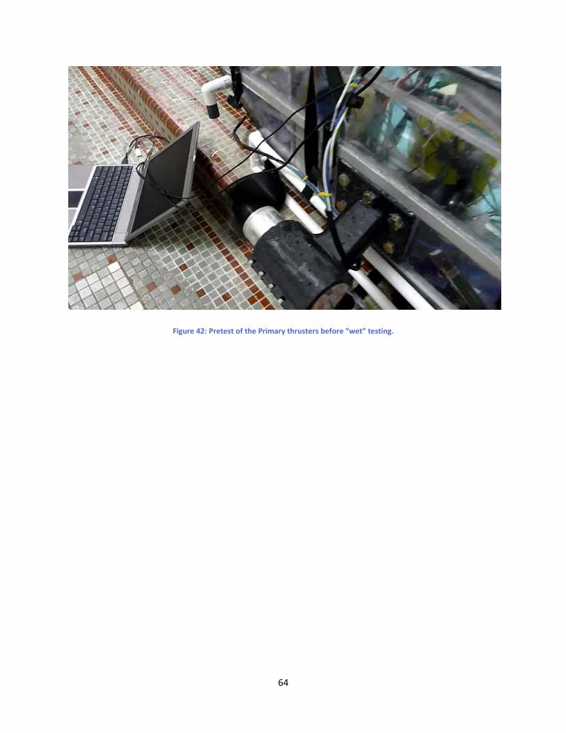
64

Figure 42: Pretest of the Primary thrusters before “wet” testing.

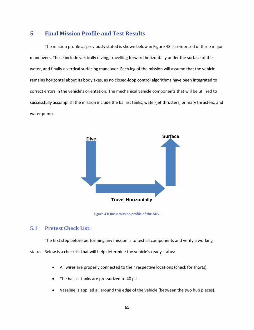
65

5 Final Mission Profile and Test Results

The mission profile as previously stated is shown below in Figure 43 is comprised of three major

maneuvers. These include vertically diving, travelling forward horizontally under the surface of the

water, and finally a vertical surfacing maneuver. Each leg of the mission will assume that the vehicle

remains horizontal about its body axes, as no closed-loop control algorithms have been integrated to

correct errors in the vehicle’s orientation. The mechanical vehicle components that will be utilized to

successfully accomplish the mission include the ballast tanks, water-jet thrusters, primary thrusters, and

water pump.

Figure 43: Basic mission profile of the AUV.

5.1 Pretest Check List:

The first step before performing any mission is to test all components and verify a working

status. Below is a checklist that will help determine the vehicle’s ready status:

• All wires are properly connected to their respective locations (check for shorts).

• The ballast tanks are pressurized to 40 psi.

• Vaseline is applied all around the edge of the vehicle (between the two hub pieces).

Dive

Travel Horizontally

Surface

66

• Vaseline is reapplied on the outside edges of the vehicle.

• Run the file named ‘SystemCheck’ by stepping through the program – health of the

system can be determined both visually and audibly.

o A ‘strong click’ will be heard when the solenoids have been turned ‘on’.

o A ‘low dub’ will be heard when the solenoids have been turned ‘off’.

o The pump can be heard operating.

• Run the file named ‘PWM’ and check primary thruster operation.

5.1.1 Achieving Neutral Buoyancy

Ensure all ballast weights are properly distributed so that the vehicle will demonstrate static

stability on the surface of the water. It is important to note that neutral buoyancy is to be achieved only

after the pipelines are filled with water and any air bubbles displaced. Therefore, the lines in the liquid

system must be purged of all air before determining if the ballast weight is correct.

5.1.2 System Air Purge

The goal of a system purge is to eliminate any air gaps or bubbles present in the pipelines. This

can be accomplished by first turning on all solenoids and then running the pump for a few seconds. The

pump must then be shut off before the solenoids.

5.2 Description of Mission Stages and Maneuvers

Included in the sections below are more detailed analyses and descriptions of each maneuver

performed by the AUV during the three maneuvers of the basic mission profile. Each maneuver is split

into a ‘stage’ and described sequentially as experienced by the AUV while in the water. Refer to

Appendix B: Vehicle Operation Guide for a diagram of component and wire positions.

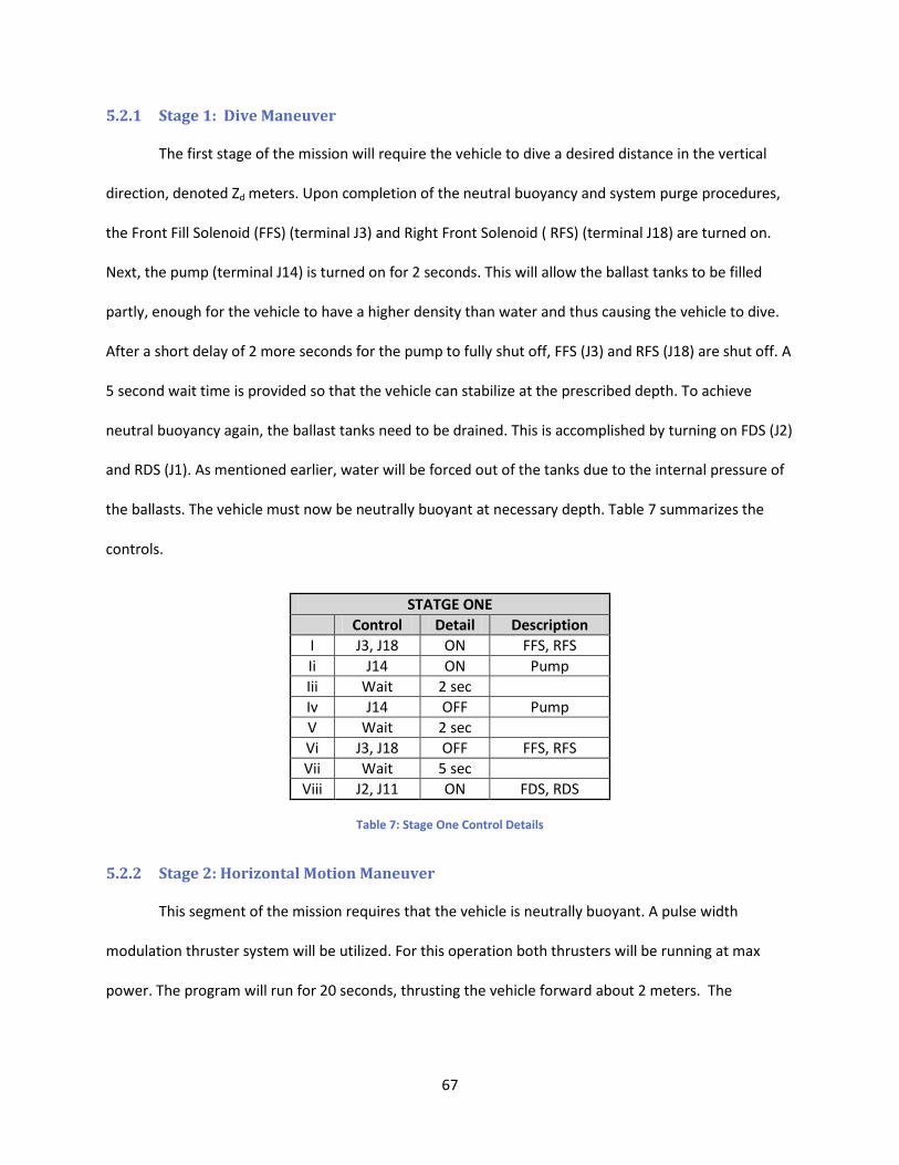
67

5.2.1 Stage 1: Dive Maneuver

The first stage of the mission will require the vehicle to dive a desired distance in the vertical

direction, denoted Zd meters. Upon completion of the neutral buoyancy and system purge procedures,

the Front Fill Solenoid (FFS) (terminal J3) and Right Front Solenoid ( RFS) (terminal J18) are turned on.

Next, the pump (terminal J14) is turned on for 2 seconds. This will allow the ballast tanks to be filled

partly, enough for the vehicle to have a higher density than water and thus causing the vehicle to dive.

After a short delay of 2 more seconds for the pump to fully shut off, FFS (J3) and RFS (J18) are shut off. A

5 second wait time is provided so that the vehicle can stabilize at the prescribed depth. To achieve

neutral buoyancy again, the ballast tanks need to be drained. This is accomplished by turning on FDS (J2)

and RDS (J1). As mentioned earlier, water will be forced out of the tanks due to the internal pressure of

the ballasts. The vehicle must now be neutrally buoyant at necessary depth. Table 7 summarizes the

controls.

STATGE ONE

Control Detail Description

I J3, J18 ON FFS, RFS Ii J14 ON Pump Iii Wait 2 sec

Iv J14 OFF Pump V Wait 2 sec

Vi J3, J18 OFF FFS, RFS Vii Wait 5 sec

Viii J2, J11 ON FDS, RDS

Table 7: Stage One Control Details

5.2.2 Stage 2: Horizontal Motion Maneuver

This segment of the mission requires that the vehicle is neutrally buoyant. A pulse width

modulation thruster system will be utilized. For this operation both thrusters will be running at max

power. The program will run for 20 seconds, thrusting the vehicle forward about 2 meters. The

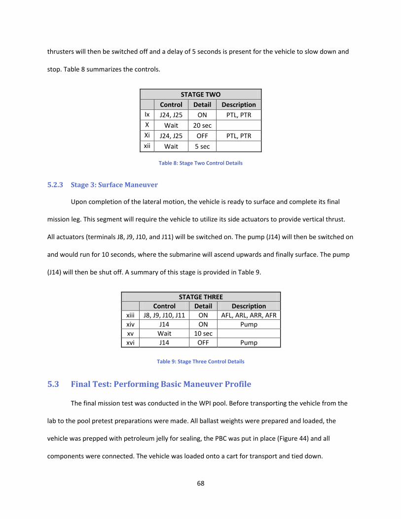
68

thrusters will then be switched off and a delay of 5 seconds is present for the vehicle to slow down and

stop. Table 8 summarizes the controls.

STATGE TWO

Control Detail Description

Ix J24, J25 ON PTL, PTR X Wait 20 sec

Xi J24, J25 OFF PTL, PTR xii Wait 5 sec

Table 8: Stage Two Control Details

5.2.3 Stage 3: Surface Maneuver

Upon completion of the lateral motion, the vehicle is ready to surface and complete its final

mission leg. This segment will require the vehicle to utilize its side actuators to provide vertical thrust.

All actuators (terminals J8, J9, J10, and J11) will be switched on. The pump (J14) will then be switched on

and would run for 10 seconds, where the submarine will ascend upwards and finally surface. The pump

(J14) will then be shut off. A summary of this stage is provided in Table 9.

Table 9: Stage Three Control Details

5.3 Final Test: Performing Basic Maneuver Profile

The final mission test was conducted in the WPI pool. Before transporting the vehicle from the

lab to the pool pretest preparations were made. All ballast weights were prepared and loaded, the

vehicle was prepped with petroleum jelly for sealing, the PBC was put in place (Figure 44) and all

components were connected. The vehicle was loaded onto a cart for transport and tied down.

STATGE THREE

Control Detail Description

xiii J8, J9, J10, J11 ON AFL, ARL, ARR, AFR xiv J14 ON Pump xv Wait 10 sec

xvi J14 OFF Pump

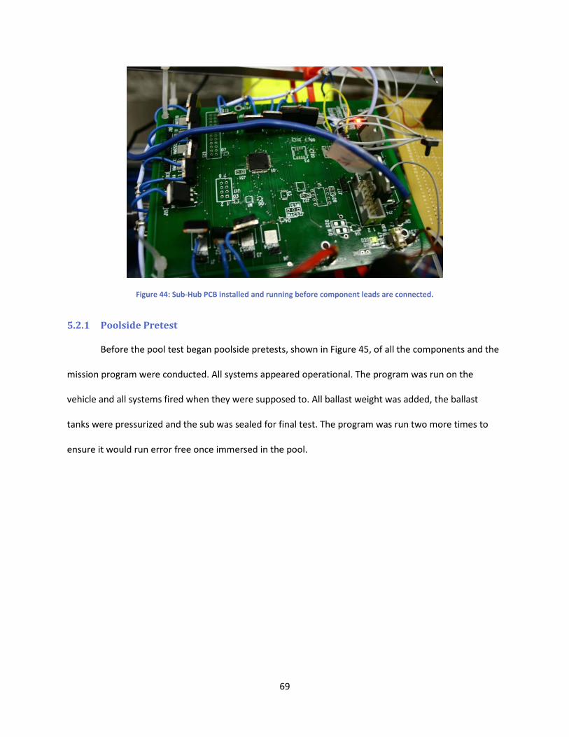
69

Figure 44: Sub-Hub PCB installed and running before component leads are connected.

5.2.1 Poolside Pretest

Before the pool test began poolside pretests, shown in Figure 45, of all the components and the

mission program were conducted. All systems appeared operational. The program was run on the

vehicle and all systems fired when they were supposed to. All ballast weight was added, the ballast

tanks were pressurized and the sub was sealed for final test. The program was run two more times to

ensure it would run error free once immersed in the pool.

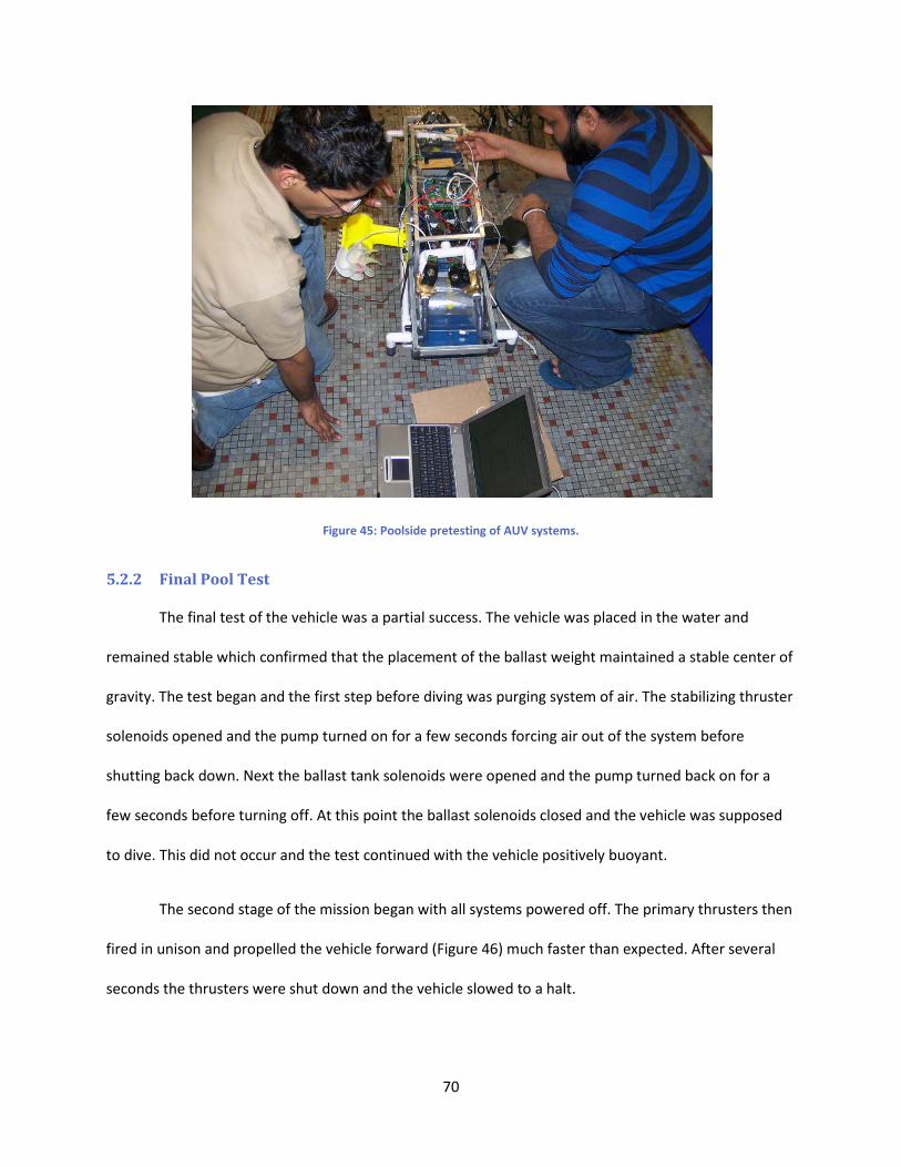
70

Figure 45: Poolside pretesting of AUV systems.

5.2.2 Final Pool Test

The final test of the vehicle was a partial success. The vehicle was placed in the water and

remained stable which confirmed that the placement of the ballast weight maintained a stable center of

gravity. The test began and the first step before diving was purging system of air. The stabilizing thruster

solenoids opened and the pump turned on for a few seconds forcing air out of the system before

shutting back down. Next the ballast tank solenoids were opened and the pump turned back on for a

few seconds before turning off. At this point the ballast solenoids closed and the vehicle was supposed

to dive. This did not occur and the test continued with the vehicle positively buoyant.

The second stage of the mission began with all systems powered off. The primary thrusters then

fired in unison and propelled the vehicle forward (Figure 46) much faster than expected. After several

seconds the thrusters were shut down and the vehicle slowed to a halt.

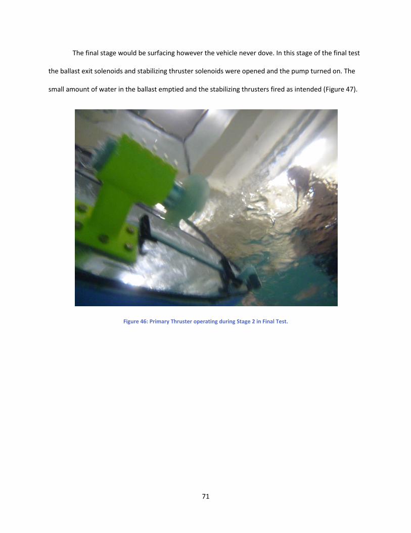
71

The final stage would be surfacing however the vehicle never dove. In this stage of the final test

the ballast exit solenoids and stabilizing thruster solenoids were opened and the pump turned on. The

small amount of water in the ballast emptied and the stabilizing thrusters fired as intended (Figure 47).

Figure 46: Primary Thruster operating during Stage 2 in Final Test.

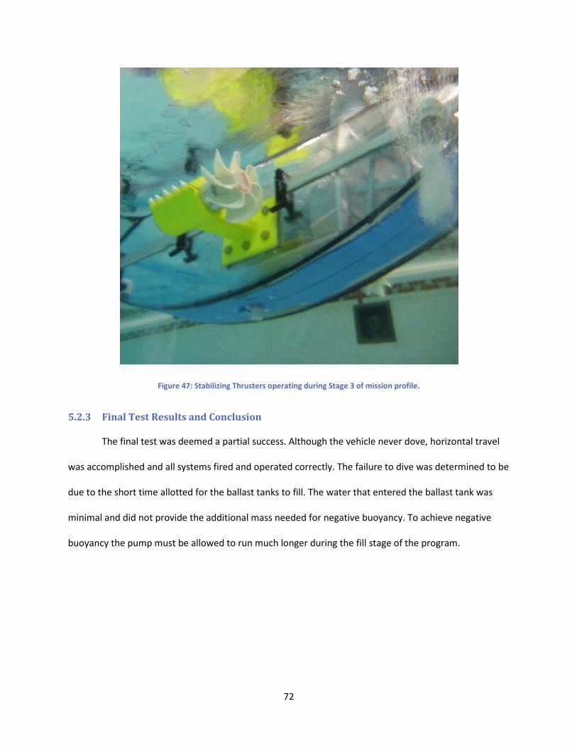
72

Figure 47: Stabilizing Thrusters operating during Stage 3 of mission profile.

5.2.3 Final Test Results and Conclusion

The final test was deemed a partial success. Although the vehicle never dove, horizontal travel

was accomplished and all systems fired and operated correctly. The failure to dive was determined to be

due to the short time allotted for the ballast tanks to fill. The water that entered the ballast tank was

minimal and did not provide the additional mass needed for negative buoyancy. To achieve negative

buoyancy the pump must be allowed to run much longer during the fill stage of the program.

73

6 Future Work and Recommendations

After almost eight months of work several significant strides were made towards complete

autonomous motion. However, several things need to be done and optimized before complete

autonomy is accomplished.

Our first recommendation for a group beginning work on the vehicle is to refer to a Vehicle

Operation Guide found in Appendix B: Vehicle Operation Guide. This guide will help expedite the initial

learning process and enable proper set up and handling of the vehicle and components without time

killing errors.

Next, there are a few recommendations for the primary thrusters to help optimize performance

and ease the assembly and disassembly processes. The motor housing and end caps should be

redesigned and machined to utilize a screw-on system similar to the end of a flashlight or thermos. This

will make it easy to assemble and disassemble the thruster and ensure a tight and secure fitting. Also

the new replacement motors are much shorter than the old motors, a smaller motor housing could be

utilized and help reduce the size of the thrusters. Machining of the parts should be done by CNC to save

time, ensure high tolerance, and allow focus to be placed on other essential objectives. Also the cowl

described in Section 3.3.2.4 Propeller Cowl, should be manufactured and installed on the thruster

assembly to prevent propeller slippage and provide protection against fracturing the brittle propeller

blades.

The current main thruster assembly still produces unacceptable drag due to the flat face of the

front end cap. It is recommended that the nose cone described in Section 3.3.2.5 Nose Cone, be

machined and installed to make the assembly more hydrodynamic.

74

The next recommendation deals with more efficient ballast weight placement. As of the end of

our work on the vehicle two 25 pound sacks of lead weight are set in the sub in front of the motor and

laid on top of the motor. These sacks are taking up valuable space that will be needed when

implementing other sensors including the three axis sonar system developed by WPI graduate student

Russel Morrin.

One major concern with the vehicle was the possibility of a single point catastrophic failure in

the vehicle. The PCB, pump relay, and any other electronics that get installed in the vehicle are located

directly above the internal plumbing system. If the tubing should leak or rupture it could short the

electronics and cause a catastrophic failure in the vehicle. To avoid this there is a temporary sheet of

Lexan placed above the plumbing system to help deter any water if a leak occurs. It is recommended

that a permanent, easily removable barrier be installed between the tubing and the electronics to

safeguard them from leakage.

In addition, the internal framework of the vehicle is all aluminum. This is highly conductive and if

a battery or other electronic component shift and come in contact with the frame it can cause shorts

and other damage to the PCB and electronics. The frame needs to be insulated to prevent this from

occurring.

Finally, we recommend fabricating a new PCB. The PCB on the vehicle at the completion of the

project is retrofitted with wires that are rated for the correct loads. Manufacturing a new PCB with lines

that are rated for the same loads will reduce the risk of shorts and clean up the board.

75

Appendix A: MATLAB Code

A.1 Horizontal Maneuver

A.1.1 Subsystem File - Horizontal

function [xdot] = subsystemTrueHoriz(t,x)

global Fd1

global Fd2

global Fd3

global Fd4

global VolBal1

global VolBal2

global yawangle

global b1

global b2

global b3

global xforce

global yforce

global zforce

global DirectionalThrust

global flagControl

global flaginitialBallast

global flagDepthControl

global flagStability

global flagVelocity

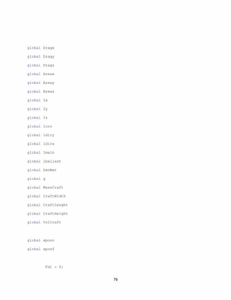
76

global Dragx

global Dragy

global Dragz

global Areax

global Areay

global Areaz

global Ix

global Iy

global Iz

global lcov

global ldiry

global ldirx

global lmain

global lballast

global DenWat

global g

global MassCraft

global CraftWidth

global CraftLenght

global CraftHeight

global VolCraft

global xposo

global xposf

Fd1 = 0;

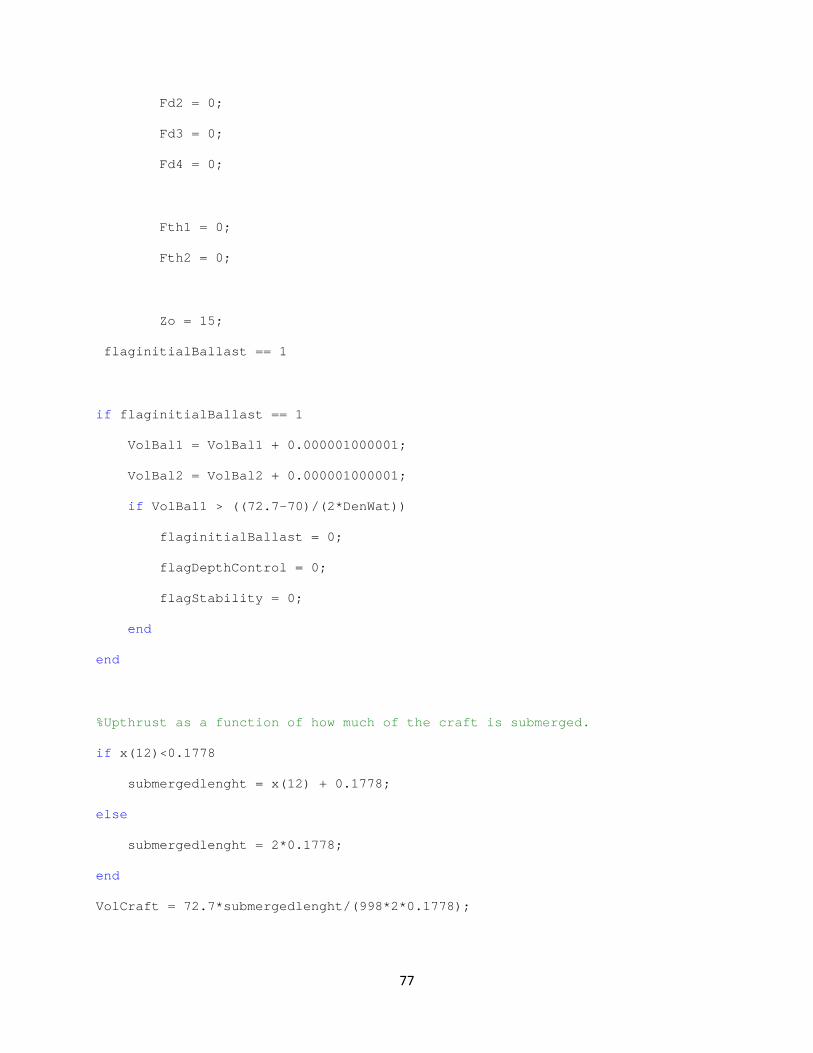
77

Fd2 = 0;

Fd3 = 0;

Fd4 = 0;

Fth1 = 0;

Fth2 = 0;

Zo = 15;

flaginitialBallast == 1

if flaginitialBallast == 1

VolBal1 = VolBal1 + 0.000001000001;

VolBal2 = VolBal2 + 0.000001000001;

if VolBal1 > ((72.7-70)/(2*DenWat))

flaginitialBallast = 0;

flagDepthControl = 0;

flagStability = 0;

end

end

%Upthrust as a function of how much of the craft is submerged.

if x(12)<0.1778

submergedlenght = x(12) + 0.1778;

else

submergedlenght = 2*0.1778;

end

VolCraft = 72.7*submergedlenght/(998*2*0.1778);

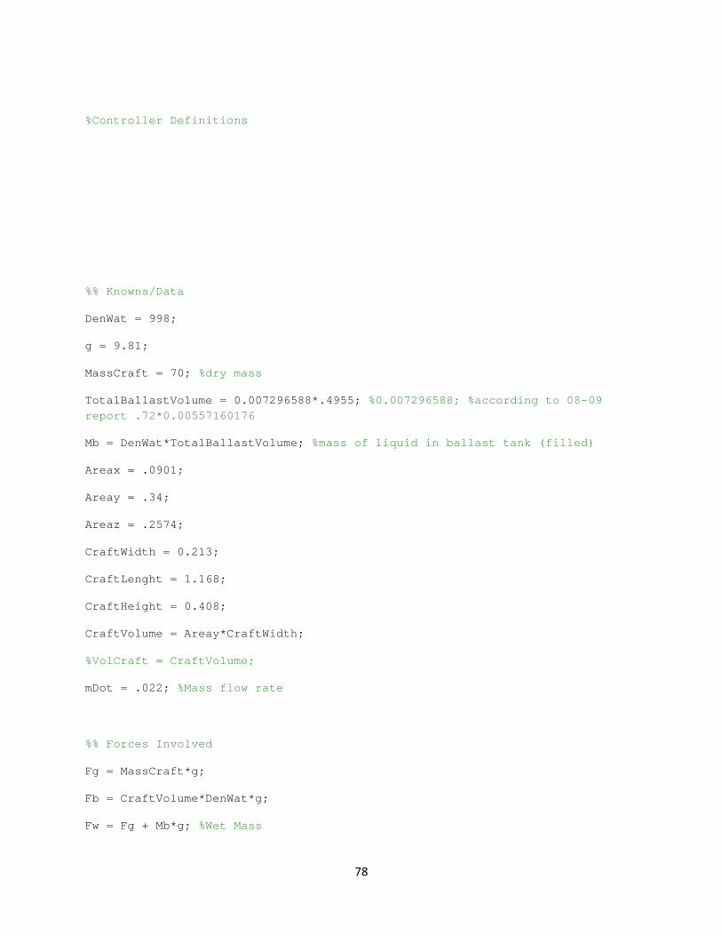
78

%Controller Definitions

%% Knowns/Data

DenWat = 998;

g = 9.81;

MassCraft = 70; %dry mass

TotalBallastVolume = 0.007296588*.4955; %0.007296588; %according to 08-09 report .72*0.00557160176

Mb = DenWat*TotalBallastVolume; %mass of liquid in ballast tank (filled)

Areax = .0901;

Areay = .34;

Areaz = .2574;

CraftWidth = 0.213;

CraftLenght = 1.168;

CraftHeight = 0.408;

CraftVolume = Areay*CraftWidth;

%VolCraft = CraftVolume;

mDot = .022; %Mass flow rate

%% Forces Involved

Fg = MassCraft*g;

Fb = CraftVolume*DenWat*g;

Fw = Fg + Mb*g; %Wet Mass

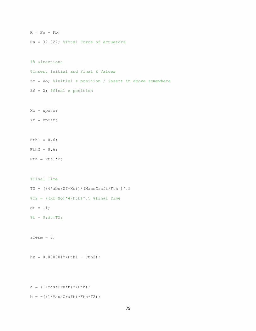
79

R = Fw - Fb;

Fa = 32.027; %Total Force of Actuators

%% Directions

%Insert Initial and Final Z Values

Zo = Zo; %initial z position / insert it above somewhere

Zf = 2; %final z position

Xo = xposo;

Xf = xposf;

Fth1 = 0.6;

Fth2 = 0.6;

Fth = Fth1*2;

%Final Time

T2 = ((4*abs(Xf-Xo))*(MassCraft/Fth))^.5

%T2 = ((Xf-Xo)*4/Fth)^.5 %final Time

dt = .1;

%t = 0:dt:T2;

zTerm = 0;

hx = 0.000001*(Fth1 - Fth2);

a = (1/MassCraft)*(Fth);

b = -((1/MassCraft)*Fth*T2);

80

c = ((1/(2*MassCraft))*Fth*(T2^2)+Xo-Xf);

T3 = (-b+(((b^2)-4*a*c)^.5))/(2*a);

T4 = (-b-(((b^2)-4*a*c)^.5))/(2*a);

T3=abs(T3);

T4=abs(T4);

if(0<=T3 && T3<=T2)

T1=T3;

else

T1=T4;

end

T1 = T2/2

%Time to change stage 1

t1data = 0:dt:T1;

t2data = T1:dt:T2;

T0 = 0; %Time for sub to stabilize

81

%% Control Stages

if Xf > Xo

if t>=T0 && t<=T1+T0

%zforce = -mDot*g*(t)-Fa+R;

%actuators offline

Fd1 = 0;

Fd2 = 0;

Fd3 = 0;

Fd4 = 0;

%ballasts offline

zTerm = 0;

%- 0.5*DenWat*(x(3))*abs(x(3))*Dragz*Areaz);

%main thrusters online

Fth1 = 0.60;

Fth2 = 0.60;

xTerm = Fth1+Fth2;

%(1/MassCraft)*(Fth1+Fth2)*t;

flagDepthControl == 0;

82

else if t>=T1 && t<=T2

Fd1 = 0;

Fd2 = 0;

Fd3 = 0;

Fd4 = 0;

zTerm = 0;

%+mDot*g*T1);

%0.5*DenWat*(x(3))*abs(x(3))*Dragz*Areaz);

zforce = 0;

Fth1 = 0.6;

Fth2 = 0.6;

xTerm = -Fth1 - Fth2;

else

Fd1 = 0;

Fd2 = 0;

Fd3 = 0;

Fd4 = 0;

zTerm = 0;

xTerm = 0;

Fth1 = 0;

Fth2 = 0;

end

83

end

end

if Xf <= Xo

if t>=T0 && t<=T1+T0

%zforce = -mDot*g*(t)-Fa+R;

%actuators offline

Fd1 = 0;

Fd2 = 0;

Fd3 = 0;

Fd4 = 0;

%ballasts offline

zTerm = 0;

%- 0.5*DenWat*(x(3))*abs(x(3))*Dragz*Areaz);

%main thrusters online

Fth1 = 0.60;

Fth2 = 0.60;

xTerm = -Fth1-Fth2;

%(1/MassCraft)*(Fth1+Fth2)*t;

flagDepthControl == 0;

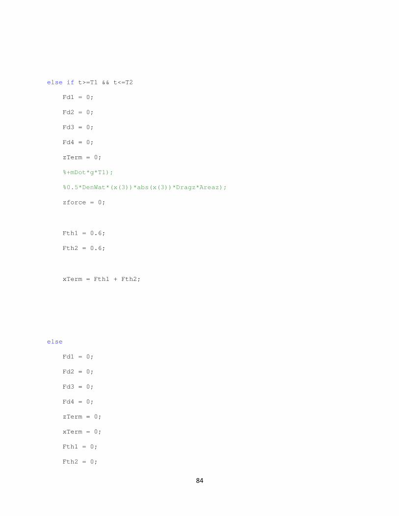
84

else if t>=T1 && t<=T2

Fd1 = 0;

Fd2 = 0;

Fd3 = 0;

Fd4 = 0;

zTerm = 0;

%+mDot*g*T1);

%0.5*DenWat*(x(3))*abs(x(3))*Dragz*Areaz);

zforce = 0;

Fth1 = 0.6;

Fth2 = 0.6;

xTerm = Fth1 + Fth2;

else

Fd1 = 0;

Fd2 = 0;

Fd3 = 0;

Fd4 = 0;

zTerm = 0;

xTerm = 0;

Fth1 = 0;

Fth2 = 0;

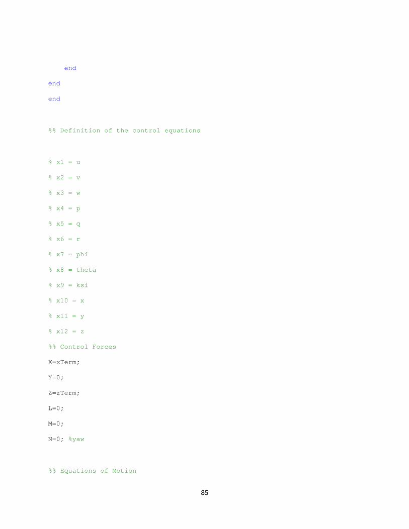
85

end

end

end

%% Definition of the control equations

% x1 = u

% x2 = v

% x3 = w

% x4 = p

% x5 = q

% x6 = r

% x7 = phi

% x8 = theta

% x9 = ksi

% x10 = x

% x11 = y

% x12 = z

%% Control Forces

X=xTerm;

Y=0;

Z=zTerm;

L=0;

M=0;

N=0; %yaw

%% Equations of Motion

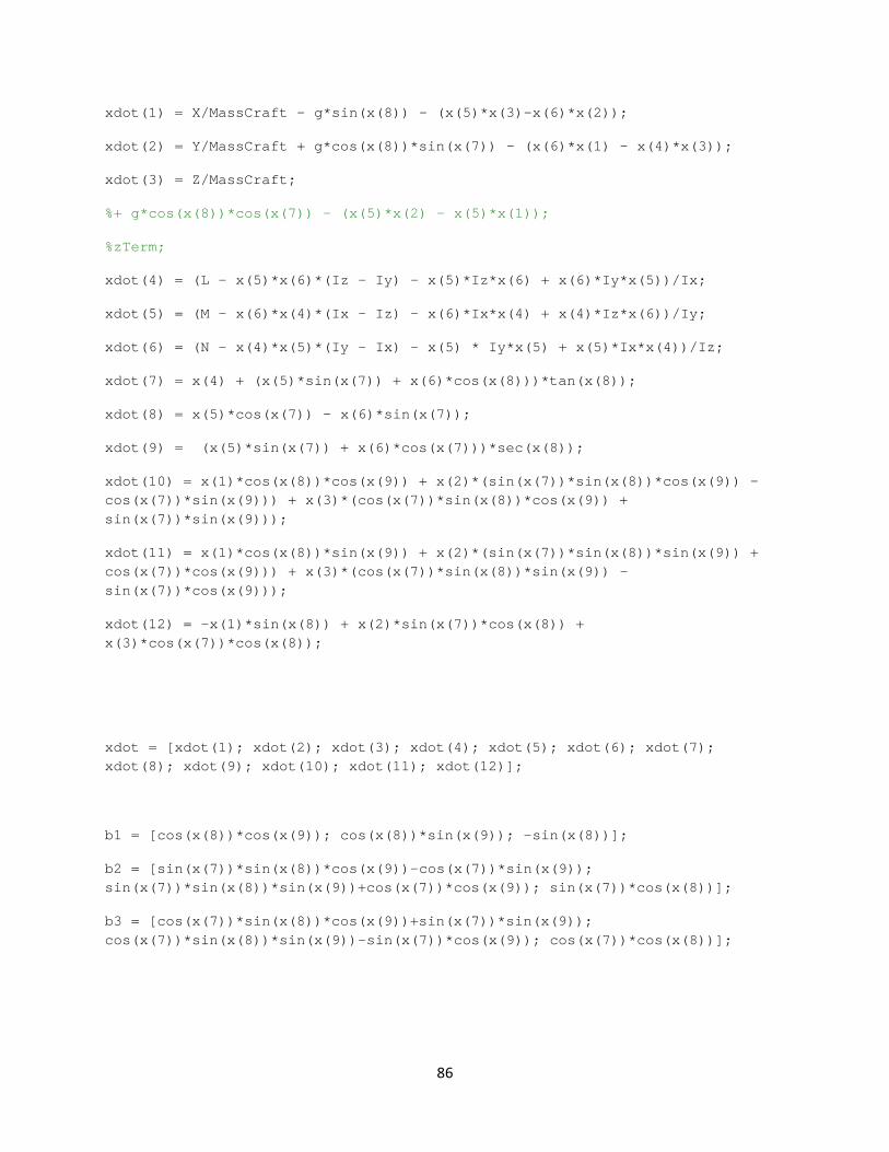
86

xdot(1) = X/MassCraft - g*sin(x(8)) - (x(5)*x(3)-x(6)*x(2));

xdot(2) = Y/MassCraft + g*cos(x(8))*sin(x(7)) - (x(6)*x(1) - x(4)*x(3));

xdot(3) = Z/MassCraft;

%+ g*cos(x(8))*cos(x(7)) - (x(5)*x(2) - x(5)*x(1));

%zTerm;

xdot(4) = (L - x(5)*x(6)*(Iz - Iy) - x(5)*Iz*x(6) + x(6)*Iy*x(5))/Ix;

xdot(5) = (M - x(6)*x(4)*(Ix - Iz) - x(6)*Ix*x(4) + x(4)*Iz*x(6))/Iy;

xdot(6) = (N - x(4)*x(5)*(Iy - Ix) - x(5) * Iy*x(5) + x(5)*Ix*x(4))/Iz;

xdot(7) = x(4) + (x(5)*sin(x(7)) + x(6)*cos(x(8)))*tan(x(8));

xdot(8) = x(5)*cos(x(7)) - x(6)*sin(x(7));

xdot(9) = (x(5)*sin(x(7)) + x(6)*cos(x(7)))*sec(x(8));

xdot(10) = x(1)*cos(x(8))*cos(x(9)) + x(2)*(sin(x(7))*sin(x(8))*cos(x(9)) - cos(x(7))*sin(x(9))) + x(3)*(cos(x(7))*sin(x(8))*cos(x(9)) + sin(x(7))*sin(x(9)));

xdot(11) = x(1)*cos(x(8))*sin(x(9)) + x(2)*(sin(x(7))*sin(x(8))*sin(x(9)) + cos(x(7))*cos(x(9))) + x(3)*(cos(x(7))*sin(x(8))*sin(x(9)) - sin(x(7))*cos(x(9)));

xdot(12) = -x(1)*sin(x(8)) + x(2)*sin(x(7))*cos(x(8)) + x(3)*cos(x(7))*cos(x(8));

xdot = [xdot(1); xdot(2); xdot(3); xdot(4); xdot(5); xdot(6); xdot(7); xdot(8); xdot(9); xdot(10); xdot(11); xdot(12)];

b1 = [cos(x(8))*cos(x(9)); cos(x(8))*sin(x(9)); -sin(x(8))];

b2 = [sin(x(7))*sin(x(8))*cos(x(9))-cos(x(7))*sin(x(9)); sin(x(7))*sin(x(8))*sin(x(9))+cos(x(7))*cos(x(9)); sin(x(7))*cos(x(8))];

b3 = [cos(x(7))*sin(x(8))*cos(x(9))+sin(x(7))*sin(x(9)); cos(x(7))*sin(x(8))*sin(x(9))-sin(x(7))*cos(x(9)); cos(x(7))*cos(x(8))];

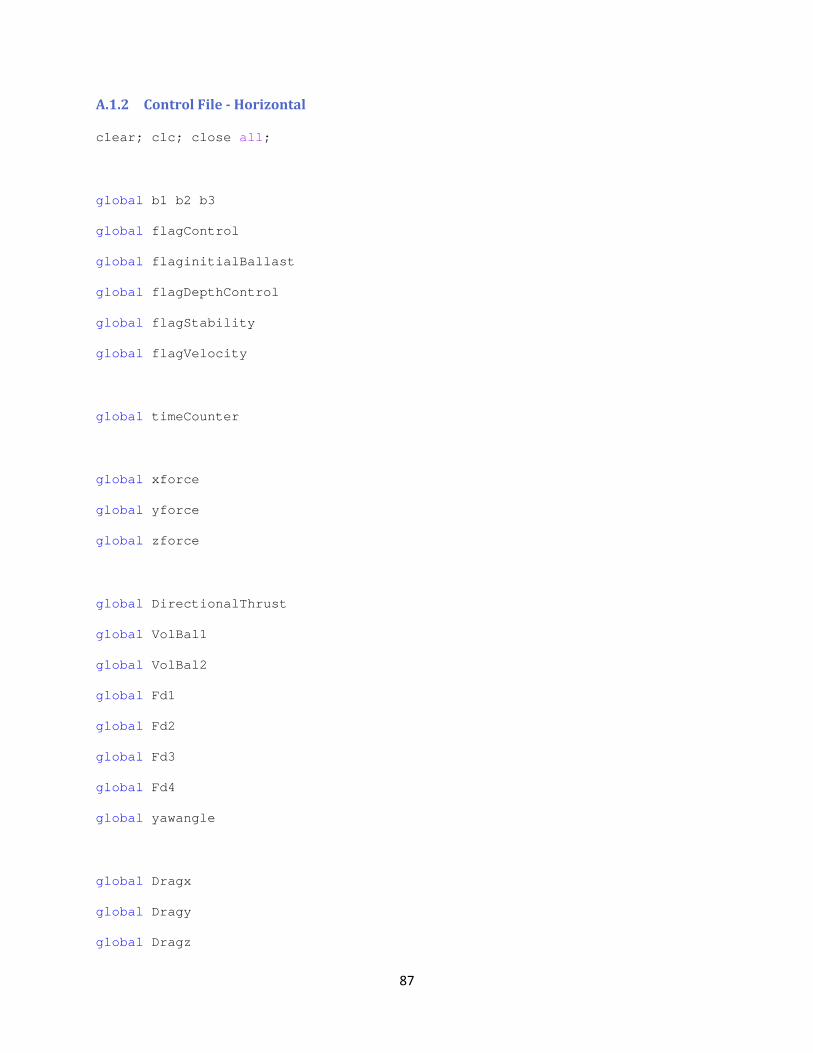
87

A.1.2 Control File - Horizontal

clear; clc; close all;

global b1 b2 b3

global flagControl

global flaginitialBallast

global flagDepthControl

global flagStability

global flagVelocity

global timeCounter

global xforce

global yforce

global zforce

global DirectionalThrust

global VolBal1

global VolBal2

global Fd1

global Fd2

global Fd3

global Fd4

global yawangle

global Dragx

global Dragy

global Dragz

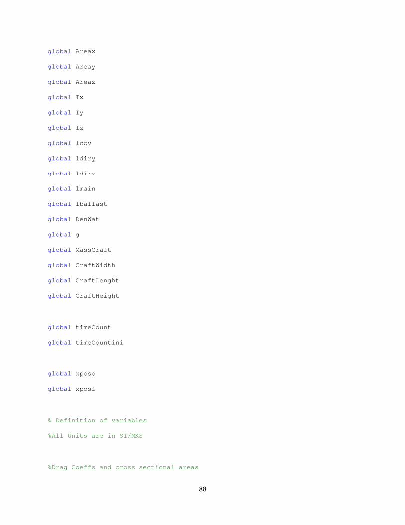
88

global Areax

global Areay

global Areaz

global Ix

global Iy

global Iz

global lcov

global ldiry

global ldirx

global lmain

global lballast

global DenWat

global g

global MassCraft

global CraftWidth

global CraftLenght

global CraftHeight

global timeCount

global timeCountini

global xposo

global xposf

% Definition of variables

%All Units are in SI/MKS

%Drag Coeffs and cross sectional areas

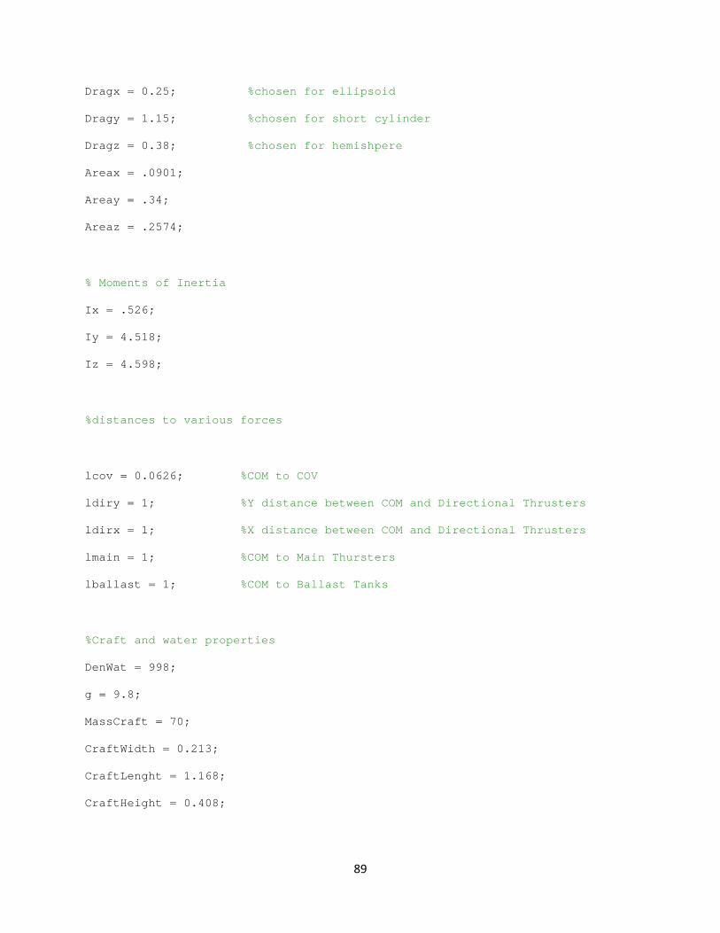
89

Dragx = 0.25; %chosen for ellipsoid

Dragy = 1.15; %chosen for short cylinder

Dragz = 0.38; %chosen for hemishpere

Areax = .0901;

Areay = .34;

Areaz = .2574;

% Moments of Inertia

Ix = .526;

Iy = 4.518;

Iz = 4.598;

%distances to various forces

lcov = 0.0626; %COM to COV

ldiry = 1; %Y distance between COM and Directional Thrusters

ldirx = 1; %X distance between COM and Directional Thrusters

lmain = 1; %COM to Main Thursters

lballast = 1; %COM to Ballast Tanks

%Craft and water properties

DenWat = 998;

g = 9.8;

MassCraft = 70;

CraftWidth = 0.213;

CraftLenght = 1.168;

CraftHeight = 0.408;

90

%Initiallization of Values

Fd1 = 0;

Fd2 = 0;

Fd3 = 0;

Fd4 = 0;

VolBal1 = 0;

VolBal2 = 0;

DirectionalThrust = [4 4 4 4];

timeCount = 0;

timeCountini = 0;

xforce = 0;

yforce = 0;

zforce = 0;

flagDepthControl = 0;

flagControl = 0;

flagStability = 0;

flaginitialBallast = 1;

flagVelocity = 0;

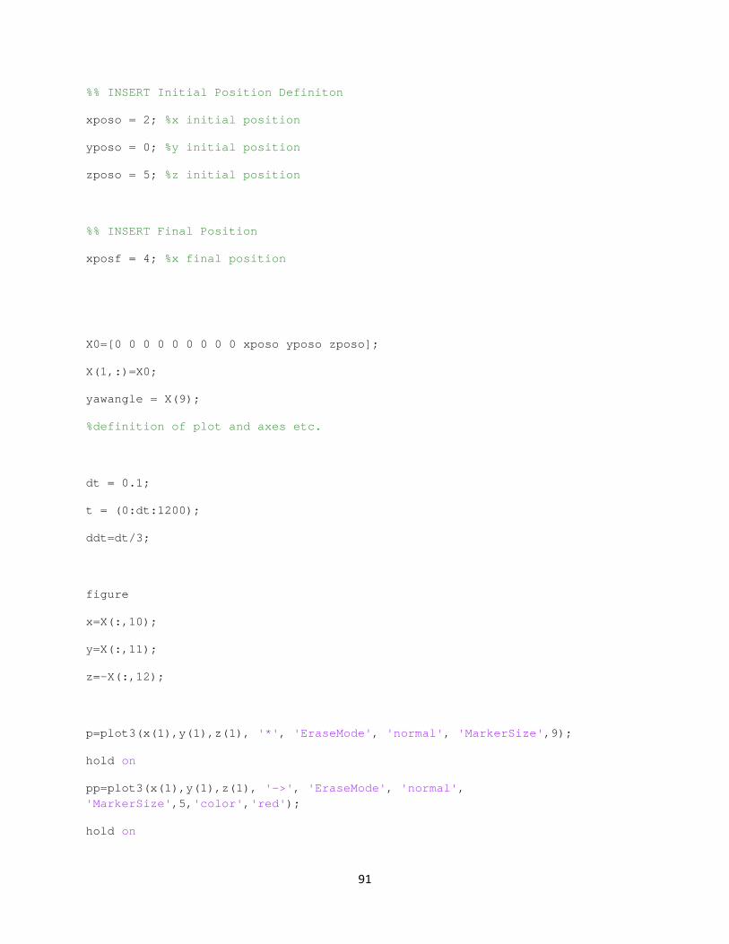
91

%% INSERT Initial Position Definiton

xposo = 2; %x initial position

yposo = 0; %y initial position

zposo = 5; %z initial position

%% INSERT Final Position

xposf = 4; %x final position

X0=[0 0 0 0 0 0 0 0 0 xposo yposo zposo];

X(1,:)=X0;

yawangle = X(9);

%definition of plot and axes etc.

dt = 0.1;

t = (0:dt:1200);

ddt=dt/3;

figure

x=X(:,10);

y=X(:,11);

z=-X(:,12);

p=plot3(x(1),y(1),z(1), '*', 'EraseMode', 'normal', 'MarkerSize',9);

hold on

pp=plot3(x(1),y(1),z(1), '->', 'EraseMode', 'normal', 'MarkerSize',5,'color','red');

hold on

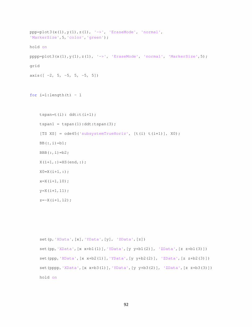
92

ppp=plot3(x(1),y(1),z(1), '->', 'EraseMode', 'normal', 'MarkerSize',5,'color','green');

hold on

pppp=plot3(x(1),y(1),z(1), '->', 'EraseMode', 'normal', 'MarkerSize',5);

grid

axis([ -2, 5, -5, 5, -5, 5])

for i=1:length(t) - 1

tspan=t(i): ddt:t(i+1);

tspan1 = tspan(1):ddt:tspan(3);

[TS XS] = ode45('subsystemTrueHoriz', [t(i) t(i+1)], X0);

BB(:,i)=b1;

BBB(:,i)=b2;

X(i+1,:)=XS(end,:);

X0=X(i+1,:);

x=X(i+1,10);

y=X(i+1,11);

z=-X(i+1,12);

set(p,'XData',[x],'YData',[y], 'ZData',[z])

set(pp,'XData',[x x+b1(1)],'YData',[y y+b1(2)], 'ZData',[z z+b1(3)])

set(ppp,'XData',[x x+b2(1)],'YData',[y y+b2(2)], 'ZData',[z z+b2(3)])

set(pppp,'XData',[x x+b3(1)],'YData',[y y+b3(2)], 'ZData',[z z+b3(3)])

hold on

93

title(['time=', num2str(t(i))]);

drawnow

%Mov(i) = getframe;

end

94

A.2 Yaw Maneuver

A.2.1 Subsystem File - Yaw

function [xdot] = subsystemTrueHoriz(t,x)

global Fd1

global Fd2

global Fd3

global Fd4

global VolBal1

global VolBal2

global yawangle

global ksio

global b1

global b2

global b3

global xforce

global yforce

global zforce

global DirectionalThrust

global flagControl

global flaginitialBallast

global flagDepthControl

global flagStability

global flagVelocity

95

global Dragx

global Dragy

global Dragz

global Areax

global Areay

global Areaz

global Ix

global Iy

global Iz

global lcov

global ldiry

global ldirx

global lmain

global lballast

global DenWat

global g

global MassCraft

global CraftWidth

global CraftLenght

global CraftHeight

global VolCraft

global ksiINT

%% Knowns/Data

DenWat = 998;

96

g = 9.81;

MassCraft = 72; %dry mass

TotalBallastVolume = 0.007296588*.4955; %0.007296588; %according to 08-09 report .72*0.00557160176

Mb = DenWat*TotalBallastVolume; %mass of liquid in ballast tank (filled)

Areax = .0901;

Areay = .34;

Areaz = .2574;

CraftWidth = 0.213;

CraftLenght = 1.168;

CraftHeight = 0.408;

CraftVolume = Areay*CraftWidth;

%VolCraft = CraftVolume;

mDot = .022; %Mass flow rate

%% Thrust of Craft

Fth1 = 1300;

Fth2 = 1300;

Ftht = Fth1 + Fth2; %Total Force

Torque = (CraftWidth/2)*Ftht %Total Torque

AngAccel = Torque*Areay/(Iz*MassCraft)

%% Forces Involved

Fg = MassCraft*g;

Fb = CraftVolume*DenWat*g;

Fw = Fg + Mb*g; %Wet Mass

R = Fw - Fb;

97

Fa = 32.027; %Total Force of Actuators

%% Directions

%Insert FINAL yaw orientation on ksiFIN

ksiFIN = 90; % HERE

%% Calculation

ksif = ksiFIN - ksiINT;

deltaKsi = abs(ksio-ksif)*pi/(180)

%% Total Trip Time

T2 = sqrt(2*deltaKsi/AngAccel);

T1 = T2/2; % First leg time

%% Control Stages

if ksiINT <= ksiFIN

if t>=0 && t<=T1

%actuators offline

Fd1 = 0;

Fd2 = 0;

Fd3 = 0;

Fd4 = 0;

%ballasts offline

zTerm = 0;

%main thrusters online

98

xTerm = 0;

yawTerm = .009457*Torque;

else if t>T1 && t<=T2

%actuators offline

Fd1 = 0;

Fd2 = 0;

Fd3 = 0;

Fd4 = 0;

%ballasts offline

zTerm = 0;

%main thrusters online

xTerm = 0;

yawTerm = -.009457*Torque;

else

Fd1 = 0;

Fd2 = 0;

Fd3 = 0;

Fd4 = 0;

zTerm = 0;

xTerm = 0;

yawTerm = 0;

end

end

99

end

if ksiINT > ksiFIN

if t>=0 && t<=T1

%actuators offline

Fd1 = 0;

Fd2 = 0;

Fd3 = 0;

Fd4 = 0;

%ballasts offline

zTerm = 0;

%main thrusters online

xTerm = 0;

yawTerm = -.009457*Torque;

else if t>T1 && t<=T2

%actuators offline

Fd1 = 0;

Fd2 = 0;

Fd3 = 0;

Fd4 = 0;

%ballasts offline

100

zTerm = 0;

%main thrusters online

xTerm = 0;

yawTerm = .009457*Torque;

else

Fd1 = 0;

Fd2 = 0;

Fd3 = 0;

Fd4 = 0;

zTerm = 0;

xTerm = 0;

yawTerm = 0;

end

end

end

%% Definition of the control equations

% x1 = u

% x2 = v

% x3 = w

% x4 = p

% x5 = q

% x6 = r

% x7 = phi

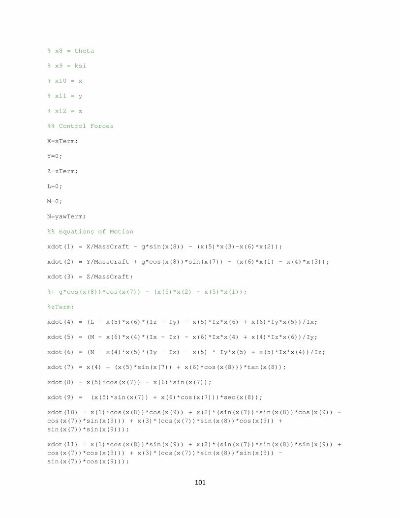
101

% x8 = theta

% x9 = ksi

% x10 = x

% x11 = y

% x12 = z

%% Control Forces

X=xTerm;

Y=0;

Z=zTerm;

L=0;

M=0;

N=yawTerm;

%% Equations of Motion

xdot(1) = X/MassCraft - g*sin(x(8)) - (x(5)*x(3)-x(6)*x(2));

xdot(2) = Y/MassCraft + g*cos(x(8))*sin(x(7)) - (x(6)*x(1) - x(4)*x(3));

xdot(3) = Z/MassCraft;

%+ g*cos(x(8))*cos(x(7)) - (x(5)*x(2) - x(5)*x(1));

%zTerm;

xdot(4) = (L - x(5)*x(6)*(Iz - Iy) - x(5)*Iz*x(6) + x(6)*Iy*x(5))/Ix;

xdot(5) = (M - x(6)*x(4)*(Ix - Iz) - x(6)*Ix*x(4) + x(4)*Iz*x(6))/Iy;

xdot(6) = (N - x(4)*x(5)*(Iy - Ix) - x(5) * Iy*x(5) + x(5)*Ix*x(4))/Iz;

xdot(7) = x(4) + (x(5)*sin(x(7)) + x(6)*cos(x(8)))*tan(x(8));

xdot(8) = x(5)*cos(x(7)) - x(6)*sin(x(7));

xdot(9) = (x(5)*sin(x(7)) + x(6)*cos(x(7)))*sec(x(8));

xdot(10) = x(1)*cos(x(8))*cos(x(9)) + x(2)*(sin(x(7))*sin(x(8))*cos(x(9)) - cos(x(7))*sin(x(9))) + x(3)*(cos(x(7))*sin(x(8))*cos(x(9)) + sin(x(7))*sin(x(9)));

xdot(11) = x(1)*cos(x(8))*sin(x(9)) + x(2)*(sin(x(7))*sin(x(8))*sin(x(9)) + cos(x(7))*cos(x(9))) + x(3)*(cos(x(7))*sin(x(8))*sin(x(9)) - sin(x(7))*cos(x(9)));

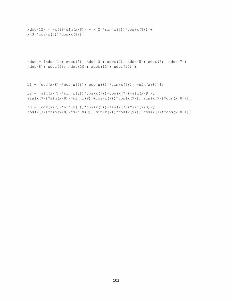
102

xdot(12) = -x(1)*sin(x(8)) + x(2)*sin(x(7))*cos(x(8)) + x(3)*cos(x(7))*cos(x(8));

xdot = [xdot(1); xdot(2); xdot(3); xdot(4); xdot(5); xdot(6); xdot(7); xdot(8); xdot(9); xdot(10); xdot(11); xdot(12)];

b1 = [cos(x(8))*cos(x(9)); cos(x(8))*sin(x(9)); -sin(x(8))];

b2 = [sin(x(7))*sin(x(8))*cos(x(9))-cos(x(7))*sin(x(9)); sin(x(7))*sin(x(8))*sin(x(9))+cos(x(7))*cos(x(9)); sin(x(7))*cos(x(8))];

b3 = [cos(x(7))*sin(x(8))*cos(x(9))+sin(x(7))*sin(x(9)); cos(x(7))*sin(x(8))*sin(x(9))-sin(x(7))*cos(x(9)); cos(x(7))*cos(x(8))];

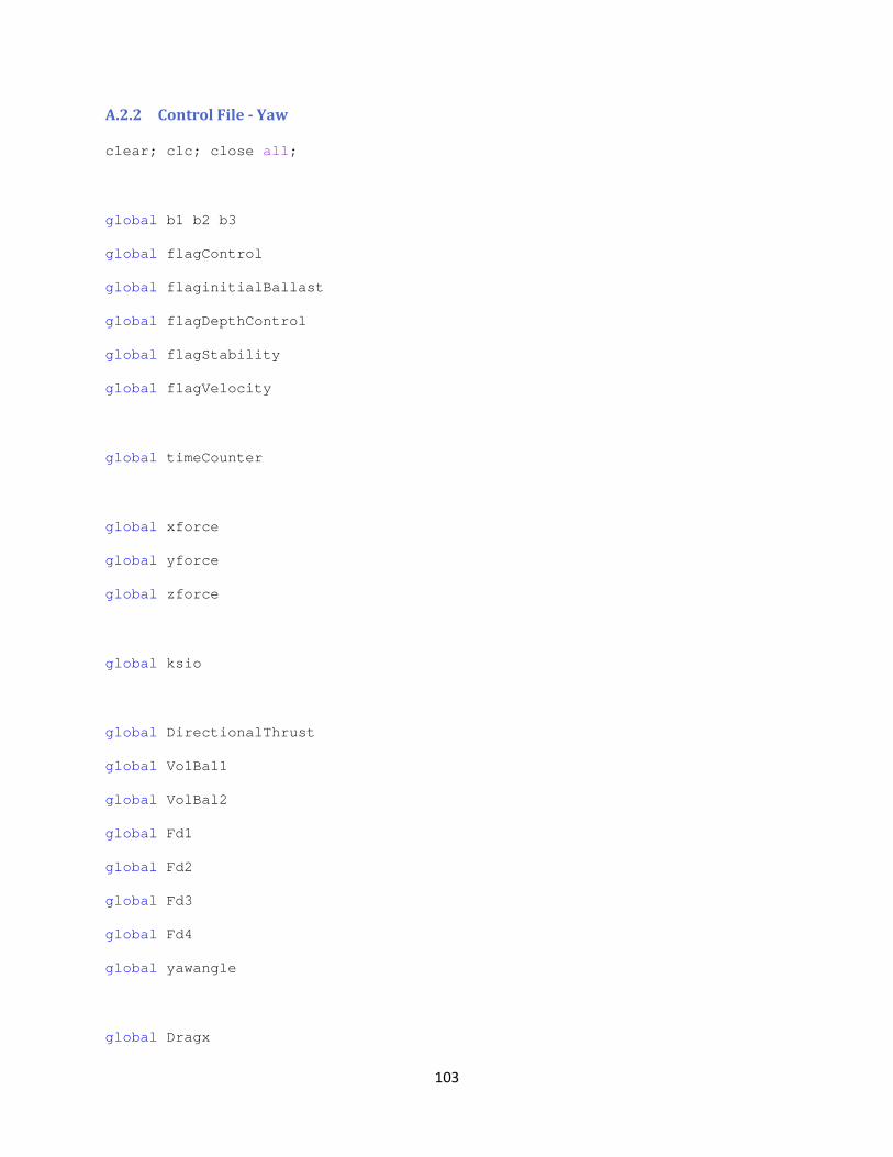
103

A.2.2 Control File - Yaw

clear; clc; close all;

global b1 b2 b3

global flagControl

global flaginitialBallast

global flagDepthControl

global flagStability

global flagVelocity

global timeCounter

global xforce

global yforce

global zforce

global ksio

global DirectionalThrust

global VolBal1

global VolBal2

global Fd1

global Fd2

global Fd3

global Fd4

global yawangle

global Dragx

104

global Dragy

global Dragz

global Areax

global Areay

global Areaz

global Ix

global Iy

global Iz

global lcov

global ldiry

global ldirx

global lmain

global lballast

global DenWat

global g

global MassCraft

global CraftWidth

global CraftLenght

global CraftHeight

global timeCount

global timeCountini

global ksiINT

% Definition of variables

%All Units are in SI/MKS

%Drag Coeffs and cross sectional areas

105

Dragx = 0.25; %chosen for ellipsoid

Dragy = 1.15; %chosen for short cylinder

Dragz = 0.38; %chosen for hemishpere

Areax = .0901;

Areay = .34;

Areaz = .2574;

% Moments of Inertia

Ix = .526;

Iy = 4.518;

Iz = 4.598;

%distances to various forces

lcov = 0.0626; %COM to COV

ldiry = 1; %Y distance between COM and Directional Thrusters

ldirx = 1; %X distance between COM and Directional Thrusters

lmain = 1; %COM to Main Thursters

lballast = 1; %COM to Ballast Tanks

%Craft and water properties

DenWat = 998;

g = 9.8;

MassCraft = 70;

CraftWidth = 0.213;

CraftLenght = 1.168;

CraftHeight = 0.408;

106

%Initiallization of Values

Fd1 = 0;

Fd2 = 0;

Fd3 = 0;

Fd4 = 0;

VolBal1 = 0;

VolBal2 = 0;

DirectionalThrust = [4 4 4 4];

timeCount = 0;

timeCountini = 0;

xforce = 0;

yforce = 0;

zforce = 0;

flagDepthControl = 0;

flagControl = 0;

flagStability = 0;

flaginitialBallast = 1;

flagVelocity = 0;

107

%% Insert Initial Position Definiton

xposo = 0; %x position

yposo = 0; %y position

zposo = 5; %z position

ksiINT = 0; %yaw orientation in degrees

%% Do not touch

ksio = ksiINT*pi/180; %yaw orientation

X0=[0 0 0 0 0 0 0 0 ksio xposo yposo zposo];

X(1,:)=X0;

yawangle = X(9);

%definition of plot and axes etc.

dt = 0.1;

t = (0:dt:1200);

ddt=dt/3;

figure

x=X(:,10);

y=X(:,11);

z=-X(:,12);

p=plot3(x(1),y(1),z(1), '*', 'EraseMode', 'normal', 'MarkerSize',5);

hold on

108

pp=plot3(x(1),y(1),z(1), '->', 'EraseMode', 'normal', 'MarkerSize',5, 'color','red');

hold on

ppp=plot3(x(1),y(1),z(1), '->', 'EraseMode', 'normal', 'MarkerSize',5,'color','green');

hold on

pppp=plot3(x(1),y(1),z(1), '->', 'EraseMode', 'normal', 'MarkerSize',5);

grid

axis([ -5, 5, -5, 5, -5, 5])

for i=1:length(t) - 1

tspan=t(i): ddt:t(i+1);

tspan1 = tspan(1):ddt:tspan(3);

[TS XS] = ode45('subsystemTrueYaw2', [t(i) t(i+1)], X0);

BB(:,i)=b1;

BBB(:,i)=b2;

X(i+1,:)=XS(end,:);

X0=X(i+1,:);

x=X(i+1,10);

y=X(i+1,11);

z=-X(i+1,12);

set(p,'XData',[x],'YData',[y], 'ZData',[z])

set(pp,'XData',[x x+b1(1)],'YData',[y y+b1(2)], 'ZData',[z z+b1(3)])

set(ppp,'XData',[x x+b2(1)],'YData',[y y+b2(2)], 'ZData',[z z+b2(3)])

set(pppp,'XData',[x x+b3(1)],'YData',[y y+b3(2)], 'ZData',[z z+b3(3)])

hold on

109

title(['time=', num2str(t(i))]);

drawnow

%Mov(i) = getframe;

end

110

A.3 Vertical Maneuver

A.3.1 Subsystem File – Vertical

function [xdot] = subsystemVERT(t,x)

global Fd1

global Fd2

global Fd3

global Fd4

global VolBal1

global VolBal2

global yawangle

global b1

global b2

global b3

global xforce

global yforce

global zforce

global DirectionalThrust

global flagControl

global flaginitialBallast

global flagDepthControl

global flagStability

global flagVelocity

global ksio

global xposo

111

global Dragx

global Dragy

global Dragz

global Areax

global Areay

global Areaz

global Ix

global Iy

global Iz

global lcov

global ldiry

global ldirx

global lmain

global lballast

global DenWat

global g

global MassCraft

global CraftWidth

global CraftLenght

global CraftHeight

global VolCraft

global FgNew

global MassCraftNewO

Fd1 = 0;

Fd2 = 0;

112

Fd3 = 0;

Fd4 = 0;

Fth1 = 0;

Fth2 = 0;

%% Knowns/Data

DenWat = 998;

g = 9.8066;

MassCraft = 72.275; %dry mass

TotalBallastVolume = 0.007296588*.4955; %0.007296588; %according to 08-09 report .72*0.00557160176

Mb = DenWat*TotalBallastVolume; %mass of liquid in ballast tank (filled)

Areax = .0901;

Areay = .34;

Areaz = .2574;

CraftWidth = 0.213;

CraftLenght = 1.168;

CraftHeight = 0.408;

CraftVolume = Areay*CraftWidth;

VolCraft = CraftVolume;

mDot = .022; %Mass flow rate

Vo = CraftVolume;

Po = 101325;

ZoINPUT = .2;

ZfINPUT = -.3;

113

Zo = 0.2264*(ZoINPUT^3)-0.8102*(ZoINPUT^2)+1.228*ZoINPUT;

Zf = ZfINPUT;%*.25

P1 = Po + DenWat*g*Zo;

P2 = P1 + DenWat*g*(Zf-Zo);

% Px*Vx=Py*Vy

V1 = (Po*Vo)/P1;

V2 = (P1*V1)/P2;

% Total mass required for neutral buoyancy at stated positions

MassTotalo = DenWat*V1;

MassTotalf = DenWat*V2;

% Mass of water to be filled in ballast tanks

FillInitial = MassTotalo - MassCraft;

FillFinal = MassTotalf - MassTotalo;

% Time required to fill tanks to achieve stated positions

To = FillInitial/mDot;

Tf = FillFinal/mDot;

114

Fboy=VolCraft*DenWat*g;

Tfill = 1; %fill tank for Tfill seconds

MassNewAssume = MassCraft + mDot*Tfill;

FgNewAssume = MassNewAssume*g;

ZForceAssume = FgNewAssume - Fboy;

AccelNewAssume = ZForceAssume/MassNewAssume;

TodAssume = (Zo/(.5*AccelNewAssume))^.5 %Total Travel time for descent

if t<Tfill

MassCraftNewO = MassCraft + mDot*t;

DenSub = MassCraftNewO/Vo;

FgNew = MassCraftNewO*g; %Force due to gravity

zTerm = (Zo*10/2.7211)*(FgNew - Fboy) %Force observed in the z direction

xTerm = 0;

end

if t<(TodAssume - Tfill) && t>=Tfill

zTerm = (Zo*10/2.7211)*(FgNew - Fboy)

xTerm = 0;

A=222222222222222

x(12)

end

if t>(TodAssume - Tfill) && t <= TodAssume

A = 555555555555555555

MassCraftNewOO = MassCraftNewO - mDot*(Tfill)

DenSub = MassCraftNewOO/Vo;

FgNew = MassCraftNewOO*g; %Force due to gravity

115

zTerm = (Zo*10/2.7211)*(FgNew - Fboy) %Force observed in the z direction

xTerm = 0;

end

if t > TodAssume

xTerm = 0;

zTerm = -.1;

end

%Resultant Propellor Torques Due to Main Thruster

hx = 0.000001*(Fth1 - Fth2); %Need to change to make it the angular momentum exhibited by the thrusters.

hx = 0;

xTerm = 0;

yawTerm=0;

% Definition of the control equations

% x1 = u

% x2 = v

% x3 = w

% x4 = p

% x5 = q

% x6 = r

% x7 = phi

% x8 = theta

% x9 = ksi

% x10 = x

116

% x11 = y

% x12 = z

%% Control Forces

X=xTerm;

Y=0;

Z=zTerm;

L=0;

M=0;

N=yawTerm;

%% Equations of Motion

xdot(1) = X/MassCraft - g*sin(x(8)) - (x(5)*x(3)-x(6)*x(2));

xdot(2) = Y/MassCraft + g*cos(x(8))*sin(x(7)) - (x(6)*x(1) - x(4)*x(3));

xdot(3) = Z/MassCraft;

%+ g*cos(x(8))*cos(x(7)) - (x(5)*x(2) - x(5)*x(1))-g

%zTerm;

xdot(4) = (L - x(5)*x(6)*(Iz - Iy) - x(5)*Iz*x(6) + x(6)*Iy*x(5))/Ix;

xdot(5) = (M - x(6)*x(4)*(Ix - Iz) - x(6)*Ix*x(4) + x(4)*Iz*x(6))/Iy;

xdot(6) = (N - x(4)*x(5)*(Iy - Ix) - x(5) * Iy*x(5) + x(5)*Ix*x(4))/Iz;

xdot(7) = x(4) + (x(5)*sin(x(7)) + x(6)*cos(x(8)))*tan(x(8));

xdot(8) = x(5)*cos(x(7)) - x(6)*sin(x(7));

xdot(9) = (x(5)*sin(x(7)) + x(6)*cos(x(7)))*sec(x(8));

xdot(10) = x(1)*cos(x(8))*cos(x(9)) + x(2)*(sin(x(7))*sin(x(8))*cos(x(9)) - cos(x(7))*sin(x(9))) + x(3)*(cos(x(7))*sin(x(8))*cos(x(9)) + sin(x(7))*sin(x(9)));

xdot(11) = x(1)*cos(x(8))*sin(x(9)) + x(2)*(sin(x(7))*sin(x(8))*sin(x(9)) + cos(x(7))*cos(x(9))) + x(3)*(cos(x(7))*sin(x(8))*sin(x(9)) - sin(x(7))*cos(x(9)));

xdot(12) = -x(1)*sin(x(8)) + x(2)*sin(x(7))*cos(x(8)) + x(3)*cos(x(7))*cos(x(8));

117

xdot = [xdot(1); xdot(2); xdot(3); xdot(4); xdot(5); xdot(6); xdot(7); xdot(8); xdot(9); xdot(10); xdot(11); xdot(12)];

b1 = [cos(x(8))*cos(x(9)); cos(x(8))*sin(x(9)); -sin(x(8))];

b2 = [sin(x(7))*sin(x(8))*cos(x(9))-cos(x(7))*sin(x(9)); sin(x(7))*sin(x(8))*sin(x(9))+cos(x(7))*cos(x(9)); sin(x(7))*cos(x(8))];

b3 = [cos(x(7))*sin(x(8))*cos(x(9))+sin(x(7))*sin(x(9)); cos(x(7))*sin(x(8))*sin(x(9))-sin(x(7))*cos(x(9)); cos(x(7))*cos(x(8))];

118

A.3.2 Control File – Vertical

clear; clc;

global b1 b2 b3

global flagControl

global flaginitialBallast

global flagDepthControl

global flagStability

global flagVelocity

global timeCounter

global xforce

global yforce

global zforce

global DirectionalThrust

global VolBal1

global VolBal2

global Fd1

global Fd2

global Fd3

global Fd4

global yawangle

global xposo

global Dragx

global Dragy

119

global Dragz

global Areax

global Areay

global Areaz

global Ix

global Iy

global Iz

global lcov

global ldiry

global ldirx

global lmain

global lballast

global DenWat

global g

global MassCraft

global CraftWidth

global CraftLenght

global CraftHeight

global timeCount

global timeCountini

% Definition of variables

%All Units are in SI/MKS

%Drag Coeffs and cross sectional areas

Dragx = 0.25; %chosen for ellipsoid

Dragy = 1.15; %chosen for short cylinder

120

Dragz = 0.38; %chosen for hemishpere

Areax = .0901;

Areay = .34;

Areaz = .2574;

% Moments of Inertia

Ix = .526;

Iy = 4.518;

Iz = 4.598;

%distances to various forces

lcov = 0.0626; %COM to COV

ldiry = 1; %Y distance between COM and Directional Thrusters

ldirx = 1; %X distance between COM and Directional Thrusters

lmain = 1; %COM to Main Thursters

lballast = 1; %COM to Ballast Tanks

%Craft and water properties

DenWat = 998;

g = 9.8066;

MassCraft = 72.2;

CraftWidth = 0.213;

CraftLenght = 1.168;

CraftHeight = 0.408;

%Initiallization of Values

Fd1 = 0;

121

Fd2 = 0;

Fd3 = 0;

Fd4 = 0;

VolBal1 = 0;

VolBal2 = 0;

DirectionalThrust = [4 4 4 4];

timeCount = 0;

timeCountini = 0;

xforce = 0;

yforce = 0;

zforce = 0;

flagDepthControl = 0;

flagControl = 0;

flagStability = 0;

flaginitialBallast = 1;

flagVelocity = 0;

%% Insert Initial Position

xposo = 0; %x position

yposo = 0; %y position

zposo = 0; %z position

ksio = 0; %initial yaw angle

%% Do Not Touch

X0=[0 0 0 0 0 0 0 0 ksio xposo yposo zposo];

122

X(1,:)=X0;

yawangle = X(9);

%definition of plot and axes etc.

dt = 0.1;

t = (0:dt:1200);

ddt=dt/3;

figure

x=X(:,10);

y=X(:,11);

z=-X(:,12);

set(gca, 'color','red')

%%set(gcf,'color',[0,0,0])

%%set(gca,'color','black',...)

p=plot3(x(1),y(1),z(1), '*', 'EraseMode', 'normal', 'MarkerSize',5,'color','black');

xlabel('meters')

hold on

pp=plot3(x(1),y(1),z(1), '->', 'EraseMode', 'normal', 'MarkerSize',5,'color','red');

ylabel('meters')

hold on

ppp=plot3(x(1),y(1),z(1), '->', 'EraseMode', 'normal', 'MarkerSize',5,'color','green');

zlabel('meters')

hold on

pppp=plot3(x(1),y(1),z(1), '->', 'EraseMode', 'normal', 'MarkerSize',5,'color','blue');

123

grid

hold on

% [A,B] = meshgrid(-3:.125:3);

% C = 0.00001*X;

% peaks(X,Y);

%

% meshz(A,B,C)

y = 0;

plot(x,y)

axis([ -4, 4, -4, 4, -2, 2])

for i=1:length(t) - 1

tspan=t(i): ddt:t(i+1);

tspan1 = tspan(1):ddt:tspan(3);

[TS XS] = ode45('subsystemVERT', [t(i) t(i+1)], X0);

BB(:,i)=b1;

BBB(:,i)=b2;

X(i+1,:)=XS(end,:);

X0=X(i+1,:);

x=X(i+1,10);

y=X(i+1,11);

z=-X(i+1,12);

set(p,'XData',[x],'YData',[y], 'ZData',[z])

124

set(pp,'XData',[x x+b1(1)],'YData',[y y+b1(2)], 'ZData',[z z+b1(3)])

set(ppp,'XData',[x x+b2(1)],'YData',[y y+b2(2)], 'ZData',[z z+b2(3)])

set(pppp,'XData',[x x+b3(1)],'YData',[y y+b3(2)], 'ZData',[z z+b3(3)])

hold on

title(['time=', num2str(t(i))]);

drawnow

%Mov(i) = getframe;

end

% movie2avi(Mov, 'DOF3')

125

A.4 Sample Mission

A.4.1 Subsystem File – Sample Mission

function [xdot] = subsystemMISSION(t,x)

global Fd1

global Fd2

global Fd3

global Fd4

global VolBal1

global VolBal2

global yawangle

global b1

global b2

global b3

global xforce

global yforce

global zforce

global DirectionalThrust

global flagControl

global flaginitialBallast

global flagDepthControl

global flagStability

global flagVelocity

global ksio

126

global xposo

global Dragx

global Dragy

global Dragz

global Areax

global Areay

global Areaz

global Ix

global Iy

global Iz

global lcov

global ldiry

global ldirx

global lmain

global lballast

global DenWat

global g

global MassCraft

global CraftWidth

global CraftLenght

global CraftHeight

global VolCraft

global FgNew

global MassCraftNewO

Fd1 = 0;

127

Fd2 = 0;

Fd3 = 0;

Fd4 = 0;

Fth1 = 0;

Fth2 = 0;

%% Knowns/Data

DenWat = 998;

g = 9.8066;

MassCraft = 72.275; %dry mass

TotalBallastVolume = 0.007296588*.4955; %0.007296588; %according to 08-09 report .72*0.00557160176

Mb = DenWat*TotalBallastVolume; %mass of liquid in ballast tank (filled)

Areax = .0901;

Areay = .34;

Areaz = .2574;

CraftWidth = 0.213;

CraftLenght = 1.168;

CraftHeight = 0.408;

CraftVolume = Areay*CraftWidth;

VolCraft = CraftVolume;

mDot = .022; %Mass flow rate

Vo = CraftVolume;

Po = 101325;

ZoINPUT = .2;

128

ZfINPUT = -.3;

Zo = 0.2264*(ZoINPUT^3)-0.8102*(ZoINPUT^2)+1.228*ZoINPUT;

Zf = ZfINPUT;%*.25

P1 = Po + DenWat*g*Zo;

P2 = P1 + DenWat*g*(Zf-Zo);

% Px*Vx=Py*Vy

V1 = (Po*Vo)/P1;

V2 = (P1*V1)/P2;

% Total mass required for neutral buoyancy at stated positions

MassTotalo = DenWat*V1;

MassTotalf = DenWat*V2;

% Mass of water to be filled in ballast tanks

FillInitial = MassTotalo - MassCraft;

FillFinal = MassTotalf - MassTotalo;

% Time required to fill tanks to achieve stated positions

To = FillInitial/mDot;

Tf = FillFinal/mDot;

129

Fboy=VolCraft*DenWat*g;

Tfill = 1; %fill tank for Tfill seconds

MassNewAssume = MassCraft + mDot*Tfill;

FgNewAssume = MassNewAssume*g;

ZForceAssume = FgNewAssume - Fboy;

AccelNewAssume = ZForceAssume/MassNewAssume;

TodAssume = (Zo/(.5*AccelNewAssume))^.5 %Total Travel time for descent

if t<Tfill

MassCraftNewO = MassCraft + mDot*t;

DenSub = MassCraftNewO/Vo;

FgNew = MassCraftNewO*g; %Force due to gravity

zTerm = (Zo*10/2.7211)*(FgNew - Fboy) %Force observed in the z direction

end

if t<(TodAssume - Tfill) && t>=Tfill

zTerm = (Zo*10/2.7211)*(FgNew - Fboy)

A=222222222222222

x(12)

end

if t>(TodAssume - Tfill) && t <= TodAssume

A = 555555555555555555

MassCraftNewOO = MassCraftNewO - mDot*(Tfill)

DenSub = MassCraftNewOO/Vo;

FgNew = MassCraftNewOO*g; %Force due to gravity

zTerm = (Zo*10/2.7211)*(FgNew - Fboy) %Force observed in the z direction

end

130

% if t > TodAssume

% zTerm = 0

% x(12)

% end

%% X DIR

Xo = xposo;

Xf = 1.5;

Fth1 = 0.6;

Fth2 = 0.6;

Fth = Fth1*2;

%Final Time

TxAssume = (4*(Xf-Xo)*(MassCraft/Fth))^.5;

%T4 = ((Xf-Xo)*4/Fth)^.5 %final Time

dt = .13;

Tx = TxAssume/2

xTerm=0;

if t >(TodAssume) && t<(Tx+TodAssume)

zTerm = -.15;

xTerm = Fth1 + Fth2

end

if t >=(Tx+TodAssume) && t<(TxAssume+TodAssume)

xTerm=-Fth1-Fth2;

131

zTerm = -.15;

end

% if t>=(TxAssume+TodAssume)

% xTerm=0;

% zTerm=0;

% end

%% Surface

if t>=(TxAssume+TodAssume) && x(12)>0.1

xTerm=0;

zTerm = -.15;

%-.1;

x(12)

end

if t>=(TxAssume+TodAssume) && x(12)<.1

xTerm=0;

zTerm = .15;

%-( g*cos(x(8))*cos(x(7)) - (x(5)*x(2) - x(5)*x(1))-g)*MassCraft;

x(12)

end

if t>=(TxAssume+TodAssume) && x(12)==0

xTerm=0;

zTerm=-.2;

end

% if t>=(TxAssume+TodAssume+2) && x(12)<0

% xTerm=0;

% zTerm=-2;

132

% x(12)

% end

% if x(12)<=0

% xTerm=0;

% zTerm=0;

% end

%Resultant Propellor Torques Due to Main Thruster

hx = 0.000001*(Fth1 - Fth2); %Need to change to make it the angular momentum exhibited by the thrusters.

hx = 0;

yawTerm=0;

% Definition of the control equations

% x1 = u

% x2 = v

% x3 = w

% x4 = p

% x5 = q

% x6 = r

% x7 = phi

% x8 = theta

% x9 = ksi

% x10 = x

133

% x11 = y

% x12 = z

%% Control Forces

X=xTerm;

Y=0;

Z=zTerm;

L=0;

M=0;

N=yawTerm;

%% Equations of Motion

xdot(1) = X/MassCraft - g*sin(x(8)) - (x(5)*x(3)-x(6)*x(2));

xdot(2) = Y/MassCraft + g*cos(x(8))*sin(x(7)) - (x(6)*x(1) - x(4)*x(3));

xdot(3) = Z/MassCraft;

%+ g*cos(x(8))*cos(x(7)) - (x(5)*x(2) - x(5)*x(1))-g

%zTerm;

xdot(4) = (L - x(5)*x(6)*(Iz - Iy) - x(5)*Iz*x(6) + x(6)*Iy*x(5))/Ix;

xdot(5) = (M - x(6)*x(4)*(Ix - Iz) - x(6)*Ix*x(4) + x(4)*Iz*x(6))/Iy;

xdot(6) = (N - x(4)*x(5)*(Iy - Ix) - x(5) * Iy*x(5) + x(5)*Ix*x(4))/Iz;

xdot(7) = x(4) + (x(5)*sin(x(7)) + x(6)*cos(x(8)))*tan(x(8));

xdot(8) = x(5)*cos(x(7)) - x(6)*sin(x(7));

xdot(9) = (x(5)*sin(x(7)) + x(6)*cos(x(7)))*sec(x(8));

xdot(10) = x(1)*cos(x(8))*cos(x(9)) + x(2)*(sin(x(7))*sin(x(8))*cos(x(9)) - cos(x(7))*sin(x(9))) + x(3)*(cos(x(7))*sin(x(8))*cos(x(9)) + sin(x(7))*sin(x(9)));

xdot(11) = x(1)*cos(x(8))*sin(x(9)) + x(2)*(sin(x(7))*sin(x(8))*sin(x(9)) + cos(x(7))*cos(x(9))) + x(3)*(cos(x(7))*sin(x(8))*sin(x(9)) - sin(x(7))*cos(x(9)));

xdot(12) = -x(1)*sin(x(8)) + x(2)*sin(x(7))*cos(x(8)) + x(3)*cos(x(7))*cos(x(8));

134

xdot = [xdot(1); xdot(2); xdot(3); xdot(4); xdot(5); xdot(6); xdot(7); xdot(8); xdot(9); xdot(10); xdot(11); xdot(12)];

b1 = [cos(x(8))*cos(x(9)); cos(x(8))*sin(x(9)); -sin(x(8))];

b2 = [sin(x(7))*sin(x(8))*cos(x(9))-cos(x(7))*sin(x(9)); sin(x(7))*sin(x(8))*sin(x(9))+cos(x(7))*cos(x(9)); sin(x(7))*cos(x(8))];

b3 = [cos(x(7))*sin(x(8))*cos(x(9))+sin(x(7))*sin(x(9)); cos(x(7))*sin(x(8))*sin(x(9))-sin(x(7))*cos(x(9)); cos(x(7))*cos(x(8))];

135

A.4.2 Control File – Sample Mission

clear; clc;

global b1 b2 b3

global flagControl

global flaginitialBallast

global flagDepthControl

global flagStability

global flagVelocity

global timeCounter

global xforce

global yforce

global zforce

global DirectionalThrust

global VolBal1

global VolBal2

global Fd1

global Fd2

global Fd3

global Fd4

global yawangle

global xposo

global Dragx

global Dragy

136

global Dragz

global Areax

global Areay

global Areaz

global Ix

global Iy

global Iz

global lcov

global ldiry

global ldirx

global lmain

global lballast

global DenWat

global g

global MassCraft

global CraftWidth

global CraftLenght

global CraftHeight

global timeCount

global timeCountini

% Definition of variables

%All Units are in SI/MKS

%Drag Coeffs and cross sectional areas

Dragx = 0.25; %chosen for ellipsoid

Dragy = 1.15; %chosen for short cylinder

137

Dragz = 0.38; %chosen for hemishpere

Areax = .0901;

Areay = .34;

Areaz = .2574;

% Moments of Inertia

Ix = .526;

Iy = 4.518;

Iz = 4.598;

%distances to various forces

lcov = 0.0626; %COM to COV

ldiry = 1; %Y distance between COM and Directional Thrusters

ldirx = 1; %X distance between COM and Directional Thrusters

lmain = 1; %COM to Main Thursters

lballast = 1; %COM to Ballast Tanks

%Craft and water properties

DenWat = 998;

g = 9.8066;

MassCraft = 72.2;

CraftWidth = 0.213;

CraftLenght = 1.168;

CraftHeight = 0.408;

%Initiallization of Values

Fd1 = 0;

Fd2 = 0;

138

Fd3 = 0;

Fd4 = 0;

VolBal1 = 0;

VolBal2 = 0;

DirectionalThrust = [4 4 4 4];

timeCount = 0;

timeCountini = 0;

xforce = 0;

yforce = 0;

zforce = 0;

flagDepthControl = 0;

flagControl = 0;

flagStability = 0;

flaginitialBallast = 1;

flagVelocity = 0;

%Initial Position Definiton

xposo = 0; %x position

yposo = 0; %y position

zposo = 0; %z position

ksio = 0; %initial yaw angle

X0=[0 0 0 0 0 0 0 0 ksio xposo yposo zposo];

X(1,:)=X0;

139

yawangle = X(9);

%definition of plot and axes etc.

dt = 0.1;

t = (0:dt:1200);

ddt=dt/3;

figure

x=X(:,10);

y=X(:,11);

z=-X(:,12);

set(gca, 'color','red')

%%set(gcf,'color',[0,0,0])

%%set(gca,'color','black',...)

p=plot3(x(1),y(1),z(1), '*', 'EraseMode', 'normal', 'MarkerSize',5,'color','black');

xlabel('meters')

hold on

pp=plot3(x(1),y(1),z(1), '->', 'EraseMode', 'normal', 'MarkerSize',5,'color','red');

ylabel('meters')

hold on

ppp=plot3(x(1),y(1),z(1), '->', 'EraseMode', 'normal', 'MarkerSize',5,'color','green');

zlabel('meters')

hold on

pppp=plot3(x(1),y(1),z(1), '->', 'EraseMode', 'normal', 'MarkerSize',5,'color','blue');

grid

140

hold on

% [A,B] = meshgrid(-3:.125:3);

% C = 0.00001*X;

% peaks(X,Y);

%

% meshz(A,B,C)

plot(x,y)

axis([ -4, 4, -4, 4, -2, 2])

for i=1:length(t) - 1

tspan=t(i): ddt:t(i+1);

tspan1 = tspan(1):ddt:tspan(3);

[TS XS] = ode45('subsystemMISSION', [t(i) t(i+1)], X0);

BB(:,i)=b1;

BBB(:,i)=b2;

X(i+1,:)=XS(end,:);

X0=X(i+1,:);

x=X(i+1,10);

y=X(i+1,11);

z=-X(i+1,12);

set(p,'XData',[x],'YData',[y], 'ZData',[z])

set(pp,'XData',[x x+b1(1)],'YData',[y y+b1(2)], 'ZData',[z z+b1(3)])

set(ppp,'XData',[x x+b2(1)],'YData',[y y+b2(2)], 'ZData',[z z+b2(3)])

set(pppp,'XData',[x x+b3(1)],'YData',[y y+b3(2)], 'ZData',[z z+b3(3)])

141

hold on

title(['time=', num2str(t(i))]);

drawnow

%Mov(i) = getframe;

end

% movie2avi(Mov, 'DOF3')

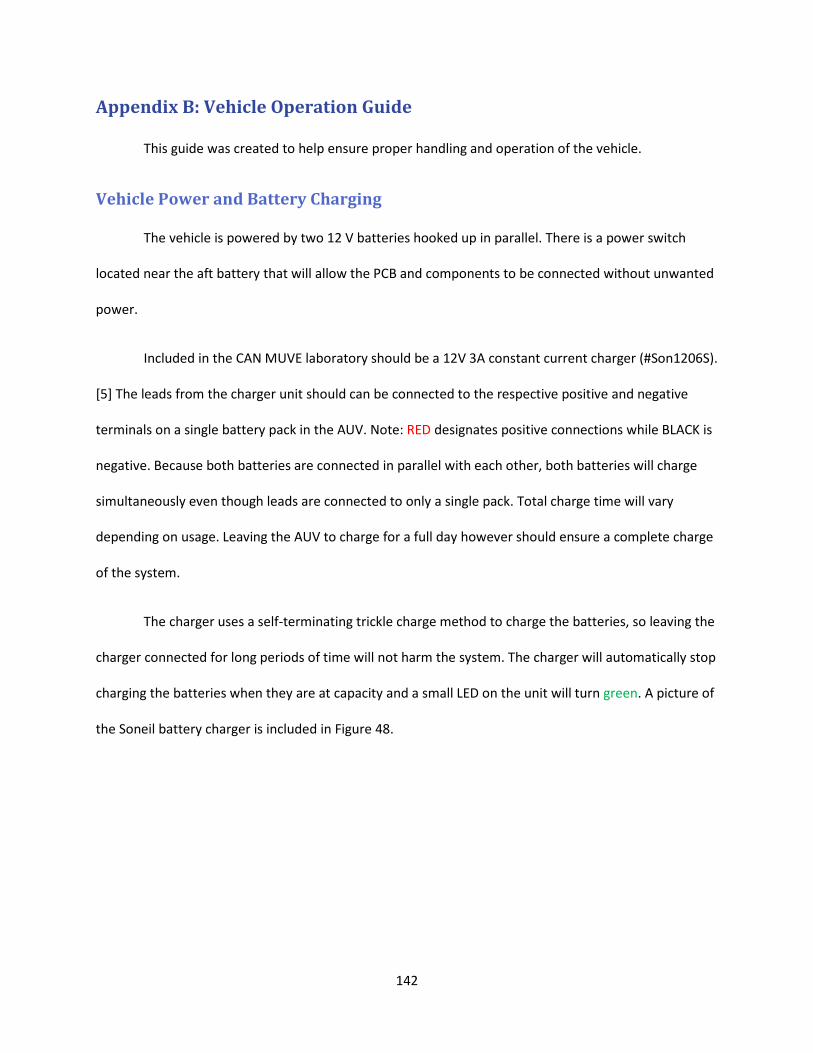
142

Appendix B: Vehicle Operation Guide

This guide was created to help ensure proper handling and operation of the vehicle.

Vehicle Power and Battery Charging

The vehicle is powered by two 12 V batteries hooked up in parallel. There is a power switch

located near the aft battery that will allow the PCB and components to be connected without unwanted

power.

Included in the CAN MUVE laboratory should be a 12V 3A constant current charger (#Son1206S).

[5] The leads from the charger unit should can be connected to the respective positive and negative

terminals on a single battery pack in the AUV. Note: RED designates positive connections while BLACK is

negative. Because both batteries are connected in parallel with each other, both batteries will charge

simultaneously even though leads are connected to only a single pack. Total charge time will vary

depending on usage. Leaving the AUV to charge for a full day however should ensure a complete charge

of the system.

The charger uses a self-terminating trickle charge method to charge the batteries, so leaving the

charger connected for long periods of time will not harm the system. The charger will automatically stop

charging the batteries when they are at capacity and a small LED on the unit will turn green. A picture of

the Soneil battery charger is included in Figure 48.

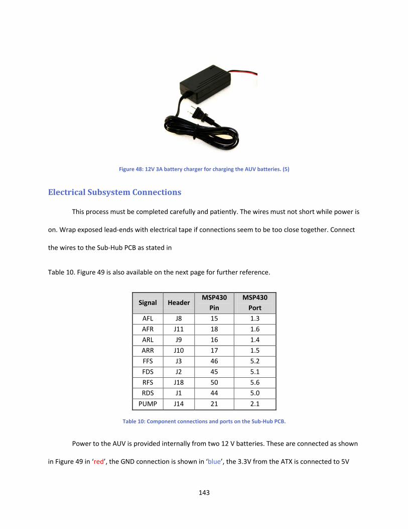
143

Figure 48: 12V 3A battery charger for charging the AUV batteries. (5)

Electrical Subsystem Connections

This process must be completed carefully and patiently. The wires must not short while power is

on. Wrap exposed lead-ends with electrical tape if connections seem to be too close together. Connect

the wires to the Sub-Hub PCB as stated in

Table 10. Figure 49 is also available on the next page for further reference.

Signal Header MSP430

Pin MSP430

Port

AFL J8 15 1.3

AFR J11 18 1.6

ARL J9 16 1.4

ARR J10 17 1.5

FFS J3 46 5.2

FDS J2 45 5.1

RFS J18 50 5.6

RDS J1 44 5.0

PUMP J14 21 2.1

Table 10: Component connections and ports on the Sub-Hub PCB.

Power to the AUV is provided internally from two 12 V batteries. These are connected as shown

in Figure 49 in ‘red’, the GND connection is shown in ‘blue’, the 3.3V from the ATX is connected to 5V

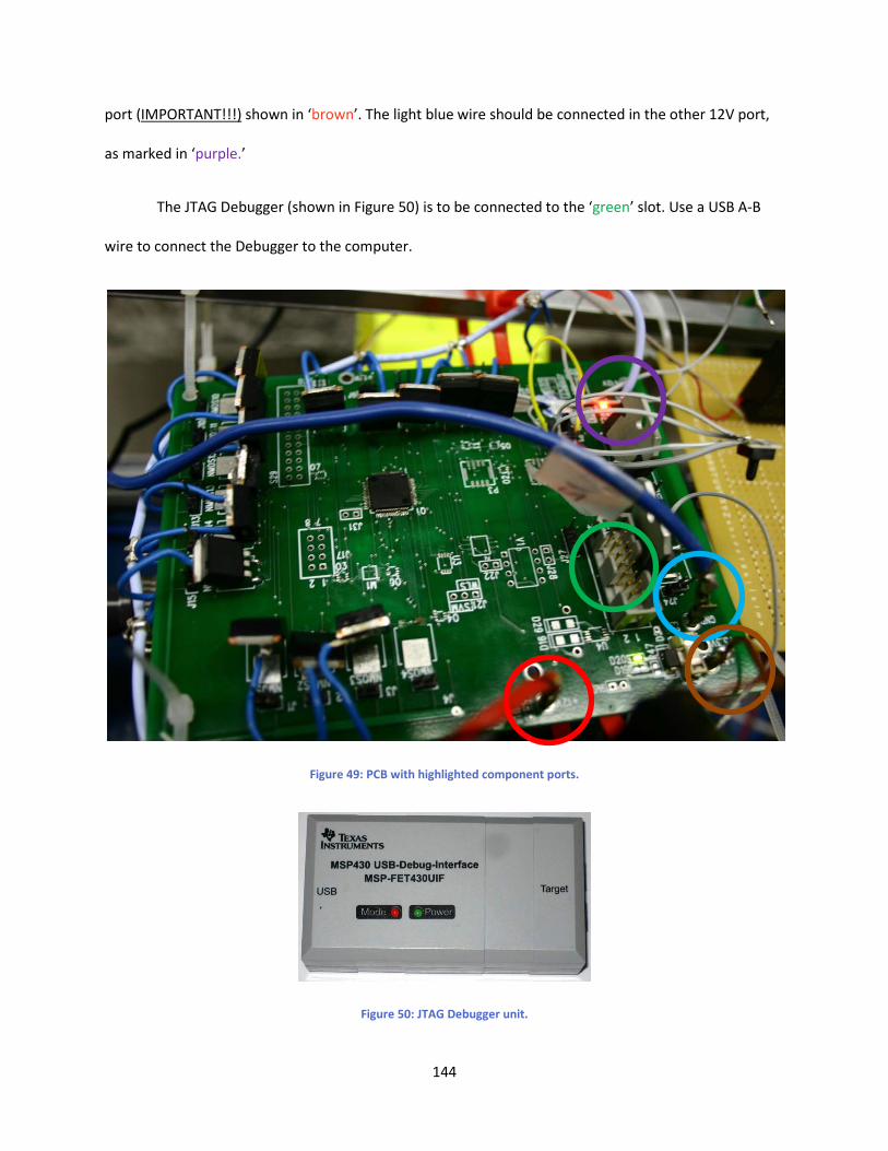
144

port (IMPORTANT!!!)

The JTAG Debugger (shown in

shown in ‘brown’. The light blue wire should be connected in the other 12V port,

as marked in ‘purple.’

Figure 50) is to be connected to the ‘green’ slot. Use a USB A-B

wire to connect the Debugger to the computer.

Figure 49: PCB with highlighted component ports.

Figure 50: JTAG Debugger unit.

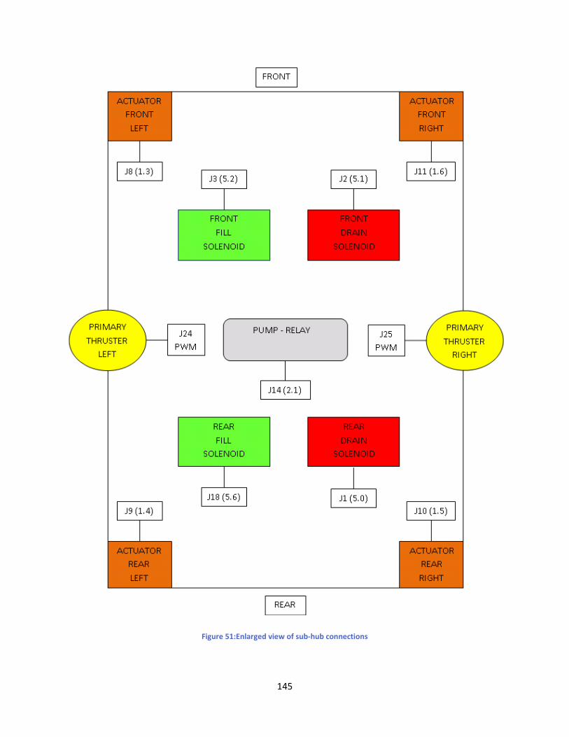
145

Figure 51:Enlarged view of sub-hub connections

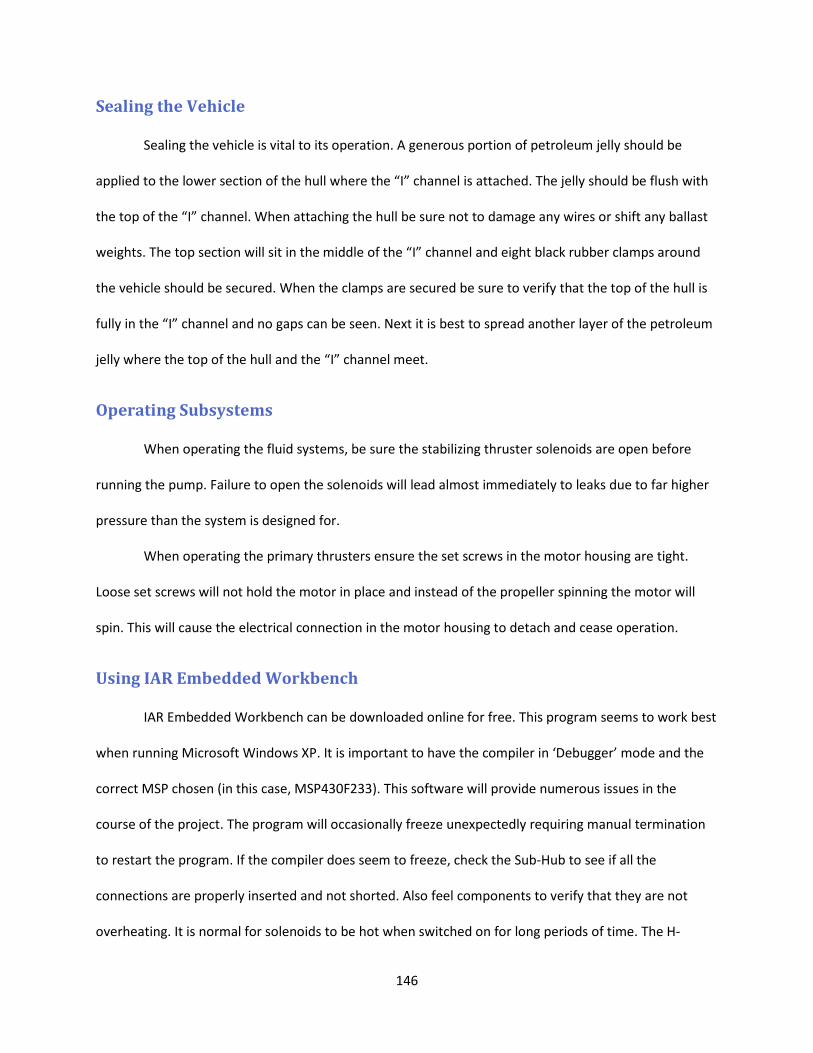
146

Sealing the Vehicle

Sealing the vehicle is vital to its operation. A generous portion of petroleum jelly should be

applied to the lower section of the hull where the “I” channel is attached. The jelly should be flush with

the top of the “I” channel. When attaching the hull be sure not to damage any wires or shift any ballast

weights. The top section will sit in the middle of the “I” channel and eight black rubber clamps around

the vehicle should be secured. When the clamps are secured be sure to verify that the top of the hull is

fully in the “I” channel and no gaps can be seen. Next it is best to spread another layer of the petroleum

jelly where the top of the hull and the “I” channel meet.

Operating Subsystems

When operating the fluid systems, be sure the stabilizing thruster solenoids are open before

running the pump. Failure to open the solenoids will lead almost immediately to leaks due to far higher

pressure than the system is designed for.

When operating the primary thrusters ensure the set screws in the motor housing are tight.

Loose set screws will not hold the motor in place and instead of the propeller spinning the motor will

spin. This will cause the electrical connection in the motor housing to detach and cease operation.

Using IAR Embedded Workbench

IAR Embedded Workbench can be downloaded online for free. This program seems to work best

when running Microsoft Windows XP. It is important to have the compiler in ‘Debugger’ mode and the

correct MSP chosen (in this case, MSP430F233). This software will provide numerous issues in the

course of the project. The program will occasionally freeze unexpectedly requiring manual termination

to restart the program. If the compiler does seem to freeze, check the Sub-Hub to see if all the

connections are properly inserted and not shorted. Also feel components to verify that they are not

overheating. It is normal for solenoids to be hot when switched on for long periods of time. The H-

147

Bridge units and the MOSFETs also tend to be warm while in use. The MSP unit must be cool at all times.

If any component seems to be abnormally hot, turn off the primary switch and re-check all connections.

Once checked, turn on the primary switch. It is normal for the vehicle’s systems to react

erratically upon re-boot. Next, open a workspace for a working program and run the compiler. The

erratic motion should cease.

Step through lines of code by clicking ‘Next Statement’ in the toolbar. Use the sample code

provided for testing purposes, available in Appendix C.1 System Check Code.

Transporting the Vehicle

Transporting the vehicle seems simple but if not done with caution can lead to severe damage

to various subsystems or the vehicle hull. A cart with wheels is used for transport. The vehicle sits in a

white platform constructed from PVC piping. The vehicle should be strapped down first to this platform,

using two green straps found in the lap, and then the platform should be strapped to the cart with a

yellow strap also found in the lab.

When wheeling the vehicle on the cart at least two people should be involved. One person will

push and steer the cart while the other helps avoid objects and prevent the vehicle from sliding if a strap

is not secured correctly. When transporting the vehicle from the cart to the test site only the yellow

strap should be removed. The white platform should remain attached to the vehicle and used to help

carry the vehicle. Removing the vehicle from the platform is the last step in transporting the vehicle.

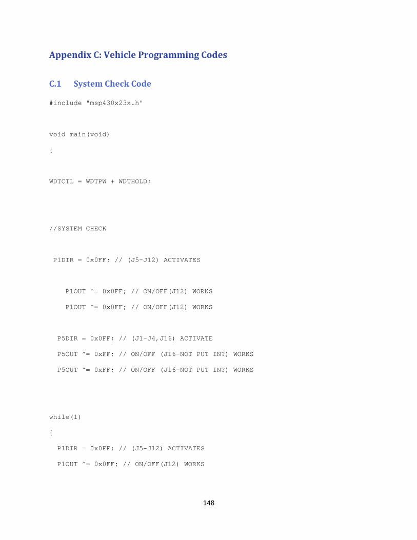
148

Appendix C: Vehicle Programming Codes

C.1 System Check Code

#include "msp430x23x.h"

void main(void)

{

WDTCTL = WDTPW + WDTHOLD;

//SYSTEM CHECK

P1DIR = 0x0FF; // (J5-J12) ACTIVATES

P1OUT ^= 0x0FF; // ON/OFF(J12) WORKS

P1OUT ^= 0x0FF; // ON/OFF(J12) WORKS

P5DIR = 0x0FF; // (J1-J4,J16) ACTIVATE

P5OUT ^= 0xFF; // ON/OFF (J16-NOT PUT IN?) WORKS

P5OUT ^= 0xFF; // ON/OFF (J16-NOT PUT IN?) WORKS

while(1)

{

P1DIR = 0x0FF; // (J5-J12) ACTIVATES

P1OUT ^= 0x0FF; // ON/OFF(J12) WORKS

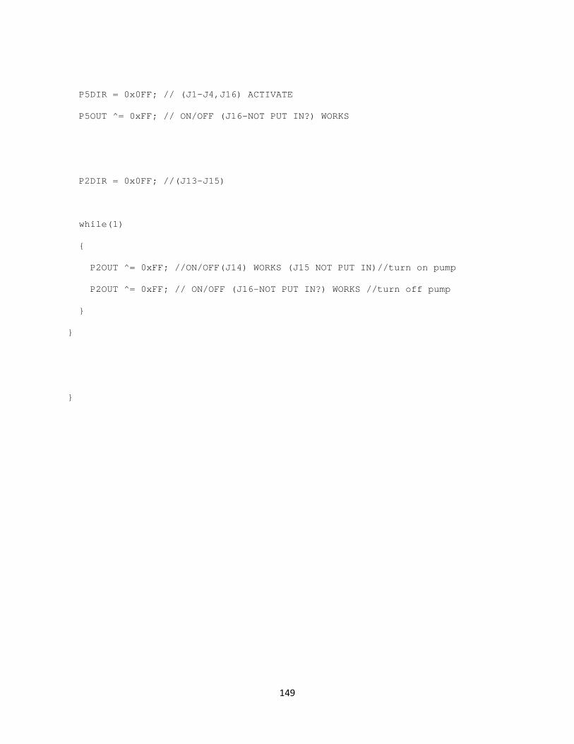
149

P5DIR = 0x0FF; // (J1-J4,J16) ACTIVATE

P5OUT ^= 0xFF; // ON/OFF (J16-NOT PUT IN?) WORKS

P2DIR = 0x0FF; //(J13-J15)

while(1)

{

P2OUT ^= 0xFF; //ON/OFF(J14) WORKS (J15 NOT PUT IN)//turn on pump

P2OUT ^= 0xFF; // ON/OFF (J16-NOT PUT IN?) WORKS //turn off pump

}

}

}

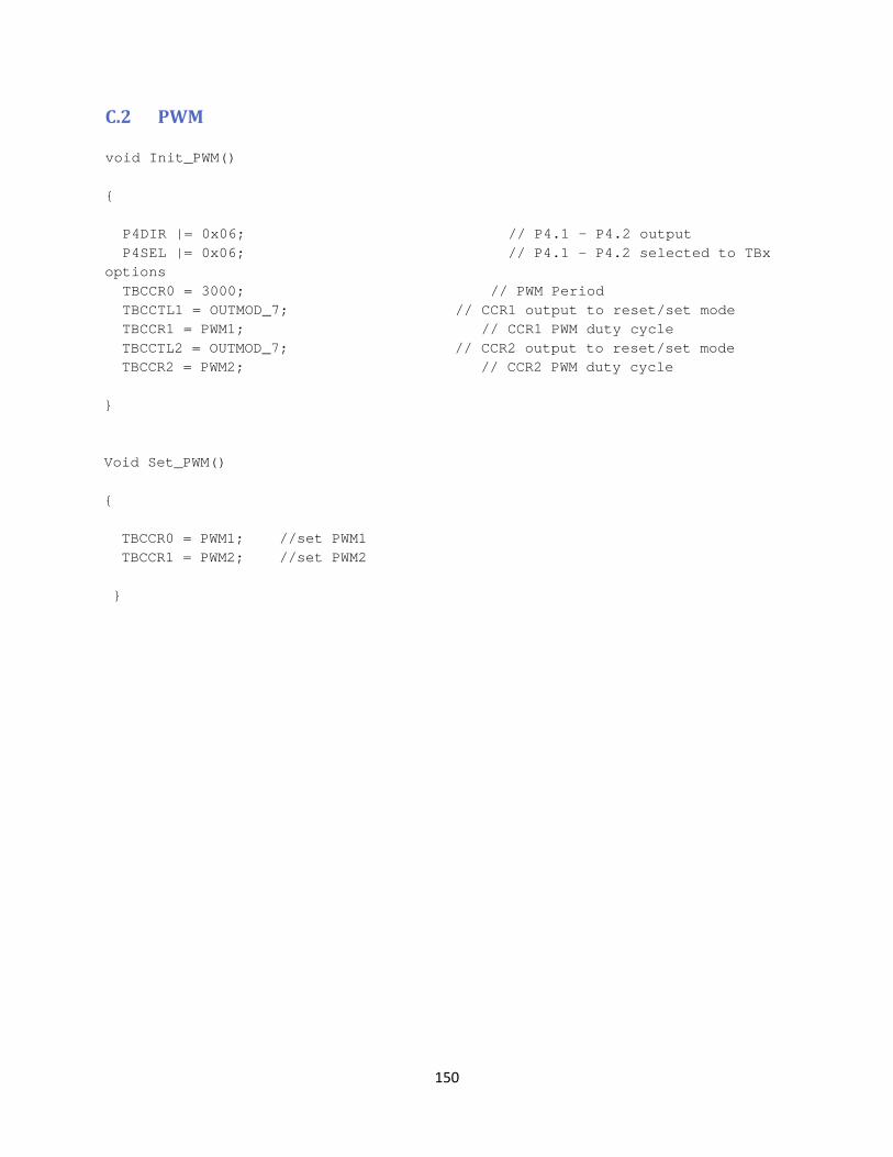
150

C.2 PWM

void Init_PWM() { P4DIR |= 0x06; // P4.1 - P4.2 output P4SEL |= 0x06; // P4.1 - P4.2 selected to TBx options TBCCR0 = 3000; // PWM Period TBCCTL1 = OUTMOD_7; // CCR1 output to reset/set mode TBCCR1 = PWM1; // CCR1 PWM duty cycle TBCCTL2 = OUTMOD_7; // CCR2 output to reset/set mode TBCCR2 = PWM2; // CCR2 PWM duty cycle } Void Set_PWM() { TBCCR0 = PWM1; //set PWM1 TBCCR1 = PWM2; //set PWM2 }

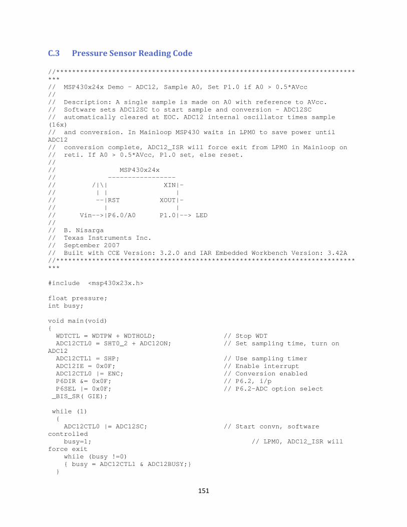
151

C.3 Pressure Sensor Reading Code

//****************************************************************************** // MSP430x24x Demo - ADC12, Sample A0, Set P1.0 if A0 > 0.5*AVcc // // Description: A single sample is made on A0 with reference to AVcc. // Software sets ADC12SC to start sample and conversion - ADC12SC // automatically cleared at EOC. ADC12 internal oscillator times sample (16x) // and conversion. In Mainloop MSP430 waits in LPM0 to save power until ADC12 // conversion complete, ADC12_ISR will force exit from LPM0 in Mainloop on // reti. If A0 > 0.5*AVcc, P1.0 set, else reset. // // MSP430x24x // ----------------- // /|\| XIN|- // | | | // --|RST XOUT|- // | | // Vin-->|P6.0/A0 P1.0|--> LED // // B. Nisarga // Texas Instruments Inc. // September 2007 // Built with CCE Version: 3.2.0 and IAR Embedded Workbench Version: 3.42A //****************************************************************************** #include <msp430x23x.h> float pressure; int busy; void main(void) { WDTCTL = WDTPW + WDTHOLD; // Stop WDT ADC12CTL0 = SHT0_2 + ADC12ON; // Set sampling time, turn on ADC12 ADC12CTL1 = SHP; // Use sampling timer ADC12IE = 0x0F; // Enable interrupt ADC12CTL0 |= ENC; // Conversion enabled P6DIR &= 0x0F; // P6.2, i/p P6SEL |= 0x0F; // P6.2-ADC option select _BIS_SR( GIE); while (1) { ADC12CTL0 |= ADC12SC; // Start convn, software controlled busy=1; // LPM0, ADC12_ISR will force exit while (busy !=0) { busy = ADC12CTL1 & ADC12BUSY;} }

152

} // ADC12 interrupt service routine #pragma vector=ADC12_VECTOR __interrupt void ADC12_ISR (void) { pressure = ADC12MEM2; }

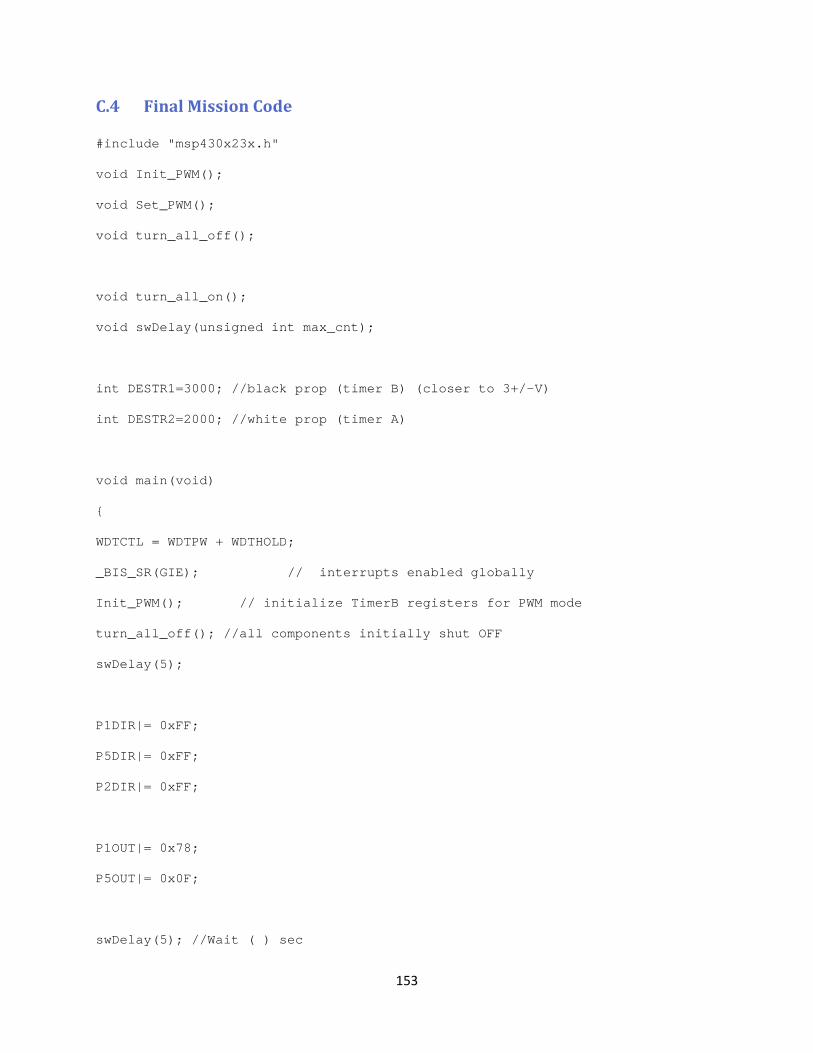
153

C.4 Final Mission Code

#include "msp430x23x.h"

void Init_PWM();

void Set_PWM();

void turn_all_off();

void turn_all_on();

void swDelay(unsigned int max_cnt);

int DESTR1=3000; //black prop (timer B) (closer to 3+/-V)

int DESTR2=2000; //white prop (timer A)

void main(void)

{

WDTCTL = WDTPW + WDTHOLD;

_BIS_SR(GIE); // interrupts enabled globally

Init_PWM(); // initialize TimerB registers for PWM mode

turn_all_off(); //all components initially shut OFF

swDelay(5);

P1DIR|= 0xFF;

P5DIR|= 0xFF;

P2DIR|= 0xFF;

P1OUT|= 0x78;

P5OUT|= 0x0F;

swDelay(5); //Wait ( ) sec

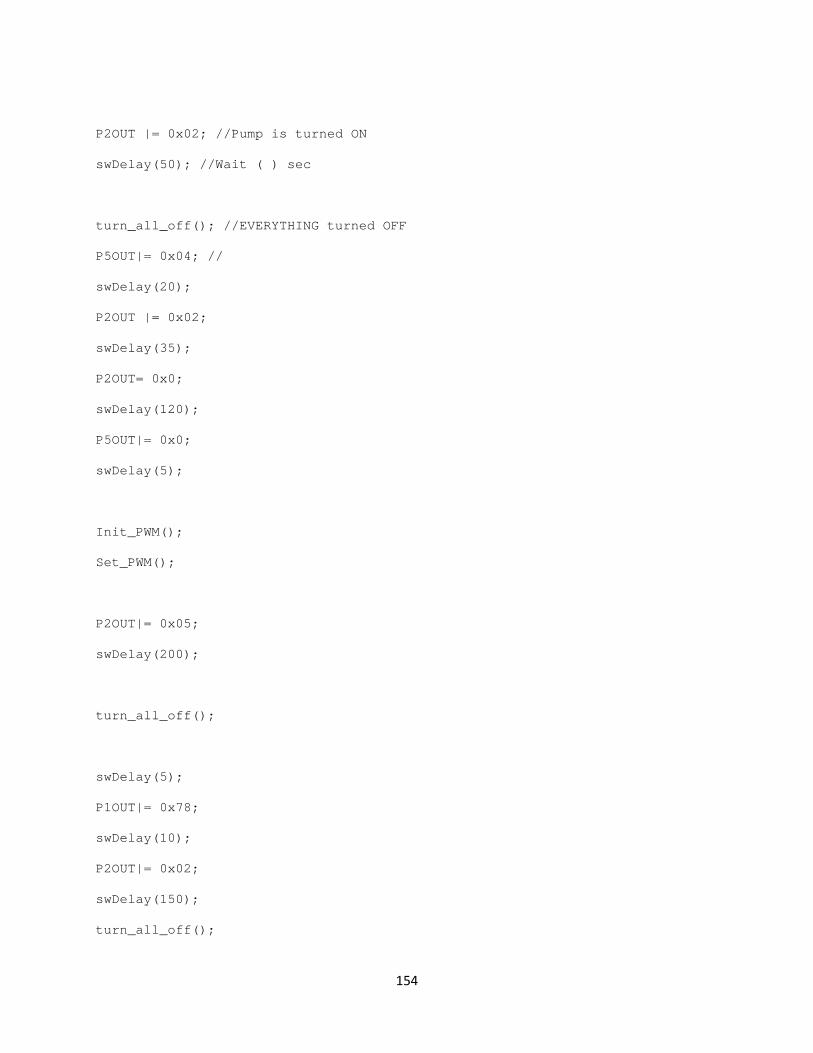
154

P2OUT |= 0x02; //Pump is turned ON

swDelay(50); //Wait ( ) sec

turn_all_off(); //EVERYTHING turned OFF

P5OUT|= 0x04; //

swDelay(20);

P2OUT |= 0x02;

swDelay(35);

P2OUT= 0x0;

swDelay(120);

P5OUT|= 0x0;

swDelay(5);

Init_PWM();

Set_PWM();

P2OUT|= 0x05;

swDelay(200);

turn_all_off();

swDelay(5);

P1OUT|= 0x78;

swDelay(10);

P2OUT|= 0x02;

swDelay(150);

turn_all_off();

155

}

void turn_all_off()

{

P1OUT = 0x0;

P2OUT = 0x0;

P5OUT = 0x0;

}

void Init_PWM()

{

P4DIR |= 0x06; // P4.1 - P4.2 output

P4SEL |= 0x06; // P4.1 - P4.2 selected to TBx options

TBCCR0 = 3000; // PWM Period

TBCCTL1 = OUTMOD_7; // CCR1 output to reset/set mode

TBCCR1 = DESTR1; // CCR1 PWM duty cycle

TBCCTL2 = OUTMOD_7; // CCR2 output to reset/set mode

TBCCR2 = DESTR2; // CCR2 PWM duty cycle

}

Void Set_PWM()

{

TBCCR0 = DESTR1; //set PWM1

TBCCR1 = DESTR2; //set PWM2

}

void swDelay(unsigned int max_cnt)

{

unsigned int cnt1=0, cnt2;

while (cnt1 < max_cnt)

{

156

cnt2 = 0;

while (cnt2 < 65535)

cnt2++;

cnt1++;

}

}

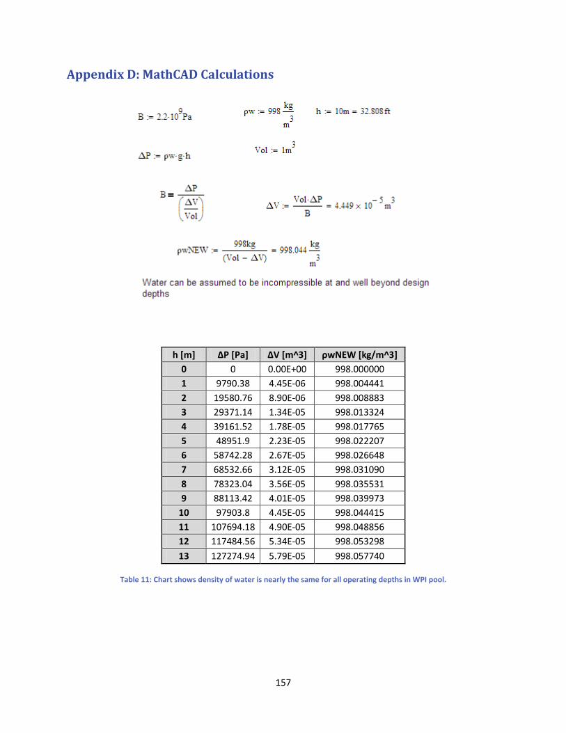
157

Appendix D: MathCAD Calculations

h [m] ΔP [Pa] ΔV [m^3] ρwNEW [kg/m^3] 0 0 0.00E+00 998.000000 1 9790.38 4.45E-06 998.004441 2 19580.76 8.90E-06 998.008883 3 29371.14 1.34E-05 998.013324 4 39161.52 1.78E-05 998.017765 5 48951.9 2.23E-05 998.022207 6 58742.28 2.67E-05 998.026648 7 68532.66 3.12E-05 998.031090 8 78323.04 3.56E-05 998.035531 9 88113.42 4.01E-05 998.039973

10 97903.8 4.45E-05 998.044415 11 107694.18 4.90E-05 998.048856 12 117484.56 5.34E-05 998.053298

13 127274.94 5.79E-05 998.057740

Table 11: Chart shows density of water is nearly the same for all operating depths in WPI pool.

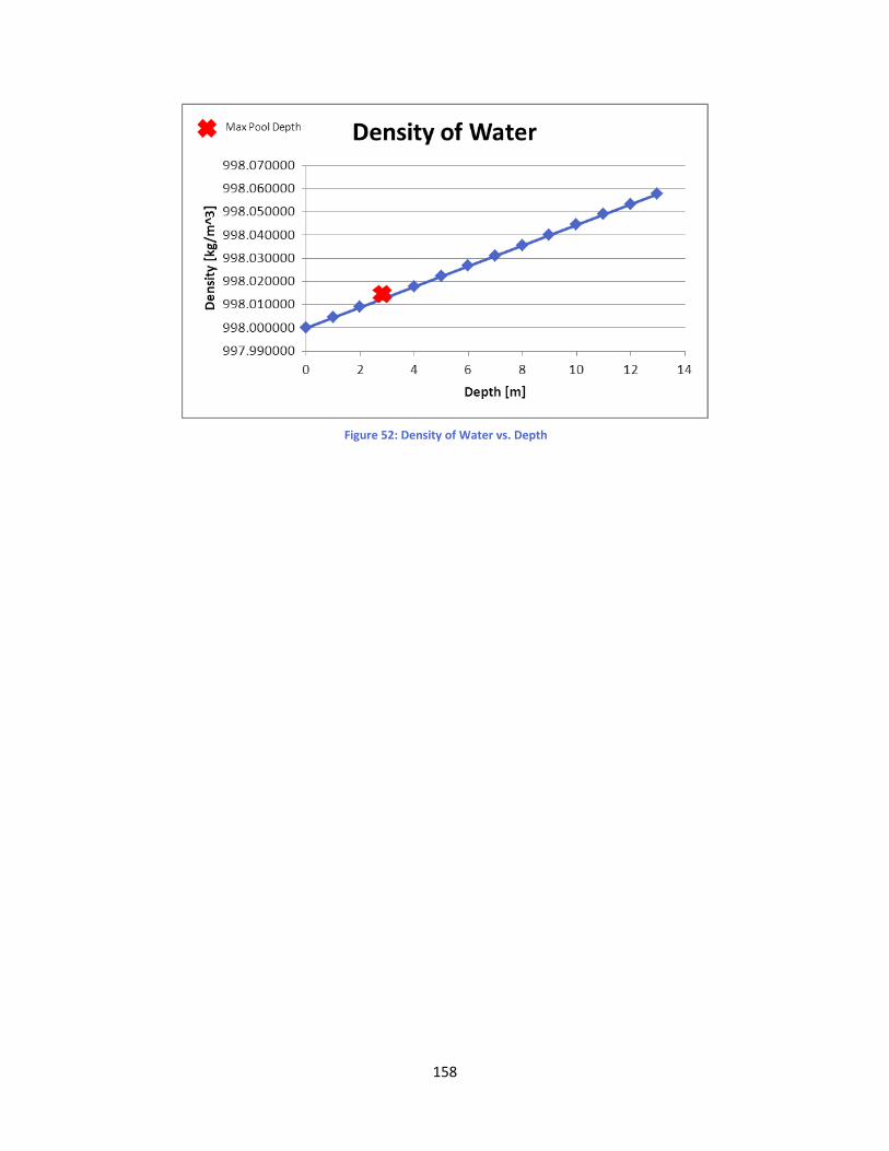
158

Figure 52: Density of Water vs. Depth

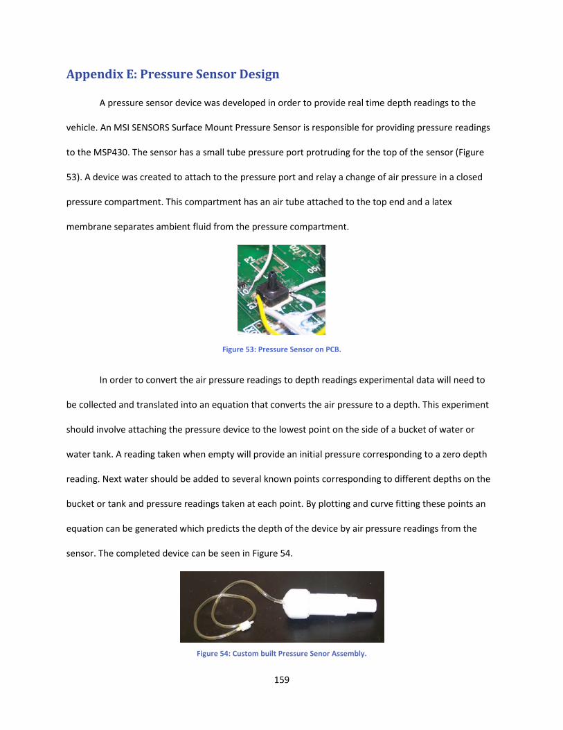
159

Appendix E: Pressure Sensor Design

A pressure sensor device was developed in order to provide real time depth readings to the

vehicle. An MSI SENSORS Surface Mount Pressure Sensor is responsible for providing pressure readings

to the MSP430. The sensor has a small tube pressure port protruding for the top of the sensor (Figure

53). A device was created to attach to the pressure port and relay a change of air pressure in a closed

pressure compartment. This compartment has an air tube attached to the top end and a latex

membrane separates ambient fluid from the pressure compartment.

Figure 53: Pressure Sensor on PCB.

In order to convert the air pressure readings to depth readings experimental data will need to

be collected and translated into an equation that converts the air pressure to a depth. This experiment

should involve attaching the pressure device to the lowest point on the side of a bucket of water or

water tank. A reading taken when empty will provide an initial pressure corresponding to a zero depth

reading. Next water should be added to several known points corresponding to different depths on the

bucket or tank and pressure readings taken at each point. By plotting and curve fitting these points an

equation can be generated which predicts the depth of the device by air pressure readings from the

sensor. The completed device can be seen in Figure 54.

Figure 54: Custom built Pressure Senor Assembly.

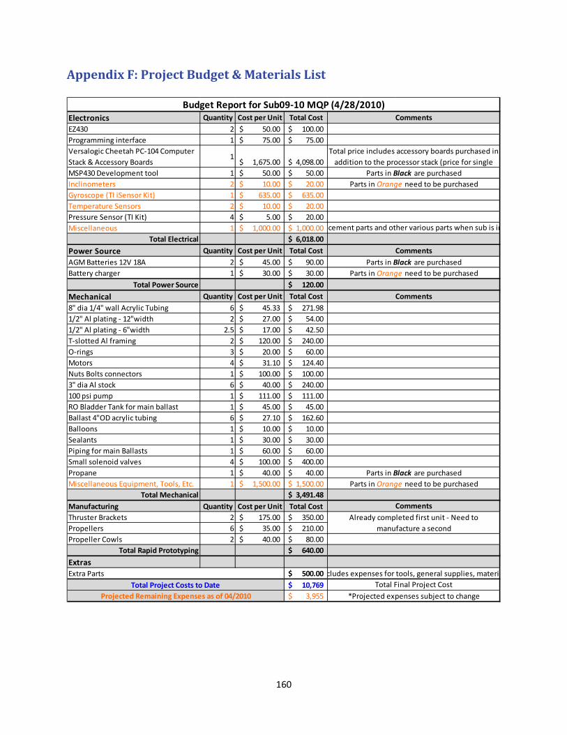
160

Appendix F: Project Budget & Materials List

Electronics Quantity Cost per Unit Total CostEZ430 2 50.00$ 100.00$ Programming interface 1 75.00$ 75.00$ Versalogic Cheetah PC-104 Computer Stack & Accessory Boards

11,675.00$ 4,098.00$

MSP430 Development tool 1 50.00$ 50.00$ Inclinometers 2 10.00$ 20.00$ Gyroscope (TI iSensor Kit) 1 635.00$ 635.00$ Temperature Sensors 2 10.00$ 20.00$ Pressure Sensor (TI Kit) 4 5.00$ 20.00$ Miscellaneous 1 1,000.00$ 1,000.00$

Total Electrical 6,018.00$

Power Source Quantity Cost per Unit Total CostAGM Batteries 12V 18A 2 45.00$ 90.00$ Battery charger 1 30.00$ 30.00$

Total Power Source 120.00$

Mechanical Quantity Cost per Unit Total Cost8" dia 1/4" wall Acrylic Tubing 6 45.33$ 271.98$ 1/2" Al plating - 12"width 2 27.00$ 54.00$ 1/2" Al plating - 6"width 2.5 17.00$ 42.50$ T-slotted Al framing 2 120.00$ 240.00$ O-rings 3 20.00$ 60.00$ Motors 4 31.10$ 124.40$ Nuts Bolts connectors 1 100.00$ 100.00$ 3" dia Al stock 6 40.00$ 240.00$ 100 psi pump 1 111.00$ 111.00$ RO Bladder Tank for main ballast 1 45.00$ 45.00$ Ballast 4"OD acrylic tubing 6 27.10$ 162.60$ Balloons 1 10.00$ 10.00$ Sealants 1 30.00$ 30.00$ Piping for main Ballasts 1 60.00$ 60.00$ Small solenoid valves 4 100.00$ 400.00$ Propane 1 40.00$ 40.00$ Miscellaneous Equipment, Tools, Etc. 1 1,500.00$ 1,500.00$

Total Mechanical 3,491.48$ Manufacturing Quantity Cost per Unit Total CostThruster Brackets 2 175.00$ 350.00$ Propellers 6 35.00$ 210.00$ Propeller Cowls 2 40.00$ 80.00$

Total Rapid Prototyping 640.00$

Extras500.00$ 10,769$

3,955$ Projected Remaining Expenses as of 04/2010 *Projected expenses subject to change

Budget Report for Sub09-10 MQP (4/28/2010)

Total Final Project CostTotal Project Costs to Date

Already completed first unit - Need to manufacture a second

Parts in Orange need to be purchased

Parts in Black are purchased

Parts in Black are purchasedComments

cludes expenses for tools, general supplies, materiaExtra Parts

Parts in Orange need to be purchasedParts in Black are purchased

Comments

acement parts and other various parts when sub is in

Parts in Orange need to be purchased

Comments

Total price includes accessory boards purchased in addition to the processor stack (price for single

Comments

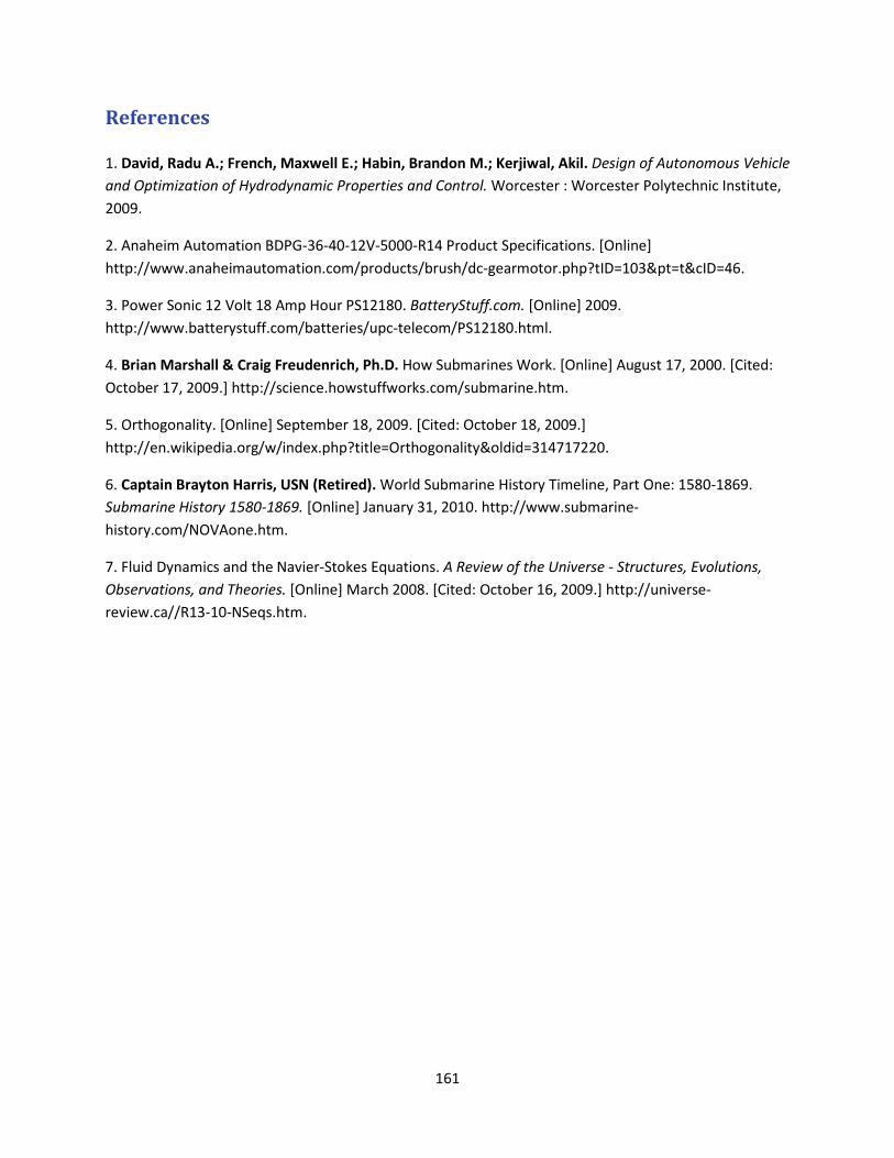
161

References

1. David, Radu A.; French, Maxwell E.; Habin, Brandon M.; Kerjiwal, Akil. Design of Autonomous Vehicle and Optimization of Hydrodynamic Properties and Control. Worcester : Worcester Polytechnic Institute, 2009.

2. Anaheim Automation BDPG-36-40-12V-5000-R14 Product Specifications. [Online] http://www.anaheimautomation.com/products/brush/dc-gearmotor.php?tID=103&pt=t&cID=46.

3. Power Sonic 12 Volt 18 Amp Hour PS12180. BatteryStuff.com. [Online] 2009. http://www.batterystuff.com/batteries/upc-telecom/PS12180.html.

4. Brian Marshall & Craig Freudenrich, Ph.D. How Submarines Work. [Online] August 17, 2000. [Cited: October 17, 2009.] http://science.howstuffworks.com/submarine.htm.

5. Orthogonality. [Online] September 18, 2009. [Cited: October 18, 2009.] http://en.wikipedia.org/w/index.php?title=Orthogonality&oldid=314717220.

6. Captain Brayton Harris, USN (Retired). World Submarine History Timeline, Part One: 1580-1869. Submarine History 1580-1869. [Online] January 31, 2010. http://www.submarine-history.com/NOVAone.htm.

7. Fluid Dynamics and the Navier-Stokes Equations. A Review of the Universe - Structures, Evolutions, Observations, and Theories. [Online] March 2008. [Cited: October 16, 2009.] http://universe-review.ca//R13-10-NSeqs.htm.