Optimising Sweep in the North Sea - OWI APAC 2018:...
36
Optimising Sweep in the North Sea November 5 th 2014, Dr. Branimir Cvetkovic Marsk Oil and Gas AS, Copenhagen-Denmark * Bayerngas Norge AS, Oslo-Norway
Transcript of Optimising Sweep in the North Sea - OWI APAC 2018:...

Optimising Sweep in the North Sea November 5th 2014,
Dr. Branimir Cvetkovic
Marsk Oil and Gas AS, Copenhagen-Denmark
* Bayerngas Norge AS, Oslo-Norway
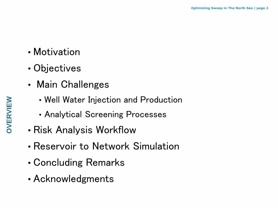
• Motivation
• Objectives
• Main Challenges
• Well Water Injection and Production
• Analytical Screening Processes
• Risk Analysis Workflow
• Reservoir to Network Simulation
• Concluding Remarks
• Acknowledgments
Optimizing Sweep in The North Sea | page 2 O
VE
RV
IEW

CHALLENGES
• North Sea mature fields are declining
• Water injection combined with WAG and SWAG appear to be most dominant recovery processes
• Infill drilling activities together with special water treatment improves recovery
• Other EOR pilot studies are challenging for subsea assets
• Alkaline-Surfactant Polymer flooding remains active
• Downhole Water Separation not Faesible
ACTIVITIES
• Understand the importance of having a good reservoir model with high resolution in order to avoid hazards and analyse any changes within the reservoir
• Assess the technology gaps and breakthroughs that are essential in improving the way that IOR is carried out to ensure improvements in your future projects
• Review the ways in which you can tackle the decline in production from your oil and gas wells through a solid optimisation study
Optimizing Sweep in The North Sea | page 3 M
OT
IVA
TIO
NS
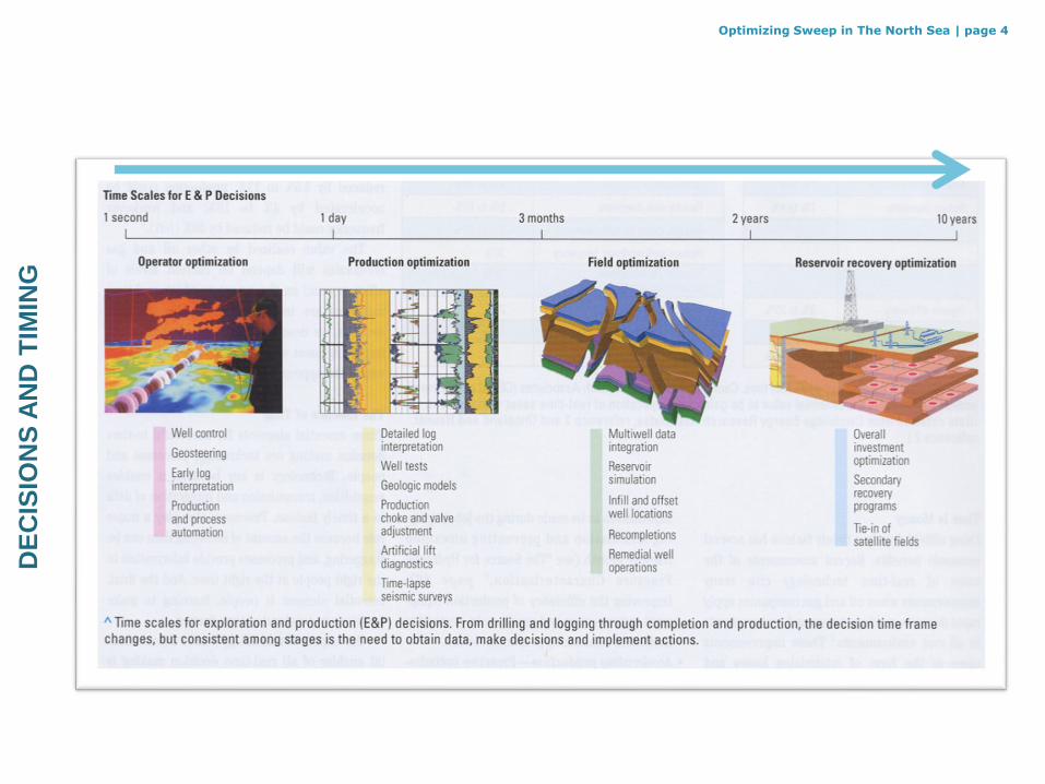
page 4 D
EC
ISIO
NS
AN
D T
IMIN
G
Optimizing Sweep in The North Sea |

Surface Model
Wellbore Model
Well Model
}Reservoir Model
Horizontal
Well
Vertical Well
CO
MP
LE
XIT
Y a
nd
DE
LIV
ER
AB
ILIT
Y
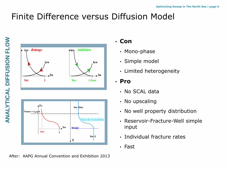
Finite Difference versus Diffusion Model
page 6
• Con
• Mono-phase
• Simple model
• Limited heterogeneity
• Pro
• No SCAL data
• No upscaling
• No well property distribution
• Reservoir-Fracture-Well simple input
• Individual fracture rates
• Fast
After: AAPG Annual Convention and Exhibition 2013
AN
ALY
TIC
AL
DIF
FU
SIO
N F
LO
W
Optimizing Sweep in The North Sea |

Field A - North Sea
• Horizontal well with fractures
• 9 injection wells
• 11 production wells
• Provided data for:
• 2-oil production wells
• 14 fractures
• A water injection well
• 16 fractures
Model V
alid
ation
Nu
meri
cal
vs. A
naly
tic
al – S
cre
en
ing
Meth
od
s
Optimizing Sweep in The North Sea |

Field V - North Sea
0
1
2
3
4
5
6
7
0 100 200 300 400 500 600 700
Time t (Days)
Pro
du
cti
vit
y In
de
x
PI (b
bl/(D
ay
Ps
i)
PI, Productivity index
PI, Productivity index
PI, Productivity index
Fracture Permeability, kf (Fracture width w=0.008 ft)
50 D
15 D
2.5 D
WELL DATA
MFHOW-MODEL DATA
Model V
alid
ation
Pro
ductivity I
ndex P
I [b
bl/(d
Psi)]
Time t (d)
0
1
2
3
4
5
6
7
0 100 200 300 400 500 600 700
Time t (Days)
Pro
du
cti
vit
y In
de
x
PI (b
bl/(D
ay
Ps
i)
PI, Productivity index
PI, Productivity index
PI, Productivity index
Fracture Permeability, kf (Fracture width w=0.008 ft)
50 D
15 D
2.5 D
WELL DATA
MFHOW-MODEL DATA
An
aly
tic
al – P
rod
ucti
on
Scre
en
ing
Meth
od
s
Optimizing Sweep in The North Sea |
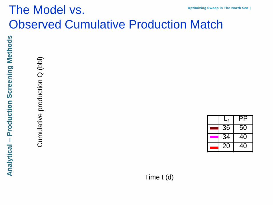
The Model vs.
Observed Cumulative Production Match
Lf PP
36 50
34 40
20 40 Cum
ula
tive p
roduction Q
(bbl)
Time t (d)
Model V
alid
ation
An
aly
tic
al – P
rod
ucti
on
Scre
en
ing
Meth
od
s
Optimizing Sweep in The North Sea |

IBC Changing from
Constant Rate to Constant Pressure SLAB MODEL - RESTART OPTION
Constant Rate to Constant Pressure IBC Changes
0
500
1000
1500
2000
2500
3000
3500
4000
0 100 200 300 400 500 600 700
t (Days)
Pre
ssu
re P
(P
si)
0
1000
2000
3000
4000
5000
6000
7000
8000
Rate
q (
bbl/D
ay)
IBC of Constant:
Rate
Pressure
Variable
Wellbore Rate
Wellbore Pressure
Imple
menta
tion
Time t (d)
Rate
q (
bbl/d)
Pre
ssure
diffe
rence Δ
p (
psi)
An
aly
tic
al – P
rod
ucti
on
Scre
en
ing
Meth
od
s
Optimizing Sweep in The North Sea |

Maching Production History
0.1
1
10
100
1000
10000
100000
0 500 1000 1500 2000 2500 3000 3500
Time, t (Days)
Pre
ss
ure
Dif
ffe
ren
ce
, P
i-P
wf
(ps
i)
0
1
10
100
1000
10000
100000
Model - Variable Pressure Difference, Pi-Pwf Constant Rate, q IBC Well_Pressure_Difference
Conatant Pressure, Pi-Pwf IBC Model - Variable Well with Fractures Rate, q Well_Rates
Back to menu Print Save
Constant Rate, IBC
Constant Pressure, IBC Pressure-difference
varies
for the constant Rate varies for the
constant Pressure-difference IBC
for the constant rate IBC
Time t (d)
Pre
ssure
diffe
rence [
Pi-
Pw
f] (
psi)
Rate
q (
bbl)/d
0.1
1
10
100
1000
10000
100000
0 500 1000 1500 2000 2500 3000 3500
Time, t (Days)
Pre
ss
ure
Dif
ffe
ren
ce
, P
i-P
wf
(ps
i)
0
1
10
100
1000
10000
100000
Model - Variable Pressure Difference, Pi-Pwf Constant Rate, q IBC Well_Pressure_Difference
Conatant Pressure, Pi-Pwf IBC Model - Variable Well with Fractures Rate, q Well_Rates
Back to menu Print Save
Constant Rate, IBC
Constant Pressure, IBC Pressure-difference
varies
for the constant Rate varies for the
constant Pressure-difference IBC
for the constant rate IBC
Model V
alid
ation
An
aly
tic
al – P
rod
ucti
on
Scre
en
ing
Meth
od
s
IBC Changing from Constant Rate to Constant Pressure
Optimizing Sweep in The North Sea |
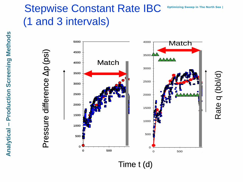
Stepwise Constant Rate IBC
(1 and 3 intervals)
0
500
1000
1500
2000
2500
3000
3500
4000
0 500 1000 1500 2000 2500 3000 3500
Time, t (Days)
Pre
ssu
re D
iffe
ren
ce, P
i-P
wf
(psi
)
0
2000
4000
6000
8000
10000
12000
Wel
lbo
re r
ates
qin
_HO
W (
bb
l/Day
)
P, Pressure difference Press_Diff_Well_Data qin, Input flow rate
Match
Imple
menta
tion
0
500
1000
1500
2000
2500
3000
3500
4000
4500
5000
0 500 1000 1500 2000 2500 3000 3500
Time, t (Days)
Pre
ssu
re D
iffe
ren
ce,
Pi-
Pw
f (P
si)
Pressure Difference (Model) Pressure Difference (Well Data)
Match
Time t (d)
Pre
ssure
diffe
rence Δ
p (psi)
Rate
q (
bbl/d)
0
500
1000
1500
2000
2500
3000
3500
4000
4500
5000
0 500 1000 1500 2000 2500 3000 3500
Time, t (Days)
Pre
ssu
re D
iffe
ren
ce,
Pi-
Pw
f (P
si)
Pressure Difference (Model) Pressure Difference (Well Data)
Match
Time t (d)
Pre
ssure
diffe
rence Δ
p (psi)
An
aly
tic
al – P
rod
ucti
on
Scre
en
ing
Meth
od
s
Optimizing Sweep in The North Sea |

Stepwise Constant
Pressure IBC (3 intervals)
Cumulative production Q (bbl)
Ind
ivid
ua
l F
ractu
re R
ate
q (
bb
l/d
)
Ra
te q
(b
bl/d
)
Infinite Conductivity Fracture
Finite Conductivity Fracture
An
aly
tic
al – P
rod
ucti
on
Scre
en
ing
Meth
od
s
Optimizing Sweep in The North Sea |
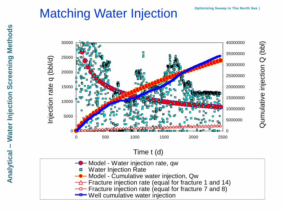
Matching Water Injection
0
5000
10000
15000
20000
25000
30000
0 500 1000 1500 2000 2500
Time, t (Days)
Wa
ter
inje
cti
on
ra
te,
q (
bb
l/D
ay
)
0
5000000
10000000
15000000
20000000
25000000
30000000
35000000
40000000
Cu
mu
lati
ve
wa
ter
inje
cti
on
, Q
(b
bl)
Model - Water injection rate, qwWater Injection Rate Model - Cumulative water injection, QwFracture injection rate (equal for fracture 1 and 14)Fracture injection rate (equal for fracture 7 and 8)Well cumulative water injection
Time t (d)
Inje
ction r
ate
q (
bbl/d)
Qum
ula
tive inje
ction Q
(bbl)
0
5000
10000
15000
20000
25000
30000
0 500 1000 1500 2000 2500
Time, t (Days)
Wa
ter
inje
cti
on
ra
te,
q (
bb
l/D
ay
)
0
5000000
10000000
15000000
20000000
25000000
30000000
35000000
40000000
Cu
mu
lati
ve
wa
ter
inje
cti
on
, Q
(b
bl)
Model - Water injection rate, qwWater Injection Rate Model - Cumulative water injection, QwFracture injection rate (equal for fracture 1 and 14)Fracture injection rate (equal for fracture 7 and 8)Well cumulative water injection
Model V
alid
ation
An
aly
tic
al – W
ate
r In
jecti
on
Scre
en
ing
Meth
od
s
Optimizing Sweep in The North Sea |

Oil Recovery Analytical Injection Rates & Buckley-Leverett
Title of presentation | page 15 A
naly
tic
al – W
ate
r In
jecti
on
Scre
en
ing
Meth
od
s

Reservoir, Well and Fracture Input (Horizontal Well with N Fractures)
• Reservoir
• Isotropic
• Non-isotropic
• Horizontal well
• No flow to the wellbore
• Direct flow to the wellbore
• Wellbore friction
• Model Boundary Conditions
• Inner BC
• Outer BC
Imple
menta
tion
An
aly
tic
al – S
cre
en
ing
Meth
od
s
Optimizing Sweep in The North Sea |

Effective radius and effective half-length
Horizontal
Well
Fracture
Fracture
Vertical Well
Conclu
din
g R
em
ark
s
An
aly
tic
al – W
ell P
rod
ucti
on
Eff
ecti
ve E
sti
mate
s

Late-Time Approximations for Rates
Rate vs. time match for:
• A fractured horizontal well (2 transversal fractures) vs. vertical well with calculated effective radius
• A fractured horizontal well (3- transversal fractures) vs. a single transversal fractured horizontal well with calculated effective half-length
• A fractured horizontal well (3- longitudinal fractures) vs. a single longitudinal fractured horizontal well with calculated effective half-length
0
1000
2000
3000
4000
5000
6000
7000
0 500 1000 1500 2000 2500 3000 3500 4000 4500 5000
Time, t (d)
Rate
, q
(b
bl/d
)
Model data for a horizontal well with two fractures Calculated data for a vertical well with an equivalent well radius
A transient rate calculated data
for the vertical well with a
derived effective well radius
A horizontal well with two
transversal fractures
0
2000
4000
6000
8000
10000
12000
14000
0 500 1000 1500 2000 2500 3000 3500 4000 4500 5000
Time, t (d)
Rate
, q
(b
bl/d
)
Well with the 3 transversal-fractures Well with the single transversal-fracture (with the equivalent fracture half-length)
A transient rate calculated data for the
horizontal well with a derived
equivalent fracture half-length
A horizontal well with three transversal fractures
0
2000
4000
6000
8000
10000
12000
14000
0 500 1000 1500 2000 2500 3000 3500 4000 4500 5000
Time, t (d)
Rate
q (
bb
l/d
)
Well with the 3 longitudinal-fractures Well with the single longitudinal-fracture (with the equivalent fracture half-length)
A transient rate calculated data for the
horizontal well with a derived
equivalent fracture half-length
A horizontal well with three longitudinal fractures
A transient rate calculated data for the
horizontal well with a derived
equivalent fracture half-length
A horizontal well with three longitudinal fractures
Model V
alid
ation
ref
Lef
An
aly
tic
al – W
ell P
rod
ucti
on
Eff
ecti
ve E
sti
mate
s

Exponential
Hyperbolic
Harmonic
q
t
b
Rate-Time Plots M
otivation
• Empirical Arps’ rate-time curves (1945)
• Fetkovich’s composite transient-depletion rate-time curves (1973, 1980)
rD
T
D Mu
lti-
fractu
red
well t
ran
sie
nt
so
luti
on
s
Optimizing Sweep in The North Sea |

Fracture Diagnosis Analyses
• Study is based on the screening analysis of a horizontal well with fractures production data.
• Prognosis profiles were generated manually and compared to the real observed data.
• Study provides workflow for optimising number of fractures along a horizontal well.
• Matching procedure should be further improved with risking tool features for the fracture closure diagnosis.
• The semi-analytical model for a multiple-fractured-horizontal well, was applied providing fast and robust features and were used as screening tools for diagnostic and forecasting purposes.
Conclu
din
g R
em
ark
s
Mu
lti-
fractu
red
well s
olu
tio
ns
Optimizing Sweep in The North Sea |
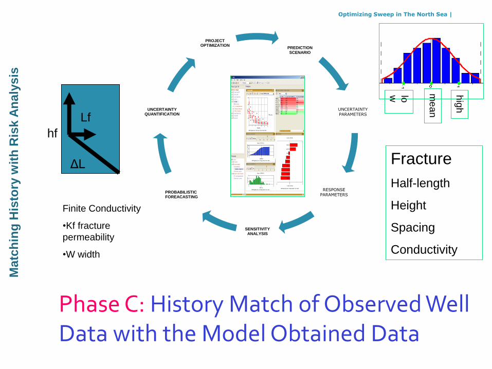
Phase C: History Match of Observed Well Data with the Model Obtained Data
PREDICTION SCENARIO
UNCERTAINTY
PARAMETERS
RESPONSE
PARAMETERS
SENSITIVITY ANALYSIS
PROBABILISTIC FOREACASTING
UNCERTAINTY QUANTIFICATION
PROJECT OPTIMIZATION
hig
h
me
an
low
Fracture
Half-length
Height
Spacing
Conductivity
hf
Lf
ΔL
Finite Conductivity
•Kf fracture
permeability
•W width
Ris
k A
naly
sis
- W
ork
flow
M
atc
hin
g H
isto
ry w
ith
Ris
k A
naly
sis
Optimizing Sweep in The North Sea |
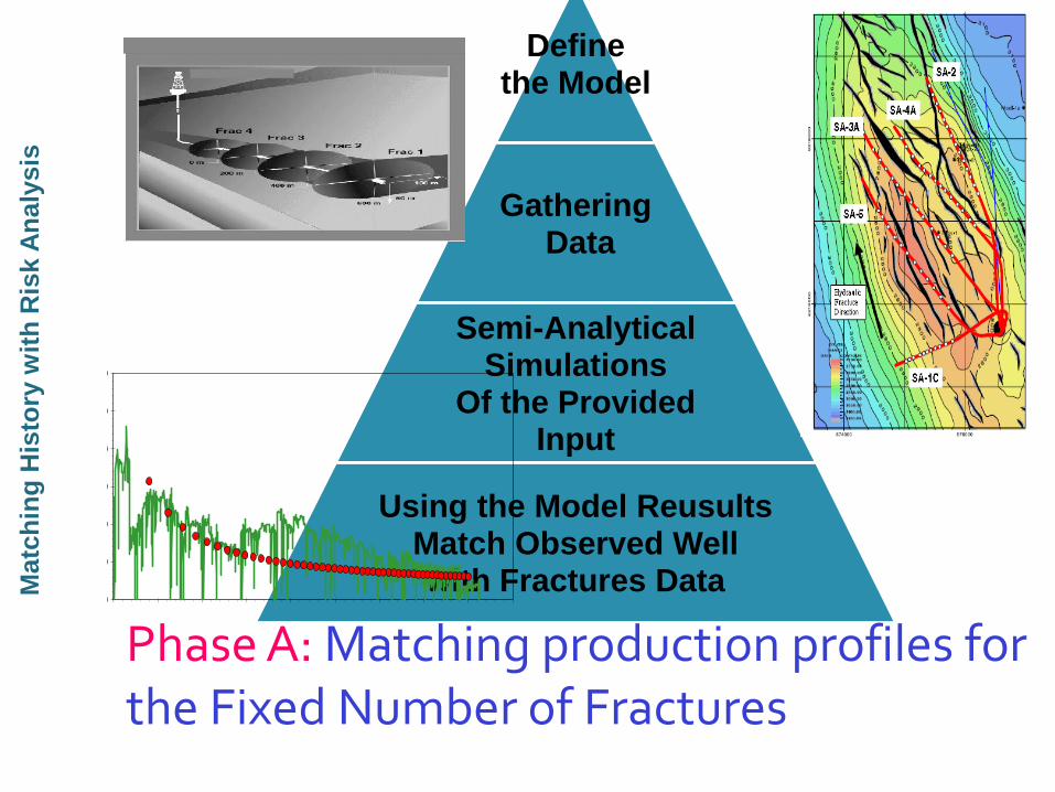
Define the Model
Gathering Data
Semi-Analytical Simulations
Of the Provided Input
Using the Model Reusults Match Observed Well with Fractures Data
0
5000
10000
15000
20000
25000
30000
0 2000000 4000000 6000000 8000000 10000000 12000000 14000000 16000000 18000000
Cumulative rate, Q (bbl)
Rate
, q
(b
bl/
Day
)
Model flow rate, q Well rate, qRis
k A
naly
sis
- W
ork
flow
Phase A: Matching production profiles for the Fixed Number of Fractures
Matc
hin
g H
isto
ry w
ith
Ris
k A
naly
sis

Phase B: Screning Analysis and Optimizing Number of Transversal Fractures Positioned Along a Horizontal Well
PREDICTION SCENARIO
UNCERTAINTY PARAMETERS
RESPONSE PARAMETERS
SENSITIVITY ANALYSIS
PROBABILISTIC FOREACASTING
UNCERTAINTY QUANTIFICATION
PROJECT OPTIMIZATION
•Define ‘Base
Case Model’-
pre-screening
process
hig
h
me
an
low
Reservoir data
Fracture data
Well data
Ris
k A
naly
sis
- W
ork
flow
M
atc
hin
g H
isto
ry w
ith
Ris
k A
naly
sis
2
FRACTURES
hig
h
me
an
low
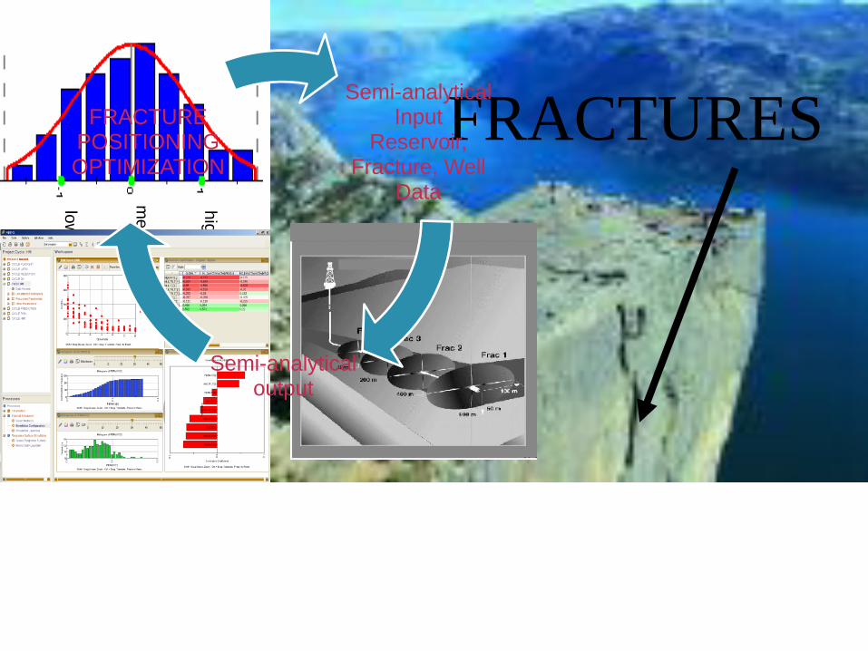
Semi-analytical Input
Reservoir, Fracture, Well
Data
Semi-analytical output
FRACTURE POSITIONING OPTIMIZATION
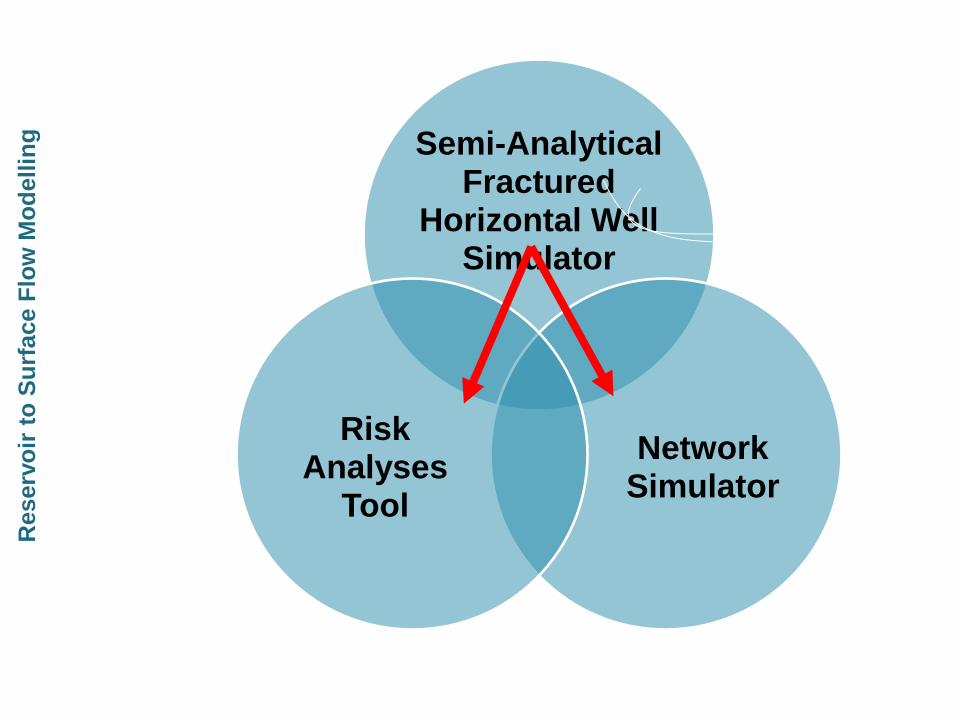
Semi-Analytical Fractured
Horizontal Well Simulator
Network Simulator
Risk Analyses
Tool
Ris
k A
naly
sis
with N
etw
ork
-Reserv
oir
Sim
ula
tion
Reserv
oir
to
Su
rface F
low
Mo
dellin
g

Integral Approach Horozontal Well with Fractures
MATCHING
PROCEDURE
SEMI-
ANALYTICAL
MODEL
- HOWIF
NETWORK
SIMULATOR
METTE
RISK
ANALYSES
MEPO
Ris
k A
naly
sis
with N
etw
ork
-Reserv
oir S
imula
tion
Reserv
oir
to
Su
rface F
low
Mo
dellin
g

Field A North Sea
Fra
ctu
red H
orizonta
l W
ell
with N
etw
ork
Sim
ula
tion
Reserv
oir
to
Su
rface F
low
Mo
dellin
g

Field A with Fractured Horizontal Well
Fra
ctu
red H
orizonta
l W
ell
with N
etw
ork
Sim
ula
tion
Reserv
oir
to
Su
rface F
low
Mo
dellin
g

Horizontal Fractured Wells
Fra
ctu
red H
orizonta
l W
ell
Reserv
oir
to
Su
rface F
low
Mo
dellin
g
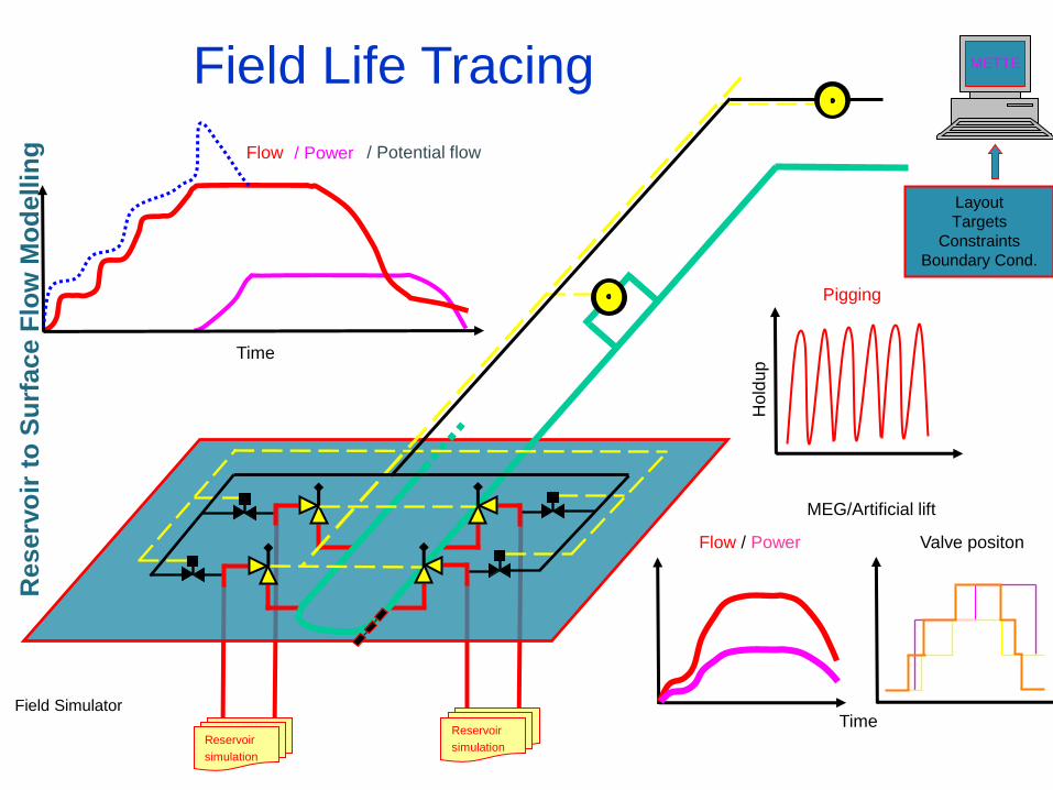
/ Power
Layout
Targets
Constraints
Boundary Cond.
Hold
up
Pigging
000 100 010 001 110 101 011 111 1011 0101
Valve positon
Time
Flow
Time
MEG/Artificial lift
Flow / Power
/ Potential flow
METTE
Field Simulator
Field Life Tracing
Reservoir
simulation
Reservoir
simulation
Motivation
Reserv
oir
to
Su
rface F
low
Mo
dellin
g
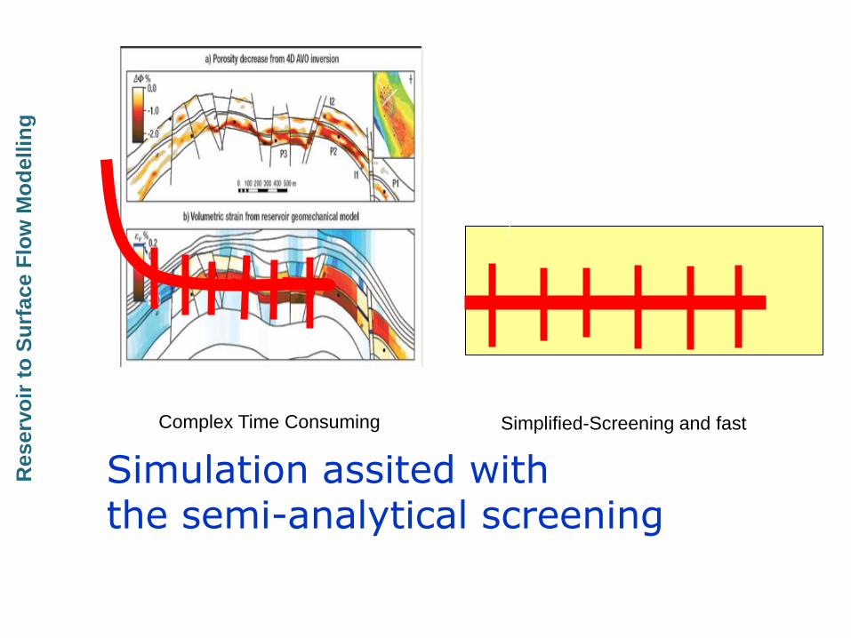
Simulation assited with the semi-analytical screening
Complex Time Consuming Simplified-Screening and fast
Questions
Reserv
oir
to
Su
rface F
low
Mo
dellin
g

• Fast and robust sreening tool for prognostic and diagnosis of fractures along the horizontal well
• Combaining the risk analysis with the network simulation
• Linking the semy-analytical model to the risk analysis software (commercial SW tool as MEPPO Schlumberger)
• Linking the semy-analytical model to a network model (METTE –Yggdrasil A/S, Oslo Norway)
Conclu
din
g R
em
ark
s
SU
MM
AR
Y
• Gudbrand Nerby, Ygddegrita A/S, Oslo Norway
• Ole Jacob Velle, Ygddrasil A/S, Oslo Norway • Asbjørn Sigurdsøn, Yggdrasil A/S, Oslo Norway
• Stefan Djupvik, SPT-Group, Kjeller Norway
• Amerada Hess, Copenhagen
• BP Amoco Stavanger
• Institut for Energy Technololgy IFE Kjeller Norway
Gotskalk Halvorsen, Jan Sagen
• Bayerngas Norge AS, Oslo Norway
Ack
now
ledg
men
ts
AC
KN
OW
LE
DE
NT
S

Questions
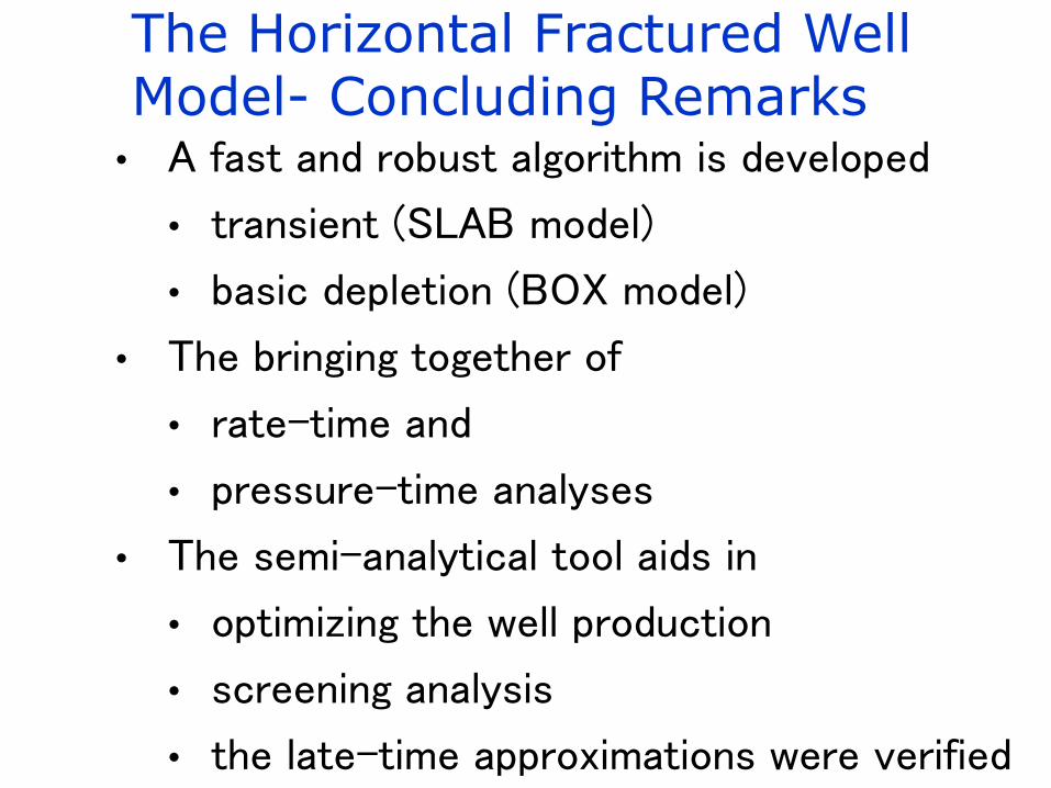
The Horizontal Fractured Well Model- Concluding Remarks
• A fast and robust algorithm is developed
• transient (SLAB model)
• basic depletion (BOX model)
• The bringing together of
• rate-time and
• pressure-time analyses
• The semi-analytical tool aids in
• optimizing the well production
• screening analysis
• the late-time approximations were verified
Model S
um
mary

Fracture Diagnosis Analyses
• Based on screening analysis of a horizontal well with fractures production data.
• Prognosis profiles can be generated and compared to the real observed data.
• Workflow for optimising number of fractures along a horizontal well in prognostic mode.
• Matching procedure combined with the risking tool features improves the fracture closure diagnosis.
• The semi-analytical model for a multiple-fractured-horizontal well, provides fast and robust features and can be used as screening tool for diagnostic and forecasting purposes.
Horizonta
Well
with F
ractu
res P
ossib
le E
xte
nsio
ns