Optimality in Binary Search Trees and Variable-to-Fixed ...Optimality in Binary Search Trees and...

Optimality in Binary Search Trees and

Variable-to-Fixed Length Encoding

by

Mehmet Argun Alparslan

B.Sc., Middle East Technical University, 2005

AN ESSAY SUBMITTED IN PARTIAL FULFILMENT OFTHE REQUIREMENTS FOR THE DEGREE OF

Master of Science

in

The Faculty of Graduate Studies

(Computer Science)

The University Of British Columbia

September, 2007

c© Mehmet Argun Alparslan 2007

Abstract

Binary search tree (BST) is a fundamental data structure widely used foraccesses to ordered data. Despite its wide usage, no online algorithm hasyet been proven to be O(1) competitive to the optimal offline dynamic BSTalgorithm. The first part of this essay surveys different optimality measureswith a greater emphasis on dynamic and static optimality. Lower bounds onthe performance of an optimal dynamic BST are discussed. Online splay treealgorithm which is conjectured to be dynamically optimal and two differentO(lg lg(n)) competitive online algorithms (Tango tree and Multi-Splay tree)are studied.

Secondly variable-to-fixed length scheme of lossless compression is dis-cussed and the entropy lower bound is tied to the static optimality of searchtrees. Different techniques (based on renewal theory and Markov processes)for analyzing plurally parsable dictionaries with memoryless sources andsources with memory are discussed.

ii

Table of Contents

Abstract . . . . . . . . . . . . . . . . . . . . . . . . . . . . . . . . . ii

Table of Contents . . . . . . . . . . . . . . . . . . . . . . . . . . . . iii

List of Figures . . . . . . . . . . . . . . . . . . . . . . . . . . . . . . v

Acknowledgements . . . . . . . . . . . . . . . . . . . . . . . . . . . vi

I Essay 1

1 Static and Dynamic Optimality of Binary Search Trees . . 21.1 Introduction . . . . . . . . . . . . . . . . . . . . . . . . . . . 21.2 Notation & Definitions . . . . . . . . . . . . . . . . . . . . . 31.3 Optimality in Static Binary Search Trees . . . . . . . . . . . 4

1.3.1 Entropy Lower Bound on Static Binary Search Trees 41.4 Splay Trees . . . . . . . . . . . . . . . . . . . . . . . . . . . . 6

1.4.1 Working Set Property . . . . . . . . . . . . . . . . . . 91.4.2 Static Optimality Property . . . . . . . . . . . . . . . 10

1.5 Dynamic Optimality . . . . . . . . . . . . . . . . . . . . . . . 111.5.1 Lower Bounds . . . . . . . . . . . . . . . . . . . . . . 121.5.2 Almost Optimal Data Structures . . . . . . . . . . . . 171.5.3 Other Optimality Measures . . . . . . . . . . . . . . . 25

2 Variable-to-Fixed Length Lossless Data Compression . . 272.1 Introduction . . . . . . . . . . . . . . . . . . . . . . . . . . . 27

2.1.1 Unit of Information . . . . . . . . . . . . . . . . . . . 282.1.2 Variable-to-Fixed Length Encoding . . . . . . . . . . 292.1.3 Plurally Parsable Dictionaries . . . . . . . . . . . . . 352.1.4 Variable-to-Fixed Length Encoding For Sources With

Memory . . . . . . . . . . . . . . . . . . . . . . . . . 43

iii

Table of Contents

3 Conclusion and Future Work . . . . . . . . . . . . . . . . . . 46

Bibliography . . . . . . . . . . . . . . . . . . . . . . . . . . . . . . . 48

iv

List of Figures

1.1 The binary and ternary tree representations. . . . . . . . . . 51.2 Right and Left Rotations . . . . . . . . . . . . . . . . . . . . 71.3 Perfect Tree - 1 . . . . . . . . . . . . . . . . . . . . . . . . . . 131.4 Rectangular Framework Plot . . . . . . . . . . . . . . . . . . 161.5 Auxiliary Trees . . . . . . . . . . . . . . . . . . . . . . . . . . 181.6 Tango Tree - 1 . . . . . . . . . . . . . . . . . . . . . . . . . . 191.7 Perfect Tree - 2 . . . . . . . . . . . . . . . . . . . . . . . . . . 191.8 Tango Split . . . . . . . . . . . . . . . . . . . . . . . . . . . . 211.9 Cut . . . . . . . . . . . . . . . . . . . . . . . . . . . . . . . . 221.10 Tango Tree - 2 . . . . . . . . . . . . . . . . . . . . . . . . . . 221.11 MST - 1 . . . . . . . . . . . . . . . . . . . . . . . . . . . . . . 24

2.1 Prefix Tree - 1 . . . . . . . . . . . . . . . . . . . . . . . . . . 302.2 Prefix Tree - 2 (Unique) . . . . . . . . . . . . . . . . . . . . . 302.3 Markov Chain - 1 (Memoryless) . . . . . . . . . . . . . . . . . 372.4 Markov Chain - 2 (Memory) . . . . . . . . . . . . . . . . . . . 442.5 FSM . . . . . . . . . . . . . . . . . . . . . . . . . . . . . . . . 44

v

Acknowledgements

Foremost I would like to thank my supervisor Will Evans for all his helpand neverending patience from the beginning to the end. I would also liketo thank David Kirkpatrick for reading the essay and sharing his valuablecomments. Finally I would like to thank my family for their solid supportfor the past two years.

vi

Part I

Essay

1

Chapter 1

Static and Dynamic

Optimality of Binary Search

Trees

1.1 Introduction

The binary search tree (BST) is one of the fundamental data structures ex-tensively used for querying membership in sets of ordered data due to itspotential for performing these queries in the time that is logarithmic in thesize of the set. BSTs are widely used for retrieving data from databases,look-up tables and storage dictionaries. Such applications generally needhigh performance when accessing the keys at the nodes. In the past fewdecades there have been various efforts to increase the efficiency of the BSTdata structures by producing new algorithms for balancing the BSTs, al-though none has been proven to be dynamically optimal. In this paperwe will discuss the current optimality measures and new data structuresthat are close to optimal. Moreover we will investigate the variable-to-fixedlength encoding and explore the entropy bounds that tie these two conceptstogether.The first part of the paper will discuss the optimality of BSTs and close-to-optimal BST structures. First we will analyze the optimality criteria for anoffline BST algorithm which is not allowed to update its structure once it isconstructed (i.e. static BST). We will assume that we have prior knowledgeabout the sequence of accesses that will be made to the static BST structureeither by knowing the explicit access sequence or the probability distribu-tion of the access sequence. If not mentioned otherwise we will assume thataccesses in the sequence are independently and identically distributed(i.i.d.).The optimality of the static BSTs is generally known as static optimality.Later we will change our attention to splay trees, a simple online BST algo-rithm, and make a transition to the concept of dynamic optimality. Onlinealgorithms for BST are crucial since the applications that use BSTs gen-

2

Chapter 1. Static and Dynamic Optimality of Binary Search Trees

erally do not know the access sequence in advance. As opposed to staticoptimality no online algorithm has yet been proven to be dynamically opti-mal, so we will elaborate on the dynamic optimality criteria by discussingvarious lower bounds such as Wilber’s first and second lower bound, andDerryberry et al.’s rectangle framework, as well as the data structures suchas Tango trees and Multi Splay trees that were created with these lowerbounds in mind. Finally we will briefly discuss less known optimality mea-sures including dynamic search optimality and key independent optimality.In the second chapter of the paper, we will have a discussion on variable-to-fixed length encoding for channels with fixed capacity. In general finding theoptimal prefix codes for compression can be thought of as constructing theoptimal tree where the probabilities of access for the internal nodes are 0 andthe probabilities of occurrence for the source symbols are known. Thus wewill be linking static optimality to the optimality of variable-to-fixed lengthvia Knuth’s lower bound on static trees. Moreover dynamic trees such assplay trees are also used for adaptive encoding where the codewords rep-resenting the source words change over the time. Our discussion will focuson Tunstall’s algorithm, and plurally parsable codes for memoryless sources.We will discuss two different techniques for analyzing plurally parsable codesfor variable-to-fixed length namely steady-state analysis and renewal theory.Then we will change our direction from memoryless sources to sources withmemory and briefly summarize work that has been done in this area.

1.2 Notation & Definitions

• General Info: Throughout the paper it is assumed that the keys areelements of a totally ordered set Σ. An access sequence A = a1, . . . , am

is a sequence of keys and the node that an access aj visits is denoted asT (aj), where T is the BST. The probability of an access ai is denotedby p(ai) or simply p(i) whereas the frequency of an access is denotedby q(ai) or simply q(i)

• Static BST: A static BST is the one that does not change during theaccess sequence. In other words the static BST is an offline algorithmwhich is presumably aware of the access sequence beforehand.

• Dynamic BST: A dynamic BST is the one that changes during theaccess sequence. We assume that the dynamic BST is an online algo-rithm which does not have prior information about the sequence.

3


1.3 Optimality in Static Binary Search Trees

It is necessary to clearly define the optimality criteria for static BSTs beforewe move onto the algorithms that achieve such optimality. The optimalitycriteria for a static BST can be stated as minimizing the cost of the BSTunder a given access sequence. Such cost can be defined as:

m∑

i=1

d(ai) (1.1)

where d(a) is the depth of the node containing key a. For a sufficiently largesequence of elements (i.e. all the elements in the search tree are touched andthe frequency of accesses is stabilized) we can define the cost of the staticsearch tree with nodes 1, . . . , n:

C =n

∑

i=1

d(i)p(i) (1.2)

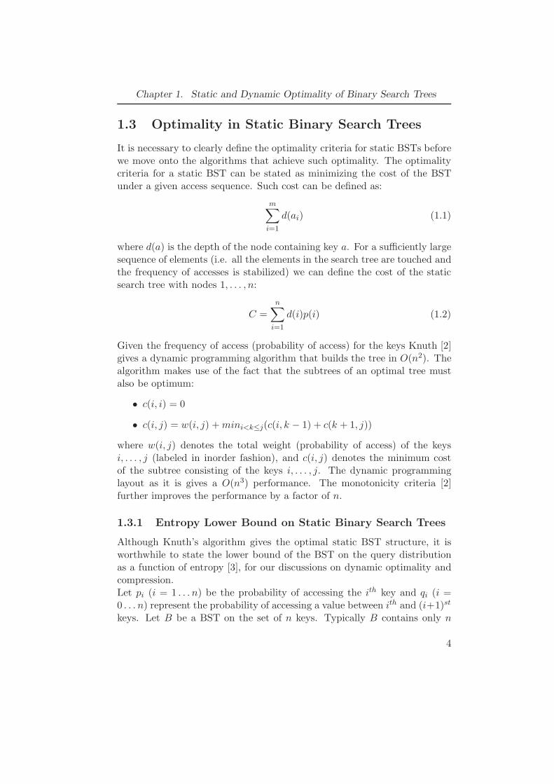
Given the frequency of access (probability of access) for the keys Knuth [2]gives a dynamic programming algorithm that builds the tree in O(n2). Thealgorithm makes use of the fact that the subtrees of an optimal tree mustalso be optimum:

• c(i, i) = 0

• c(i, j) = w(i, j) + mini<k≤j(c(i, k − 1) + c(k + 1, j))

where w(i, j) denotes the total weight (probability of access) of the keysi, . . . , j (labeled in inorder fashion), and c(i, j) denotes the minimum costof the subtree consisting of the keys i, . . . , j. The dynamic programminglayout as it is gives a O(n3) performance. The monotonicity criteria [2]further improves the performance by a factor of n.

1.3.1 Entropy Lower Bound on Static Binary Search Trees

Although Knuth’s algorithm gives the optimal static BST structure, it isworthwhile to state the lower bound of the BST on the query distributionas a function of entropy [3], for our discussions on dynamic optimality andcompression.Let pi (i = 1 . . . n) be the probability of accessing the ith key and qi (i =0 . . . n) represent the probability of accessing a value between ith and (i+1)st

keys. Let B be a BST on the set of n keys. Typically B contains only n

4


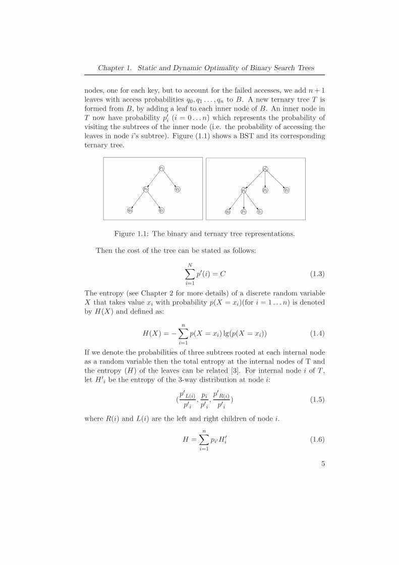
nodes, one for each key, but to account for the failed accesses, we add n + 1leaves with access probabilities q0, q1 . . . , qn to B. A new ternary tree T isformed from B, by adding a leaf to each inner node of B. An inner node inT now have probability p′i (i = 0 . . . n) which represents the probability ofvisiting the subtrees of the inner node (i.e. the probability of accessing theleaves in node i’s subtree). Figure (1.1) shows a BST and its correspondingternary tree.

p1

p0 q2

q0 q1

p′2

p′1

q2

q0 q1

p2

p1

Figure 1.1: The binary and ternary tree representations.

Then the cost of the tree can be stated as follows:

N∑

i=1

p′(i) = C (1.3)

The entropy (see Chapter 2 for more details) of a discrete random variableX that takes value xi with probability p(X = xi)(for i = 1 . . . n) is denotedby H(X) and defined as:

H(X) = −n

∑

i=1

p(X = xi) lg(p(X = xi)) (1.4)

If we denote the probabilities of three subtrees rooted at each internal nodeas a random variable then the total entropy at the internal nodes of T andthe entropy (H) of the leaves can be related [3]. For internal node i of T ,let H ′

i be the entropy of the 3-way distribution at node i:

(p′L(i)

p′i,

pi

p′i,p′R(i)

p′i) (1.5)

where R(i) and L(i) are the left and right children of node i.

H =n

∑

i=1

pi′H′i (1.6)

5


where H ′i is the entropy of the distribution at the internal node i of the tree

T . If the individual normalized probabilities of the three subtrees rootedat internal node i are denoted as r, p, l then the entropy can be bounded asfollows [3]:

H ′(r, p, l) ≤ p lg x + 1 + lg (1 +1

2x) (1.7)

for all x > 0.Using 1.6 and 1.7,

H ≤N

∑

i=1

p′i(pi

p′ilg x + (1 + lg(1 +

1

2x))) (1.8)

≤N

∑

i=1

pi lg x + (1 + lg(1 +1

2x))C (1.9)

If we choose 2x = H/P , where P =∑n

i=1 pi,

H − P lg(H/(2P ))

1 + lg(1 + P/H)≤ C (1.10)

H + P lg e

1 + lg (1 + P/H)− P lg (eH

2P )

1 + lg (1 + P/H)≤ C (1.11)

Since lg(1 + P/H) ≤ (P/H) lg e, we have,

H − P lg (eH

2P) ≤ H + P lg e

1 + lg (1 + P/H)− P lg (eH

2P )

1 + lg (1 + P/H)≤ C (1.12)

Hence the lower bound for the cost of a static binary search tree is Ω(H),where H is the entropy of the probability distribution of the leaves in theternary tree(nodes in the BST B). We are going to use this lower boundwhen proving the static optimality of the splay trees as well as for analyzingthe lower bound of compression for prefix codes as P tends to 0.

1.4 Splay Trees

The data structures that we will be discussing in this section are closelyrelated to splay trees. As well, it is necessary to demonstrate the conceptof optimality on splay trees so that the improvements done via more recentBST data structures can be discussed.

6


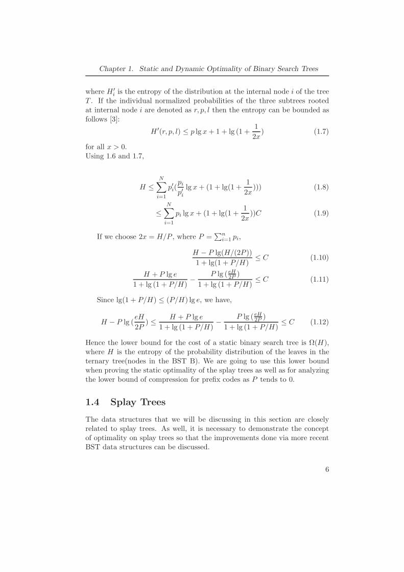
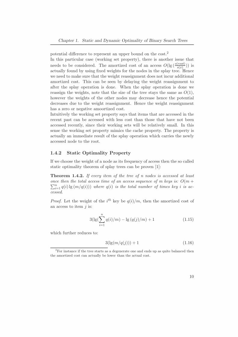
Splay trees [1] are self adjusting binary search trees, which use simple op-erations to keep up with the online processing of the accesses, (and alsopermit insertions and deletions on the set stored by the BST). Unlike otherself balancing trees, splay trees do not use any extra information to manip-ulate the tree. A single splay operation is applied each time an element isaccessed in the tree. Throughout the paper the splay tree (as well as otherbinary search tree data structures) will be considered to be constant in sizealthough the bounds that will be discussed can be applied when insertionsand deletions are permitted.In general, dynamic binary search trees use a combination of 2 differentrotations called left and right (See figure 1.2). Each time an element is ac-

8

4

2 6

4

2 8

6

Right Rotation

Left Rotation

Figure 1.2: Right rotation on 8 (edge 8-4) and left rotation on 4 (edge 4-8).

cessed in a splay tree it is moved (with a number of splay operations) to theroot of the tree. The splay on a node x can be carried out in three differentways using the two generic rotations depending on the relative position ofthe node to its parent and grandparent:

1. zig: If parent(x) is the root of the tree, then a single right/left rotationis carried out, to move x to the root.

2. zigzig: If x and parent(x) are both left or both right children of theirparents, then we perform two zig rotations (edge parent(x)-x and edgex-grandparent(x)).

3. zigzag: If x is a right child of parent(x) and parent(x) is a leftchild of grandparent(x) or vice versa, then we perform one left/rightrotation on x (x-parent(x)) and a right/left rotation on new x (x-grandparent(x)).

Unlike other dynamic BST’s the splay trees do not hold extra informationfor each node and have a relatively simple rotation mechanism. With such

7


simple operations splay trees can achieve competitive bounds for most ac-cesses. However, since splay trees are not forcing any explicit balancingrules some accesses might leave the splay tree completely unbalanced, andcausing the next access to take O(n) time. One example of this is accessingthe nodes in a splay tree in sorted order and then accessing the first itemonce more. Next we will discuss some of the bounds related to splay treeswith an emphasis on a couple of useful properties.First of all it is necessary to bound the cost of a sequence of accesses and thecorresponding splay operations. It is clear that each access operation doesnot have the same effect on the data structure and thus on the potential costof the new shape of the data structure. Because of this reason we wouldneed to do amortized analysis to find the average worst-case performanceof each operation. The potential method of amortized analysis can be usedto calculate the amortized cost of each operation. Informally the potentialmethod keeps track of the potential (prepaid) energy that can be used inthe future. Such potential energy is calculated with respect to the currentstate of data the structure.Let Di denote the state of the data structure after i operations and ci de-note the actual cost of the ith operation. A potential function maps the datastructure Di to a real number Φ(Di), the potential of the data structure.Then the amortized cost c′i of the ith operation is defined as:

c′i = ci + Φ(Di) − Φ(Di−1) (1.13)

where ci is the actual cost of the operation.

n∑

i=1

c′i =n

∑

i=1

ci + Φ(Dn) − Φ(D0) (1.14)

Hence if for all i, Φ(Di) ≥ Φ(D0) then∑n

i c′i is an upper bound on theactual cost of the n operations.The potential method can be applied to the analysis of a splay operation asfollows: Let s(x) be the size of node x where size is defined as the sum ofthe arbitrarily assigned weights of the nodes in the subtree rooted at nodex. Furthermore, define rank r(x) to be lg (s(x)) and the potential of thetree as the sum of the ranks of the nodes in the tree. Intuitively this notionof potential function favors a balanced tree over a degenerate tree, becausea balanced tree would have less potential than an unbalanced (e.g. morelinear) tree thus less potential to have high costs in the future. Sleator andTarjan [1] show the amortized cost of a splay operation at node x is at most

3(r(root) − r(x)) + 1 = O(lg (s(root)s(x) )). The upper bound for the cost of a

8


splay operation does not depend on the choice of the weight for a node. Ingeneral, the weight for a node can be chosen accordingly to prove differentbounds on the splay trees. Next, we will give a couple of the interestingproperties of splay trees proven by choosing different weights that are usedin explanation of the algorithms and bounds in this paper.

1.4.1 Working Set Property

Working set of an access w(j) is defined as the set of distinct keys occurringin the access sequence between ai and aj where ai = aj, and ai is the lastsuch access before aj . The working set property of the splay trees can bestated as follows:

Theorem 1.4.1. The total time spent for an access sequence of length mwith n distinct keys is O(n lg n + m +

∑mi=1 lg(|w(j)| + 1)

Proof. Assign weights 1, 1/4, 1/9, . . . , 1/n2 to the nodes (keys) in their orderof access. When a new access aj occurs only the weight of those key valueswhose weight (1/k2) is larger than weight of aj are updated. The updateresets the weight to 1/(k + 1)2 and weight of aj to 1. Note that this updatekeeps the weights in an ordered sequence from 1 to 1/l2 where l is the numberof distinct keys accessed so far. For example let the access sequence be: x1,x2, x3, x4, x5 then the weights assigned so far are: 1/25, 1/16, 1/9, 1/4,1 . Now if item x2 is accessed next, the weights are reorganized as follows:1/25, 1, 1/16, 1/9, 1/4.Note that with this rearrangement scheme the weight of key aj becomes( 1(|w(j)|+1)2

) just before the access. The amortized cost of access j becomes

O(lg(|w(j)| + 1)) since the size of the root is O(1) (∑n

k=11k2 = O(1)) and

the size of T (aj) is O( 1|w(j)|+1

2). Now the total cost of m accesses becomes

O(∑m

j=1 lg (|w(j)| + 1) + m + n lg n) where O(n lg n) is the maximum initial

potential difference, Φ(D0) − Φ(Dn). 1

Normally in the potential method we could have left the cost as amor-tized cost since it would be a strict upper bound due to monotonicity of thepotential function. However the potential difference Φ(Dn) − Φ(D0) maynot always be positive when we are dealing with splay trees, that is why theamortized cost is not a strict upper bound and we have to add the maximum

1The size of a node can be at most 1, and at least 1/n2, thus the potential differencecan be at most n lg 1

1/n2 =O(n lg n).

9


potential difference to represent an upper bound on the cost.2

In this particular case (working set property), there is another issue that

needs to be considered. The amortized cost of an access O(lg (s(root)s(x) )) is

actually found by using fixed weights for the nodes in the splay tree. Hencewe need to make sure that the weight reassignment does not incur additionalamortized cost. This can be seen by delaying the weight reassignment toafter the splay operation is done. When the splay operation is done wereassign the weights, note that the size of the tree stays the same as O(1),however the weights of the other nodes may decrease hence the potentialdecreases due to the weight reassignment. Hence the weight reassignmenthas a zero or negative amoortized cost.Intuitively the working set property says that items that are accessed in therecent past can be accessed with less cost than those that have not beenaccessed recently, since their working sets will be relatively small. In thissense the working set property mimics the cache property. The property isactually an immediate result of the splay operation which carries the newlyaccessed node to the root.

1.4.2 Static Optimality Property

If we choose the weight of a node as its frequency of access then the so calledstatic optimality theorem of splay trees can be proven [1]:

Theorem 1.4.2. If every item of the tree of n nodes is accessed at leastonce then the total access time of an access sequence of m keys is: O(m +∑n

i=1 q(i) lg (m/q(i))) where q(i) is the total number of times key i is ac-cessed.

Proof. Let the weight of the ith key be q(i)/m, then the amortized cost ofan access to item j is:

3(lg(

n∑

i=1

q(i)/m) − lg (q(j)/m) + 1 (1.15)

which further reduces to:

3(lg(m/q(j))) + 1 (1.16)

2For instance if the tree starts as a degenerate one and ends up as quite balanced thenthe amortized cost can actually be lower than the actual cost.

10


For m access operations this quantity becomes:

3

m∑

i=1

q(i) lg (m/q(i)) + m (1.17)

However this cost is the amortized cost, and Φ(D0)−Φ(Dn) must be addedto find the actual cost of m accesses. The size of node j can be at most∑n

i=1 q(i)/m = 1 and at least q(j)/m, hence the the potential decrease canbe at most:

n∑

j=1

lg (

∑ni=1 q(i)/m

(q(j)/m))) (1.18)

n∑

j=1

lg(m/q(j)) (1.19)

Note that overall actual cost is still O(m +∑n

i=1 q(i) lg(m/q(i))) since thepotential difference is less than the amortized cost since for all i q(i) ≥ 1.So the upper bound is actually O(mH + m) = O(mH) where H is theentropy of the access sequence calculated via the frequency distribution ofthe sequence (i.e. H(A) = −∑n

i=1q(i)m lg q(i)

m ).

This bound achieves the entropy lower bound proved for statically opti-mal binary search trees (See section 1.3.1) [3], hence splay tree is as efficientas an optimal static binary search tree.Not only does this theorem prove that the splay tree data structure per-forms as well as any static BST, but also it shows that the splay tree datastructure does not need to be aware of the frequency of the accessed itemsbeforehand (online algorithm). On the other hand to build a static binarytree with Knuth’s dynamic programming algorithm, one needs to know thecorrect statistics (e.g. frequency) of accessed items.

1.5 Dynamic Optimality

Static optimality deals with the question of whether the data structure pro-cesses accesses on a sequence of i.i.d. items with a performance competitiveto (within a constant factor) a static binary tree optimally constructed forthat sequence. Among many other interesting properties (e.g. working settheorem, static finger theorem, etc.), splay tree data structure is known tobe statically optimal.However a more intriguing question, which has remained unanswered is

11


whether the splay tree or in fact any other tree structure is dynamically op-timal. Dynamic optimality as opposed to static optimality covers a broadersense of optimality by allowing the BST to change over the course of theaccess sequence in the dynamically optimal binary search tree.3 Formallydynamically optimal online algorithm should be c-competitive to the opti-mal offline algorithm, which knows the sequence in advance and performsthe rotations accordingly, splay trees are conjectured to be dynamically op-timal.By the nature of the question it is not possible to directly build a tree andclaim that it is optimal as done in the static optimality. However therehave been found a couple of interesting lower bounds for any BST algorithmacting on a sequence. These bounds may or may not be tight. In the nextsections we will present these lower bounds, then discuss some of the recentdata structures that have been implemented based on these lower bounds.

1.5.1 Lower Bounds

Traditionally the cost of an access to a node at depth d is d plus number ofrotations performed. However this cost can be expressed only in terms ofthe depth of the node (equivalently nodes touched) so that the analysis canbe easier. If we assume that the algorithm first does d rotations to bring thenode to the root, access it and do d reverse rotations to put the node backto its original position then it would run in 2d + 1 time without losing morethan a constant factor of 2. 4 An algorithm that must rotate the accessednode to the root is called a standard search algorithm. Originally Wilber’sfirst bound applied to the standard search algorithm. Iacono’s modifiedlower bound (Interleave Bound) differs from the original bound roughly bya factor of 2 since it does not insist that the accessed element be rotated upto the root.

Wilber’s First Lower Bound Modified (Interleave Bound)

Wilber’s first bound was proposed in 1989 [4], later it was simplified byDemaine et al. [6], and used as the basis for new data structures ([6, 8]).The following version is the one modified by Demaine et al.Let A = a1, a2, . . . , am be an access sequence. Wilber’s first bound gives

3In this paper we will discuss the dynamic trees which change their structures viarotations.

4 We are assuming that the traditional algorithm does not do more than d rotationsto access/re-modify the BST.

12


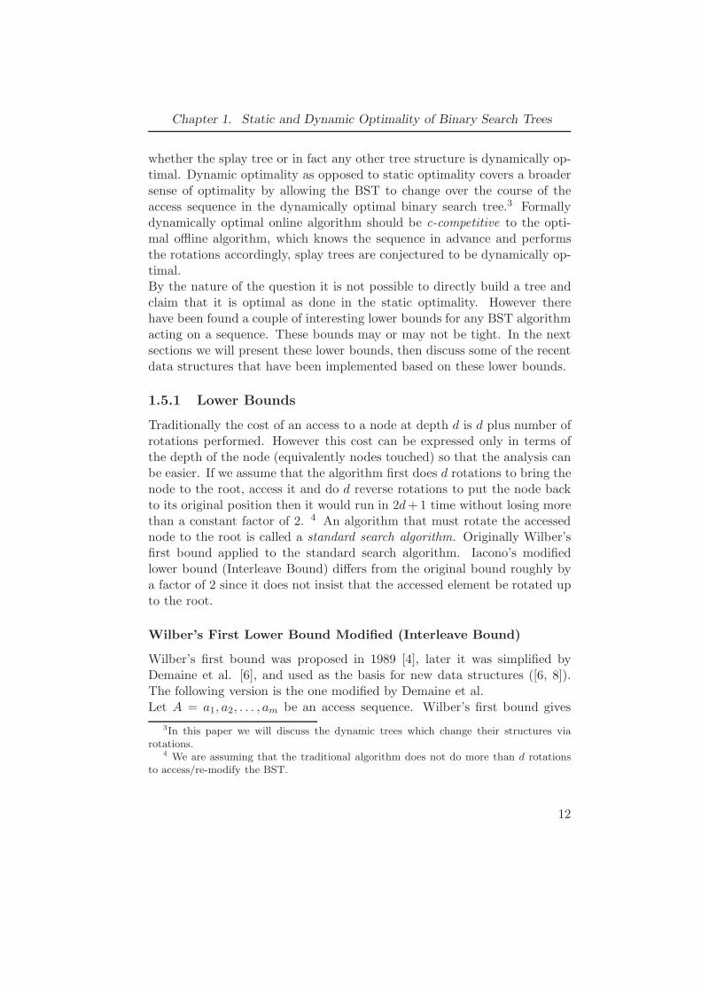
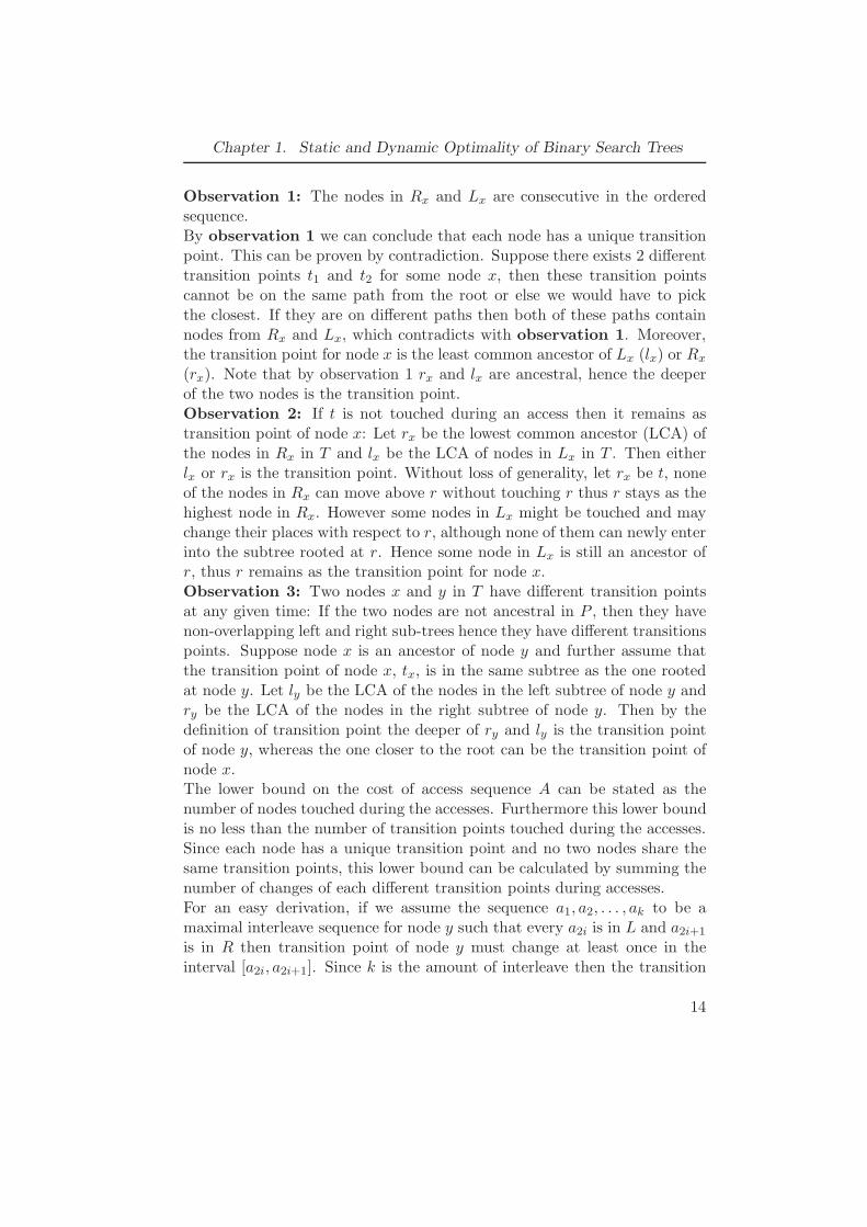
a lower bound on the number of nodes touched in the BST T during theprocessing of the access sequence A. To show the number of such toucheswe will have a second (static) representation of the dynamic BST T . LetP be the perfect binary tree (if n is not 2k for some integer k, then itis a complete binary tree) constructed on the set of n keys of the accesssequence. For each node i, define Li as the left subtree of node i (includingnode i itself) in P and Ri as the right subtree of node i in P . For each accessaj , mark each node in P as R (right) or L (left) depending on which subtreeof the P (aj) resides. (If it does not appear in any subtree, the markingon the node remains unchanged). Figure 1.3 gives a representation on keysΣ = 1, 2, 3, 4, 5, 6, 7, 8, 10, 12, 14, 16, 18, 20, 22, 24, 26, 28, 30, and the accesssequence is 3,22,26,5. Define interleave bound (IB(x)) on node x as the

16 L

8 L

4 R 12

2 R 6 L 10 14

1 3 5 7

24 R

20 R 28 L

18 22 26 30

Figure 1.3: Perfect tree for the keys1, 2, 3, 4, 5, 6, 7, 8, 10, 12, 14, 16, 18, 20, 22, 24, 26, 28, 30, showing the preferred chil-dren and the preferred paths after the access sequence 3,22,26,5.

number of alterations between R and L over the sequence A:

IB(A) =m

∑

i=1

IB(P (ai)) (1.20)

Theorem 1.5.1. The dynamically optimal algorithm performs inΩ(IB(A)/2)

Proof. Let transition point(node) t in tree T of a node x in P to be theclosest node to the root, whose path to root contains at least one node fromRx and one node from Lx.

13


Observation 1: The nodes in Rx and Lx are consecutive in the orderedsequence.By observation 1 we can conclude that each node has a unique transitionpoint. This can be proven by contradiction. Suppose there exists 2 differenttransition points t1 and t2 for some node x, then these transition pointscannot be on the same path from the root or else we would have to pickthe closest. If they are on different paths then both of these paths containnodes from Rx and Lx, which contradicts with observation 1. Moreover,the transition point for node x is the least common ancestor of Lx (lx) or Rx

(rx). Note that by observation 1 rx and lx are ancestral, hence the deeperof the two nodes is the transition point.Observation 2: If t is not touched during an access then it remains astransition point of node x: Let rx be the lowest common ancestor (LCA) ofthe nodes in Rx in T and lx be the LCA of nodes in Lx in T . Then eitherlx or rx is the transition point. Without loss of generality, let rx be t, noneof the nodes in Rx can move above r without touching r thus r stays as thehighest node in Rx. However some nodes in Lx might be touched and maychange their places with respect to r, although none of them can newly enterinto the subtree rooted at r. Hence some node in Lx is still an ancestor ofr, thus r remains as the transition point for node x.Observation 3: Two nodes x and y in T have different transition pointsat any given time: If the two nodes are not ancestral in P , then they havenon-overlapping left and right sub-trees hence they have different transitionspoints. Suppose node x is an ancestor of node y and further assume thatthe transition point of node x, tx, is in the same subtree as the one rootedat node y. Let ly be the LCA of the nodes in the left subtree of node y andry be the LCA of the nodes in the right subtree of node y. Then by thedefinition of transition point the deeper of ry and ly is the transition pointof node y, whereas the one closer to the root can be the transition point ofnode x.The lower bound on the cost of access sequence A can be stated as thenumber of nodes touched during the accesses. Furthermore this lower boundis no less than the number of transition points touched during the accesses.Since each node has a unique transition point and no two nodes share thesame transition points, this lower bound can be calculated by summing thenumber of changes of each different transition points during accesses.For an easy derivation, if we assume the sequence a1, a2, . . . , ak to be amaximal interleave sequence for node y such that every a2i is in L and a2i+1

is in R then transition point of node y must change at least once in theinterval [a2i, a2i+1]. Since k is the amount of interleave then the transition

14


point is changed at least k/2 − 1 times. Summing over all the nodes in thetree this gives the interleave lower bound as IB/2 − n.

Wilber’s Second Lower Bound (Working Set Alternation Bound)

Wilber’s second lower bound [4, 11] connects the cost of an access sequenceto the concept of working sets.Let A = a1, a2, . . . , am be an access sequence, and ai = aj. Assume we insertdistinct ai+1, ai+2, . . . , aj into an initially empty tree in the same order. LetWA(B, j) (working set alternation or Wilber number) denote the number ofalterations between left and right children in the path from the root ai+1 tothe leaf aj . Then

∑

j WA(A, j) gives a lower bound on the access sequenceA. This lower bound is not used in the explanation of the algorithms in thispaper hence we omit the complicated proof of Wilber’s second bound.

Rectangle Framework for Lower Bounds

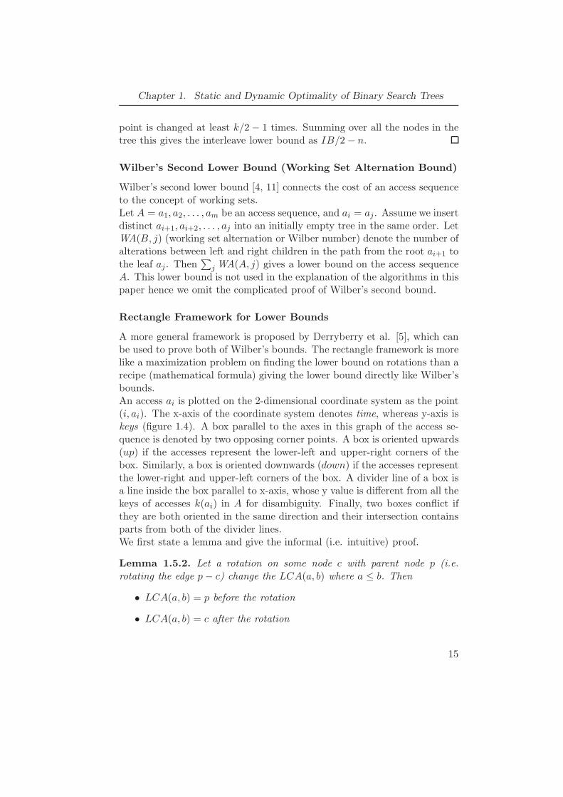
A more general framework is proposed by Derryberry et al. [5], which canbe used to prove both of Wilber’s bounds. The rectangle framework is morelike a maximization problem on finding the lower bound on rotations than arecipe (mathematical formula) giving the lower bound directly like Wilber’sbounds.An access ai is plotted on the 2-dimensional coordinate system as the point(i, ai). The x-axis of the coordinate system denotes time, whereas y-axis iskeys (figure 1.4). A box parallel to the axes in this graph of the access se-quence is denoted by two opposing corner points. A box is oriented upwards(up) if the accesses represent the lower-left and upper-right corners of thebox. Similarly, a box is oriented downwards (down) if the accesses representthe lower-right and upper-left corners of the box. A divider line of a box isa line inside the box parallel to x-axis, whose y value is different from all thekeys of accesses k(ai) in A for disambiguity. Finally, two boxes conflict ifthey are both oriented in the same direction and their intersection containsparts from both of the divider lines.We first state a lemma and give the informal (i.e. intuitive) proof.

Lemma 1.5.2. Let a rotation on some node c with parent node p (i.e.rotating the edge p − c) change the LCA(a, b) where a ≤ b. Then

• LCA(a, b) = p before the rotation

• LCA(a, b) = c after the rotation

15


• a ≤ p ≤ b

• a ≤ c ≤ b

Proof. For the first part we use proof by contradiction. Suppose node p isnot the LCA(a, b) then it can be either above LCA(a, b) in the tree or inone of the subtrees of LCA(a, b). If it is above LCA(a, b) then the subtreecontaining the nodes a and b rotate as one and the LCA(a, b) would stay thesame. Otherwise if node p were on one of the subtrees of LCA(a,b) (w.l.g.suppose one containing a), then this rotation would leave parent of node punmodified thus the LCA(a, b) would stay the same. Immediate from thefirst part node c becomes the new LCA(a, b). Using the results from thefirst two parts of the lemma, and the definition of LCA the third and thefourth results follow.

Figure 1.4: Plotting of an access sequence in time vs keys graph, and example ofnon-conflicting rectangles

Theorem 1.5.3. Let A be an access sequence and B denote the set of pair-wise non-conflicting boxes obtained from the plot of A. Then |B| denotes alower bound on the number of rotations needed to process the access sequenceA.

16


Proof. It is sufficient to show that each such box has at least one uniquerotation, such that no boxes will share the same rotation. The definition(choice) of divider lines become more clear at this rotation assignment. Wedefine a rotation r (p − c rotation) to belong a box (represented by theaccesses ai = a, aj = b), if and only if it is the first rotation that changesthe LCA(a, b) and the line from p to c parallel to y axes crosses the dividerline. Hence a rotation cannot be shared by two different boxes unless theyconflict (i.e. if a rotation is shared by 2 boxes then the rotation line shouldintersect both of the dividers line which means the intersection of the boxescontain part of both of the divider lines). It is also important to note thatthere is at least one such rotation in each box. To see this in figure 1.4 whena is first accessed it is moved to the root hence the LCA(a, b) is a and whenb is accessed the LCA(a, b) becomes b. The LCA of these two nodes changesin between these two accesses thus there is at least one rotation.

The goal of the rectangle framework is finding the maximum number ofpairwise non-conflicting boxes so that the number of these boxes will equalto lower bound on the number of rotations. Finding such a set of non-conflicting boxes is not given by just a recipe, in fact it is claimed that thereis no polynomial time solution for this process. The choice of the boxes andthe placement of the rotation lines determine the lower bound on rotations.Wilber’s lower bounds are proved by these choices.An important open question is whether these lower bounds proposed aretight. In other words are they within a constant factor of the optimal algo-rithm?

1.5.2 Almost Optimal Data Structures

Wilber’s first lower bound inspired researchers to find new data structureswith good optimality bounds. Although up to now no online BST algorithmhas been shown to be dynamically optimal, some are found to be close to theoptimum. Below are two recent BST algorithms based on interleave bound.

Tango Tree

The Tango tree proposed by Demaine et al. [6, 7] performs in O(lg lg n) ofthe interleave bound. The algorithm uses a lower bound tree P as describedin the Wilber’s first bound. A perfect binary search tree is hypotheticallybuilt with the nodes of the actual Tango tree T . For each access, the nodesin P are marked L or R depending on which subtree the most recentlyaccessed node resides on. For each node marked L (respectively R), the

17


preferred child of that node is its left (respectively right) child. A preferredpath is a path, beginning from the root, that follows the sequence of preferredchildren, until it reaches a node with no preferred child.The algorithm from the point of view of perfect lower bound tree P canbe constructed as follows: For access ai the preferred path of this access isextracted following the preferred children. This preferred path is compressedinto an auxiliary tree. Once the first preferred path is removed from Pi, thetree is divided into several pieces of subtrees. Each piece is recursivelyprocessed to find its auxiliary tree, and then these are hung on the originalauxiliary tree. The resulting tree is the tango tree Ti (see figures 1.7,1.5,1.6).

5

4

6

8

16

24

26

28

20

22

12 14

2

3 1 7 18 1030

Figure 1.5: The compressed auxiliary trees (balanced accordingly) constructed byrecursively stripping the preferred paths after the access sequence: 13,22,26,5

After accessing the (i + 1)st element in the sequence, the preferred chil-dren of some of the nodes in Pi will change. Let p be such a parent whosepreferred child switches from L to R. Let L′ be the sub-path (of the old pre-ferred path) that’s rooted at p (i.e. the sub-path below p before the switch),and R′ be the sub-path (of the new preferred path) starting at p and endingat the next switched node. Moreover let U ′ be the sub-path that starts atthe root of P and ends at p. Then the sub-path in the left subtree of p, L′,becomes a preferred path by itself and the sub-path in the right subtree ofp, R′, joins the sub-path leading to p, U ′ . Thus a switch from L to R inthe perfect tree P can be handled by cutting L′ from the original preferredpath and joining U ′ and R′ (See figure 1.7). In the actual implementationof the algorithm the changes in the tango tree are simulated by a single treeT , which consists of multiple auxiliary trees.An auxiliary tree is an augmented red-black tree [12], which stores a pre-

ferred path ordered by the node values. Additionally each node i in the

18


5

4

6

8

16

24

26

28

3020

2218

12

1410

2

31

7

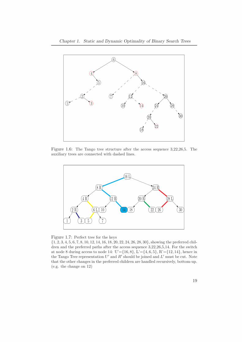
Figure 1.6: The Tango tree structure after the access sequence 3,22,26,5. Theauxiliary trees are connected with dashed lines.

16 L

8 R

4 R 12 R

2 R 6 L 10 14

1 3 5 7

24 R

20 R 28 L

18 22 26 30

Figure 1.7: Perfect tree for the keys1, 2, 3, 4, 5, 6, 7, 8, 10, 12, 14, 16, 18, 20, 22, 24, 26, 28, 30, showing the preferred chil-dren and the preferred paths after the access sequence 3,22,26,5,14. For the switchat node 8 during access to node 14: U’=16, 8, L’=4, 6, 5, R’=12, 14, hence inthe Tango Tree representation U ′ and R′ should be joined and L′ must be cut. Notethat the other changes in the preferred children are handled recursively, bottom-up.(e.g. the change on 12)

19


auxiliary tree holds the node’s actual depth in P (note that P is static),and the depth (in P ) of the deepest node in node i’s subtree. The followingoperations can be carried out efficiently in an augmented red-black tree:

• Splitting an augmented red-black tree at a node x, such that x becomesthe new root of the tree, and both the left and the right subtrees arered-black trees.

• Concatenating two augmented red-black trees whose roots are childrenof the same node x, i.e. re-arranging the subtree of x to form a red-black tree.

Ultimately, using a series of split and concatenate operations the algorithmefficiently performs the following operations on auxiliary trees:

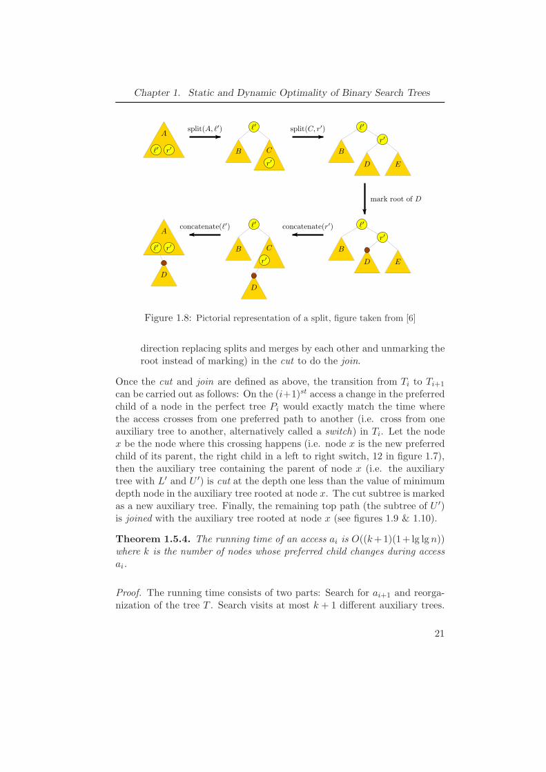
• Cut(d) splits an auxiliary tree for a preferred path π into two trees,one storing the sub-path of π with nodes of depth less than or equal tod and the other storing the sub-path of π with nodes of depth greaterthan d:First an important observation is that nodes in π that have depthsgreater than d form an interval of key space. In other words, no node inπ with depth less than or equal to d can appear between the minimumand the maximum key valued nodes in π with depth greater than d.The observation is trivial yet helps a lot in stripping the nodes withdepth greater than d. With the help of maximum depth informationheld on each node, the key space interval (ℓ′, r′) for depth d can easilybe found. Once the interval is found, splits on both l′ and r′ are carriedout consecutively:split(ℓ′) followed by split(r′)At this point the left subtree of r′, named D, contains the nodes thathave depth greater than d. Next the root of D is marked to denotethat from now on it is an auxiliary tree on its own. The final two stepsare the concatenation of the left out subtrees into one single auxiliarytree (i.e. the tree that contains the path with nodes depth less thand) (see figure 1.8).

• Join two auxiliary subtrees one having the path of nodes with depthless than or equal to d and the other one having the nodes with depthgreater than d. Note that once we find the key space interval of the treewith depth less than d, then we can actually reverse the operations (i.e.start from the end of figure 1.8 and follow the arrows in the opposite

20


A

A

B

r′

r′

r′

r′

C

C

D

D

B

B

D E

B

D E

split(A, ℓ′) split(C, r′)

concatenate(ℓ′) concatenate(r′)

mark root of D

ℓ′ℓ′

r′ℓ′

r′ℓ′

ℓ′ ℓ′

Figure 1.8: Pictorial representation of a split, figure taken from [6]

direction replacing splits and merges by each other and unmarking theroot instead of marking) in the cut to do the join.

Once the cut and join are defined as above, the transition from Ti to Ti+1

can be carried out as follows: On the (i+1)st access a change in the preferredchild of a node in the perfect tree Pi would exactly match the time wherethe access crosses from one preferred path to another (i.e. cross from oneauxiliary tree to another, alternatively called a switch) in Ti. Let the nodex be the node where this crossing happens (i.e. node x is the new preferredchild of its parent, the right child in a left to right switch, 12 in figure 1.7),then the auxiliary tree containing the parent of node x (i.e. the auxiliarytree with L′ and U ′) is cut at the depth one less than the value of minimumdepth node in the auxiliary tree rooted at node x. The cut subtree is markedas a new auxiliary tree. Finally, the remaining top path (the subtree of U ′)is joined with the auxiliary tree rooted at node x (see figures 1.9 & 1.10).

Theorem 1.5.4. The running time of an access ai is O((k +1)(1+ lg lg n))where k is the number of nodes whose preferred child changes during accessai.

Proof. The running time consists of two parts: Search for ai+1 and reorga-nization of the tree T . Search visits at most k + 1 different auxiliary trees.

21


5

4

6

8

16

Split8

4

5 16

6

Concatenate

6

5

8

16

4

Mark

D

8

16

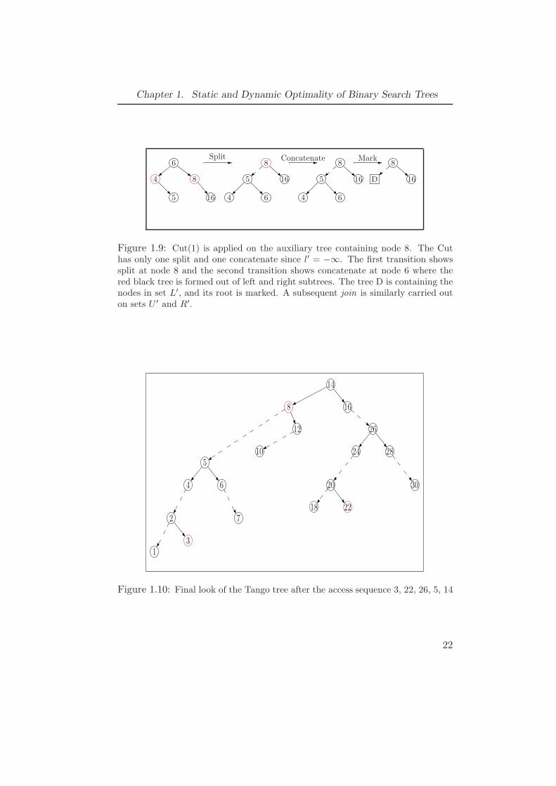
Figure 1.9: Cut(1) is applied on the auxiliary tree containing node 8. The Cuthas only one split and one concatenate since l′ = −∞. The first transition showssplit at node 8 and the second transition shows concatenate at node 6 where thered black tree is formed out of left and right subtrees. The tree D is containing thenodes in set L′, and its root is marked. A subsequent join is similarly carried outon sets U ′ and R′.

14

8 16

12

105

6

7

4

2

13

26

24 28

20

2218

30

Figure 1.10: Final look of the Tango tree after the access sequence 3, 22, 26, 5, 14

22


Since each auxiliary tree can have at most lg n nodes (the length of a pre-ferred path can be at most (lg n), search in one auxiliary tree takes O(lg lg n).Hence the overall search in Tango trees take O((k + 1)(lg lg n + 1)). Updatecost takes O((k+1)(lg lg n+1)) as well since each time the algorithm crossesan auxiliary tree, it performs one cut and one join where both of them take aconstant amount of split and concatenate operations taking O(lg lg n) timein total.

Theorem 1.5.5. The running time of the Tango BST on an input sequenceof m accesses over the universe of n distinct keys is O((OPT (A)+n)(lg lg n+1)).

Proof. The total number of preferred child switches can be at most IB(A)+n(n is added due to initial preferred child settings), combining this with thecost of an access we get O((IB(A) + n + m)(lg lg n + 1)) for the accesssequence A. By the interleave bound the cost of the optimal algorithm isbounded below by IB(A)/2 − n, thus the total time taken by the Tangoalgorithm on sequence A is O((OPT (A) + n)(lg lg n + 1)).

Multi Splay Trees

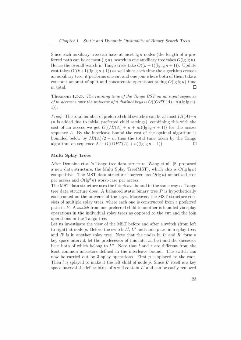
After Demaine et al.’s Tango tree data structure, Wang et al. [8] proposeda new data structure, the Multi Splay Tree(MST), which also is O(lg lg n)competitive. The MST data structure however has O(lg n) amortized costper access and O(lg2 n) worst-case per access.The MST data structure uses the interleave bound in the same way as Tangotree data structure does. A balanced static binary tree P is hypotheticallyconstructed on the universe of the keys. Moreover, the MST structure con-sists of multiple splay trees, where each one is constructed from a preferredpath in P . A switch from one preferred child to another is handled via splayoperations in the individual splay trees as opposed to the cut and the joinoperations in the Tango tree.Let us investigate the view of the MST before and after a switch (from leftto right) at node p. Before the switch L′, U ′ and node p are in a splay tree,and R′ is in another splay tree. Note that the nodes in L′ and R′ form akey space interval, let the predecessor of this interval be l and the successorbe r both of which belong to U ′. Note that l and r are different from theleast common ancestors defined in the interleave bound. The switch cannow be carried out by 3 splay operations. First p is splayed to the root.Then l is splayed to make it the left child of node p. Since L′ itself is a keyspace interval the left subtree of p will contain L′ and can be easily removed

23


14

8 16

12

10

4

2 6

5 71 3

26

24 28

3022

20

18

Figure 1.11: The MST structure after the access sequence 3, 22, 26, 5, 14. Thesplay trees are connected with dashed lines.

from the splay tree (marking the root node). Similarly, splaying on r (tillit becomes right child of node p) brings R′ to its right subtree and can bejoined to the splay tree (by unmarking the root node).If we assume the tree in figure 1.6 is made up of splay trees instead of red-black trees, then node p = 8, and the sets L′, R′ and U ′ remain the sameas in the Tango tree. Now l = 4 is the predecessor of the key space intervalmade up of L′ and R′ and r = 16 is the successor of this interval. Note thatin defining the predecessor we had l ∈ U ′, however this is not possible inthis tree configuration as 4 is the smallest key. Now if we do a zig (left)on 8 (edge 8-16) and another zig (right) on 4 (edge 4-6) we have the con-figuration in figure 1.11. Hence, the left subtree of 8 contains L′ with l = 4as root, and right subtree contains R′ with r = 16 as root. The roots aremarked and unmarked appropriately to complete the switch.

The MST data structure runs in O(OPT (A) lg lg n) time, which is ob-tained in a manner similar to the Tango tree’s competitiveness bound. Thenumber of switches matches the interleave bound and the amortized costper switch can be calculated by taking into account 3 splay operations (each

have O(lg (s(root)s(x) )) amortized cost), and 2 change root operations (each con-

tribute to potential differences in the new tree).

24


On a random access, the MST data structure takes O(lg n) amortized costas opposed to Tango’s O(lg n(lg lg n)) performance, and it can also achievelinear time in sequential accesses.

1.5.3 Other Optimality Measures

The fact that dynamic optimality is still a conjecture for splay trees andno other BST data structure has been found to be dynamically optimal,has lead researchers to define other optimality measures. Below are twooptimality measures that are less restrictive than dynamic optimality andhave been fulfilled by some current BST algorithms.

Dynamic Search Optimality

Cost of an access in a BST can be stated as the cost of rotations and thenumber of nodes touched during the access. Blum et al. [9] proposes a lightercost calculation approach which only takes into account the number of nodestouched during an access (i.e. the depth of the accessed node). In otherwords the rotations come free for the online algorithm. The online algorithmcan rotate freely between two consecutive accesses. The problem is whetherthere exists an optimal online binary search tree algorithm under this costmodel. Blum et al. proposes a simple tree construction algorithm given theprobability distribution of the access sequence. The algorithm reconstructsthe tree for each access, using the updated probability distribution which canbe calculated easily. The reconstruction is free and the cost is calculatedas in the static BST. The cost of this online algorithm is shown to be aconstant multiple of the optimal dynamic offline algorithm, moreover thereconstructed tree at each step has a cost no worse than the entropy ofthe upcoming access sequence. The important result is that the existenceof this algorithm simply negates the possibility of disproving the existenceof dynamic optimality by creating an access sequence and claiming that noalgorithm can process the sequence optimally simply because the search costis too much. Hence, even though dynamic search optimality does not implydynamic optimality, it is a progress against trivially disproving dynamicoptimality for any binary search tree.

Key Independent Optimality

Another interesting optimality is the key independent optimality proposedby Iacono [10]. Let A = a1, a2, . . . , am be the access sequence. Let b be an nto n random bijection from the set of keys Σ to Σ, such that aj is assigned

25


to b(aj). The key independent optimal algorithm processes the sequence Ain O(E[OPT (b(A))]).Normally the performance of an online BST algorithm depends on the fre-quency distribution of the accessed items as well as the proximity of theseaccesses. By taking the expected value among all the possible random bijec-tions the key independent optimality does not take into account the relativedistances between the specific keys, hence is a weaker norm of optimality.By the definition of random bijection, the size of the working set for anaccess i does not change between different bijections. Because of this rea-son any key independent optimal algorithm should process A in O(m +∑m

i=1 lg (w(i) + 1) + m + n lg n), otherwise splay tree algorithm with work-ing set property would perform better. Moreover, using the Wilber’s sec-ond bound, it is shown that the key independent optimal algorithm isΩ(

∑mi=1 lg(w(i))) [10], hence it is Θ(

∑mi=1 lg(w(i))), implying that the splay

tree is a key independent optimal algorithm.

26

Chapter 2

Variable-to-Fixed Length

Lossless Data Compression

2.1 Introduction

Unless any other constraint is desired, lossless compression can be thoughtof as re-representing the information in-hand in such a way that frequentlyused information pieces take less amount of space than infrequently usedones, so that the overall data has a smaller size. The re-represented data iscalled compressed data (alternatively encoding) and the source data is calledsource code or simply source. Converting source to compressed data is calledencoding and converting compressed data into source is called decoding.The application of compression techniques is spread over a broad range ofareas where information is heavily used and stored. Several examples in-clude text compression, audio compression, video/image compression, aswell as naturally occurring ones such as gene compression where frequentlyused genes have fewer nucleotides. Even the words that we use today tendto become smaller as they are more frequently used. The techniques ofcompression differ in various areas and we will focus on lossless compres-sion. A compression scheme is lossless when the decoder can fully recoverthe compressed data into original source. Lossy compression techniques aregenerally used on audio, video/image data where the exact decoding of thecompressed data is not necessary since a human observer is not sharp enoughto sense the differences.In this section we are going to discuss one of the lossless decompressiontechniques, variable-to-fixed length encoding. We will investigate the op-timality of Tunstall’s algorithm, plurally parsable dictionaries for variable-to-fixed length encoding, and variable-to-fixed length encoding for sourceswith memory.

27

Chapter 2. Variable-to-Fixed Length Lossless Data Compression

2.1.1 Unit of Information

To be able to accurately measure the amount of information, we wouldfirst need to choose a unit of measure. Following our frequency analogywe can argue that an event A occurring less frequently would give us moreinformation than an event occurring more frequently. Moreover if we denoteprobability of an event A occurring as p(A), we would get no new informationif p(A) = 1 since we are certain that the event will occur. Thus informationgained from an event increases as the likeliness of the event decreases. Selfinformation of an event A is then defined as − lg(p(A)), which is the numberof bits we need to express the event. For example in a fair coin toss wehave two possible outcomes each having the same probability, thus we canrepresent these two events by a flip of a single bit. Observing heads in thecoin toss would give us 1 bit (nat) of information. Finally, a better way toexpress self information is thinking of it as a measure of surprise in an event.Winning a lottery among a million people would have more surprise thantossing a six in a fair die roll, and in measuring units the first event wouldhave roughly 20 bits of surprise where as the second one would have littleless than 2.5 bits of surprise.Let event A have k possible outcomes as o1, o2, . . . , ok, with probabilities ofobserving the outcomes as p(o1), p(o2), . . . , p(ok). Furthermore, we assumethat each outcome has a distinct numeric value. In other words, we representthe outcomes of event A as a random variable having a certain distribution.Then the expected value of a random variable or an outcome of an event isthe average value of the outcomes of n trials of an event, where n is large:

E[A] =

k∑

i

p(oi)oi (2.1)

We can now define entropy which is the expected information content (sur-prise) of an event with a possible set of outcomes O:

H = −k

∑

i

p(oi) lg(p(oi)) (2.2)

Up to this point we have only set our conventions on information contentand we have not yet related the information content to compression. Letthe source data be comprised of symbols from the set X = x1, x2, . . . , xkwith the occurrence probabilities of p(x1), p(x2), . . . , p(xk), such that eachsymbol is i.i.d., then Shannon’s source coding theorem relates information

28


content and data compression as follows:

(H(X))

lg m≤ E[|c∗(X)|] ≤ H(X)

lg m + 1(2.3)

where c∗ is the optimal (minimum expected length) encoding of X. Weassume that the length of a codeword is the number of symbols in the code-word where the codeword symbols are taken from a set of size m.A more formal explanation of Shannon’s entropy bound (not specifically forsymbol codes) can be done with the concept of asymptotic equipartitionproperty and typical sets.

2.1.2 Variable-to-Fixed Length Encoding

We can view variable-to-fixed length compression in three parts: source,parser and encoder. The (memoryless) source generates i.i.d. symbols. Thesecond part parser takes the source code and generates tokens of varioussizes to be fed into the encoder. Finally, the encoder maps the tokens (sourcewords) partitioned by the parser into codewords. More formally the variable-to-fixed length encoding can be described as a one to one mapping from theset W =w1, w2, . . . , wn to the set C =c1, c2, . . . , cn. Each wi is a variablelength string of symbols from the symbol set X =x1, x2, . . . , xk and eachci is a fixed length string (length=s) of symbols from a symbol set of sizem. Thus the number of different codewords is bounded by ms.The mapping of codewords to source words is stored in a dictionary withM = n entries. The dictionary can be represented as a tree where the leavesrepresent a source word.

Figure 2.1 depicts a tree representation of a dictionary. Each child ofa node is associated with a source symbol. By concatenating the sourcesymbols as we traverse down the tree we obtain a source word representationof a codeword (square nodes). The actual codewords are not shown in thetree since choosing ci or cj for a word wi actually has no importance in termsof compression. The encoder as it reads the source S follows the appropriatebranches of the dictionary tree and generates when it reaches a codewordnode. Once a codeword is generated the encoder restarts from the root of thetree 5. By this algorithm we can conclude that a dictionary tree is complete(i.e. can encode every possible source sequences) only if every path fromthe root contains a codeword node. A tree is called a prefix tree when nosource word is a proper prefix of another, similarly it is called a non-prefix

5Note that some short sequences of source symbols may not have codewords but thereare only a finite number of these

29


b c

aa ab ac

p(a)p(b)

p(c)

p(a)p(b)

p(c)

Figure 2.1: A prefix dictionary tree for aa, ab, ac, b, c

a b c

aaaa

p(a)

p(a)

p(a)

p(a)

p(b)p(c)

Figure 2.2: A plurally parsable dictionary tree for aaaa, a, b, c

30


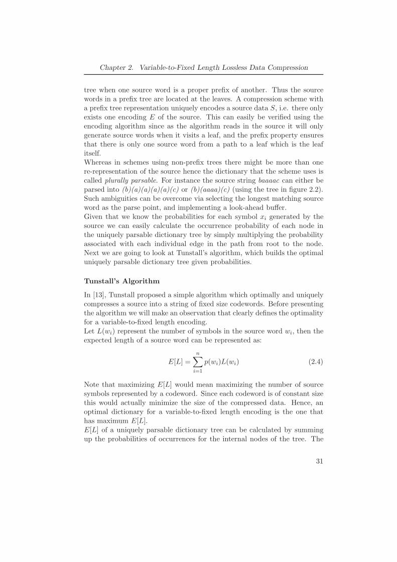
tree when one source word is a proper prefix of another. Thus the sourcewords in a prefix tree are located at the leaves. A compression scheme witha prefix tree representation uniquely encodes a source data S, i.e. there onlyexists one encoding E of the source. This can easily be verified using theencoding algorithm since as the algorithm reads in the source it will onlygenerate source words when it visits a leaf, and the prefix property ensuresthat there is only one source word from a path to a leaf which is the leafitself.Whereas in schemes using non-prefix trees there might be more than onere-representation of the source hence the dictionary that the scheme uses iscalled plurally parsable. For instance the source string baaaac can either beparsed into (b)(a)(a)(a)(a)(c) or (b)(aaaa)(c) (using the tree in figure 2.2).Such ambiguities can be overcome via selecting the longest matching sourceword as the parse point, and implementing a look-ahead buffer.Given that we know the probabilities for each symbol xi generated by thesource we can easily calculate the occurrence probability of each node inthe uniquely parsable dictionary tree by simply multiplying the probabilityassociated with each individual edge in the path from root to the node.Next we are going to look at Tunstall’s algorithm, which builds the optimaluniquely parsable dictionary tree given probabilities.

Tunstall’s Algorithm

In [13], Tunstall proposed a simple algorithm which optimally and uniquelycompresses a source into a string of fixed size codewords. Before presentingthe algorithm we will make an observation that clearly defines the optimalityfor a variable-to-fixed length encoding.Let L(wi) represent the number of symbols in the source word wi, then theexpected length of a source word can be represented as:

E[L] =n

∑

i=1

p(wi)L(wi) (2.4)

Note that maximizing E[L] would mean maximizing the number of sourcesymbols represented by a codeword. Since each codeword is of constant sizethis would actually minimize the size of the compressed data. Hence, anoptimal dictionary for a variable-to-fixed length encoding is the one thathas maximum E[L].E[L] of a uniquely parsable dictionary tree can be calculated by summingup the probabilities of occurrences for the internal nodes of the tree. The

31


E[L] of a prefix tree with only root as an internal node and k leaves is 1. Ifwe assume that hypothesis holds for I − 1 internal nodes and the codewordwith maximum probability to be cI−1 then the EI [L] of a prefix tree with Iinternal nodes can be expressed as:

EI [L] = EI−1[L] − d(cI−1)p(cI−1) +

k∑

i=1

p(xi)p(cI−1)(d(cI−1) + 1) (2.5)

EI [L] = EI−1[L] +

k∑

i=1

p(xi)p(cI−1) (2.6)

EI [L] = EI−1[L] + p(cI−1) (2.7)

Now that we have a natural way of calculating E[L], we can denote thealgorithm that maximizes E[L] as follows:Let x1, x2, . . . , xk be the characters of the source. Start with a single node,root with the associated probability 1. Repeatedly choose the leaf withhighest probability and add k children to it where ith child has associatedprobability p(xi) times the probability of its parent. Stop when the nextaddition would result in a tree with more than M leaves where M is thedictionary size.To show that Tunstall’s algorithm finds the optimal set of dictionary withsize M (i.e. maximizes the E[L]) we take a full k-ary tree with depthI = M

k−1 − 1, whose inner node probabilities are calculated as in Tunstall’salgorithm. Note that any uniquely parsable dictionary tree with I innernodes, is a subtree of this k-ary tree. The maximum expected length E[L]can be achieved by picking the I greatest inner node probabilities. Let thisset be D = q1, q2, ...qI where the inner nodes qi are ordered with respectto their probabilities, and q1 is the root node having the probability 1. Notethat this set is actually connected (i.e. forms a tree): Let qi be a node inD, i 6= 1 then p(qp) > p(qi), thus qp should also be in the ordered set D.Now it suffices to show that at ith step, Tunstall’s algorithm picks qi as aninner node. This can be proven by induction: At step 1, Tunstall’s algorithmpicks the root as inner node which is same as q1. Assume that Tunstall’salgorithm picks q1, . . . , qt until step t ≥ 2. At step t+1 since the nodes in Dare connected, qt+1 should be a child of one of q1, . . . , qt, moreover qt+1 mustbe the greatest probability child whose probability is less than or equal toqt, due to the choice of the set D. Note that Tunstall’s algorithm will selectthe maximum probability child as qt+1.Although we have proved that Tunstall’s algorithm is an optimal algorithm

32


we can still show that the algorithm reaches the entropy bound as the num-ber of dictionary entries tend to infinity. Using (2.3) we can denote theentropy bound as follows:

(H(X))

lg m≤ s

E[L](2.8)

where the right hand side becomes expected codeword length per sourcesymbol. Before proving the following:

(H(X)) = limM→∞s lg m

E[L](2.9)

We first need following two lemmas [17]:

Lemma 2.1.1. Let H(X) denote entropy of the probability distribution ofthe source symbols and H(C) denote the entropy of the compressed output.Then:

H(C) = H(X)E[L] (2.10)

Proof. We will prove this lemma by induction: If there is a single sourcesymbol then H(S)=H(C)=0. Let HI(C) denote the entropy of the com-pressed data whose dictionary tree has I internal nodes. Let c∗I+1 represent

the last internal node extracted during Tunstall’s algorithm for (I + 1)st

internal node. Then we can define HI+1(S) as follows:

HI+1(C) = −∑

ci∈(C−c∗I+1)

p(ci) lg(p(ci)) −∑

xi∈X

p(xi)p(c∗I+1) lg(p(xi)p(c∗I+1))

= HI(C) + p(c∗I+1) lg(p(c∗I+1)) − p(c∗I+1)(−H(X) + lg(p(c∗I+1)))

= EI(L)H(X) + p(c∗I+1) lg(p(c∗I+1))

+p(c∗I+1)H(X) − p(c∗I+1) lg(p(c∗I+1))

= H(X)(EI(L) + p(c∗I+1))

= H(X)EI+1(L)

Lemma 2.1.2. Let max(C) denote maxc∈C(p(c)) and similarly min(C)denote minc∈C(p(c)), then the following inequality holds:

max(C)

min(C)≤ min(X)(−1) (2.11)

33


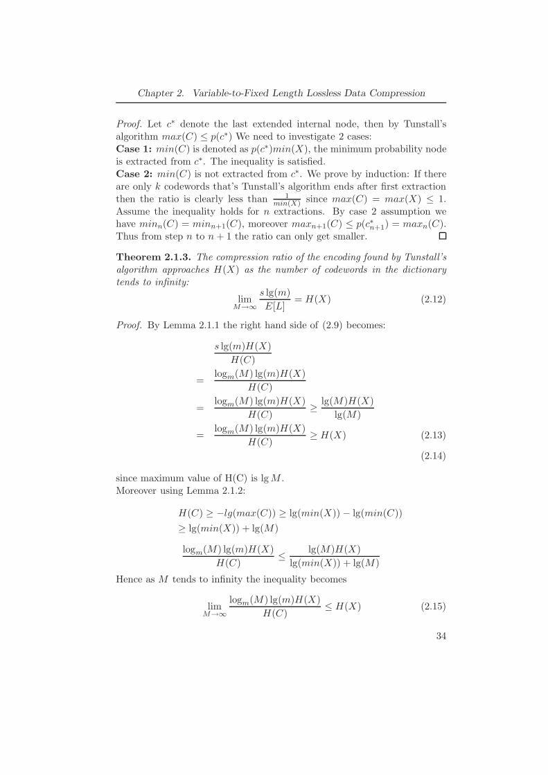
Proof. Let c∗ denote the last extended internal node, then by Tunstall’salgorithm max(C) ≤ p(c∗) We need to investigate 2 cases:Case 1: min(C) is denoted as p(c∗)min(X), the minimum probability nodeis extracted from c∗. The inequality is satisfied.Case 2: min(C) is not extracted from c∗. We prove by induction: If thereare only k codewords that’s Tunstall’s algorithm ends after first extractionthen the ratio is clearly less than 1

min(X) since max(C) = max(X) ≤ 1.Assume the inequality holds for n extractions. By case 2 assumption wehave minn(C) = minn+1(C), moreover maxn+1(C) ≤ p(c∗n+1) = maxn(C).Thus from step n to n + 1 the ratio can only get smaller.

Theorem 2.1.3. The compression ratio of the encoding found by Tunstall’salgorithm approaches H(X) as the number of codewords in the dictionarytends to infinity:

limM→∞

s lg(m)

E[L]= H(X) (2.12)

Proof. By Lemma 2.1.1 the right hand side of (2.9) becomes:

s lg(m)H(X)

H(C)

=logm(M) lg(m)H(X)

H(C)

=logm(M) lg(m)H(X)

H(C)≥ lg(M)H(X)

lg(M)

=logm(M) lg(m)H(X)

H(C)≥ H(X) (2.13)

(2.14)

since maximum value of H(C) is lg M .Moreover using Lemma 2.1.2:

H(C) ≥ −lg(max(C)) ≥ lg(min(X)) − lg(min(C))

≥ lg(min(X)) + lg(M)

logm(M) lg(m)H(X)

H(C)≤ lg(M)H(X)

lg(min(X)) + lg(M)

Hence as M tends to infinity the inequality becomes

limM→∞

logm(M) lg(m)H(X)

H(C)≤ H(X) (2.15)

34


since lg(min(X)) is constant.The proof is completed by equations 2.13 & 2.15 , the squeeze theorem.

If we were to present the dictionary codewords used in the Tunstall’salgorithm as the leaves of a m-ary tree, then we can reach the entropybound by using Knuth’s entropy bound for the optimal static BSTs. Firstthing to point out is that although we proved the bound for BST’s thereis no reason we cannot use the same bound for the m-ary trees. Havingconstructed the m-ary tree we see that the probabilities pi for the internalnodes are actually 0, since the m-ary tree is a prefix tree. We see thatKnuth’s bound (1.8) tends to H as P tends to 0.

2.1.3 Plurally Parsable Dictionaries

Tunstall’s algorithm gives the optimal encoding for uniquely parsable dic-tionaries. However, when the dictionary is not uniquely parsable, that is, ina path from the root to a leaf, there is more than one codeword, we need todo some more analysis to find the optimal dictionary. In this section, twodifferent methods that are used to analyze the optimality of a dictionarywill be discussed [18]. These methods rely on the concepts of Markov chainsand renewal theory.

Discrete Time Markov Chains

A stochastic process is a collection of random variables S(t) (denoted by St)where t is often taken as time, and the random variable S(t) is called thestate that the process is in at time t. The first order discrete time Markovchain is a stochastic process where time takes discrete values and the statevariable obeys the following Markov criteria:

p(St = j|S0 = s0, S1 = s1 . . . St−1 = i) = p(St = j|St−1 = i) = Tij (2.16)

which is sometimes articulated as the future depends only on the present(not the past). Tij is called the state transition probability from state i tostate j where T is an N × N matrix.

N∑

j=0

Tij = 1 (2.17)

Furthermore T nij denotes the probability of reaching state j from state i in

n time steps.

35


State j is said to be accessible from state i, if there exists some n < ∞ suchthat T n

ij > 0. State i is said to communicate with state j, if the two statesare accessible to each other. Maximal set of states communicating eachother is called a class, and if the Markov chain has only one class then it iscalled irreducible. State i is said to be transient if the process will re-enterthe state with probability less than 1 (in other words the system has somesink states), conversely state i is said to be recurrent if with probability 1the process will re-enter state i, and positive recurrent if the amount of timethe process to re-enter is finite. Finally, state i is said to have a period dif T n

ij = 0 whenever n is not divisible by d and is the largest such integer.Therefore, if state i can be visited at time steps 4, 8, 12, . . . then the periodis 4 but not 2 as 4 is the largest integer that satisfies the periodicity. It canbe shown that all the properties such as recurrence, transiency, periodicityare class properties as well (e.g. if a state in a class is recurrent then all thestates in the class are recurrent).Now that we have set forth the definitions for Markov chains we can state animportant result on Markov chains that we will make use of in the analysis.Let T n denote the state transition probability matrix after n time steps. Leta denote the initial state probabilities of the Markov process, then an, stateprobabilities after n steps, is defined as follows:

an = (T )na (2.18)

If the Markov process is irreducible ergodic (positive recurrent and aperi-odic) then the state probability an converges as number of time steps tendsto infinity. If we take π as follows:

π = limn→∞

an (2.19)

then it is necessary to have the following inequality since π converges:

π = Tπ (2.20)

Solution of (2.20) gives the steady state probability vector (π). Finally, thesteady state probability vector is also equivalent to the amount of (normal-ized) time that the process spends in each state. 6

Steady State Analysis for Optimal Plurally Parsable Dictionaries

Assume that the source alphabet is comprised of 2 symbols X=0, 1 andthe probabilities of occurrence for these 2 symbols be p(0) >> p(1)), (i.e.

6Intuitively after the series converges to π the amount of time that the process spendsin state i will also converge to πi in a sufficiently long time.

36


symbol ’0’ occurs much more frequently than symbol ’1’). For a dictionary ofsize limited to 3, Tunstall’s algorithm creates the following optimal uniquelyparsable dictionary W =00, 01, 1 with E[L] = 1 + p(0). However, sincethe probability of occurrence for the symbol ’1’ is very low, it is obviousthat ’01’ will not be used as frequently as ’00’ or a long run of 0’s. Hence,if we do not confine the solution to the uniquely parsable dictionaries it ispossible to get better compression for the same size limit. Let W ′ =0, 1, 0lbe the plurally parsable dictionary then E[L′] of W ′ can be calculated usingthe steady state analysis:A discrete time Markov process with states:S =S0, S1, S00, S000, . . . , S0l−1 , S0l1is formed. States S0i denotes the parsing point where the scanned output isthe same as the states, whereas states S0,S00, . . . , S0i=l−1 denote the parsingpoints where there are i 0’s before the next 1. Note that the Markov processis complete in the sense that the process is in some state for every possibleinput sequence (even though it might have to look-ahead for most of thesequences). Finally, state transitions are carried out according to the sourceoutput. An example Markov chain for l = 3 is shown in figure 2.3. Thestates S0 and S00 are ”dummy” states that are used so that the sum ofthe stationary probabilities (times one) is the expected length of the sourceword. A small discussion on the correctness of the Markov chain for l = 3

S0 S1

S00 S000 000

1

∅

01

001000∅

011

001

S0 S1

S00 S000 000

1

1

p0p1

p02p1

p031

p0p1

p1

p02p1

Figure 2.3: State transition diagram and the corresponding Markov chain for theplurally parsable dictionary of 0, 1, 000

is needed before we move on to steady state analysis. The Markov chainformed with the mentioned recipe is aperiodic: both states S1 and S0l haveself transitions hence it is possible to remain in those states at every time

37


step. Moreover, states S0i<l have empty transitions to S0i−1 which can befollowed all the way to state S1 or S0l which in turn have one step transitionsback to S0i<l . Hence, we can find the steady state probabilities for Π1 = π1,Π0 =

∑l−1i=1 Πi

0, Π0l = π0l which also gives the proportion of time that theMarkov chain is in those states. Note that the empty transitions on Si

0 letsthe ’0’s in the source output to be iteratively parsed. For example if wehave ’001’ for l = 3, then the Markov chain will be in states S0, S00, S1 atthe same time so that the steady state probability will add up p1p0

2 threetimes, to correctly set the expected length.The steady state analysis of the Markov chain yields the following probabilitydistributions:

Π0l =p1

1/p0l − 1 − p1(l − 1)

(2.21)

Π0 =(1/p0)

l−1 − 1 − p1(l − 1)

(1/p0)l − 1 − p1(l − 1)(2.22)

Π1 =p1((1/p0)

l − 1)

1/p0l − 1 − p1(l − 1)

(2.23)

E[L] = Π0 + Π1 + lΠ0l (2.24)

E[L] =((1/p0)

l − 1)

1/p0l − 1 − p1(l − 1)

(2.25)

It can be verified that the expected length for plurally parsable dictionarygets larger than that of uniquely parsable by correctly setting the value ofl with respect to p0. However a more interesting result that verifies ourintuition is that as the probability of p0 approaches 1 the expected lengthof the plurally parsable dictionary grows unboundedly as opposed to thatof uniquely parsable dictionary with the constant size (1 + p0), because asp0 tends nearer to 1 we start to see longer and longer sequences of ’0’s andthe expected number of symbols (mostly 0’s) covered by a single dictionaryentry gets bigger and bigger. To show this, we take derivative with respectto l and find the value of l that maximizes E[L], the maximizing l valuebecomes [18]:

E[L∗] =

√

1

2 ln(1/p0)+ 1/12 +

o(√

1/p0)√

ln(1/p0)(2.26)

As the expected length of source string covered by a codeword increasesunboundedly, the compression ratio reaches to the entropy bound. To seethis, we set s lg(m) to 2 in (2.8) which is the number of bits needed to

38


represent one codeword. Since we have 3 entries in the plurally parsabledictionary we would need 2 bits per codeword. Now the compression ratiobecomes:

2√

12 ln(1/p0) + 1/12 +

o(√

1/p0)√ln(1/p0)

(2.27)

which shows that the compression ratio converges fast to H(X) = 0 as p0

approaches 1. Hence, plurally parsable dictionaries can achieve the entropybound with limited size dictionaries as long as p0 is chosen close enough to1.As the number of symbols in the source alphabet grows the steady stateanalysis would require more work, since the number of states increase lin-early. In the next section, we will discuss an alternative analysis techniquebased on renewal theory which is easier to carry out for a subset of sourcedistributions.

Basics on Renewal Theory

A counting process [15] N(t), t ≥ 0 is a stochastic process where N(t)denotes the number of events occurring before or on time t. The countingprocess satisfies the following properties:

• N(t) ≥ 0

• N(t) is integer valued.

• If s < t then N(s) ≤ N(t)

• For s < t N(t) − N(s) is the number of events that occur in (s, t]

Let Xi denote the time that passes between the (i−1)st and the ith events (in-ter arrival/wait time), then the counting process is called a renewal processif the sequence X1,X2, . . . ,Xn, is independently and identically distributed.Let Si denote the time of the ith event:

Sn =

n∑

i=1

Xi (2.28)

then the expected wait time for an event is derived by:

E[X] = limn→∞

∑ni=1 Xi

n= µ (2.29)

Note that Si denoting the time of the ith event and the Si denoting the stateof the Markov process are two different entities and it will be clear from thecontext that which one we are using.

39


Renewal Theory Analysis of Plurally Parsable Dictionaries

For sources where the occurrence probability of one symbol is much higherthan the rest of the symbols (very predictable sources) there is actually aneasier way to analyze the plurally parsable dictionary for the variable-to-fixed length encoding [18]. For the source from the previous example wecan create dictionaries whose source words do not have symbol ’1’ or havesymbol ’1’ only at the end of the entry. For example the dictionary from thelast section 1, 0, 0l is valid whereas D =1, 0, 0l/210l/2 is not. We wouldexpect the ’1’s in the source words to appear at the end as they have verylittle probability. Thus the points where symbol ’1’ occur are guaranteed tobe end of a source word and can be taken as a regeneration point of a newevent. An event is defined to be an occurrence of symbol ’1’ in the output,thus an event represents an integral amount of source words in the output.Let time be denoted by the number of source words occurring in the sourceoutput and let N(t) denote the number of 1’s that have appeared in thefirst t source words. It can be easily shown that the process N(t), t ≥0 is a counting process as it satisfies the four properties of a countingprocess, moreover it is a renewal process since the occurrence place of a ’1’is independently and identically distributed from the previous occurrence ofthe symbol. Moreover:

• Xi denotes the number of symbols (not the number of source words)emitted between the (i − 1)st and ith occurrence of 1, including the(i − 1)st.

• Si denotes the place of the ith occurrence of the symbol 1

• Lk denotes the length of the kth parsed source word

Note that in this setting time t is measured in two different ways. Timet appearing in N(t) is expressed as number of source words whereas timethat Xi denotes is expressed in terms of number of symbols. However bothof these representations are equivalent and can be converted to each other.Then by the definition of N(t) and Sn we have the following inequality:

SN(k) ≤k

∑

i=1

Li < SN(k)+1 (2.30)

If for example, the first 10 source words included only 3 ’1’s (N(10) = 3)then the place of the 3rd ’1’ is before or equal to the last character of the10th source word depending on whether the 10th source word ends with a

40


’1’. If the source word does not end with a ’1’ then the last character of thesource word occurs after the 3rd occurrence of symbol 1. The last characterof the 10th source word clearly occurs before the 4th ’1’.By (2.28):

limk→∞

∑N(k)i=1 Xi

N(k)

N(k)

k≤

∑ki=1 Li

k<

∑N(k)+1i=1 Xi

N(k)

N(k)

k(2.31)

By strong law of large numbers we have:

E[L] = limk→∞

∑ki=1 Li

k(2.32)

1

p1= lim

k→∞

∑N(k)i=1 Xi

N(k)(2.33)

1

E[S]= lim

k→∞

N(k)

k(2.34)

where E[S] denotes the expected number of parsed source words betweentwo consecutive occurrences of the symbol ’1’. Now we have:

(E[S]p1)−1 ≤ E[L] ≤ (E[S]p1)

−1 (2.35)

The result obtained in (2.35) is intuitive since E[S] is number of source wordsbetween each 1, and E[S]p1 is the number of source words per character.Thus the reciprocal will give the number of characters per source word. Theanalysis of the dictionary from the previous section is given below:

E[S] =

∞∑

j=0

p0jp1w(0j1) (2.36)

where w(S) is the number of source words parsed in the string S. For thedictionary 0, 1, 0l (when longest matched dictionary entry is selected):

w(0j1) =

j+1 if j < lj-l+2 if l ≤ j ≤ 2l

j-2l+3 if 2l ≤ j ≤ 3l...

41


Hence we have:

E[S] = p1 + 2p1p0 + 3p1p02 + · · · + lp1p0

l−1

+2p1pl0 + 3p1p

l+10 + 4p1p0

l+2 + · · · + (l + 1)p1p02l−1

+3p1p2l0 + 4p1p

2l+10 + 5p1p0

2l+2 + · · · + (l + 2)p1p03l−1

...

LetA = 1 + 2p0 + 3p0

2 + 4p03 + · · · + lp0

l−1 (2.37)

B = 1 + p0 + p02 + · · · + p0

l−1 (2.38)

Then

E[S] = p1A + p1p0l(A + B) + p1p0

2l(A + 2B) + . . . (2.39)

E[S] = p1A(1 + p0l + p0

2l + . . . ) + p1p0lB(1 + 2p0

l + 3p02l + . . . ) (2.40)

E[S] = p1A1

1 − p0l+ p1p0

lB1

(1 − p0l)

2 (2.41)

Note that:

A =d(

∑li=0 p0

i)

dp0=

1 − pl+10

(1 − p0)2 − (l + 1)p0

l

1 − p0(2.42)

B =1 − p0

l

1 − p0(2.43)

E[S] =1 − p0

l + p1p0l(1 − l)

p1(1 − p0l)

(2.44)

E[L] =

(

1 − p0l + p1p0

l(1 − l)

(1 − p0l)

)−1

(2.45)

Even though it is easier to analyze the behavior of the plurally parsable dic-tionaries, the approach is limited to the sources that are highly predictable.Savari in her paper [18] discusses the uses renewal theory for finding theoptimal dictionaries with size M + 2, M ≥ 2 where the source output prob-ability satisfies p0 ≥ p1. The renewal theory approach can be generalized tosource alphabets with k ≥ 2 such that E[L] = ((1 − p0)E[R])−1 where p0 isthe most probable symbol.

42


2.1.4 Variable-to-Fixed Length Encoding For Sources With

Memory

So far we have focused on the sources where each symbol generated bythe source is independent from the symbols that are emitted before. Suchsources are called memoryless in the sense that the source does not needto know what it has generated in the previous rounds. However there aremany real life sources that act on the contrary. For instance, if the character’h’ in the English language has an individual occurrence probability of p(h),then p(h|t), the probability of occurrence for the character ’h’ given the lastcharacter read from the source was ’t’, would be much higher due to thehigh frequency of the word ’the’. Hence for such sources we would need toconsider the conditional probability of occurrence for a symbol dependingon the previous symbol(s) emitted, to get lower entropy results.Such a source is also called a Markov source since it can be represented asa discrete Markov process, where the probability of emitting each symboldepends on the state that the process is in. Let Xk denote the kth symbol,then

P (Xk = x|Sk−1 = s,Xk−1 = xk−1 . . . S1 = s1,X1 = x1) (2.46)

= P (Xk = x|Sk−1 = s) (2.47)

= Q(x|s) (2.48)

F (Xk, Sk) = Sk+1 (2.49)∑

xs.t.F (X,Si)=Sj

Q(x|Si) = Tij (2.50)

Here F (x, Si) is the next state transition function. We assume that the pre-vious state and the output symbol determine the next state.We will discuss two different approaches for close-to-optimal solutions [20,21] based on creating different dictionaries for each state of the Markov pro-cess. Let the source alphabet be 0, 1, and the distribution for the symbolsbe as follows: p(0) = 0.5, p(1) = 0.5, p(0|0) = .9, p(1|1) = .9, so the sourceemits long sequences of 1’s and 0’s and avoids the alternating sequences.The Markov process for the source is shown in figure 2.4 where the statesS0 and S1 denote the last emitted symbol.There is another intermediate finite machine (other than the Markov chainof the source) that we need to present in order to sketch the analysis for de-riving E[L]. This finite machine has the same states with the source Markov

43


chain. These states are called parsing points. The parsing points representthe last character of the source word parsed, and acts as a point to checkthe dictionary for the next source word to be parsed. In other words thestate transitions are made by parsing a dictionary word as opposed to read-ing a character from the source. Figure 2.5 represents the finite machine ofthe dictionary 0, 10, 11 with the appropriate states (parsing points) andthe transitions among them according to the dictionary entries. The steadystate probabilities of the finite machine are denoted by ρ(0) and ρ(1), whichrepresent the normalized amount of time each state is chosen as a pars-ing point for the new source word. Now the analysis of E[L] should takeinto account which state the source Markov chain is in because the statesdetermine the probability of occurrence for each character. Moreover, theanalysis should also take into account the steady state probability distribu-tion of the parsing points since this distribution determines the amount oftime spent on each parsing point.

S0 S10/.9 1/.9

1/.1

0/.1

Figure 2.4: Markov chain for the source with memory

S0 S110, 0 11

11

10, 0

Figure 2.5: Finite state machine of the dictionary 0, 10, 11

The probability of occurrence for the source words can be listed as:

P (0) = p(0|0)ρ(0) + p(0|1)ρ(1) (2.51)

P (01) = p(01|0)ρ(0) + p(01|1)ρ(1) (2.52)

44


P (11) = p(11|0)ρ(0) + p(11|1)ρ(1) (2.53)

ρ(0) = P (0) + P (10) (2.54)

ρ(1) = 1 − ρ(0) (2.55)

Note that in 2.51 if p(0|0) = p(0|1) (i.e. memoryless source) then we wouldnot need ρ(0), ρ(1). Now the expected length of a source word becomes:

E[L] = P (0) + 2P (10) + 2P (11) =19

14(2.56)

Since the probability of occurrence for each symbol varies as the state ofthe Markov process changes, it is plausible to construct a different dictionaryfor each state. This idea was first introduced by Tjalkens and Willems [20]for a slightly different source word construction than that of Tunstall’s. Thealgorithm chooses a step size for each character xi and state Sj , which islogarithmically proportional to the Q(xi|sj). Then a prefix tree is built forevery state such that the total step size of a source word ’sx’ in the treeis greater than a constant K (analogous to the dictionary size M of theTunstall’s algorithm), and total step size of ’s’ is less than K. For sourcewords defined in this way the algorithm’s compression ratio converges theentropy of the symbols for sufficiently large K. Using the step size of thesource words, a total ordering among the source words can be established, sothat the index of the source word and the step size can be uniquely mappedto each other. Thus the algorithm does not need to do a table look-up tomatch the source words to codewords.Later Savari and Gallager [21], using Tunstall’s way of constructing theprefix tree, proposed a new analysis technique based on the renewal theory,and devised a way to create an ǫ-optimal set of dictionaries (policy) thatis independent of the parsing point probabilities. The algorithm greedilyconstructs optimal dictionaries (of size M) for each state with Tunstall’salgorithm, and it does not take into account the steady state probabilitiesof the Markov chain which depends on the dictionary entries. The analysisshows that the dictionary (union of individually created dictionaries for eachstate) differs from the entropy bound by Θ((ln M)−1), and policy p is ǫ-optimal such that the expected length E[Lp] is at most as worse as anyother policy by a factor of ǫ, where E[Lp] is defined as:

N∑

i=1

E[LSi ]ρi (2.57)

45

Chapter 3

Conclusion and Future Work

In this paper, we have investigated certain optimality measures related tobinary search trees and variable-to-fixed length compression and gave spe-cific examples where necessary. The optimality of the BSTs is consideredin two main categories as static and dynamic optimality. Static optimal-ity, dealing with constructing the optimal static BST, have been resolveda long time ago by Knuth’s O(n2) dynamic programming algorithm. Laterthe online splay tree algorithm was shown to be statically optimal, whichdrew attention to the dynamic trees and dynamic optimality. At first thestatically optimal online splay tree algorithm was conjectured to be dynam-ically optimal. However, no new information resolving the conjecture hasbeen found since then and the researchers started to direct their studies to-ward finding close to optimal algorithms (e.g. Tango Trees and Multi SplayTrees), mainly using Wilber’s first lower bound for trees with rotations.These two fundamentally similar algorithms are O(lg lg(n)) competitive todynamically optimal offline BST. As the dynamic optimality still remainsan open question, the researchers are finding different optimality measuressuch as the key independent optimality and the dynamic search optimalityto help proving dynamic optimality. An important part of the research haverelied on the Wilber’s first bound and it is possible that new data struc-tures can be found using different lower bounds. The rectangle framework,which is more general than the both of Wilber’s bounds is a good candidate,however there are still questions about the tightness of the bound found bythe framework. Other possible research areas occur from the computationalcomplexity of the rectangle framework algorithm which is very likely to benon-polynomial.The second part of our paper investigated the tree based lossless compressionscheme, variable-to-fixed length encoding. The cost function of compressionand the cost function for BSTs are two very similar concepts, hence weshowed that the lower bound for static BSTs (Knuth’s entropy bound) canbe induced to the bound of compression in the limiting case where innernode probabilities of the tree tends to 0. Tunstall’s algorithm finds theoptimal uniquely parsable dictionary for memoryless sources, however the

46

Chapter 3. Conclusion and Future Work

results can be improved for plurally parsable dictionaries. We discussed twodifferent approaches to analyze plurally parsable dictionaries and derivedthe optimal dictionary for a certain form. Finally, we discussed the morerealistic scenario where the source emitting probabilities follow that of aMarkov process. With more probability information gained in this way, itis certain that the entropy of the source will decrease and the compressionratio will increase. It is also noted that a greedy algorithm which constructsthe dictionaries for each state of the Markov source, performs competitiveto the entropy bound of the source.

47

Bibliography

[1] Sleator, D. D & Tarjan, R.E. Self Adjusting Binary Search Trees ACM,1985.

[2] Knuth D. E. The Art of Computer Programming-Vol-2 p:433-439, Ad-dison Wesley Pub, 1973.

[3] Knuth D. E. The Art of Computer Programming-Vol-2 p:443-445, Ad-dison Wesley Pub, 1991.

[4] Wilber, R. Lower Bounds For Accessing Binary Search Trees With Ro-tations SIAM, 1989.

[5] Derryberry, J., Sleator D. D., Wang, C.C. A Lower Bound Frameworkfor Binary Search Trees with Rotations ACM-SIAM Symposium on Dis-crete Algorithms, 2005.

[6] Demaine, E.D., Harmon D., Iacono J., Patrascu M. Dynamic Optimal-ity Almost Foundations of Computer Science, IEEE, 2004.

[7] Demaine, E.D., Harmon D., Iacono J., Patrascu M. Dynamic Optimal-ity Almost SIAM, 2007.

[8] Wang, C.C., Derryberry, J., Sleator D. D. O(lg lg(n))-Competitive Dy-namic Search Trees ACM-SIAM Symposium on Discrete Algorithms,2006.

[9] Blum, A., Chawla, S., Kalai, A. Static Optimality and Dynamic Search-Optimality in Lists and Trees ACM-SIAM Symposium on Discrete Al-gorithms, 2002.

[10] Iacono, J. Key Independent Optimality International Symposium onAlgorithms and Computation, 2002.

[11] Demaine, E. Lecture Notes:4 , Advanced Data Structures Course, MIT,Spring 2005.

48

Bibliography

[12] Cormen T.H., Leiserson C.E., Rivest R.L, Stein C. Introduction ToAlgorithms p:270-317, McGraw Hill, 2002.

[13] Tunstall B.P., ”Synthesis of Noiseless Compression Codes”, Ph.D. Dis-sertation, Georgia Inst. Tech., Atlanta, GA, Sept., 1967.

[14] Ross, Sheldon M. Introduction to Probability Models p:181-248, Aca-demic Press, 2003.

[15] Ross, Sheldon M. Introduction to Probability Models Chpt:7, AcademicPress, 2003

[16] Heyman, Daniel P., Sobel Mathew J. Stochastic Models In OperationsResearch Vol 1, Sec. 9.1, Dover Publications, 1982.

[17] Jelinek, F., Schneider K. S. On Variable-Length-to-Block Coding IEEETransactions on Information Theory, Vol. IT-18, No.6 November, 1972.

[18] Savari, Serap A. Renewal Theory and Source Coding Proceedings of theIEEE, Vol. 8, No.11, November , 2000.

[19] Gallager, Robert G. Notes on Information Theory: Variable-to-FixedLength Source Coding, 1992.

[20] Tjalkens, Tjalling J., Willems, Frans M. J. Variable-to-Fixed-LengthCodes for Markov Sources IEEE Transactions on Information Theory,Vol. IT-18, No.6 November, 1987.

[21] Savari, Serap A., Gallager, Robert G. Generalized Tunstall Codes forSources With Memory IEEE Transactions on Information Theory, Vol.43, No.2 March, 1997.

49

Optimality in Binary Search Trees and Variable-to-Fixed ...Optimality in Binary Search Trees and...

Documents

Transcript of Optimality in Binary Search Trees and Variable-to-Fixed ...Optimality in Binary Search Trees and...