Optimal Tuner Selection for Kalman Filter-Based … · Donald L. Simon and Sanjay Garg Glenn...

Donald L. Simon and Sanjay GargGlenn Research Center, Cleveland, Ohio

Optimal Tuner Selection for Kalman Filter-BasedAircraft Engine Performance Estimation

NASA/TM—2010-216076

January 2010

GT2009–59684

https://ntrs.nasa.gov/search.jsp?R=20100006914 2018-08-14T15:24:38+00:00Z

NASA STI Program . . . in Profi le

Since its founding, NASA has been dedicated to the advancement of aeronautics and space science. The NASA Scientifi c and Technical Information (STI) program plays a key part in helping NASA maintain this important role.

The NASA STI Program operates under the auspices of the Agency Chief Information Offi cer. It collects, organizes, provides for archiving, and disseminates NASA’s STI. The NASA STI program provides access to the NASA Aeronautics and Space Database and its public interface, the NASA Technical Reports Server, thus providing one of the largest collections of aeronautical and space science STI in the world. Results are published in both non-NASA channels and by NASA in the NASA STI Report Series, which includes the following report types: • TECHNICAL PUBLICATION. Reports of

completed research or a major signifi cant phase of research that present the results of NASA programs and include extensive data or theoretical analysis. Includes compilations of signifi cant scientifi c and technical data and information deemed to be of continuing reference value. NASA counterpart of peer-reviewed formal professional papers but has less stringent limitations on manuscript length and extent of graphic presentations.

• TECHNICAL MEMORANDUM. Scientifi c

and technical fi ndings that are preliminary or of specialized interest, e.g., quick release reports, working papers, and bibliographies that contain minimal annotation. Does not contain extensive analysis.

• CONTRACTOR REPORT. Scientifi c and

technical fi ndings by NASA-sponsored contractors and grantees.

• CONFERENCE PUBLICATION. Collected papers from scientifi c and technical conferences, symposia, seminars, or other meetings sponsored or cosponsored by NASA.

• SPECIAL PUBLICATION. Scientifi c,

technical, or historical information from NASA programs, projects, and missions, often concerned with subjects having substantial public interest.

• TECHNICAL TRANSLATION. English-

language translations of foreign scientifi c and technical material pertinent to NASA’s mission.

Specialized services also include creating custom thesauri, building customized databases, organizing and publishing research results.

For more information about the NASA STI program, see the following:

• Access the NASA STI program home page at http://www.sti.nasa.gov

• E-mail your question via the Internet to help@

sti.nasa.gov • Fax your question to the NASA STI Help Desk

at 443–757–5803 • Telephone the NASA STI Help Desk at 443–757–5802 • Write to:

NASA Center for AeroSpace Information (CASI) 7115 Standard Drive Hanover, MD 21076–1320

Donald L. Simon and Sanjay GargGlenn Research Center, Cleveland, Ohio

Optimal Tuner Selection for Kalman Filter-BasedAircraft Engine Performance Estimation

NASA/TM—2010-216076

January 2010

GT2009–59684

National Aeronautics andSpace Administration

Glenn Research CenterCleveland, Ohio 44135

Prepared forTurbo Expo 2009sponsored by the American Society of Mechanical EngineersOrlando, Florida, June 8–12, 2009

Acknowledgments

This research was conducted under the NASA Aviation Safety Program, Integrated Vehicle Health Management Project. The authors graciously acknowledge Jonathan Litt for his support

and insightful discussions which led to the development of this work.

Available from

NASA Center for Aerospace Information7115 Standard DriveHanover, MD 21076–1320

National Technical Information Service5285 Port Royal RoadSpringfi eld, VA 22161

Available electronically at http://gltrs.grc.nasa.gov

Trade names and trademarks are used in this report for identifi cation only. Their usage does not constitute an offi cial endorsement, either expressed or implied, by the National Aeronautics and

Space Administration.

Level of Review: This material has been technically reviewed by technical management.

NASA/TM—2010-216076 1

Optimal Tuner Selection for Kalman Filter-Based Aircraft Engine Performance Estimation

Donald L. Simon and Sanjay Garg

National Aeronautics and Space Administration Glenn Research Center Cleveland, Ohio 44135

Abstract A linear point design methodology for minimizing the error

in on-line Kalman filter-based aircraft engine performance estimation applications is presented. This technique specifically addresses the underdetermined estimation problem, where there are more unknown parameters than available sensor measurements. A systematic approach is applied to produce a model tuning parameter vector of appropriate dimension to enable estimation by a Kalman filter, while minimizing the estimation error in the parameters of interest. Tuning parameter selection is performed using a multi-variable iterative search routine which seeks to minimize the theoretical mean-squared estimation error. This paper derives theoretical Kalman filter estimation error bias and variance values at steady-state operating conditions, and presents the tuner selection routine applied to minimize these values. Results from the application of the technique to an aircraft engine simulation are presented and compared to the conventional approach of tuner selection. Experimental simulation results are found to be in agreement with theoretical predictions. The new methodology is shown to yield a significant improvement in on-line engine performance estimation accuracy.

Introduction An emerging approach in the field of aircraft engine

controls and health management is the inclusion of real-time on-board models for the in-flight estimation of engine performance variations (Refs. 1, 2, and 3). This technology, typically based on Kalman filter concepts, enables the estimation of unmeasured engine performance parameters which can be directly utilized by controls, prognostics and health management applications. A challenge which complicates this practice is the fact that an aircraft engine’s performance is affected by its level of degradation, generally described in terms of unmeasurable health parameters such as efficiencies and flow capacities related to each major engine module. Through Kalman filter-based estimation techniques, the level of engine performance degradation can be estimated, given that there are at least as many sensors as parameters to be estimated. However, in an aircraft engine the number of sensors available is typically less than the number of health parameters presenting an under-determined estimation problem. A common approach to address this shortcoming is

to estimate a sub-set of the health parameters, referred to as model tuning parameters. While this approach enables on-line Kalman filter-based estimation, it can result in “smearing” the effects of un-estimated health parameters onto those which are estimated, and in turn introduce error in the accuracy of overall model-based performance estimation applications. Recently, Litt (Ref. 4) presented an approach based on singular value decomposition which selects a model tuning parameter vector of low-enough dimension to be estimated by a Kalman filter. The model tuning parameter vector, q, was constructed as a linear combination of all health parameters, h, given by

q = V*h (1)

where the transformation matrix, V*, is selected applying singular value decomposition to capture the overall effect of the larger set of health parameters on the engine variables as closely as possible in the least squares sense. In this paper a new linear point design technique which applies a systematic approach to optimal tuning parameter selection will be presented. This technique, like the one presented in Reference 4, also defines a transformation matrix, V*, used to construct a tuning parameter vector which is a linear combination of all health parameters, and of low enough dimension to enable Kalman filter estimation. The new approach optimally selects the transformation matrix, V*, to minimize the theoretical steady-state estimation error in the engine performance parameters of interest. There is no known closed form solution for optimally selecting V* to satisfy this objective. Therefore, a multivariable iterative search routine is applied to perform this function.

The remaining sections of this paper are organized as follows. First, the mathematical formulation of the parameter estimation problem is presented, and theoretical estimation error values are derived assuming linear, steady-state operating conditions. The theoretical estimation error information is directly used by the iterative search routine applied to optimally select the Kalman filter tuning parameter vector, which is described next. Example estimation results from the application of the new methodology to an aircraft turbofan engine simulation are then presented and compared to the conventional approach of tuning parameter selection, the SVD tuner selection approach presented in Reference 4, and the maximum a posteriori performance estimation approach commonly applied for off-line (ground-based) aircraft engine gas path analysis applications (Refs. 5 and 6).

NASA/TM—2010-216076 2

After the example, there is a discussion of practical considerations for applying the method, and a discussion of future work. Finally, conclusions are presented.

Nomenclature A, Axh, Axq B, Bxh, Bxq, C, Cxh, Cxq, D, F, Fxh, Fxq, G, L, M, N

system matrices

C-MAPSS Commercial Modular Aero-Propulsion System Simulation

Fn net thrust Gxh, Gx, Gh, Gz estimation bias matrices H matrix which relates health parameter

effects to steady-state engine outputs HPC high pressure compressor HPT high pressure turbine I identity matrix K∞ Kalman filter gain LPC low pressure compressor LPT low pressure turbine MAP maximum a posteriori Nf fan speed Nc core speed Ph, Pz health & auxiliary parameter covariance

matrices P24 HPC inlet total pressure Ps30 HPC exit static pressure

kzkqxkhx PPP ,ˆ,ˆˆ,ˆˆ ,, covariance matrices of estimated parameters

P∞ Kalman filter state estimation covariance matrix

Q, Qxh, Qxq process noise covariance matrices R measurement noise covariance matrix SmLPC LPC stall margin T24 HPC inlet total temperature T30 HPC exit total temperature T40 combustor exit temperature T48 exhaust gas temperature T50 LPT exit temperature V* transformation matrix relating hk to qk VSV variable stator vane VBV variable bleed valve Wf fuel flow Wz auxiliary parameter weighting matrix hk health parameter vector

qk Kalman filter tuning parameter vector uk actuator command vector vk measurement noise vector wk, wh,k, wxh,k process noise vectors xk state vector xxh,k augmented state vector (xk and hk) xxq,k reduced order state vector (xk and qk) yk vector of measured outputs zk vector of unmeasured (auxiliary) outputs εxq,k residual vector (estimate minus its

expected value)

Subscripts k discrete time step index xh augmented state vector (x and h) xq reduced order state vector (x and q) ss steady-state value

Superscripts † pseudo-inverse ^ estimated value ~ error value – mean value T transpose

Operators E[·] expected value of argument tr{·} trace of matrix SSEE(·) sum of squared estimation errors WSSEE(·) weighted sum of squared estimation

errors || · ||F matrix Frobenius norm

Problem Formulation The discrete linear time-invariant engine state space

equations about a linear design point are given as

1k k k k k

k k k k k

k k k k

x Ax Bu Lh wy Cx Du Mh vz Fx Gu Nh

+ = + + += + + += + +

(2)

where k is the time index, x is the vector of state variables, u is the vector of control inputs, y is the vector of measured outputs, and z is the vector of auxiliary (unmeasured) model outputs. The vector h represents the engine health parameters,

NASA/TM—2010-216076 3

which induce shifts in other variables as the health parameters deviate from their nominal values. The vectors w and v are uncorrelated zero-mean white noise input sequences. Q will be used to denote the covariance of w, and R to denote the covariance of v. The matrices A, B, C, D, F, G, L, M, and N are of appropriate dimension. The health parameters, represented by the vector h, are unknown inputs to the system. They may be treated as a set of biases, and are thus modeled without dynamics. With this interpretation Eq. (2) can be written as:

{ {

[ ]{

[ ]{

, ,

,

,

1

,1

, ,

,

,

0 0xh k xhxh xh k

xhxh k

xhxh k

kk kk

h kk kx BA w

xh xh k xh k xh k

kk k k

kC

x

xh xh k k k

kk k

kF

x

xh xh k k

wx A L x Bu

wh I h

A x B u w

xy C M D u v

h

C x D u v

xz F N G u

h

F x G u

+

+

⎡ ⎤⎡ ⎤ ⎡ ⎤ ⎡ ⎤ ⎡ ⎤= + + ⎢ ⎥⎢ ⎥ ⎢ ⎥ ⎢ ⎥ ⎢ ⎥

⎣ ⎦ ⎣ ⎦ ⎣ ⎦ ⎣ ⎦ ⎣ ⎦

= + +

⎡ ⎤= + +⎢ ⎥

⎣ ⎦

= + +

⎡ ⎤= +⎢ ⎥

⎣ ⎦

= +

14243 123

14243

14243

(3)

The vector wxh is zero-mean white noise associated with the augmented state vector, [xT hT]T, with a covariance of Qxh. wxh consists of the original state process noise, w, concatenated with the process noise associated with the health parameter vector, wh.

,,

kxh k

h k

ww

w⎡ ⎤

= ⎢ ⎥⎣ ⎦

(4)

The eigenvalues of Axh consist of the original eigenvalues of A plus an additional dim(h) eigenvalues located at 1.0 on the unit circle due to the augmentation. Thus, the new augmented system given in Eq. (3) has at least as many eigenvalues located on the unit circle as there are elements of h. Once the h vector is appended to the state vector, it may be directly estimated, provided that the realization in Eq. (3) is observable. Using this formulation, the number of health parameters that can be estimated is limited to the number of sensors, the dimension of y (Ref. 7). Since in an aircraft gas turbine engine there are usually fewer sensors than health parameters, the problem becomes one of choosing the best set of tuners for the application. This paper presents a systematic methodology for the optimal selection of a model tuning parameter vector, q, of low-enough dimension to be estimated by a Kalman filter, while minimizing the estimation error in the model variables of interest. The following sub-sections will cover the steps in the problem setup. This includes

construction of the reduced-order state space model, formulation of the Kalman filter estimator, calculation of the mean sum of squared estimation errors, and optimal selection of the transformation matrix to minimize the estimation error.

Reduced-Order State Space Model The model tuning parameter vector, q, is constructed as a

linear combination of all health parameters, h, given by

*q V h= (5)

where q ∈ m, h ∈ p, m < p, and V* is an m × p transformation matrix of rank m, applied to construct the tuning parameter vector. An approximation of the health parameter vector, h , can be obtained as

*†h V q= (6)

where V*† is the pseudo-inverse of V*. Substituting Eq. (6) into Eq. (3) yields the following reduced order state space equations which will be used to formulate the Kalman filter

{ {

{

, ,

,

*†1

,1

, ,

*†

,

*†

00xq k xqxq xq k

xqxq k

xqxq

kk kk

q kk kx BA w

xq xq k xq k xq k

kk k k

kC

x

xq xq k k k

kk

kF

x

wx x BA LVu

wq qI

A x B u w

xy C MV Du v

q

C x Du v

xz F NV

q

+

+

⎡ ⎤⎡ ⎤⎡ ⎤ ⎡ ⎤ ⎡ ⎤= + + ⎢ ⎥⎢ ⎥⎢ ⎥ ⎢ ⎥ ⎢ ⎥

⎣ ⎦ ⎣ ⎦ ⎣ ⎦⎣ ⎦ ⎣ ⎦

= + +

⎡ ⎤⎡ ⎤= + +⎢ ⎥⎣ ⎦

⎣ ⎦

= + +

⎡ ⎤⎡ ⎤= ⎢ ⎥⎣ ⎦

⎣ ⎦

14243 123

1442443

14243{

,

,

k

k

xq xq k k

Gu

F x Gu

+

= +

(7)

The state process noise, wxq, and its associated covariance, Qxq, for the reduced order system are calculated as

, ,* * ,

* *

0 00 0

0 00 0

kxq k xh k

h k

T

xq xh

wI Iw w

wV V

I IQ Q

V V

⎡ ⎤⎡ ⎤ ⎡ ⎤= = ⎢ ⎥⎢ ⎥ ⎢ ⎥⎣ ⎦ ⎣ ⎦ ⎣ ⎦

⎡ ⎤ ⎡ ⎤= ⎢ ⎥ ⎢ ⎥⎣ ⎦ ⎣ ⎦

(8)

Kalman Filter Formulation In this study, steady-state Kalman filtering is applied. This

means that while the Kalman filter is a dynamic system, the state estimation error covariance matrix and the Kalman gain matrix are invariant—instead of updating these matrices each

NASA/TM—2010-216076 4

time step they are held constant. Given the reduced order linear state space equations shown in Eq. (7), the state estimation error covariance matrix, P∞, is calculated by solving the following Ricatti equation (Ref. 8):

1( )T T Txq xq xq xq xq xq

Txq xq xq

P A P A A P C C P C R

C P A Q

−∞ ∞ ∞ ∞

∞

= − +

× +

K (9)

The steady-state Kalman filter gain, K∞, can then be calculated as follows (Ref. 8)

( ) 1T Txq xq xqK P C C P C R

−∞ ∞ ∞= + (10)

and, assuming steady-state, open-loop operation (u = 0), the Kalman filter estimator takes the following form

( ), , 1 , 1ˆ ˆ ˆxq k xq xq k k xq xq xq kx A x K y C A x− ∞ −= + − (11)

The reduced order state vector estimate, xqx , produced by Eq. (11) can be used to produce an estimate of the augmented state vector, and the auxiliary parameter vector as follows

, ,*†

*†,

0ˆ ˆ

0

ˆˆ

xh k xq k

k xq k

Ix x

V

z F NV x

⎡ ⎤= ⎢ ⎥⎣ ⎦

⎡ ⎤= ⎣ ⎦

(12)

Analytical Derivation of Estimation Error

The estimation errors in kxhx ,ˆ and kz are defined as the difference between the estimated and actual values\

, , ,ˆˆ

xh k xh k xh k

k k k

x x xz z z

= −

= −

%

% (13)

Due to the under-determined nature of the estimation problem, it will be impossible for the Kalman filter estimator to completely restore all information when transforming q into

h . As such, the Kalman filter will be a biased estimator (i.e. the expected values of kxhx ,

~ and kz~ will be non-zero). The estimation errors can be considered to consist of two components: An estimation error bias, and an estimation variance. The estimation error bias vectors are equivalent to the mean estimation error vectors defined as

[ ] [ ]

, , , ,ˆ

ˆxh k xh k xh k xh k

k k k k

x E x E x x

z E z E z z

⎡ ⎤ ⎡ ⎤= = −⎣ ⎦ ⎣ ⎦= = −

% %

% % (14)

where the operator E[●] represents the expected value of the argument. The variance of the estimates can be found by constructing their respective estimation covariance matrices

( )( )

[ ]( ) [ ]( )

ˆ , , , ,ˆ ,

ˆ,

ˆ ˆ ˆ ˆ

ˆ ˆ ˆ ˆ

Txh k xh k xh k xh kxh k

Tz k k k k k

P E x E x x E x

P E z E z z E z

⎡ ⎤⎡ ⎤ ⎡ ⎤= − −⎣ ⎦ ⎣ ⎦⎢ ⎥⎣ ⎦⎡ ⎤= − −⎢ ⎥⎣ ⎦

(15)

Diagonal elements of the covariance matrices will reflect the variance in individual parameter estimates, while off-diagonal elements reflect the covariance between parameter estimates. The overall sum of squared estimation errors (SSEE) can be obtained by combining the estimation error bias and estimation variance information as

( ) { }( ) { }

ˆ, ,, ˆ ,

ˆ,

ˆ

ˆ

Txh k xh kxh k xh k

Tk k z kk

SSEE x x x tr P

SSEE z z z tr P

= +

= +

% %

% % (16)

where tr{●} represents the trace (sum of the diagonal elements) of the matrix. In this paper, theoretical values for each error component will be derived assuming steady-state, open-loop (u = 0) operating conditions. First, the estimation error bias is derived, followed by a derivation of the estimation variance.

Estimation Error Bias

The estimation error biases, kxhx ,~ and kz~ , can be

analytically derived for an arbitrary health parameter vector, h, at steady-state operating conditions. This is done taking advantage of the following expected value properties at steady-state open-loop operating conditions

[ ] [ ][ ]

[ ][ ][ ][ ][ ]

[ ]

1

, ,

, , 1 ,

, ,

0

0

0

ˆ ˆ ˆ

ˆ ˆ

ˆ ˆ

k k ss

k

xh k xh ss

k ss

k ss

k

k

k

xq k xq k xq ss

xh k xh ss

k ss

E x E x x

E h h

E x x

E y y

E z z

E u

E w

E v

E x E x x

E x x

E z z

+

−

= =

=

⎡ ⎤ =⎣ ⎦=

=

=

=

=

⎡ ⎤ ⎡ ⎤= =⎣ ⎦ ⎣ ⎦

⎡ ⎤ =⎣ ⎦

=

(17)

NASA/TM—2010-216076 5

where the subscript “ss” denotes steady-state operation. By taking expected values of Eq. (2), xss, yss and zss can be written as functions of the health parameter vector h

[ ] [ ] [ ] [ ] [ ]

( )

1

1

k k k k k

ss ss

ss

E x A E x B E u L E h E w

x Ax Lh

x I A Lh

+

−

= ⋅ + ⋅ + ⋅ +

= +

= −

(18)

[ ] [ ] [ ] [ ] [ ]

( )( )1

k k k k k

ss ss

ss

E y C E x D E u M E h E vy Cx Mh

y C I A L M h−

= ⋅ + ⋅ + ⋅ +

= +

= − +

(19)

[ ] [ ] [ ] [ ]

( )( )1

k k k k

ss ss

ss

E z F E x G E u N E hz Fx Nh

z F I A L N h−

= ⋅ + ⋅ + ⋅

= +

= − +(20)

Next, by taking expected values of both sides of Eq. (11), the expected value of kxqx ,ˆ can be obtained as a function of yss:

[ ]( )( )

( )

, , 1

, 1

, , ,

1,

ˆ ˆ

ˆ

ˆ ˆ ˆ

ˆ

xq k xq xq k

k xq xq xq k

xq ss xq xq ss ss xq xq xq ss

xq ss xq xq xq ss

E x A E x

K E y C A E x

x A x K y C A x

x I A K C A K y

−

∞ −

∞

−∞ ∞

⎡ ⎤ ⎡ ⎤= ⋅⎣ ⎦ ⎣ ⎦

⎡ ⎤+ − ⋅ ⎣ ⎦

= + −

= − +

K

(21)

Then, making the substitution ( )( )hMLAICyss +−= −1 given in Eq. (19), the expected steady-state value of kxqx ,ˆ can be written as a function of h

( )

( )( )1

,

1

ˆxq ss xq xq xqx I A K C A

K C I A L M h

−∞

−∞

= − +

× − +

K (22)

The steady-state augmented state estimation error bias can then be found, and partitioned into error bias information for the original state vector, ssx~ , and the health parameter vector,

ssh~ , by combining Eqs. (12), (14), (18) and (22) to yield

( )

( )

( )

, , ,

, , ,

,

, ,*†

,

1*†

1

1

ˆ

ˆ

0ˆ

0

00

xh ss xh k xh k

xh ss xh ss xh ss

ssxh ss

ss

xq ss xh ss

ssxh ss

ss

xq xq xq

x E x x

x x x

xx

h

Ix x

V

xx

h

II A K C A

V

K C I A L M

I A LI

−∞

−∞

−

⎡ ⎤= −⎣ ⎦

= −

⎡ ⎤= ⎢ ⎥⎢ ⎥⎣ ⎦⎡ ⎤

= −⎢ ⎥⎣ ⎦⎡ ⎤

= ⎢ ⎥⎢ ⎥⎣ ⎦⎡ ⎤⎡ ⎤⎢ ⎥− +⎢ ⎥⎢⎣ ⎦⎢

⎡ ⎤⎢= × − +⎢ ⎥⎣ ⎦⎢⎢ ⎡ ⎤−⎢ − ⎢ ⎥⎢ ⎢ ⎥⎣ ⎦⎣ ⎦

%

%

%%

%

%%

%

K

K

,

xhG

ssxh ss xh

ss

h

xx G h

h

⎥⎥⎥⎥⎥⎥⎥

⎡ ⎤= =⎢ ⎥⎢ ⎥⎣ ⎦

14444444244444443

%%

%

(23)

The steady-state auxiliary parameter estimation error bias can also be derived by combining Eqs. (12), (14), (20), and (22) to yield

[ ]

( )[ ]

( )

*†,

1*†

1

1

ˆ

ˆ

ˆ

z

ss k k

ss ss ss

ss xq ss ss

xq xq xq

ss

G

ss z

z E z z

z z z

z F NV x z

F NV I A K C A

z K C I A L M h

F I A L N

z G h

−∞

−∞

−

= −

= −

⎡ ⎤= −⎣ ⎦⎡ ⎤⎡ ⎤ − +⎢ ⎥⎣ ⎦⎢ ⎥

⎡ ⎤⎢ ⎥= × − +⎢ ⎥⎣ ⎦⎢ ⎥⎢ ⎥⎡ ⎤− − +⎢ ⎥⎢ ⎥⎣ ⎦⎣ ⎦

=

%

%

%

K

% K

1444444442444444443

%

(24)

The estimation error bias equations given in Eqs. (23) and (24) are functions of an arbitrary health parameter vector, h. As such they are representative of the parameter estimation error biases in a single engine, at a given point in its lifetime of use where its deterioration is represented by the health parameter vector h. The average sum of squared estimation error biases across a fleet of engines can be calculated as

NASA/TM—2010-216076 6

{ }{ }

{ }

2, ,,fleet , ,

h

T Txh ss xh ssxh xh ss xh ss

TTxh xh

TTxh xh

P

Txh h xh

x E x x E tr x x

E tr G hh G

tr G E hh G

tr G P G

⎡ ⎤⎡ ⎤≡ =⎣ ⎦ ⎣ ⎦⎡ ⎤= ⎣ ⎦⎧ ⎫⎪ ⎪⎡ ⎤= ⋅⎨ ⎬⎣ ⎦⎪ ⎪⎩ ⎭

=

% % % % %

123

(25)

{ }{ }

{ }

2fleet

h

T Tss ss ss ss

T Tz z

T Tz z

P

Tz h z

z E z z E tr z z

E tr G hh G

tr G E hh G

tr G P G

⎡ ⎤⎡ ⎤≡ =⎣ ⎦ ⎣ ⎦⎡ ⎤= ⎣ ⎦⎧ ⎫⎪ ⎪⎡ ⎤= ⋅⎨ ⎬⎣ ⎦⎪ ⎪⎩ ⎭

=

% % % % %

123

(26)

where the matrix Ph, defined as [ ]ThhE , reflects a priori or historical knowledge of the covariance in the health parameters across all engines. If available, it can be used to predict the sum of squared estimation errors biases as shown in (25) and (26).

Estimation Variance

Next, derivations are presented for the augmented state estimate and auxiliary parameter estimate covariance matrices,

khxP ,ˆˆ and kzP ,ˆ , respectively. These matrices will be

calculated as a function of the reduced-order state vector estimation covariance matrix, kqxP ,ˆˆ , which is defined as

( )( ), ,

ˆ ˆ , , , ,, ˆ ˆ ˆ ˆ

Txq k xq k

Txq k xq k xq k xq kxq kP E x E x x E x

ε ε

⎡ ⎤⎢ ⎥

⎡ ⎤ ⎡ ⎤= − −⎢ ⎥⎣ ⎦ ⎣ ⎦⎢ ⎥⎢ ⎥⎣ ⎦144424443144424443

(27)

where the vector εxq,k is defined as the residual between kxqx ,ˆ

at time k and its expected value. Since [ ] ssxqkxq xxE ,, ˆˆ = , εxq,k can be obtained by subtracting Eq. (21) from Eq. (11)

( )

( )( )

( )( )( )

,

,

, , ,

, ,

, 1 , 1

ˆ

, ,

ˆ

, 1 ,

ˆ ˆ

ˆ ˆ

ˆ ˆ

ˆ ˆ

ˆ ˆ

xq k

xq ss

xq k xq k xq k

xq k xq ss

xq xq k k xq xq xq k

x

xq xq ss ss xq xq xq ss

x

xq xq xq xq k xq ss

k ss

x E x

x x

A x K y C A x

A x K y C A x

A K C A x x

K y y

− ∞ −

∞

∞ −

∞

⎡ ⎤ε = − ⎣ ⎦

= −

= + −

− + −

= − −

+ −

K14444444244444443

14444444244444443

(28)

Making the substitutions ssxqkxqkxq xx ,1,1, ˆˆ −=ε −− , and

sskk yyv −= yields

( ), , 1xq k xq xq xq xq k kA K C A K v∞ − ∞ε = − ε + (29)

The estimation covariance matrix kqxP ,ˆˆ is then calculated as

ˆ ˆ ,, ,

, 1 , 1

, 1

, 1

Txq kxq k xq k

Txq xq xq xq k xq k

Txq xq xq

T Txq xq xq xq k k

TTk xq xq xqxq k

T Tk k

P E

A K C A E

A K C A

A K C A E v K

K E v A K C A

K E v v K

∞ − −

∞

∞ − ∞

∞ ∞−

∞ ∞

⎡ ⎤= ε ε⎣ ⎦⎡ ⎤⎡ ⎤= − ε ε⎣ ⎦ ⎣ ⎦

⎡ ⎤× −⎣ ⎦⎡ ⎤⎡ ⎤+ − ε⎣ ⎦ ⎣ ⎦

⎡ ⎤ ⎡ ⎤+ ε −⎣ ⎦⎣ ⎦⎡ ⎤+ ⎣ ⎦

K

K

K

K

(30)

The substitutions [ ] 1,ˆˆ1,1, −−− =εε kqxT

kxqkxq PE , and [ ] RvvE Tkk =

can be made in the above equation. Since εxq,k–1 and Tkv are

uncorrelated, the substitution [ ] [ ] 01,1, =ε=ε −−T

kxqkTkkxq vEvE

can also be made, producing

ˆ ˆ ˆ ˆ, , 1T

xq xq xq xq xq xqxq k xq k

T

P A K C A P A K C A

K RK∞ ∞−

∞ ∞

⎡ ⎤ ⎡ ⎤= − −⎣ ⎦ ⎣ ⎦+

(31)

At steady-state operating conditions kqxkqx PP ,ˆˆ1,ˆˆ =− . Making this substitution in (31) produces the following Ricatti equation which can be solved for kqxP ,ˆˆ :

ˆ ˆ ˆ ˆ, ,T

xq xq xq xq xq xqxq k xq k

T

P A K C A P A K C A

K RK∞ ∞

∞ ∞

⎡ ⎤ ⎡ ⎤= − −⎣ ⎦ ⎣ ⎦+

(32)

NASA/TM—2010-216076 7

It should be noted that kqxP ,ˆˆ obtained by solving (32) will be identical to P∞ produced via Eq. (9) if the system’s actual state process noise covariance is identical to the Qxq assumed in the design of the Kalman filter. However, Q is often treated as a Kalman filter design parameter to provide acceptable dynamic response. For the purpose of this derivation, we have assumed a steady-state operating condition where the state variables and health parameters are invariant, and thus the actual system process noise is zero (i.e., wxh,k = 0). In this case kqxP ,ˆˆ will not equal P∞. Once kqxP ,ˆˆ is obtained, it can be used to calculate

khxP ,ˆˆ , the covariance of kxhx ,ˆ , which is defined as

[ ]( ) [ ]( )[ ]Tkxhkxhkxhkxh xExxExE ,,,, ˆˆˆˆ −−

ˆ ˆ ˆ,*† *†ˆ ,

0 00 0

T

xq kxh k

I IP P

V V⎡ ⎤ ⎡ ⎤

= ⎢ ⎥ ⎢ ⎥⎣ ⎦ ⎣ ⎦

(33)

The augmented state vector estimation covariance given in Eq. (33) can be partitioned into covariance information for the original state vector, kxP ,ˆ (upper left corner of the khxP ,ˆˆ

matrix), and the health parameter vector, khP ,ˆ (lower right

corner of the khxP ,ˆˆ matrix)

ˆ,

ˆˆ , ˆ,

x kxh k

h k

PP P

⎡ ⎤= ⎢ ⎥⎢ ⎥⎣ ⎦

L

L (34)

The kqxP ,ˆˆ matrix from Eq. (32) can also be used to calculate

kzP ,ˆ , the covariance in the estimation of zk, which is

equivalent to [ ]( ) [ ]( )[ ]Tkkkk zEzzEzE ˆˆˆˆ −−

*† *†ˆ ˆˆ, ,

Tz k xq kP F NV P F NV⎡ ⎤ ⎡ ⎤= ⎣ ⎦ ⎣ ⎦ (35)

The variance in the estimates kxhx ,ˆ and kz can be obtained from the diagonals of the covariance matrices produced by (33) and (35) respectively.

Sum of Squared Estimation Errors

Once Eqs. (25), (26), (33) and (35) are obtained, they may be used to analytically calculate the mean sum of squared estimation errors over all engines by combining the respective estimation error bias and estimation variance information as previously shown in Eq. (16). The mean augmented state vector sum of squared estimation errors, ( )fleet,ˆxhxSSEE , and the mean auxiliary parameter vector sum of squared estimation errors, ( )fleetzSSEE , become

( ) { }{ }

( ) { }{ }

2 ˆ,fleet ,fleet ˆ ,

ˆˆ ,

2 ˆfleet ,fleet

ˆ,

ˆ

ˆ

xh xh xh k

Txh h xh xh k

z k

Tz h z z k

SSEE x x tr P

tr G P G P

SSEE z z tr P

tr G P G P

= +

= +

= +

= +

%

% (36)

If required, a weighted sum approach can be applied to normalize the contributions of individual auxiliary parameter estimation errors. This is often necessary as there may be several orders of magnitude difference between the auxiliary parameters of interest. A weighted sum approach prevents domination by individual parameters. In this study a diagonal auxiliary parameter weighting matrix, Wz, is applied based on the inverse of auxiliary parameter variance (obtained from the main diagonal of the auxiliary parameter covariance matrix, Pz)

( ) ( )1 1

1,11

,

0 00 00 0

Tz h

z

z

z ii

P F I A L N P F I A L N

PW

P

− −

−

⎡ ⎤ ⎡ ⎤= − + − +⎢ ⎥ ⎢ ⎥⎣ ⎦ ⎣ ⎦

⎡ ⎤⎢ ⎥= ⎢ ⎥⎢ ⎥⎣ ⎦

O

(37)

Wz is then applied to calculate of a “weighted” sum of auxiliary parameter squared estimation errors given as

( ) { }ˆfleet ,ˆ T

z z h z z kWSSEE z tr W G P G P⎡ ⎤= +⎣ ⎦ (38)

From Eqs. (23), (24), (33) and (35) it can be observed that both bias and variance are affected by the selection of the transformation matrix, V*. The sum of squared estimation error terms derived in this section give rise to an optimization problem: selecting V* to minimize the squared estimation error in the Kalman filter produced parameter estimates. This could include health parameter estimates, auxiliary parameter estimates, or a combination of parameters. Although there is no known closed form solution for optimally selecting the V* matrix to satisfy the objective of minimizing estimation errors, a multi-parameter iterative search method has been developed to perform this task, and will be described in the next section.

Optimal Transformation Matrix Selection Prior to initiating the search for an optimal V*, specific

system design information must be defined or obtained. This includes:

• Specifying the auxiliary parameters to be estimated • Generating system state space equations at a fleet average

(50 percent deteriorated) engine trim point

NASA/TM—2010-216076 8

• Defining measurement noise covariance matrix, R • Defining augmented state process noise covariance

matrix, Qxh • Defining fleet average health parameter covariance, Ph

Some additional clarification is provided regarding the

selection of Ph and Qxh as the distinction between these two covariance matrices may not be immediately obvious. Ph defines the expected health parameter covariance across all engines. It may be based on past knowledge gained from engine gas path analysis programs and/or historical studies of engine module performance deterioration. Conversely, Qxh defines the expected process noise covariance in the state variables and health parameters of an individual engine, at a single discrete time step, k. The selection of Qxh will directly impact the dynamic response and the variance of the estimates generated by the Kalman filter, and to a large extent Qxh is treated as a design parameter.

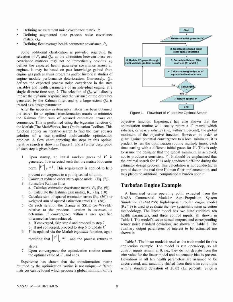
After the necessary system information has been obtained, the search for an optimal transformation matrix to minimize the Kalman filter sum of squared estimation errors can commence. This is performed using the lsqnonlin function of the Matlab (The MathWorks, Inc.) Optimization Toolbox. This function applies an iterative search to find the least squares solution of a user-specified multivariable optimization problem. A flow chart depicting the steps in this optimal iterative search is shown in Figure 1, and a further description of each step is given below.

1. Upon startup, an initial random guess of V* is

generated. It is selected such that the matrix Frobenius

norm * 1F

V = . This requirement is applied to help

prevent convergence to a poorly scaled solution. 2. Construct reduced order state-space model, (Eq. (7)). 3. Formulate Kalman filter

a. Calculate estimation covariance matrix, P∞ (Eq. (9)) b. Calculate the Kalman gain matrix, K∞, (Eq. (10))

4. Calculate sum of squared estimation errors (Eq. (36)), or weighted sum of squared estimation errors (Eq. (38))

5. On each iteration the change in SSEE (or WSSEE) relative to the previous iteration is assessed to determine if convergence within a user specified tolerance has been achieved. a. If converged, skip step 6 and proceed to step 7 b. If not converged, proceed to step 6 to update V*

6. V* is updated via the Matlab lsqnonlin function, again

requiring that * 1

FV = , and the process returns to

step 2 7. Upon convergence, the optimization routine returns

the optimal value of V*, and ends.

Experience has shown that the transformation matrix returned by the optimization routine is not unique—different matrices can be found which produce a global minimum of the

StartStart

1. Generate initial guess for V *1. Generate initial guess for V *

2. Construct reduced orderstate-space equations

2. Construct reduced orderstate-space equations

5. Converged?

5. Converged?

3. Formulate Kalman filtermatrices (P∞ and K∞)

3. Formulate Kalman filtermatrices (P∞ and K∞)

4. Calculate (weighted) sum of squared estimation errors

4. Calculate (weighted) sum of squared estimation errors

7. Return optimal V *7. Return optimal V *

EndEnd

6. Update V * guess throughmulti-variable gradient search6. Update V * guess through

multi-variable gradient search

No

Yes

Figure 1.—Flowchart of V* Iterative Optimal Search

objective function. Experience has also shown that the optimization routine will usually return a V* matrix which satisfies, or nearly satisfies (i.e., within 5 percent), the global minimum of the objective function. However, in order to guard against potential convergence to a local minimum, it is prudent to run the optimization routine multiple times, each time starting with a different initial guess for V*. This is only to assure the designer that the global minimum is achieved, not to produce a consistent V*. It should be emphasized that the optimal search for V* is only conducted off-line during the estimator design process. This calculation is not conducted as part of the on-line real-time Kalman filter implementation, and thus places no additional computational burden upon it.

Turbofan Engine Example A linearized cruise operating point extracted from the

NASA Commercial Modular Aero-Propulsion System Simulation (C-MAPSS) high-bypass turbofan engine model (Ref. 9) is used to evaluate the new systematic tuner selection methodology. The linear model has two state variables, ten health parameters, and three control inputs, all shown in Table 1. The model’s seven sensed outputs, and corresponding sensor noise standard deviation, are shown in Table 2. The auxiliary output parameters of interest to be estimated are shown in

Table 3. The linear model is used as the truth model for this

application example. The model is run open-loop, so all control inputs remain at 0, i.e., they do not deviate from the trim value for the linear model and no actuator bias is present. Deviations in all ten health parameters are assumed to be uncorrelated, and randomly shifted from their trim conditions with a standard deviation of ±0.02 (±2 percent). Since a

NASA/TM—2010-216076 9

parameter’s variance is equal to its standard deviation squared, the health parameter covariance matrix, Ph, is defined as a diagonal matrix with all diagonal elements equal to 0.0004.

Next, the estimation accuracy of the systematic approach for selecting Kalman filter tuning parameters will be compared to the conventional approach of selecting a sub-set of health parameters to serve as tuners (the seven health parameters denoted with “*” in Table 1), and the singular value decomposition approach to tuner selection introduced by Litt in Reference 4. Table 4 shows a comparison of the theoretically predicted estimation errors (squared bias, variance, and total squared error) and experimentally obtained squared estimation errors for each of the three tuner selection approaches. T40 and T50 estimation errors are shown in squared degrees Rankine, and Fn and SmLPC estimation errors are shown in squared percent net thrust and squared percent stall margin respectively. The experimental results were obtained through a Monte Carlo simulation analysis where the health parameters varied over a random distribution in accordance with the covariance matrix, Ph. The test cases were concatenated to produce a single time history input which was provided to the C-MAPSS linear discrete state space model given in Eq. (2), with an update rate of 15 ms. Each individual health parameter test case lasted 30 s.

TABLE 1.—STATE VARIABLES, HEALTH

PARAMETERS, AND ACTUATORS State variables Health parameters Actuators

Nf—fan speed Fan efficiency Wf—fuel flow Nc—core speed Fan flow capacity* VSV—variable stator vane LPC efficiency* VBV—variable bleed valve LPC flow capacity HPC efficiency* HPC flow capacity* HPT efficiency* HPT flow capacity* LPT efficiency LPT flow capacity*

*Health parameters selected as tuners in conventional estimation approach, (identical to sub-set of health parameters selected as tuners in Ref. 4) TABLE 2.—SENSED OUTPUTS AND STANDARD DEVIATION

AS PERCENT OF OPERATING POINT TRIM VALUES Sensed output Standard deviation

(%) Nf—fan speed .......................................................................................... 0.25 Nc—core speed ........................................................................................ 0.25 P24—HPC inlet total pressure ................................................................. 0.50 T24—HPC inlet total temperature ........................................................... 0.75 Ps30—HPC exit static pressure ............................................................... 0.50 T30—HPC exit total temperature ............................................................ 0.75 T48—Exhaust gas temperature ................................................................ 0.75

TABLE 3.—ESTIMATED AUXILIARY PARAMETERS

Auxiliary parameter T40—Combustor exit temperature T50—LPT exit temperature Fn—Net thrust SmLPC—LPC stall margin

At the completion of each 30 s test case, the health parameter vector input instantaneously transitioned to the next test case. A total of 375 30 s test cases were evaluated, resulting in an 11,250 s input time history. Three separate Kalman filters were implemented using the three tuner selection approaches. The experimental estimation errors were determined by calculating the mean squared error between estimated and actual values during the last 10 s of each 30 s test case. The error calculation is based on only the last 10 s so that engine model outputs and Kalman estimator outputs have reached a quasi-steady-state operating condition prior to calculating the error. This ensures that the experimental results are consistent with the theoretically predicted estimation errors which were derived assuming steady-state operation.

From Table 4 it can be seen that the theoretically predicted and the experimentally obtained squared estimation errors exhibit good agreement. If the number of random test cases were increased to a suitably large number, it is expected that the theoretical and experimental results would be identical. It can also be seen that all three estimators are able to produce unbiased estimates of the combustor exit temperature, T40; however, their estimates of LPT exit temperature, T50, net thrust, Fn, and LPC stall margin, SmLPC, are biased. The encouraging finding is that the new systematic approach to tuner selection significantly reduces the overall mean squared estimation error compared to the other two approaches. Relative to the conventional approach of tuner selection the experimental mean squared estimation errors in T40, T50, Fn and SmLPC are reduced 76, 82, 80 and 63 percent, respectively. It can also be observed that the SVD tuner selection approach, which is designed to reduce the estimation error bias, does in fact reduce the sum of squared biases relative to the subset of health parameters approach. However, the SVD approach is also found to increase the estimation variance, which contributes to its overall mean squared estimation error.

TABLE 4.—AUXILIARY PARAMETER SQUARED ESTIMATION ERRORS

Tuners Error T40 (°R)

T50 (°R)

Fn (%)

SmLPC (%)

Subset of health

parameters

Theor. sqr. bias 0.00 561.76 3.84 3.28 Theor. variance 74.76 29.65 0.48 0.34 Theor. sqr. error 74.76 591.41 4.31 3.62 Exper. sqr. error 74.90 583.29 4.27 3.60

SVD tuner selection


Systematic tuner

selection


A visual illustration of the effect that tuner selection has on

Kalman filter estimation accuracy can be seen in Figures 2 through 5, which show actual and estimated results for the auxiliary parameters T40, T50, Fn and SmLPC respectively.

NASA/TM—2010-216076 10

Each plot shows a 300 s segment of the evaluated test cases. The step changes that can be observed in each plot every 30 s correspond to a transition to a different health parameter vector. True model auxiliary parameter outputs are shown in black, and Kalman filter estimates are shown in red. In each figure the information is arranged top to bottom according to tuner selection based upon: a) a subset of health parameters; b) singular value decomposition; and c) the new systematic selection strategy. The information shown in these figures corroborates the information in Table 4; namely all three tuner selection approaches produce unbiased estimates of T40 (Figure 2), while the systematic tuner selection strategy yields a noticeable reduction in the total squared estimation error (squared bias plus variance) of all four auxiliary parameters.

Comparison with Maximum a Posteriori Estimation

The presented systematic tuner selection strategy minimizes the mean squared error of the on-line estimator at steady-state operating conditions, taking advantage of prior knowledge of engine health parameter distributions. As such it is somewhat analogous to the maximum a posteriori (MAP) estimation method which is commonly applied for ground-based aircraft gas turbine engine gas path analysis (Refs. 5 and 6). This leads to the question, how does the on-line Kalman filter estimation accuracy compare to MAP estimation accuracy? Prior to making this comparison the mathematical formulation of the MAP estimator is briefly introduced. Here a steady-state model of the measurement process in the following form is applied

k k ky Hh v= + (39)

where the matrix H relates the effects of the health parameter vector, h, to the sensed measurements, y. From Eq. (19), it can be seen that H is equivalent to C(I – A)–1L + M. The maximum a posteriori (MAP) estimator follows the closed form expression

( ) 11 1 1ˆ T Tk khh P H R H H R y

−− − −= + (40)

The MAP estimator is capable of estimating more unknowns than available measurements due to the inclusion of a priori knowledge of the estimated parameter covariance, Ph. However, the MAP estimator, unlike a Kalman filter, is not a recursive estimator and does not take advantage of past measurements to enhance its estimate at the current time step. Furthermore, the MAP estimator only considers a static relationship between system state variables and measured outputs—it does not consider system dynamics. Because of these differences a Kalman estimator with optimally selected tuning parameters should outperform the MAP estimator. However, under steady-state conditions, with minimal sensor noise the two estimation approaches should produce similar

results. To test this theory, a MAP estimator was designed and its estimation accuracy was compared to a Kalman filter with tuning parameters optimally selected to minimize the estimation errors in the health parameter vector h. First, the two estimators were designed and evaluated using the original sensor noise levels shown in Table 2. Next, the sensor noise levels were set to 1/20th of their original levels, the estimators were re-designed, and the comparison was repeated. Monte Carlo simulation evaluations as previously described were applied (i.e., 375 random health parameter vectors, 30 s in duration, with estimation accuracy calculations based upon the last 10 s of each 30 s test case). Theoretical and experimental estimation errors are shown in Table 5 and Table 6 for the original noise and reduced noise levels, respectively. At original noise levels the Kalman estimator is able to produce smaller estimation errors. However, at the reduced noise level the two estimation approaches are found to be nearly identical. This comparison validates that the Kalman estimation approach is indeed producing a minimum mean squared estimation error as intended, while providing the capability to support real-time on-line estimation under dynamic operating scenarios.

Figure 2.—T40 estimation (tuner comparison).

Figure 3.—T50 estimation (tuner comparison).

0 50 100 150 200 250 300

−500

50

Δ ° R

Subset of health parameters

0 50 100 150 200 250 300

−500

50

Δ ° R

SVD tuner selection

0 50 100 150 200 250 300

−500

50

Δ ° R

time (sec)

Systematic tuner selection

EstimateActual

0 50 100 150 200 250 300

−500

50

Δ ° R


0 50 100 150 200 250 300

−500

50

Δ ° R

SVD tuner selection

0 50 100 150 200 250 300

−500

50

Δ ° R

time (sec)


EstimateActual

NASA/TM—2010-216076 11

Figure 4.—Fn estimation (tuner comparison).

Figure 5.—SmLPC estimation (tuner comparison).

TABLE 5.—HEALTH PARAMETER PERCENT SQUARED ESTIMATION ERRORS (NOMINAL NOISE) Estimator Error type h1 h2 h3 h4 h5 h6 h7 h8 h9 h10 Sum

Kalman filter

Theor. squared bias 1.26 1.48 2.28 1.22 0.00 0.00 0.74 0.00 1.97 3.06 12.00 Theor. variance 0.73 0.19 0.80 0.45 0.40 0.68 0.21 0.21 0.34 0.08 4.09 Theor. squared error 2.00 1.67 3.07 1.66 0.40 0.68 0.96 0.21 2.32 3.14 16.09 Exper. squared error 1.82 1.60 2.77 1.59 0.41 0.68 0.97 0.21 2.13 3.15 15.31

MAP estimator


TABLE 6.—HEALTH PARAMETER PERCENT SQUARED ESTIMATION ERRORS (REDUCED NOISE) Estimator Error type h1 h2 h3 h4 h5 h6 h7 h8 h9 h10 Sum

Kalman filter


MAP estimator


Discussion

While the systematic tuner selection approach presented here appears promising for on-line Kalman filter based parameter estimation applications, there are several practical considerations which need to be assessed when applying such a technique. The optimization routine attempts to minimize the overall squared estimation error—both bias and variance—under steady-state operating conditions. The minimization of the estimation variance in particular can come at the expense of dynamic responsiveness of the Kalman filter. To illustrate this consider the time history plots of actual versus estimated T40 shown in Figure 6. The top plot shows Kalman filter estimation results using a tuning parameter vector

systematically selected to minimize the error in four auxiliary parameters (T40, T50, Fn and SmLPC) as presented in the previous section. The bottom plot shows Kalman filter estimation results using a tuning parameter vector systematically selected to minimize the estimation error in T40 only. At time 100 s a step change in the health parameter input vector is introduced into the engine model; this allows the dynamic response of the two estimators to be compared. It can be observed that T40 estimation variance in the bottom plot is reduced, as is the mean steady-state estimation error (> 300 s). This is not surprising since one would generally expect improved results when optimizing to minimize the error in a single parameter, as opposed to multiple parameters. However, the estimator shown in the

0 50 100 150 200 250 300−10

0

10

Δ %

Fn


0 50 100 150 200 250 300−10

0

10

Δ %

Fn

SVD tuner selection

0 50 100 150 200 250 300−10

0

10

Δ %

Fn

time (sec)


EstimateActual

0 50 100 150 200 250 300−10

0

10

Δ %

Sm


0 50 100 150 200 250 300−10

0

10

Δ %

Sm

SVD tuner selection

0 50 100 150 200 250 300−10

0

10

Δ %

Sm

time (sec)


EstimateActual

NASA/TM—2010-216076 12

Figure 6.—Illustration of tuner impact on estimator response.

bottom plot does require a significantly longer time to reach steady-state convergence. Conversely, the estimator designed to minimize the steady-state error in four auxiliary parameters (top plot) is unable to place as much emphasis on T40 estimation variance reduction, but it is able to track dynamic changes in T40 more rapidly. This example illustrates the inter-dependence between estimation variance and responsiveness. Therefore, it is prudent for a designer to evaluate the Kalman filter to ensure that it tracks engine dynamics acceptably. If the dynamic response is unacceptable, the optimization routine can be rerun placing more weight on estimation error bias reduction, and less weight on variance reduction.

All results presented in this paper are based on a turbofan engine linear state-space model at a single operating point. While this linear assessment enables experimental validation of theoretical predictions, it is not representative of actual aircraft gas turbine engine operation which is a transient non-linear system operating over a broad range of operating conditions. In order for the presented approach to be applicable it would need to be able to produce an optimal set of tuning parameters, not just at a single operating point but rather a globally optimal tuning parameter vector universally applicable over the range of operating conditions that an engine is expected to experience. A potential approach to selecting a single “globally optimal” tuning parameter vector is to modify the optimization routine to minimize the combined estimation error over multiple engine operating points such as takeoff, climb and cruise. This would be a straightforward modification to the Matlab optimization routine, but it would increase the computational time required to calculate the result. Since the systematic tuner selection process is only envisioned to be done once during the system design process, this will not impact the on-line execution

speed of the Kalman filter. It is anticipated that the application of globally optimal tuners will result in some estimation accuracy degradation relative to tuners optimized for individual operating points, although this has not yet been verified or quantified.

Conclusions A systematic approach to tuning parameter selection for on-

line Kalman filter based parameter estimation has been presented. This technique is specifically applicable for the underdetermined aircraft engine parameter estimation case where there are fewer sensor measurements than unknown health parameters which will impact engine outputs. It creates and applies a linear transformation matrix, V*, to select a vector of tuning parameters which are a linear combination of all health parameters. The tuning parameter vector is selected to be of low-enough dimension to be estimated, while minimizing the mean-squared error of Kalman filter estimates. The multi-parameter iterative search routine applied to optimally select V* was presented. Results have shown that while the transformation matrix returned by the optimization routine is not unique (different matrices can be found which produce a global minimum of the objective function), the routine is effective in returning a transformation matrix which is optimal, or near optimal, regardless of its initial starting guess of the matrix. The efficacy of the systematic approach to tuning parameter selection was demonstrated by applying it to parameter estimation in an aircraft turbofan engine linear point model. It was found to significantly reduce mean squared estimation errors compared to the conventional approach of selecting a subset of health parameters to serve as tuners. In some parameters the mean squared estimation error reduction was found to be over 80 percent. These estimation improvements were theoretically predicted and experimentally validated through Monte Carlo simulation studies.

The systematic approach to Kalman filter design is envisioned to be applicable for a broad range of on-board aircraft engine model-based applications which produce estimates of unmeasured parameters. This includes model-based controls, model-based diagnostics, and on-board life usage algorithms. It is also envisioned to have benefits for sensor selection during the engine design process, specifically for assessing the performance estimation accuracy benefits of different candidate sensor suites. Areas for future work include extending the technique to produce a tuning parameter vector optimal over a range of operating conditions, and evaluating the technique on a non-linear engine model, under both steady-state and transient operating conditions.

References

1. Luppold, R.H. Roman, J.R., Gallops, G.W., Kerr, L.J., (1989), “Estimating In-Flight Engine Performance Varaiations Using Kalman Filter Concepts,” AIAA-89-2584, AIAA 25th Joint Propulsion Conference.

0 100 200 300 400 500 600−50

0

50

100

150

200

Δ ° R

Tuners selected to minimize T40, T50, Fn and SmLPC error

0 100 200 300 400 500 600−50

0

50

100

150

200

Δ ° R

Tuners selected to minimize T40 error

time (sec)

EstimateActual

NASA/TM—20 0-216076 13

2. Volponi, A., (2008), “Enhanced Self-Tuning On-Board Real-

Time Model (eSTORM) for Aircraft Engine Performance Health Tracking,” NASA/CR—2008-215272.

3. Kumar, A., Viassolo, D., (2008), “Model-Based Fault Tolerant Control,” NASA/CR—2008-215273.

4. Litt, J.S., (2008), “An Optimal Orthogonal Decomposition Method for Kalman Filter-Based Turbofan Engine Thrust Estimation,” Journal of Engineering for Gas Turbines and Power, Vol. 130/011601–1.

5. Doel, D.L., (1994), “An Assessment of Weighted-Least-Squares-Based Gas Path Analysis,” J. of Engineering for Gas Turbines and Power, Vol. 116, pp. 336–373.

6. Volponi, A.J., et al, (2003), “Gas Turbine Condition Monitoring

and Fault Diagnostics”, Von Karman Institute for Fluid Dynamics, Lecture Series 2003–01.

7. España, M.D., (1994), “Sensor Biases Effect on the Estimation Algorithm for Performance-Seeking Controllers,” J. Propulsion and Power, 10, pp. 527–532.

8. Simon, D., (2006), “Optimal State Estimation, Kalman, H∞, and Nonlinear Approaches,” John Wiley & Sons, Inc., Hoboken, NJ.

9. Frederick, D.K., DeCastro, J.A., Litt, J.S., (2007), “User’s Guide for the Commercial Modular Aero-Propulsion System Simulation (C-MAPSS),” NASA/TM—2007-215026.

1

REPORT DOCUMENTATION PAGE Form Approved OMB No. 0704-0188

The public reporting burden for this collection of information is estimated to average 1 hour per response, including the time for reviewing instructions, searching existing data sources, gathering and maintaining the data needed, and completing and reviewing the collection of information. Send comments regarding this burden estimate or any other aspect of this collection of information, including suggestions for reducing this burden, to Department of Defense, Washington Headquarters Services, Directorate for Information Operations and Reports (0704-0188), 1215 Jefferson Davis Highway, Suite 1204, Arlington, VA 22202-4302. Respondents should be aware that notwithstanding any other provision of law, no person shall be subject to any penalty for failing to comply with a collection of information if it does not display a currently valid OMB control number. PLEASE DO NOT RETURN YOUR FORM TO THE ABOVE ADDRESS. 1. REPORT DATE (DD-MM-YYYY) 01-01-2010

2. REPORT TYPE Technical Memorandum

3. DATES COVERED (From - To)

4. TITLE AND SUBTITLE Optimal Tuner Selection for Kalman Filter-Based Aircraft Engine Performance Estimation

5a. CONTRACT NUMBER

5b. GRANT NUMBER

5c. PROGRAM ELEMENT NUMBER

6. AUTHOR(S) Simon, Donald, L.; Garg, Sanjay

5d. PROJECT NUMBER

5e. TASK NUMBER

5f. WORK UNIT NUMBER WBS 645846.02.07.03.03.012

7. PERFORMING ORGANIZATION NAME(S) AND ADDRESS(ES) National Aeronautics and Space Administration John H. Glenn Research Center at Lewis Field Cleveland, Ohio 44135-3191

8. PERFORMING ORGANIZATION REPORT NUMBER E-17111

9. SPONSORING/MONITORING AGENCY NAME(S) AND ADDRESS(ES) National Aeronautics and Space Administration Washington, DC 20546-0001

10. SPONSORING/MONITOR'S ACRONYM(S) NASA

11. SPONSORING/MONITORING REPORT NUMBER NASA/TM-2010-216076; GT2009-59684

12. DISTRIBUTION/AVAILABILITY STATEMENT Unclassified-Unlimited Subject Category: 07 Available electronically at http://gltrs.grc.nasa.gov This publication is available from the NASA Center for AeroSpace Information, 443-757-5802

13. SUPPLEMENTARY NOTES

14. ABSTRACT A linear point design methodology for minimizing the error in on-line Kalman filter-based aircraft engine performance estimation applications is presented. This technique specifically addresses the underdetermined estimation problem, where there are more unknown parameters than available sensor measurements. A systematic approach is applied to produce a model tuning parameter vector of appropriate dimension to enable estimation by a Kalman filter, while minimizing the estimation error in the parameters of interest. Tuning parameter selection is performed using a multi-variable iterative search routine which seeks to minimize the theoretical mean-squared estimation error. This paper derives theoretical Kalman filter estimation error bias and variance values at steady-state operating conditions, and presents the tuner selection routine applied to minimize these values. Results from the application of the technique to an aircraft engine simulation are presented and compared to the conventional approach of tuner selection. Experimental simulation results are found to be in agreement with theoretical predictions. The new methodology is shown to yield a significant improvement in on-line engine performance estimation accuracy. 15. SUBJECT TERMS Aircraft engines; Systems health monitoring; Gas turbine engines; Kalman filtering; State estimation

16. SECURITY CLASSIFICATION OF: 17. LIMITATION OF ABSTRACT UU

18. NUMBER OF PAGES

19

19a. NAME OF RESPONSIBLE PERSON STI Help Desk (email:[email protected])

a. REPORT U

b. ABSTRACT U

c. THIS PAGE U

19b. TELEPHONE NUMBER (include area code) 443-757-5802

Standard Form 298 (Rev. 8-98)Prescribed by ANSI Std. Z39-18

Optimal Tuner Selection for Kalman Filter-Based … · Donald L. Simon and Sanjay Garg Glenn...

Documents

Transcript of Optimal Tuner Selection for Kalman Filter-Based … · Donald L. Simon and Sanjay Garg Glenn...