Electronic copy available at: http://ssrn.com/abstract=2551870

Optimal Trading Strategies Based on Multivariate Regression Results

idemahK demaH

Abstract:

The main purpose of this paper is to efficiently utilize the forecasts made by multivariate linear

regression analysis. To this end, we build up a mathematical model for the trading decisions based on the

regression results. Given that these results are uncertain, we seek to maximize the expected profits

acquired through opening and closing trade positions. To find the best trading strategy, a dynamic

programming approach has been employed. In this sense, we firstly find optimal take profit levels

associated with opening buy and sell positions. Then we decide to buy, sell or wait, based on the

maximum profit we are going to expect in each case. To show how this method works we apply our

approach to finding the optimal strategy for trading GBPUSD rate based on a multivariate regression

model fitted to the historical daily data on the FOREX Market.

Keywords:

Forecasting, Multivariate Regression, Trade Position, Take Profit, Financial Market, Optimal Decision

Electronic copy available at: http://ssrn.com/abstract=2551870

1. Introduction

The ability to accurately forecast in financial markets is a vital part of modern business management.

Arguably, it is sufficient to use the past and existing price observations to make predictions about future

price movements. In contrast, Fama (1965) states that according to the theory of random walks, the future

path of the price level of a security is no more predictable than the path of a series of cumulated random

numbers. This implies that the past cannot be used to predict the future in any meaningful way. In the

immediate term, the random-walk model of foreign exchange rates, suggests that the best predictor of

tomorrow’s exchange rate is the current exchange rate.

On the other hand, various empirical studies have documented substantial evidence on the

predictability of asset returns. Their studies suggest that asset returns are correlated, and hence,

predictability can be captured to some degree, by certain statistical models. Treynor and Ferguson (1984)

demonstrated theoretically that past prices, combined with other (past) information, can predict the future

price movements. Likewise, numerous empirical studies, however, suggest that foreign-currency returns

may not be independent nor conform to a stable probability distribution. Ellis and Wilson (2005) suggest

some method that yields forecasts superior to those of a random walk model. In other words history

repeats itself in that "patterns" of past Market behavior will tend to recur in the future.

However the prime objective of this study is to suggest a decision model for trading based on the

uncertain forecast results. According to the framework developed by Neftci (1991), a well-defined trading

rule should be a Markov time, i.e. it should use only information available up to current moment for its

construction. We utilize and refer to this information as independent variables. Particularly our approach

to the forecasting is Multivariate Multiple Regression, which is a study on the relationship between few

dependent variables and many independent variables.

The discussion between different types of trades is explained by different principles and relationships

that are used for trading. They contain indicators covering all buy/sell rules that are formulated on the

basis of the well-defined mathematical expressions. Most trading rules have been developed on the basis

of the empirical observations, rather than derived or modeled mathematically. At the same time, fewer

Electronic copy available at: http://ssrn.com/abstract=2551870

studies concentrate on the development of the theoretical framework for the analysis and optimization of

the trading rules, although there is a pool of users (traders), who create the demand for this type of

research. Thus, in this paper, we concentrate on mathematical investigation to model and optimize trading

strategies based on the forecasting results. They will be formalized and explained from the point of view

of the multivariate statistical theory.

Our main analysis focuses on two questions: Firstly, under what conditions should we buy, sell or

wait? Secondly, how much profit should we expect from a trade and thus what take profit limits should

we put on a position? In this sense we define three response variables to be predicted by means of a

regression model. These are the Maximum, Minimum and Closing prices/rates in one period ahead in our

timeframe. In order to demonstrate how this method can be useful in practical situations, we applied it to

provide optimal trading strategies for GBPUSD exchange rate, based on the regression model stated in the

appendix. The data used in this study are the exchange rates downloaded from Meta-Quotes Corp. It

includes all the dependent and independent variables required in the regression model.

The paper is organized as follows. In the next section, a mathematical model is presented to derive

optimal trading strategies based on multivariate regression forecasts. In section 2 a simple numerical case

illustrates how to put the model into practice. This sample analysis is based on the regression model

presented in the appendix. Finally Section 4 presents the concluding remarks and suggests some

extensions for future research.

2. Trading Strategy and Decision Model

The fundamental and simple rule of profitable trading is to buy cheaper and sell dearer. Thus, the

entire trading activities at financial markets come to the successive operations performed to sell or buy

securities. To do so, one has to open, and close trade positions. Trade position is a market commitment,

which can be opened by a brokerage company at an order initiated by the trader. To open a trade position,

one has to make a transaction, and to close a position, one has to make an inverse operation. A critical

factor for successful trading is the ability to determine the exit points for any trade position. There can be

values of the Stop Loss and Take Profit order levels attached to an open position. Positions can be closed

on the trader's demand or at execution of Stop Loss or Take Profit orders.

There are two prices (rates) , at which the position will be closed automatically if the security price

reaches any of those levels. Take Profit is a close order which is intended for gaining profit if the security

price reaches that level. It is a price (rate) set by trader, at which a market position will be closed when

this level of profit is produced for the position. This order is always connected to an open position and its

execution results in closing of the position. Stop Loss is also a close order used for minimizing of losses if

the security price (rate) has started to move in an unprofitable direction.

To reach a manageable model and make a practical contribution, this paper focuses on a particular

situation in which we are about to open a position in a specific time (e.g. 10:00am

), for a particular

financial instrument (e.g. GBPUSD). At this moment, we have three choices to decide: Buy, Sell or Wait?

If we open a position (Buy or Sell), we have to decide when to exit that position, which is the Take Profit

level we attach to the position as the closing criterion. In one hand we wish to gain the largest profit from

an order, and on the other hand a lower Take Profit level will be more likely to be met. Besides, we are

willing to hold any position for a limited time interval (e.g. one hour: 10 to 11) and if we don’t meet the

take profit level during that period, we will close the position at its end.

This approach also sheds light on what to forecast. Actually we need to decide based on the

forecasted values in the upcoming time interval. Since we are willing to attach a Take Profit level to the

orders and the trades are two-sided (buy/sell), we found the most useful values to forecast are the High,

Low and Closing prices (rates) in the time interval which we may hold the position. Therefore, hereby we

define three (random) variables to forecast in one upcoming period:

Y1 = Highest Upcoming Rate – Current Rate = High (imminent candle) – Open (imminent candle)

Y2 = Current Rate – Lowest Upcoming Rate = Open (imminent candle) – Low (imminent candle)

Y3 = Upcoming Closing Rate – Current Rate = Close (imminent candle) – Open (imminent candle)

Noticeably, Y1 and Y2 are nonnegative, but Y3 can take any real value. Meanwhile we assume that

half the times, the Low happens before High and half the times the reverse happens. Then we can

formulate our decision problem in mathematical terms as follows:

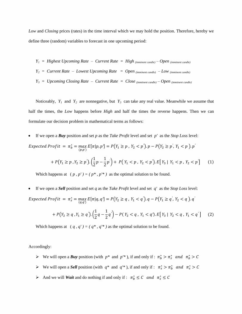
If we open a Buy position and set p as the Take Profit level and set p' as the Stop Loss level:

𝐸𝑥𝑝𝑒𝑐𝑡𝑒𝑑 𝑃𝑟𝑜𝑓𝑖𝑡 = 𝜋𝑏∗ = 𝑚𝑎𝑥

(𝑝,𝑝′)𝐸[𝜋|𝑝, 𝑝′] = 𝑃(𝑌1 ≥ 𝑝 , 𝑌2 < 𝑝′). 𝑝 − 𝑃(𝑌2 ≥ 𝑝′, 𝑌1 < 𝑝 ). 𝑝′

+ 𝑃(𝑌1 ≥ 𝑝 , 𝑌2 ≥ 𝑝′). (1

2𝑝 −

1

2𝑝′) + 𝑃( 𝑌1 < 𝑝 , 𝑌2 < 𝑝′). 𝐸[ 𝑌3 | 𝑌1 < 𝑝 , 𝑌2 < 𝑝′] (1)

Which happens at ( p , p' ) = ( p* , p'* ) as the optimal solution to be found.

If we open a Sell position and set q as the Take Profit level and set q' as the Stop Loss level:

𝐸𝑥𝑝𝑒𝑐𝑡𝑒𝑑 𝑃𝑟𝑜𝑓𝑖𝑡 = 𝜋𝑠∗ = 𝑚𝑎𝑥

(𝑞,𝑞′)𝐸[𝜋|𝑞, 𝑞′] = 𝑃(𝑌2 ≥ 𝑞 , 𝑌1 < 𝑞′). 𝑞 − 𝑃(𝑌1 ≥ 𝑞′, 𝑌2 < 𝑞 ). 𝑞′

+ 𝑃(𝑌2 ≥ 𝑞 , 𝑌1 ≥ 𝑞′). (1

2𝑞 −

1

2𝑞′) − 𝑃( 𝑌2 < 𝑞 , 𝑌1 < 𝑞′). 𝐸[ 𝑌3 | 𝑌2 < 𝑞 , 𝑌1 < 𝑞′ ] (2)

Which happens at ( q , q' ) = ( q* , q'* ) as the optimal solution to be found.

Accordingly:

We will open a Buy position (with p* and p'* ), if and only if : 𝜋𝑏∗ > 𝜋𝑠

∗ 𝑎𝑛𝑑 𝜋𝑏∗ > 𝐶

We will open a Sell position (with q* and q'* ), if and only if : 𝜋𝑠∗ > 𝜋𝑏

∗ 𝑎𝑛𝑑 𝜋𝑠∗ > 𝐶

And we will Wait and do nothing if and only if : 𝜋𝑏∗ ≤ 𝐶 𝑎𝑛𝑑 𝜋𝑠

∗ ≤ 𝐶

Where, C stands for the cost of a single trade (opening and closing a position), comprising the

Commissions, the Spreads, and the Risk premiums we are to be guarded.

Hereafter we assume to have enough margins corresponding to our trading timeframe, so that we are

able to tolerate any fluctuations in our specific time interval. Thus we don’t consider the Stop Loss level

and focus on the optimal Take Profit as the closing criterion1. So the problems (1) and (2) will be

rewritten as follows:

If we open a Buy position and set p as the take profit level:

𝐸𝑥𝑝𝑒𝑐𝑡𝑒𝑑 𝑃𝑟𝑜𝑓𝑖𝑡 = 𝜋𝑏∗ = 𝑚𝑎𝑥

𝑝𝐸[𝜋|𝑝] = 𝑃(𝑌1 ≥ 𝑝). 𝑝 + 𝑃( 𝑌1 < 𝑝). 𝐸[ 𝑌3 | 𝑌1 < 𝑝] (3)

Happening at p = p*.

If we open a Sell position and set q as the take profit level:

𝐸𝑥𝑝𝑒𝑐𝑡𝑒𝑑 𝑃𝑟𝑜𝑓𝑖𝑡 = 𝜋𝑠∗ = 𝑚𝑎𝑥

𝑞𝐸[𝜋|𝑞] = 𝑃(𝑌2 ≥ 𝑞). 𝑞 − 𝑃(𝑌2 < 𝑞). 𝐸[ 𝑌3 | 𝑌2 < 𝑞] (4)

Happening at q = q*.

Consequently:

We will open a Buy position (with p = p* ) if and only if 𝜋𝑏∗ > 𝑚𝑎𝑥 {𝜋𝑠

∗ , 𝐶}

We will open a Sell position (with q = q* ) if and only if 𝜋𝑠∗ > 𝑚𝑎𝑥 {𝜋𝑏

∗ , 𝐶}

And we will Wait and do nothing if and only if 𝐶 ≥ 𝑚𝑎𝑥 {𝜋𝑠∗ , 𝜋𝑏

∗}

Now, to proceed further we consider using multivariate regression method to forecast a new response

Y0 = (Y1 ,Y2 ,Y3 ), and the residuals show a Normal behavior. Thus we will have a tri-variate Normal

distribution for the predicted vector Y0 , as follows:

𝒀 ∼ 𝑁3 ( �̂� = [

�̂�1

�̂�2

�̂�3

] , 𝑺 = [

�̂�11 �̂�12 �̂�13

�̂�12 �̂�22 �̂�23

�̂�13 �̂�23 �̂�33

] ) (5)

1 Actually the genuine basis for this decision is the infinitely large optimal stop loss levels suggested through

numerical solution of those equations (i.e. Simulation, Monte Carlo).

In which, from multivariate statistical theory we have:

�̂� = �̂�′. 𝒙𝟎 and 𝑺 = (1 + 𝒙𝟎′ (𝑿′𝑿)

−1𝒙𝟎) �̂� (6)

Where,

We have r predictor variables and n (training) observations,

X is the n*(r+1) design matrix,

�̂� is the (r+1)*3 vector of estimated regression parameters,

x0 is the current values of predictor variables, (r+1)*1, and

�̂� =�̂�′�̂�

𝑛−𝑟−1 is the 3*3 covariance matrix of residuals regarding �̂� as the n*3 matrix of residuals.

Anyway, returning to the notations used in (3), we can easily find out that:

𝐸[ 𝑌3 | 𝑌1 < 𝑝] =

1

𝜑 (𝑝 − 𝜇1

√𝜎11)

. ∫ ∫ 𝑦3 . 𝑓13(𝑦1, 𝑦3) . 𝑑𝑦1𝑑𝑦3

𝑝

𝑦1=−∞

+∞

𝑦1=−∞

= 𝜇3 −𝜎13

𝜑 (𝑝 − 𝜇1

√𝜎11)

.1

√2𝜋. 𝜎11

. 𝑒−(𝑝−𝜇1)2

2𝜎11 (7)

𝐸[ 𝑌3 | 𝑌2 < 𝑞] =

1

𝜑 (𝑞 − 𝜇2

√𝜎22)

. ∫ ∫ 𝑦3 . 𝑓23(𝑦2, 𝑦3) . 𝑑𝑦2𝑑𝑦3

𝑞

𝑦2=−∞

+∞

𝑦2=−∞

= 𝜇3 −𝜎23

𝜑 (𝑞 − 𝜇2

√𝜎22)

.1

√2𝜋. 𝜎22

. 𝑒−(𝑞−𝜇2)2

2𝜎22 (8)

In which, f13 and f23 are the bi-variate Normal probability density functions as follows respectively:

𝑁2 ([�̂�1

�̂�3] , [

�̂�11 �̂�13

�̂�13 �̂�33]) 𝑁2 ([

�̂�2

�̂�3] , [

�̂�22 �̂�23

�̂�23 �̂�33])

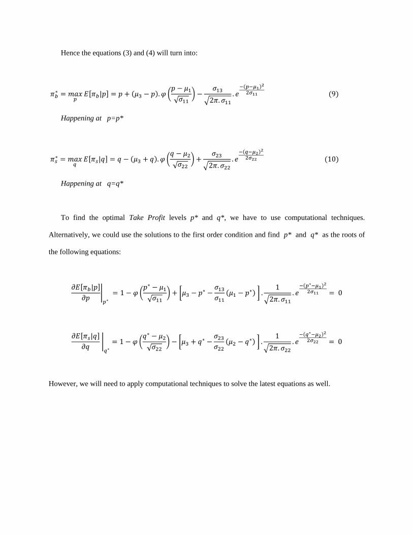
Hence the equations (3) and (4) will turn into:

𝜋𝑏∗ = 𝑚𝑎𝑥

𝑝𝐸[𝜋𝑏|𝑝] = 𝑝 + (𝜇3 − 𝑝). 𝜑 (

𝑝 − 𝜇1

√𝜎11) −

𝜎13

√2𝜋. 𝜎11

. 𝑒−(𝑝−𝜇1)2

2𝜎11 (9)

Happening at p=p*

𝜋𝑠∗ = 𝑚𝑎𝑥

𝑞𝐸[𝜋𝑠|𝑞] = 𝑞 − (𝜇3 + 𝑞). 𝜑 (

𝑞 − 𝜇2

√𝜎22) +

𝜎23

√2𝜋. 𝜎22

. 𝑒−(𝑞−𝜇2)2

2𝜎22 (10)

Happening at q=q*

To find the optimal Take Profit levels p* and q*, we have to use computational techniques.

Alternatively, we could use the solutions to the first order condition and find p* and q* as the roots of

the following equations:

𝜕𝐸[𝜋𝑏|𝑝]

𝜕𝑝|

𝑝∗

= 1 − 𝜑 (𝑝∗ − 𝜇1

√𝜎11) + [𝜇3 − 𝑝∗ −

𝜎13

𝜎11

(𝜇1 − 𝑝∗) ] .1

√2𝜋. 𝜎11

. 𝑒−(𝑝∗−𝜇1)2

2𝜎11 = 0

𝜕𝐸[𝜋𝑠|𝑞]

𝜕𝑞 |

𝑞∗

= 1 − 𝜑 (𝑞∗ − 𝜇2

√𝜎22) − [𝜇3 + 𝑞∗ −

𝜎23

𝜎22

(𝜇2 − 𝑞∗) ] .1

√2𝜋. 𝜎22

. 𝑒−(𝑞∗−𝜇2)2

2𝜎22 = 0

However, we will need to apply computational techniques to solve the latest equations as well.

3. Numerical Example

To see how the expected profit behaves, we use the regression model explained in the appendix to

find an optimal trading strategy for GBPUSD at 10:00am

in July, 19th 2010. This model forecasts the

values (in pips) of the response variables to be ŷ1 = 10, ŷ2 = 98, and ŷ3 = +5.2. Also using the covariance

matrix of residuals along equation (6), we have for this observation:

𝑺 = (1 + 𝒙𝟎′ (𝑿′𝑿)

−1𝒙𝟎) �̂� = [

. 𝟑𝟔 −. 𝟐𝟓 . 𝟒𝟕−. 𝟐𝟓 . 𝟓𝟔 −. 𝟔𝟑. 𝟒𝟕 −. 𝟔𝟑 𝟏. 𝟎𝟒

] ∗ 𝟏𝟎−𝟒

Now we employ equations (9) and (10) to find the optimal trading strategy. As figure 1 illustrates, the

maximum expected profit is about 13 pips, which is associated to a sell position with take profit level

equal to 88.5 pips. Actually if we meet this limit we expect to gain +88.5 pips, and otherwise we expect to

lose 5 pips down to closing at 11am

. As a matter of fact, this take profit limit was not met and the actual

profit was +37 pips, due to the realized Closing rate at 11am

. (Real Low rate = 53 < take profit = 88.5)

Figure 1 – Expected profits for trading strategies in July, 19th

, 2010

4. Conclusion

To make money in the financial markets, most of the traders base their strategies on the forecasts.

Forecasts may be used in numerous ways and we try to use them most effectively. In this study we have

primarily focused on finding the optimal take profit levels based on the forecasts derived from

multivariate regression analysis. To this end, we applied probability theory and built up a mathematical

model to maximize the expected net (cumulative) profits gained through opening and closing positions.

Finally we come to such complex equations that cannot be solved analytically and we rely on the

computational techniques to achieve the optimal solutions.

Taking a Dynamic Programming approach, we suggest a trading strategy based on the outcomes of

our mathematical model. In this sense we firstly find the maximum expected profit assuming we open a

Buy position and compare it to the maximum expected profit in case of the Sell position. Based on which

one being larger, we decide to buy or sell, except when this larger profit is less than the costs incurred by

the trade, in which we suspend opening any position and wait for the next trading opportunity.

In order to illustrate how one can use this method to make profitable trades, we found the numerical

solution for a sample case which was based on a regression model developed in the appendix. Suggesting

that overall, using this method, we may make lucrative trading decisions, even having employed a very

simple regression model with poor predictive ability.

For researchers interested in applying this method to more efficient regression models, we

recommend including some nonlinear combinations of the rate ratios and volume data. For instance, one

may consider the quadratic combinations, reciprocals and squared roots in the regression model. This may

substantially improve the accuracy of classifying trades in general. Also one may extend the application

of this method to other (more suitable and advanced) models like robust and moving regression models as

Preminger and Franck (2007) examine, or autoregressive models based on time series approaches as Fang

and Xu (2003) consider. Clearly the covariance matrices mentioned in the previous section are essential to

estimate the prediction intervals and find the optimal solutions.

Appendix: Empirical Study, Variable Definition, and Regression

In order to define variables, we presume that in each business day we open a position at 10:00am

, and

close it at 11:00am

if the take profit limit was not met during this one hour period. Therefore, the High,

Low and Closing rates of the 60-minute candle between 10:00am

and 11:00am

describe the response

(dependent) variables. We aim to use historical daily market data to develop a regression model that

forecasts the response variables in this particular hour each day. The data series studied in this paper are

daily-frequency observations on Pound versus US Dollar exchange rate (GBPUSD), as the dependent

variables. Our sample contains trade data for 742 working days between February 1st, 2007 (Thursday)

and January 8th, 2010 (Friday). The transactions data were provided by “Meta-Quotes Software Corp.”.

The predictors are composed of the available data up to 10:00am

(decision point) in each trading day.

To define the independent variables, we consider eight recent 15-minute candles associated with two

hours between 8:00am

and 10:00am

in the trading day for seven symbols: GBPUSD, EURUSD, USDCHF,

USDJPY, USDCAD, AUDUSD and GOLD which are supposed to have some leading information. Thus,

after careful considerations, we have chosen 448 predictor variables from within the Open, High, Low,

Close, Volume, MFI and some other combinations of the data in each 15-minute candle. Needless to say,

the rate variables are meaningless unless compared to the Opening rates at 10:00am

.

An important feature of financial markets is the presence of so-called calendar effects, by which

predictable patterns associated with the month of the year, the day of the week, or the hour of the day

exist in market behavior. For example, Osborne et al. (2008) show that currencies are correlated with each

other in different days of the week. Hence we include 16 time indicators (comprising Year, Month, Day,

Weekday and some functions of them) as additional predictors. Consequently there will be 464 predictor

variables altogether.

To avoid multicollinearity problem and reach a better out of sample predictive ability, we perform a

principal component analysis on our data. Since the data contains very different scales we use the

correlation matrix for PCA. The results suggest the first 300 components contribute 999% of the total

variance. Hence we will proceed to the stepwise regression analysis with the first 300 principal

components. In our stepwise regression, the p-value to enter a variable is 0.05 (based on the F-statistics),

while the p-value to remove it is 0.1. The stepwise regression reduced the number of independent

components to 109. From the Normal probability plots and histograms of the residuals we deduce that all

the three responses have normal error terms. The residual plots against the fitted values show no evidence

of serious departures from the model. The results suggest that the model is fit and appropriate, thus it was

selected for developing trading strategies. Parameter estimations were carried out using MATLAB® with

Mean Square Error (MSE) as the fitness function.

According to the values of R2, the model explains 48.43% of the total variations in Y1, 35.44% of the

total variations in Y2, and 33.55% of the total variations in Y3. Also we can see that R2

adj is 39.54% ,

24.31% and 22.08% for Y1 , Y2 and Y3 respectively.

References

1. Ellis, Craig; Wilson, Patrick; “A stochastic approach to modeling the USD/AUD exchange rate:

Implications for managing foreign exchange exposure”, International Journal of Managerial

Finance, 2005, Vol. 1, No. 1, pp. 36-48.

2. Fama, F. Eugene; “The Behavior of Stock-Market Prices”, Journal of Business, Jan 1965, Vol. 38,

No. 1, pp. 34-105.

3. Fang, Yue; Xu, Daming; “The predictability of asset returns: an approach combining technical

analysis and time series forecasts”, International Journal of Forecasting, 2003, Vol. 19, pp. 369-385

4. Neftci, S. N.; “Naïve trading rules in financial markets and Wiener-Kolmogorov predicition

theory: A study of technical analysis”, Journal of Business, Oct. 1991, Vol. 64, Issue 4, pp. 549-571.

5. Osborne, Denise R.; Savva, Christos S.; Gill, Len; “Periodic Dynamic Conditional Correlations

between Stock Markets in Europe and the US”, Journal of Financial Econometrics, 2008, Vol. 6,

No. 3, pp. 307-325.

6. Preminger, Arie; Raphael, Franck; “Forecasting exchange rates: A robust regression approach”,

International Journal of Forecasting, 2007, Vol. 23, pp. 71-84.

7. Treynor, J.L.; R. Ferguson; “In defence of technical analysis”, Journal of Finance, July 1985, Vol.

40, No. 3, pp.757-773.

8. Zuhaimy, Ismail; A. Yahya; A. Shabri; “Forecasting Gold Prices Using Multiple Linear Regression

Method”, American Journal of Applied Sciences, 2009, Vol. 6 (8), pp. 1509-1514.