Optimal Trading Algorithms
127
Diss. ETH No. 17746 Optimal Trading Algorithms: Portfolio Transactions, Multiperiod Portfolio Selection, and Competitive Online Search A dissertation submitted to the ETH Zürich for the degree of Doctor of Sciences presented by Julian Michael Lorenz Diplom-Mathematiker, Technische Universität München born 19.12.1978 citizen of Germany accepted on the recommendation of Prof. Dr. Angelika Steger, examiner Prof. Dr. Hans-Jakob Lüthi, co-examiner Dr. Robert Almgren, co-examiner 2008
-
Upload
saiprojectwork -
Category
Documents
-
view
22 -
download
1
description
Optimal Trading Algorithms: Portfolio Transactions, Multiperiod Portfolio Selection, and Competitive Online Search
Transcript of Optimal Trading Algorithms
Diss. ETH No. 17746
Optimal Trading Algorithms:Portfolio Transactions, Multiperiod PortfolioSelection, and Competitive Online Search
A dissertation submitted to the
ETH Zürich
for the degree of
Doctor of Sciences
presented by
Julian Michael Lorenz
Diplom-Mathematiker, Technische Universität München
born 19.12.1978
citizen of Germany
accepted on the recommendation of
Prof. Dr. Angelika Steger, examiner
Prof. Dr. Hans-Jakob Lüthi, co-examiner
Dr. Robert Almgren, co-examiner
2008

To my parents
Abstract
This thesis deals with optimal algorithms for trading of financial securities. It is divided into
four parts: risk-averse execution with market impact, Bayesian adaptive trading with price
appreciation, multiperiod portfolio selection, and the generic online search problem k-search.
Risk-averse execution with market impact. We consider the execution of portfolio transac-
tions in a trading model with market impact. For an institutional investor, especially in equity
markets, the size of his buy or sell order is often larger than the market can immediately supply
or absorb, and his trading will move the price (market impact). His order must be worked across
some period of time, exposing him to price volatility. The investor needs to find a trade-off
between the market impact costs of rapid execution and the market risk of slow execution.
In a mean-variance framework, an optimal execution strategy minimizes variance for a specified
maximum level of expected cost, or conversely. In this setup, Almgren and Chriss (2000) give
path-independent (also called static) execution algorithms: their trade-schedules are determin-
istic and do not modify the execution speed in response to price motions during trading.
We show that the static execution strategies of Almgren and Chriss (2000) can be significantly
improved by adaptive trading. We first illustrate this by constructing strategies that update
exactly once during trading: at some intermediary time they may readjust in response to the
stock price movement up to that moment. We show that such single-update strategies yield
lower expected cost for the same level of variance than the static trajectories of Almgren and
Chriss (2000), or lower variance for the same expected cost.
Extending this first result, we then show how optimal dynamic strategies can be computed to any
desired degree of precision with a suitable application of the dynamic programming principle. In
this technique the control variables are not only the shares traded at each time step, but also the
maximum expected cost for the remainder of the program; the value function is the variance of
the remaining program. This technique reduces the determination of optimal dynamic strategies
to a series of single-period convex constrained optimization problems.
The resulting adaptive trading strategies are “aggressive-in-the-money”: they accelerate the exe-
cution when the price moves in the trader’s favor, spending parts of the trading gains to reduce
risk. The relative improvement over static trade schedules is larger for large initial positions,
expressed in terms of a new nondimensional parameter, the market power µ. For small portfolios,
µ→ 0, optimal adaptive trade schedules coincide with the static trade schedules of Almgren and
Chriss (2000).
Bayesian adaptive trading with price appreciation. This part deals with another major
driving factor of transaction costs for institutional investors, namely price appreciation (price
trend) during the time of a buy (or sell) program. An investor wants to buy (sell) a stock before
other market participants trade the same direction and push up (respectively, down) the price.
iii

iv
Thus, price appreciation compels him to complete his trade rapidly. However, an aggressive
trade schedule incurs high market impact costs. Hence, it is vital to balance these two effects.
The magnitude of the price appreciation is uncertain and comes from increased trading by other
large institutional traders. Institutional trading features a strong daily cycle. Market participants
make large investment decisions overnight or in the early morning, and then trade across the
entire day. Thus, price appreciation in early trading hours gives indication of large net positions
being executed and ensuing price momentum. We construct a model in which the trader uses the
observation of the price evolution during the day to estimate price momentum and to determine
an optimal trade schedule to minimize total expected cost of trading. Using techniques from
dynamic programming as well as the calculus of variations we give explicit optimal trading
strategies.
Multiperiod portfolio selection. We discuss the well-known mean-variance portfolio selection
problem (Markowitz, 1952, 1959) in a multiperiod setting. Markowitz’s original model only con-
siders an investment in one period. In recent years, multiperiod and continous-time versions have
been considered and solved. In fact, in a multiperiod setting the portfolio selection problem is
related to the optimal execution of portfolio transactions. Using the same dynamic programming
technique as in the first part of this thesis, we explicitly derive the optimal dynamic investment
strategy for discrete-time multiperiod portfolio selection. Our solution coincides with previous
results obtained with other techniques (Li and Ng, 2000).
Generic online search problem k-search. We discuss the generic online search problem k-
search. In this problem, a player wants to sell (respectively, buy) k ≥ 1 units of an asset with the
goal of maximizing his profit (minimizing his cost). He is presented a series of prices, and after
each quotation he must immediately decide whether or not to sell (buy) one unit of the asset.
We impose only the rather minimal modeling assumption that all prices are drawn from some
finite interval. We use the competitive ratio as a performance measure, which measures the worst
case performance of an online (sequential) algorithm vs. an optimal offline (batch) algorithm.
We present (asymptotically) optimal deterministic and randomized algorithms for both the max-
imization and the minimization problem. We show that the maximization and minimization
problem behave substantially different, with the minimization problem allowing for rather poor
competitive algorithms only, both deterministic and randomized. Our results generalize previous
work of El-Yaniv, Fiat, Karp, and Turpin (2001).
Finally, we shall show that there is a natural connection between k-search and lookback options.
A lookback call allows the holder to buy the underlying stock at time T from the option writer
at the historical minimum price observed over [0, T ]. The writer of a lookback call option can use
algorithms for k-search to buy shares as cheaply as possible before expiry, and analogously for
a lookback put. Hence, under a no-arbitrage condition the competitive ratio of these algorithms
give a bound for the price of a lookback option, which in fact shows similar qualitative and
quantitative behavior as pricing in the standard Black-Scholes model.

Zusammenfassung
Diese Arbeit beschäftigt sich mit optimalen Algorithmen für den Handel von Wertpapieren, und
gliedert sich in vier Teile: risikoaverse Ausführung von Portfolio-Transaktionen, Bayes-adaptiver
Aktienhandel unter Preistrend, Mehrperioden-Portfoliooptimierung und das generische Online-
Suchproblem k-search.
Risikoaverse Ausführung von Portfoliotransaktionen. Der ersten Teil behandelt das Prob-
lem der optimalen Ausführung von Portfoliotransaktionen in einem Marktmodel mit Preisein-
fluss. Die Größe der Transaktionen eines institutionellen Anlegers am Aktienmarkt ist oftmals so
groß, dass sie den Aktienpreis beeinflussen. Eine solche große Order kann nicht unmittelbar aus-
geführt werden, sondern muss über einen längeren Zeitraum verteilt werden, zum Beispiel über
den gesamten Tag. Dies führt dazu, dass der Anleger währenddessen der Preisvolatilität ausge-
setzt ist. Das Ziel einer Minimierung der Preiseinfluss-Kosten durch langsame Ausführung über
einen ausgedehnten Zeitraum und das Ziel einer Minimierung des Marktrisikos durch möglichst
rasche Ausführung sind damit gegenläufig, und der Händler muss einen Kompromiss finden.
In dem bekannten Mittelwert-Varianz-Ansatz werden diejenigen Ausführungsstrategien als op-
timal bezeichnet, die die Varianz für einen bestimmten maximalen Erwartungswert der Kosten
minimieren, oder aber für eine bestimmte maximale Varianz der Kosten deren Erwartungswert.
Almgren und Chriss (2000) bestimmen in einem solchen Modell pfadunabhängige (auch statisch
genannte) Ausführungsalgorithmen, d.h. ihre Strategien sind deterministisch und passen den
Ausführungsplan nicht an als Antwort auf einen steigenden oder fallenden Aktienkurs.
Diese Arbeit zeigt, dass die Ausführungsstrategien von Almgren und Chriss (2000) entscheidend
verbessert werden können, und zwar mit Hilfe von adaptiven, dynamischen Strategien. Wir
demonstrieren dies zunächst am Beispiel von sehr einfachen dynamischen Strategien, die genau
einmal während der Ausführung darauf reagieren dürfen, ob der Aktienpreis gestiegen oder
gefallen ist. Wir bezeichnen diese Strategien als single-update Strategien. Trotz ihrer Einfachheit
liefern sie bereits eine gewaltige Verbesserung gegenüber den Ausführungsstrategien von Almgren
und Chriss (2000).
Als nächstes zeigen wir, wie man voll-dynamische optimale Ausführungsstrategien berechnen
kann, und zwar mittels dynamischer Programmierung für Mittelwert-Varianz-Probleme. Der
entscheidende Schritt für diese Technik ist es, die maximal erwarteten Kosten neben der Anzahl
der Aktien als Zustandsvariable zu verwenden, und die Varianz der Strategie als Wertfunktion des
dynamischen Programms. Auf diese Weise wird die Bestimmung von voll-dynamischen optimalen
Strategien auf eine Serie von konvexen Optimierungsproblemen zurückgeführt.
Die optimalen dynamischen Strategien sind „aggressiv im Geld“, d.h. sie beschleunigen die Aus-
führung, sobald sich der Preis vorteilhaft für den Händler entwickelt. Die beschleunigte Aus-
führung führt zu höheren Preiseinflusskosten, was den Händler einen Teil der Gewinne aus der
v

vi
positiven Kursentwicklung kostet. Dafür kann der Händler aber sein Kaufs- bzw. Verkaufspro-
gramm schneller beenden, und geht weniger Marktrisiko ein – was zu einer Verbesserung im
Mittelwert-Varianz Kompromiss führt. Wir zeigen, dass die relative Verbesserung der dynamis-
chen Strategien gegenüber den Strategien von Almgren und Chriss (2000) umso größer ausfällt, je
größer die Portfoliotransaktion ist. Für sehr kleine Transaktionen ergibt sich keine Verbesserung,
und die optimalen dynamischen Strategien stimmen mit den statischen Strategien von Almgren
und Chriss überein.
Bayes-adaptiver Aktienhandel unter Preistrend. Der zweite Teil der Arbeit beschäftigt
sich mit einem weiteren entscheidenden Bestandteil der Transaktionskosten eines grossen in-
stitutionellen Anlegers, nämlich mit Preistrend während der Ausführung eines Kaufs- bzw.
Verkaufsprogramms. Ein solcher Preistrend rührt daher, dass andere Marktteilnehmer ähnliche
Kaufs- bzw. Verkaufsprogramme laufen haben, was den Preis verschlechtert. Dies veranlasst den
Händler dazu, sein Kaufs- bzw. Verkaufsprogramm möglichst schnell durchzuführen; wiederum
muss er jedoch einen Kompromiss finden mit höheren Preiseinfluss-Kosten, die durch eine ag-
gressive Ausführung anfallen.
Institutioneller Aktienhandel unterliegt einem starken Tageszyklus. Marktteilnehmer fällen grosse
Anlageentscheidungen morgens vor Handelsbeginn und führen diese Programme dann über den
Tag aus. Ein Preistrend am Anfang des Tages kann damit auf ein Übergewicht an Kauf- bzw.
Verkaufsinteresse hindeuten und lässt vermuten, dass dieses Preismoment auch im weiteren
Tagesverlauf anhält. Wir betrachten ein Modell für diese Situation, in dem der Händler die En-
twicklung des Preises zur Schätzung des Preistrends verwendet und damit eine optimale Strategie
ermittelt, die den Erwartungswert seiner Kosten minimiert. Die mathematischen Techniken hi-
erzu sind dynamische Programmierung und Variationsrechnung.
Mehrperioden-Portfoliooptimierung. Der dritte Teil dieser Arbeit diskutiert das wohlbekan-
nte Problem der Portfolio-Optimierung im Mittelwert-Varianz-Ansatz von Markowitz (1952,
1959) in einem Mehrperiodenmodell. Das ursprüngliche Modell von Markowitz beschränkte sich
auf ein Investment in nur einer Periode. In den letzten Jahren wurde das Mittelwert-Varianz
Portfolioproblem in solchen Mehrperiodenmodellen oder in Modellen mit stetiger Zeit betra-
chtet und gelöst. Das Problem der optimalen Ausführung von Portfolio-Transaktionen ist in
der Tat mit diesem Problem verwandt. Mit der Technik der dynamischen Programmierung für
Mittelwert-Varianz-Probleme, das wir für das Portfoliotransaktionsproblem entwickelt haben,
können explizite optimale dynamische Anlagestrategien in diskreter Zeit bestimmt werden. Un-
sere Formeln stimmen mit denen von Li und Ng (2000) überein, die diese mit Hilfe einer anderen
Technik ermittelt hatten.
Generisches Online-Suchproblem k-search. Der vierte Teil dieser Arbeit beschäftigt sich
mit dem generischen Online-Suchproblem k-search: Ein Online-Spieler möchte k ≥ 1 Einheiten
eines Gutes verkaufen (bzw. kaufen) mit dem Ziel, seinen Gewinn zu maximieren (bzw. seine
Kosten zu minimieren). Er bekommt der Reihe nach Preise gestellt, und muss nach jedem Preis
unmittelbar entscheiden ob er für diesen Preis eine Einheit verkaufen (bzw. kaufen) möchte. Die
einzige Modellannahme für die Preissequenz ist, dass alle Preise aus einem vorgegebenen Intervall

vii
stammen. Wir verwenden die competitive ratio als Qualitätsmaß. Dieses beurteilt einen Online-
Algorithmus relativ zu einem optimalen „Offline-Algorithmus“, der die gesamte Preissequenz im
Voraus kennt.
Diese Arbeit ermittelt (asymptotisch) optimale deterministische und randomisierte Algorithmen
sowohl für das Maximierungs- als auch das Minimierungsproblem. Erstaunlicherweise verhalten
sich das Maximierungs- und das Minimierungsproblem deutlich unterschiedlich: optimale Algo-
rithmen für das Minimierungsproblem erzielen eine deutlich schlechtere competitive ratio als im
Maximierungsproblem. Diese Ergebnisse verallgemeinern Resultate von El-Yaniv, Fiat, Karp
und Turpin (2001).
Wir zeigen abschliessend, dass es eine natürliche Beziehung gibt zwischen k-search und sogenan-
nten Lookback-Optionen. Ein Lookback-Call gibt das Recht, die zugrundeliegende Aktie zur Zeit
T zum historischen Minimums-Preis während des Zeitraums [0, T ] zu erwerben. Der Stillhal-
ter eines Lookback Calls kann Algorithmen für k-search verwenden, um bis Ablauf der Option
möglichst billig die Aktien zu erwerben, die er zur Erfüllung seiner Pflicht benötigt; analog kann
sich der Stillhalter eines Lookback-Puts Algorithmen für k-search in der Maximierungsversion
zu Nutze machen. Unter der Annahme der Arbitragefreiheit gibt die competitive ratio eines
k-search Algorithmus damit eine Schranke für den Preis einer Lookback-Option. Diese Schranke
zeigt ähnliches qualitatives und quantitatives Verhalten wie die Bewertung der Option im Black-
Scholes Standardmodell.


Acknowledgments
This dissertation would not have been possible without the help and support from many people
to whom I am greatly indebted.
First and foremost, I am particularly grateful to my advisor, Professor Angelika Steger for her
support, patience and encouragement throughout my doctoral studies. On the one hand, she
gave me the freedom to pursue my own research ideas, but on the other hand she was always
there to listen and to give valuable advice when I needed it.
I am immensely indebted to Robert Almgren. His enthusiasm and embracement of my proposal
about the issue of adaptive vs. static trading strategies played a vital role in defining this thesis.
His responsiveness, patience and expertise were a boon throughout our collaboration. I feel very
honored that he is co-examiner of this thesis. I am also grateful for his genuine hospitality during
my stay in New York.
I sincerely appreciate the collaboration with my other coauthors Martin Marciniszyn, Konstanti-
nos Panagiotou and Angelika Steger. I am grateful to Professor Hans-Jakob Lüthi for accepting
to act as co-examiner and reading drafts of this dissertation.
This research was supported by UBS AG. The material and financial support is gratefully ac-
knowledged. I also would like to thank the people at UBS for fruitful discussions – Clive Hawkins,
Stefan Ulrych, Klaus Feda and Maria Minkoff.
Thanks to the many international PhD students hosted by Switzerland, life as a graduate stu-
dent at ETH is colorful and rich. I am happy that I could share the PhD struggle with some
great colleagues in Angelika Steger’s research group, and I want to thank all of them – Nicla
Bernasconi, Stefanie Gerke, Dan Hefetz, Christoph Krautz, Fabian Kuhn, Martin Marciniszyn,
Torsten Mütze, Konstantinos Panagiotou, Jan Remy, Alexander Souza, Justus Schwartz, Reto
Spöhel and Andreas Weissl.
Most of all, I want to express my sincere gratitude to my family and especially my parents for
their love and invaluable support at any time during my life. I am glad you are there.
Julian Lorenz
Zürich, January 2008
ix

Contents
Abstract . . . . . . . . . . . . . . . . . . . . . . . . . . . . . . . . . . . . . . . . . . . . . . iii
Zusammenfassung . . . . . . . . . . . . . . . . . . . . . . . . . . . . . . . . . . . . . . . . v
Acknowledgments . . . . . . . . . . . . . . . . . . . . . . . . . . . . . . . . . . . . . . . . . ix
Chapter 1. Introduction . . . . . . . . . . . . . . . . . . . . . . . . . . . . . . . . . . . . 1
1.1. Optimal Execution of Portfolio Transactions . . . . . . . . . . . . . . . . . . . . . 2
1.2. Adaptive Trading with Market Impact . . . . . . . . . . . . . . . . . . . . . . . . 3
1.3. Bayesian Adaptive Trading with Price Appreciation . . . . . . . . . . . . . . . . . 6
1.4. Multiperiod Mean-Variance Portfolio Selection . . . . . . . . . . . . . . . . . . . . 7
1.5. Optimal k-Search and Pricing of Lookback Options . . . . . . . . . . . . . . . . . 8
Chapter 2. Adaptive Trading with Market Impact: Single Update . . . . . . . . . . . . . 11
2.1. Introduction . . . . . . . . . . . . . . . . . . . . . . . . . . . . . . . . . . . . . . . 11
2.2. Continuous-time Market Model . . . . . . . . . . . . . . . . . . . . . . . . . . . . 13
2.3. Optimal Path-Independent Trajectories . . . . . . . . . . . . . . . . . . . . . . . . 15
2.4. Single Update Strategies . . . . . . . . . . . . . . . . . . . . . . . . . . . . . . . . 16
2.5. Numerical Results . . . . . . . . . . . . . . . . . . . . . . . . . . . . . . . . . . . . 21
2.6. Conclusion . . . . . . . . . . . . . . . . . . . . . . . . . . . . . . . . . . . . . . . . 21
Chapter 3. Optimal Adaptive Trading with Market Impact . . . . . . . . . . . . . . . . . 25
3.1. Introduction . . . . . . . . . . . . . . . . . . . . . . . . . . . . . . . . . . . . . . . 25
3.2. Trading Model . . . . . . . . . . . . . . . . . . . . . . . . . . . . . . . . . . . . . . 26
3.3. Efficient Frontier of Optimal Execution . . . . . . . . . . . . . . . . . . . . . . . . 29
3.4. Optimal Adaptive Strategies . . . . . . . . . . . . . . . . . . . . . . . . . . . . . . 32
3.5. Examples . . . . . . . . . . . . . . . . . . . . . . . . . . . . . . . . . . . . . . . . 42
Chapter 4. Bayesian Adaptive Trading with Price Appreciation . . . . . . . . . . . . . . 57
4.1. Introduction . . . . . . . . . . . . . . . . . . . . . . . . . . . . . . . . . . . . . . . 57
4.2. Trading Model Including Bayesian Update . . . . . . . . . . . . . . . . . . . . . . 58
4.3. Optimal Trading Strategies . . . . . . . . . . . . . . . . . . . . . . . . . . . . . . 61
4.4. Examples . . . . . . . . . . . . . . . . . . . . . . . . . . . . . . . . . . . . . . . . 69
4.5. Conclusion . . . . . . . . . . . . . . . . . . . . . . . . . . . . . . . . . . . . . . . . 69
Chapter 5. Multiperiod Portfolio Optimization . . . . . . . . . . . . . . . . . . . . . . . 71
5.1. Introduction . . . . . . . . . . . . . . . . . . . . . . . . . . . . . . . . . . . . . . . 71
5.2. Problem Formulation . . . . . . . . . . . . . . . . . . . . . . . . . . . . . . . . . . 73
5.3. Dynamic Programming . . . . . . . . . . . . . . . . . . . . . . . . . . . . . . . . . 75
5.4. Explicit Solution . . . . . . . . . . . . . . . . . . . . . . . . . . . . . . . . . . . . 77
xi
xii
Chapter 6. Optimal k-Search and Pricing of Lookback Options . . . . . . . . . . . . . . 85
6.1. Introduction . . . . . . . . . . . . . . . . . . . . . . . . . . . . . . . . . . . . . . . 85
6.2. Deterministic Search . . . . . . . . . . . . . . . . . . . . . . . . . . . . . . . . . . 91
6.3. Randomized Search . . . . . . . . . . . . . . . . . . . . . . . . . . . . . . . . . . . 94
6.4. Robust Valuation of Lookback Options . . . . . . . . . . . . . . . . . . . . . . . . 99
Appendix A. Trading with Market Impact: Optimization of Expected Utility . . . . . . 103
Notation . . . . . . . . . . . . . . . . . . . . . . . . . . . . . . . . . . . . . . . . . . . . . . 105
List of Figures . . . . . . . . . . . . . . . . . . . . . . . . . . . . . . . . . . . . . . . . . . 107
Bibliography . . . . . . . . . . . . . . . . . . . . . . . . . . . . . . . . . . . . . . . . . . . 109
Curriculum Vitae . . . . . . . . . . . . . . . . . . . . . . . . . . . . . . . . . . . . . . . . . 115
CHAPTER 1
Introduction
“I can calculate the movement of the stars,
but not the madness of men.”
– Sir Isaac Newton after losing a fortune in the South Sea Bubble1.
Until about the middle of the last century the notion of finance as a scientific pursuit was incon-
ceivable. Trading in financial securities was mostly left to gut feeling and bravado. An important
cornerstone for a quantitative theory of finance was laid by Harry Markowitz’s work on portfolio
theory (Markowitz, 1952). One lifetime later, the disciplines of finance, mathematics, statistics
and computer science are now heavily and fruitfully linked. The emergence of mathematical mod-
els not only transformed finance into a quantitative science, but also changed financial markets
fundamentally.
A mathematical model of a financial market typically leads to an algorithm for sound, automated
decision-making, replacing the error-prone subjective judgment of a trader. Certainly, not only
do algorithms improve the quality of financial decisions, they also pave the ability to handle the
sheer amount of transactions of today’s financial world.
For instance, the celebrated Black-Scholes option pricing model (Black and Scholes, 1973) not
only constitutes a pricing formula, it is essentially an algorithm (delta hedging) to create a riskless
hedge of an option. Similarly, Markowitz’s portfolio theory entails an algorithmic procedure to
determine efficient portfolios.
This thesis deals with optimal algorithms for trading of financial securities. In the remaining
part of this introduction, we briefly present the main results of this work. The remaining part of
the thesis discusses each of the results in detail. The problems arise from different applications
of trading algorithms and use different methods. Chapters 2 – 5 use methods from mathematical
finance, whereas Chapter 6 uses methods from computer science and the analysis of algorithms.
Section 1.1 gives a brief overview of algorithmic trading and the optimal execution of portfo-
lio transactions. This thesis addresses two specific problems in this field: optimal risk-averse
execution under market impact and Bayesian adaptive trading with price appreciation. We intro-
duce these problems in Sections 1.2 and 1.3, and discuss them in detail in Chapters 2, 3 and 4.
In Section 1.4 we formulate optimal mean-variance portfolio selection in a multiperiod setting;
Chapter 5 is devoted to this problem. Finally, in Section 1.5 we introduce a rather generic online
search problem and its relation to pricing of lookback options. We discuss this problem in detail
in Chapter 6.
1The South Sea Company was an English company granted a monopoly to trade with South America. Overheated
speculation caused the stock price to surge over the course of a single year from one hundred to over one thousand
pounds per share before it collapsed in September 1720. Allegedly, Sir Isaac Newton lost £20,000 in the bubble.
1

2 Chapter 1. Introduction
1.1. Optimal Execution of Portfolio Transactions
Portfolio theory delivers insight into optimal asset allocation and optimal portfolio construction in
a frictionless market. However, in reality the acquisition (or liquidation) of a portfolio position
does not come for free. Transaction costs refer to any costs incurred while implementing an
investment decision.
Some transaction costs are observable directly – brokerage commissions (typically on a per share
basis), fees (e.g. clearing and settlement costs) and taxes. These cost components constitute the
overwhelming part of total transaction costs for a retail investor.
However, for an institutional investor, the main transaction cost components are more subtle
and stem primarily from two effects: price appreciation during the time of the execution of his
orders and market impact caused by his trades. These hidden transaction cost components are
called slippage.
Slippage is typically not an issue for the individual investor since the size of his trade is usually
minuscule compared to the market liquidity. But for institutional investors slippage plays a big
role. For instance, a fund manager forecasts that a stock will rise from $100 to $105 by the end
of the month, but in acquiring a sizable position he pays an average price of $101. As a result,
instead of the 5% profit the investor only gains about 4% and falls considerably short of his
forecasted profit.
Indeed, empirical research shows that for institutional sized transactions, total implementation
cost is around 1% for a typical trade and can be as high as 2-3% for very large orders in illiquid
stocks (Kissell and Glantz, 2003). Typically, institutional investors have a portfolio turnover a
couple of times a year. Poor execution therefore can erode portfolio performance substantially.
In the last decade, trading strategies to implement a certain portfolio transaction (in order to
achieve a desired portfolio) flourish in the financial industry. Such strategies are typically referred
to as algorithmic trading, or “robo-trading” (The Economist, 2005). They can be described as
the automated, computer-based execution of equity orders with the goal of meeting a particular
benchmark. Their proliferation has been remarkable: by 2007, algorithmic trading accounts for
a third of all share trades in the USA and is expected to make up more than half the share
volumes and a fifth of options trades by 2010 (The Economist, 2007).
The contribution of this thesis to the field of algorithmic trading is twofold. In the first contri-
bution we show that the classic arrival price algorithms in the market impact models of Almgren
and Chriss (2000) can be significantly improved by adaptive trading strategies ; we shall discuss
this in Section 1.2, and present the results in detail in Chapters 2 and 3. The second contribution
is an algorithm that deals with the other main driving factor of transaction costs, namely price
appreciation; we give a brief outline in Section 1.3 and the detailed results in Chapter 4.
1.2. Adaptive Trading with Market Impact 3
1.2. Adaptive Trading with Market Impact
For an individual trader, market impact arises from his substantial supply or demand in terms
of sell or buy orders, respectively. It is the effect that buying or selling moves the price against
the trader, i.e. upward when buying and downward when selling. It can be interpreted as a price
premium (“sweetener”) paid to attract additional liquidity to the market to absorb an order.
An obvious way to avoid market impact would be to trade more slowly to allow market liquidity
recover between trades. Instead of placing a huge 10,000-share order in one big chunk, a trader
may break it down in smaller orders and incrementally feed them into the market over time.
However, slower trading increases the trader’s susceptibility to market volatility and prices may
potentially move disadvantageous to the trader. Kissell and Glantz (2003) coin this the traders’
dilemma: “Do trade and push the market. Don’t trade and the market pushes you.”. Optimal
trade schedules seek to balance the market impact cost of rapid execution against the volatility
risk of slow execution.
The classic market impact model in algorithmic trading is due to Almgren and Chriss (2000).
There the execution benchmark is the pre-trade price. The difference between the pre-trade
and the post-trade book value of the portfolio (including cash positions) is the implementation
shortfall (Perold, 1988). For instance, the implementation shortfall of a sell program is the
initial value of the position minus the actual amount captured. Algorithms of this type are
usually referred to as arrival price algorithms.
In the simplest model the expected value of the implementation shortfall is entirely due to
market impact as a deterministic function of the trading rate, integrated over the entire trade.
The variance of the implementation shortfall is entirely due to the volatility of the price process,
which is modeled as a random walk. In the mean-variance framework used by Almgren and Chriss
(2000), “efficient” strategies minimize this variance for a specified maximum level of expected
cost or conversely. The set of such strategies is summarized in the “efficient frontier of optimal
trading” introduced by Almgren and Chriss (2000) (see also Almgren and Chriss (1999)), akin
to the well-known Markowitz efficient frontier in portfolio theory. Prior to Almgren and Chriss,
Bertsimas and Lo (1998) considered optimal risk-neutral execution strategies.
The execution strategies of Almgren and Chriss (2000) are path-independent (also called static):
they do not modify the execution speed in response to price movement during trading. Almgren
and Chriss determine these strategies by optimizing the tradeoff criterion E [C] + λ Var [C] for
the total implementation shortfall C. Then they argue that re-evaluating this criterion at each
intermediate time with an unchanged risk aversion λ, using the information available at that time,
yields a trade schedule that coincides with the trade schedule specified at the initial time. Hence,
they claim that optimal dynamic strategies will in fact be static trajectories, deterministically
fixed before trading begins, and are not updated in the course of trading in response to the stock
price motion. Whether the price goes up or down, the same trade schedule is rigidly adhered to.
However, in this thesis we show that substantial improvement with respect to the mean-variance
tradeoff measured at the initial time is possible if we allow path-dependent policies. We determine
optimal dynamic trading strategies that adapt in response to changes in the price of the asset
being traded, even with no momentum or mean reversion in the price process. As Almgren

4 Chapter 1. Introduction
and Chriss (2000), we assume a pure random walk with no serial correlation, using pure classic
mean-variance as risk-reward tradeoff.
A dynamic trading strategy is a precomputed rule specifying the trade rate as a function of
price, time and shares remaining. Complications in determining such optimal dynamic strategies
stem from the fact that due to the square in the expectation of the variance term, the tradeoff
criterion E [C]+λ Var [C] is not directly amenable to dynamic programming (as presumed in the
specification of Almgren and Chriss).
Besides the articles by Almgren and Chriss (Almgren and Chriss, 1999, 2000, 2003; Almgren,
2003), other work on optimal execution of portfolio transactions was done by Konishi and Maki-
moto (2001), Huberman and Stanzl (2005), Engle and Ferstenberg (2007), Krokhmal and Uryasev
(2007), Butenko, Golodnikov, and Uryasev (2005), He and Mamaysky (2005). However, none of
them determines optimal adaptive execution strategies in a pure mean-variance setting without
price momentum or mean-reversion. Schied and Schöneborn (2007) consider optimal execution
for a investor with exponential utility function (CARA utility); for this specific utility function,
optimal dynamic strategies are indeed the path-independent static trajectories of Almgren and
Chriss (2000).
A problem related to the optimal execution of portfolio transactions is the classic problem of
mean-variance portfolio optimization in a multiperiod setting. We will introduce this problem in
Section 1.4 below and discuss it in detail in Chapter 5. While mean-variance portfolio selection
was originally considered as a single-period problem by Markowitz (1952), recently techniques
have been proposed to solve it in a multiperiod setting (Li and Ng, 2000; Zhou and Li, 2000;
Richardson, 1989; Bielecki, Jin, Pliska, and Zhou, 2005). However, these techniques do not easily
carry over to the portfolio transaction problem due to the market impact terms which significantly
complicate the problem. Thus, in this thesis we follow a different approach to determine optimal
dynamic execution strategies with respect to the specification of measuring risk and reward at
the initial time.
In Chapter 2 we construct simple dynamic trading strategies in a continuous-time trading model,
which update exactly once: at some intermediary time they may readjust in response to the stock
price movement. Before and after that “intervention” time they may not respond to whether the
price goes up or down. We determine optimal single-update strategies using a direct optimization
approach for the trade-off criterion E [C] + λ Var [C]. We will show that already these simple
adaptive strategies improve over the path-independent strategies of Almgren and Chriss (2000)
with respect to the mean-variance tradeoff measured at the initial time. Certainly, the single-
update strategies are not the fully optimal dynamic execution strategy. Unfortunately, the
approach in Chapter 2 does not generalize to multiple decision times during trading.
In Chapter 3 we propose a dynamic programming principle for mean-variance optimization in
discrete time to determine optimal Markovian strategies. This technique reduces the determina-
tion of optimal dynamic strategies to a series of single-period convex constrained optimization
problems. We give an efficient scheme to obtain numerical solutions. In fact, the same dy-
namic programming principle is applicable to multiperiod mean-variance portfolio selection. In
Chapter 5, we show how it can be used to determine optimal investment strategies. Unlike in

1.2. Adaptive Trading with Market Impact 5
Chapter 3, for the portfolio problem in Chapter 5 we obtain an explicit closed-form solution,
matching the optimal policies given by Li and Ng (2000).
We show that the relative improvement of a dynamic strategy over a static trade-scheduel is
larger for large portfolio transactions. This will be expressed in terms of a new preference-free
nondimensional parameter µ that measures portfolio size in terms of its ability to move the
market relative to market volatility. We show that for small portfolios, µ→ 0, optimal adaptive
trade schedules coincide with the optimal static trade schedules of Almgren and Chriss (2000).
Furthermore, we show that the improvement stems from introducing a correlation between the
trading gains (or losses) in earlier parts of the execution and market impact costs incurred in
later parts: if the price moves in our favor in the early part of the trading, then we reduce risk
by accelerating the remainder of the program, spending parts of the windfall gains on higher
market impact costs. If the price moves against us, then we reduce future costs by trading more
slowly, despite the increased exposure to risk of future fluctuations.
Hence, our new optimal trade schedules are “aggressive-in-the-money” (AIM) in the sense of
Kissell and Malamut (2005). Another interpretation of this behavior is that the trader becomes
more risk-averse after positive performance. This effect can also be observed in multiperiod
mean-variance portfolio selection in Chapter 5.
As it is well known, mean-variance based preference criteria have received theoretical criti-
cism (see for instance Maccheroni, Marinacci, Rustichini, and Taboga, 2004). Artzner, Delbaen,
Eber, Heath, and Ku (2007) discuss coherent multiperiod risk adjusted values for stochastic
processes; risk-measurement is constructed in terms of sets of test probabilities, especially so
called stable sets, which ensure consistency with single-period risk measurement. Densing (2007)
discusses an application of this type of risk-measurement for the optimal multi-period operation
of a hydro-electric pumped storage plant with a constraint on risk.
However, mean-variance optimization retains great practical importance due to its intuitive
meaning. As discussed by Almgren and Lorenz (2007), optimizing mean and variance corre-
sponds to how trading results are typically reported in practice. Clients of an agency trading
desk are provided with a post-trade report daily, weekly, or monthly depending on their trading
activity. This report shows sample average and standard deviation of the implementation short-
fall benchmark, across all trades executed for that client during the reporting period. Therefore
the broker-dealer’s goal is to design algorithms that optimize sample mean and variance at the
per-order level. That is, the broker/dealer offers the efficient frontier of execution strategies, and
lets the client pick according to his needs.
Compared to utility based criteria (von Neumann and Morgenstern, 1953), this approach has the
advantage that no assumptions on the clients’ utility, his wealth or his other investment activities
are needed; we shall briefly outline in Appendix A how the optimization problem can be studied
in an expected utility framework. The relationship between mean-variance and expected utility
is discussed, for instance, by Kroll, Levy, and Markowitz (1984) and Markowitz (1991). For
Gaussian random variables, mean-variance is consistent with expected utility maximization as
well as stochastic dominance (see for instance Levy (1992); Bertsimas, Lauprete, and Samarov
6 Chapter 1. Introduction
(2004)). Thus, as long as the probability distribution of the payoff is not too far from Gaussian,
we can expect mean-variance to give reasonable results.
This is joint work with Robert Almgren. The results from Chapter 2 were published as Almgren
and Lorenz (2007).
1.3. Bayesian Adaptive Trading with Price Appreciation
Another substantial source of slippage is price appreciation during the time of a buy (respectively,
sell) program. Price appreciation is also referred to as price trend and is usually a cost because
investors tend to buy stocks that are rising and sell stocks that are falling. In the following this
is implicitly assumed.
Similar to price volatility, price appreciation also compels the trader to complete the trade
rapidly. For a buy program, he wants to get in the stock before everybody else jumps on the
bandwagon and pushes up the price. However, an aggressive strategy will cause high market
impact costs. Conversely, a very passive trading schedule (for instance, selling at constant rate)
will cause little market impact, but high costs due to price appreciation, since a large fraction
of the order will be executed later in the trading period when prices are possibly less favorable.
Therefore, an optimal trading strategy will seek a compromise. In contrast to algorithms for the
market impact model discussed in the previous section, urgency stems from the anticipated drift,
not from the trader’s risk aversion.
The magnitude of the price appreciation is uncertain, and we only have a-priori estimates. Typ-
ically, price appreciation during a short time horizon (e.g. a day), comes from increased trading
by other large institutional traders.
Institutional trading features a strong daily cycle. Investment decisions are often made overnight
or in the early morning, and then left to be executed during the day. Consequently, within each
trading day price appreciation in the early trading hours may give an indication of large net
positions being executed on that day by other institutional investors. An astute investor will
collect that information, and use it to trade in the rest of the day.
In Chapter 4, we model such price momentum and the daily cycle by assuming that the stock
price follows a Brownian motion with an underlying drift. The drift is constant throughout the
day, but we do not know its value. It is caused by the orders executed by other large traders
across the entire day. At the start of the day, we have a prior belief for the drift, and use price
observations during the day to update this belief.
With techniques from dynamic programming as well as from the calculus of variations, we de-
termine optimal dynamic trading strategies that minimize the expectation of total cost. This
corresponds to an optimal strategy for a risk-neutral investor. We compare the performance
of optimal dynamic trading strategies to the performance of optimal static (path-independent)
strategies, and give an explicit expression for the improvement.
This is joint work with Robert Almgren and published as Almgren and Lorenz (2006).

1.4. Multiperiod Mean-Variance Portfolio Selection 7
1.4. Multiperiod Mean-Variance Portfolio Selection
Modern Portfolio Theory (Markowitz, 1952) was the first formalization of the conflicting invest-
ment objectives of high profit and low risk. Markowitz made unequivocally clear that the risk
of a stock should not just be measured independently by its individual variance, but also by its
covariance with all other securities in the portfolio. Investors use diversification to optimize their
portfolios. Mathematically speaking, given the expectation µ = E [e] of the return vector e of
all available securities and their covariance matrix Σ = E [(e− µ)(e− µ)′], the expected return
of a portfolio, whose investment in each available security is given by the vector y, is simply
E(y) = µ′y and its variance is V (y) = y′Σy. The collection of all combinations (V (y), E(y))
for every possible portfolio y defines a region in the risk-return space. The line along the upper
edge of this region is known as the efficient frontier, which is obtained by solving a quadratic
programming problem. Efficient portfolios offer the lowest risk for a given level of return, or
conversely the best possible return for a given risk. A rational investor will always choose his
portfolio somewhere on this line, according to his risk-appetite.
Markowitz’s work initiated a tremendous amount of research (see Steinbach (2001) for an excel-
lent survey), and has seen widespread use in the financial industry. Later, it led to the elegant
capital asset pricing model (CAPM), which introduces the notions of systematic and specific risk
(Sharpe, 1964; Mossin, 1966; Lintner, 1965). Nowadays MPT, for which Markowitz was awarded
the Nobel Prize in Economics in 1990, seems like a rather obvious idea. In some sense, this is
testimonial to its success. His discovery was made in a context in which it was not obvious at
all and challenged established paradigms.
Markowitz’s original model only considers an investment in one period: the investor decides on
his portfolio at the beginning of the investment period (for instance, a year) and patiently waits
without intermediate intervention. In subsequent years there has been considerable work on
multiperiod and continous-time models for portfolio management, pioneered by Merton (1971).
However, in this line of work a different approach is used, namely the optimization in the frame-
work of expected utility (von Neumann and Morgenstern, 1953): instead of the mean and variance
of a portfolio, a single quantity, the expected terminal wealth E [u(w)] for a utility function u(·),is optimized. The technique used to determine optimal dynamic investment strategies is dy-
namic programming (Bellman, 1957). As mentioned above, we use this technique in Chapter 4
to determine optimal risk-neutral strategies in the market model with price appreciation.
As mentioned in Section 1.2, the relationship between mean-variance optimization and expected
utility is discussed by Kroll et al. (1984) and Markowitz (1991). Despite theoretical criticism,
mean-variance portfolio optimization retains great practical importance due to its intuitive mean-
ing. Furthermore, from the perspective of an investment company, who does not know its clients’
utility, the only way is to offer the efficient frontier of mean-variance optimal portfolio strategies,
and let the clients pick according to their needs.
In contrast to the advancements in utility based dynamic portfolio management, multiperiod
and continous-time versions of the mean-variance problem have not been considered and solved
until recently. For multiperiod versions of mean-variance portfolio optimization, difficulties arise

8 Chapter 1. Introduction
from the definition of the mean-variance objective, which does not allow a direct application of
the dynamic programming principle due to the square of the expectation in the variance term.
Li and Ng (2000) circumvent this issue by embedding the original mean-variance problem into a
tractable auxiliary problem with a utility function of quadratic type (i.e. using first and second
moments). They obtain explicit, optimal solutions for the discrete-time, multiperiod mean-
variance problem. The most important contribution of this paper was a general framework of
stochastic linear-quadratic (LQ) optimal control in discrete time. Zhou and Li (2000) generalize
the LQ control theory to continuous-time settings, and obtain a closed-form solution for the
efficient frontier. This technique set off a series of papers on dynamic mean-variance optimization
(Lim and Zhou, 2002; Li, Zhou, and Lim, 2002; Zhou and Yin, 2003; Leippold, Trojani, and
Vanini, 2004; Jin and Zhou, 2007).
Parallel to this line of work, a second technique was employed by Bielecki, Jin, Pliska, and Zhou
(2005) to study continuous-time mean-variance portfolio selection. They use a decomposition
approach (Pliska, 1986) to reduce the problem into two subproblems: one is to solve a constrained
static optimization problem on the terminal wealth, and the other is to replicate the optimal
terminal wealth. Using such a technique, Richardson (1989) also tackled the mean-variance
problem in a continuous-time setting. The related mean-variance hedging problem was studied
by Duffie and Richardson (1991) and Schweizer (1995), where optimal dynamic strategies are
determined to hedge contingent claims in an imperfect market.
For the optimal execution problem introduced in Section 1.2, obtaining solutions with these
approaches is rather intricate due to the market impact terms. We use a more direct technique
by a suitable application of the dynamic programming principle for discrete-time multiperiod
mean-variance problems, as introduced in Chapter 3 for the portfolio transaction problem.
Using this technique, we explicitly derive the optimal dynamic investment strategy for the clas-
sical mean-variance portfolio selection problem in Chapter 5. Our solution coincides with the
solutions for the discrete-time model given by Li and Ng (2000). As in the optimal execution
problem in Chapter 3, we observe a change in risk-aversion in response to past performance.
After a fortunate period profit the investor will try to conserve his realized gains and put less
capital at risk in the remainder. This behavior of the optimal dynamic multiperiod strategy was
already shown by Richardson (1989).
This chapter is based on joint work with Robert Almgren.
1.5. Optimal k-Search and Pricing of Lookback Options
Finally, in Chapter 6 we discuss a generic trading problem, called k-search, from a computer
science perspective, and demonstrate its usefulness for the pricing of lookback options.
The generic search problem k-search is defined as follows: a player wants to sell (respectively,
buy) k ≥ 1 units of an asset with the goal of maximizing his profit (minimizing his cost). He is
presented a series of price quotations pi, and after each quotation he must immediately decide
whether or not to sell (buy) one unit of the asset.
We analyze this problem under the rather minimal modeling assumption that all prices are
drawn from a finite interval [m, M ], and we use the competitive ratio as a performance measure.

1.5. Optimal k-Search and Pricing of Lookback Options 9
The competitive ratio measures the performance of an online (sequential) algorithm vs. the
performance of an optimal offline (batch) algorithm. We shall give a more detailed introduction
to competitive analysis of online algorithms in Chapter 5.
We present (asymptotically) optimal deterministic and randomized algorithms for both the max-
imization and the minimization problem. We show that the maximization and minimization
problem behave substantially different, with the minimization problem allowing for rather poor
competitive algorithms only, both deterministic and randomized. Our results generalize pre-
vious work of El-Yaniv et al. (2001), who considered the case k = 1 and the closely related
one-way-trading. In the latter, the player can trade arbitrary fractional amounts at each price
quotation. In a way, for k → ∞, the k-search problem can be understood as an approximation
to the one-way-trading problem; interestingly, the competitive ratios of the optimal algorithms
for both problems coincide for k →∞.
In the second part of Chapter 6, we show that there is a natural connection to the pricing of
lookback options. An option is a contract whereby the option holder has the right (but not
obligation) to exercise a feature of the option contract on or before an exercise date, delivered
by the other party – the writer of the option (Hull, 2002, for instance). Since the option gives
the buyer a right, it will have a price that the buyer has to pay to the option writer. The most
basic type of options are European options on a stock (Black and Scholes, 1973), which give the
holder the right to buy (respectively, sell) the stock on a prespecified date T (expiry date) for a
prespecified price K.
Lookback options are one instance of a whole plethora of so called exotic options with more
complex features. A lookback call allows the holder to buy the underlying stock at time T from
the option writer at the historical minimum price observed over [0, T ], and a lookback put to sell
at the historical maximum.
The writer of a lookback call option can use algorithms for k-search to buy shares as cheap as
possible before expiry (and analogously, the writer of a lookback put to sell shares as dear as
possible). Hence, the competitive ratio of those algorithms give a bound for the price of a look-
back option under a no-arbitrage condition, which in fact shows similar qualitative properties
and quantitative values as pricing in the standard Black-Scholes model. The underlying model
of a trading range is very different from the Black-Scholes assumption of Geometric Brownian
motion. This is in the spirit of a number of attempts in recent years to price financial instru-
ments by relaxing the Black-Scholes assumptions, and to provide robust bounds that work with
(almost) any evolution of the stock price. For instance, DeMarzo, Kremer, and Mansour (2006)
derive bounds for European options in a model of bounded quadratic variation, and Epstein and
Wilmott (1998) propose non-probabilistic models for pricing interest rate securities.
This is joint work with K. Panagiotou and A. Steger, and is published as Lorenz, Panagiotou,
and Steger (2008). An extended abstract appeared as Lorenz, Panagiotou, and Steger (2007).

CHAPTER 2
Adaptive Trading with Market Impact: Single Update
In this chapter we show that the arrival price algorithms for the execution of portfolio transactions
in the market impact model of Almgren and Chriss (2000) can be significantly improved by
adaptive trading. We present simple adaptive strategies that respond to the stock price process
exactly once. Already these simple proof-of-concept-type strategies yield a large improvement
with respect to the mean-variance trade-off evaluated at the initial time.
2.1. Introduction
In this and the next chapter, we discuss the optimal execution of portfolio transactions in the
model with market impact introduced in Section 1.2. The most common case is purchasing
or unwinding a large block of shares. Such large transactions cannot be easily executed with
a single or a few market orders without considerable price concession. Instead, they must be
worked across the day.
Recall that the implementation shortfall (Perold, 1988) of a portfolio transaction is the difference
between the pre-trade and the post-trade book value of the portfolio (including cash positions),
e.g. the implementation shortfall of a sell program is the initial value of the position minus the
dollar amount captured.
In the model of Almgren and Chriss (2000), the expected value of the implementation shortfall
is entirely due to market impact incurred by trading at a nonzero rate. This expected cost is
minimized by trading as slowly as possible; since we require the transaction to be completed
in a fixed period of time, this results in a strategy that trades at a constant rate throughout.
Conversely, since market impact is assumed deterministic, the variance of the implementation
shortfall is entirely due to price volatility, and this variance is minimized by trading rapidly.
In a mean-variance framework, “efficient” strategies minimize variance for a specified maximum
level of expected cost or conversely; the set of such strategies is summarized in the “efficient
frontier of optimal trading” introduced by Almgren and Chriss (2000) (see also Almgren and
Chriss (1999)). In this work we will follow Almgren and Chriss (2000), and use mean-variance
optimization; as mentioned in Chapter 1, expected utility optimization constitutes a different
approach (see Appendix A for a brief discussion).
A central question is whether the trade schedule should be path-independent or path-dependent:
should the list of shares to be executed in each interval of time be computed and fixed before
trading begins, or should the trade list be updated in “real time” using information revealed
during execution? In the following, we shall refer to path-independent trade schedules as static
strategies, and to path-dependent trade schedules as dynamic. In algorithmic trading, dynamic
strategies of this form are often also called “scaling” strategies. In some situations, implementing
11

12 Chapter 2. Adaptive Trading with Market Impact: Single Update
a dynamic strategy may not be possible; Huberman and Stanzl (2005) suggest that a reasonable
example of this is insider trading, where trades must be announced in advance. However, in
most cases dynamic trade schedules are valid, and a possible improvement over static schedules
welcomed.
The specification used in Almgren and Chriss (2000) to determine optimal strategies is to re-
evaluate a static trade schedule at each intermediate time with an unchanged parameter of risk
aversion, using the information available at that moment. In this specification, the re-evaluated
trade schedule coincides with the trade schedule specified at the initial time, and Almgren and
Chriss (2000) propose static trade schedules as optimal trading strategies.
However, in this and the following chapter we shall show that substantial improvement with
respect to the mean-variance tradeoff measured at the initial time is possible by precomputing a
rule determining the trade rate as a function of price. Once trading begins, the rule may not be
modified, even if the trader’s preferences re-evaluated at an intermediate time (treating incurred
costs until that time as “sunk cost”) would lead him to choose a different strategy.
In this chapter we present a single-update framework for adaptive trading strategies in a con-
tinuous trading model, where the algorithm adjusts the strategy at some intermediary time in
response to the stock price movement in the first part of the trading. We do so by a direct
one-step optimization approach. Already these simple strategies improve significantly over the
trading trajectories of Almgren and Chriss (2000) with respect to the mean-variance trade-off
evaluated at the initial time. As mentioned in Section 1.2, we find that the improvement de-
pends on the size of the transaction and stems from introducing a correlation between the trading
gains/losses in the first period and the market impact costs in the second period: If the price
moves in the trader’s favor in the first part of the trading, the algorithm accelerates the program
for the remainder, spending parts of the windfall gains on higher market impact costs to reduce
the remaining risk. We obtain a strategy that is “aggressive-in-the-money”.
The results in this chapter are to be understood more as a proof-of-concept of adaptive execution
strategies. The approach taken here does not directly generalize to multi-update frameworks. In
Chapter 3, we will show how a suitable application of the dynamic programming principle can
be used to derive a scheme to determine fully optimal dynamic trading strategies.
From a practical point of view, the single-update framework is attractive. As we will see the
improvement by a single update is already substantial. In fact, the additional improvement by
multiple decision times in Chapter 3 seems to decline (see Section 3.5.5 in the next chapter).
The remainder of this chapter is organized as follows. In Section 2.2, we review the trading and
market impact model of Almgren and Chriss (2000) in its continuous-time version. In Section
2.3 we present the optimal static trading trajectories of Almgren and Chriss. In Section 2.4 we
discuss single update strategies, i.e. trading strategies that may adjust at some intermediary time
T∗ in response to the stock price path until T∗. In Section 2.5 we present numerical results for the
single update strategies and their improvement over static trajectories. Section 2.6 concludes.
2.2. Continuous-time Market Model 13
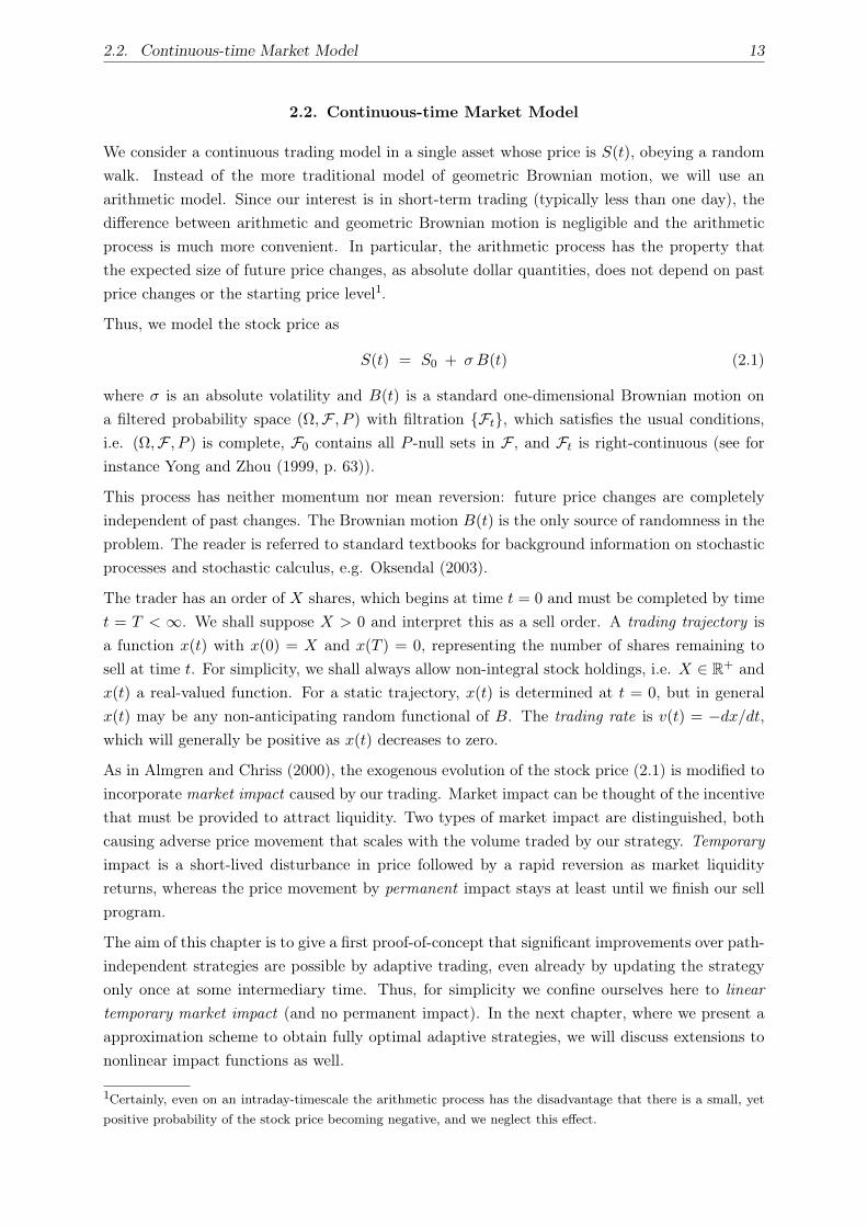
2.2. Continuous-time Market Model
We consider a continuous trading model in a single asset whose price is S(t), obeying a random
walk. Instead of the more traditional model of geometric Brownian motion, we will use an
arithmetic model. Since our interest is in short-term trading (typically less than one day), the
difference between arithmetic and geometric Brownian motion is negligible and the arithmetic
process is much more convenient. In particular, the arithmetic process has the property that
the expected size of future price changes, as absolute dollar quantities, does not depend on past
price changes or the starting price level1.
Thus, we model the stock price as
S(t) = S0 + σ B(t) (2.1)
where σ is an absolute volatility and B(t) is a standard one-dimensional Brownian motion on
a filtered probability space (Ω,F , P ) with filtration Ft, which satisfies the usual conditions,
i.e. (Ω,F , P ) is complete, F0 contains all P -null sets in F , and Ft is right-continuous (see for
instance Yong and Zhou (1999, p. 63)).
This process has neither momentum nor mean reversion: future price changes are completely
independent of past changes. The Brownian motion B(t) is the only source of randomness in the
problem. The reader is referred to standard textbooks for background information on stochastic
processes and stochastic calculus, e.g. Oksendal (2003).
The trader has an order of X shares, which begins at time t = 0 and must be completed by time
t = T < ∞. We shall suppose X > 0 and interpret this as a sell order. A trading trajectory is
a function x(t) with x(0) = X and x(T ) = 0, representing the number of shares remaining to
sell at time t. For simplicity, we shall always allow non-integral stock holdings, i.e. X ∈ R+ and
x(t) a real-valued function. For a static trajectory, x(t) is determined at t = 0, but in general
x(t) may be any non-anticipating random functional of B. The trading rate is v(t) = −dx/dt,
which will generally be positive as x(t) decreases to zero.
As in Almgren and Chriss (2000), the exogenous evolution of the stock price (2.1) is modified to
incorporate market impact caused by our trading. Market impact can be thought of the incentive
that must be provided to attract liquidity. Two types of market impact are distinguished, both
causing adverse price movement that scales with the volume traded by our strategy. Temporary
impact is a short-lived disturbance in price followed by a rapid reversion as market liquidity
returns, whereas the price movement by permanent impact stays at least until we finish our sell
program.
The aim of this chapter is to give a first proof-of-concept that significant improvements over path-
independent strategies are possible by adaptive trading, even already by updating the strategy
only once at some intermediary time. Thus, for simplicity we confine ourselves here to linear
temporary market impact (and no permanent impact). In the next chapter, where we present a
approximation scheme to obtain fully optimal adaptive strategies, we will discuss extensions to
nonlinear impact functions as well.
1Certainly, even on an intraday-timescale the arithmetic process has the disadvantage that there is a small, yet
positive probability of the stock price becoming negative, and we neglect this effect.
14 Chapter 2. Adaptive Trading with Market Impact: Single Update
0 10 20 30 40 50 60 70 80 90 100
9.4
9.6
9.8
10
10.2
10.4
S
0 10 20 30 40 50 60 70 80 90 1000
20
40
60
80
100
x
0 10 20 30 40 50 60 70 80 90 1000
0.5
1
1.5
2
v
t
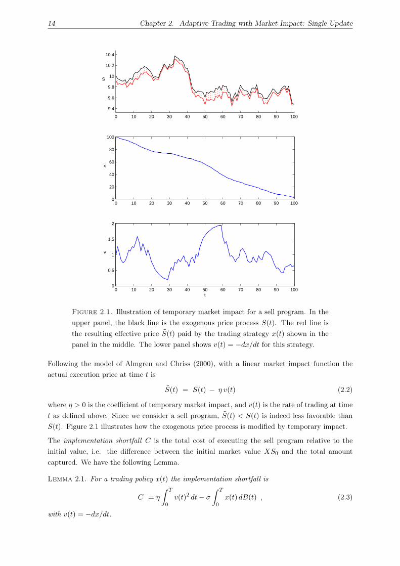
Figure 2.1. Illustration of temporary market impact for a sell program. In the
upper panel, the black line is the exogenous price process S(t). The red line is
the resulting effective price S(t) paid by the trading strategy x(t) shown in the
panel in the middle. The lower panel shows v(t) = −dx/dt for this strategy.
Following the model of Almgren and Chriss (2000), with a linear market impact function the
actual execution price at time t is
S(t) = S(t) − η v(t) (2.2)
where η > 0 is the coefficient of temporary market impact, and v(t) is the rate of trading at time
t as defined above. Since we consider a sell program, S(t) < S(t) is indeed less favorable than
S(t). Figure 2.1 illustrates how the exogenous price process is modified by temporary impact.
The implementation shortfall C is the total cost of executing the sell program relative to the
initial value, i.e. the difference between the initial market value XS0 and the total amount
captured. We have the following Lemma.
Lemma 2.1. For a trading policy x(t) the implementation shortfall is
C = η
∫ T
0v(t)2 dt− σ
∫ T
0x(t) dB(t) , (2.3)
with v(t) = −dx/dt.
2.3. Optimal Path-Independent Trajectories 15
Proof. By the definition of the implementation shortfall C and because of (2.2),
C = X S0 −∫ T
0S(t) v(t) dt
= X S0 −∫ T
0S(t) v(t) dt + η
∫ T
0v(t)2 dt .
Integration by parts for the first integral yields
C = X S0 −[S(t)x(t)
]T0− σ
∫ T
0x(t) dB(t) + η
∫ T
0v(t)2 dt
= η
∫ T
0v(t)2 dt− σ
∫ T
0x(t) dB(t) .
The implementation shortfall C consists of two parts. The first term represents the market
impact cost. The second term represents the trading gains or losses: since we are selling, a
positive price motion gives negative cost.
Note that C is in fact independent of the initial stock price S0, and only depends on the dynamics
of S(t). Hence, optimal trading strategies will also be independent of S0.
As C is a random variable, an “optimal” strategy will seek some risk-reward balance. Almgren
and Chriss (2000) employ the well-known mean-variance framework: a strategy is called efficient
if it minimizes the variance of a specified maximum level of expected cost or conversely.
The set of all efficient strategies is summarized in the efficient frontier of optimal trading, intro-
duced by Almgren and Chriss (2000) in the style of the well-known Markowitz efficient frontier
in portfolio theory.
2.3. Optimal Path-Independent Trajectories
If x(t) is fixed independently of B(t), then C is a Gaussian random variable with mean and
variance
E = η
∫ T
0v(t)2 dt and V = σ2
∫ T
0x(t)2 dt . (2.4)
Using (2.4), Almgren and Chriss (2000) explicitly give the family of efficient static trading tra-
jectories:
Theorem 2.2 (Almgren and Chriss (2000)). The family of efficient path-independent (“static”)
trade trajectories is given by
x(t) = X h(t, T, κ) with h(t, T, κ) =sinh
(κ(T − t)
)
sinh(κT) , (2.5)
parametrized by the static “urgency” parameter κ ≥ 0.
The units of κ are inverse time, and 1/κ is a desired time scale for liquidation, the “half-life” of
Almgren and Chriss (2000). The static trajectory is effectively an exponential exp(−κt) with
adjustments to reach x = 0 at t = T . For fixed κ, the optimal time scale is independent of
portfolio size X since both expected costs and variance scale as X2.

16 Chapter 2. Adaptive Trading with Market Impact: Single Update
Almgren and Chriss determine these efficient trade schedules by optimizing
minx(t)
E + λV (2.6)
for each λ ≥ 0, where E = E [C] and V = Var [C] are the expected value and variance of
C. If restricting to path-independent strategies, the solution of (2.6) is obtained by solving an
optimization problem for the deterministic trade schedule x(t). For given λ ≥ 0, the solution of
(2.6) is (2.5) with κ =√
λσ2/η. By taking κ→ 0, we recover the linear profile x(t) = X(T−t)/T .
This profile has expected cost and variance
Elin = ηX2/T and Vlin = σ2X2T/3 . (2.7)
2.4. Single Update Strategies
We now consider strategies that respond to the stock price movement exactly once, at some
intermediary time T∗ with 0 < T∗ < T . On the first trading period 0 ≤ t ≤ T∗, we follow a static
trading trajectory with initial urgency κ0; that is, the trajectory is x(t) = X h(t, T, κ0) with h
from (2.5). Let X∗(κ0, T∗) = X h(T∗, T, κ0) be the remaining shares at time T∗. At this time,
we switch to a static trading trajectory with one of n new urgencies κ1, . . . , κn: with urgency κi,
we set x(t) = X∗(κ0, T∗)h(t− T∗, T − T∗, κi) for T∗ ≤ t ≤ T . We choose the new urgency based
on the realized cost up until T∗,
C0 = η
∫ T∗
0v(t)2 dt− σ
∫ T∗
0x(t) dB(t) . (2.8)
To that end, we partition the real line into n intervals I1, . . . , In, defined by Ij =bj−1 < C0 <
bj
with bj = E [C0]+aj
√Var [C0] and a1, . . . , an−1 fixed constants (a0 = −∞, an =∞). Then,
on the second period we use κj if C0 ∈ Ij .
Thus, a single-update strategy is defined by the parameters T∗, a1, . . . , an−1 and κ0, . . . , κn. The
overall trajectory is summarized by
x(t) =
Xh(t, T, κ0) for 0 ≤ t ≤ T∗
x(T∗)h(t− T∗, T − T∗, κi) for T∗ < t ≤ T, if C0 ∈ Ii .(2.9)
Note that we do not know which trajectory we shall actually execute in the second period until
we observe C0 at time T∗.
Straightforward calculation shows that h from (2.5) satisfies h(t, T, κ) = h(s, T, κ)h(t−s, T−s, κ)
for 0 ≤ s ≤ t ≤ T . Thus, if we choose κ0 = κ1 = · · · = κn =: κ, the single-update strategy will
degenerate to the static trajectory x(t) = h(t, T, κ). That is, the set of static trajectories from
Theorem 2.2 is indeed a subset of the set of single-update strategies.
Let φ(·) be the standard normal density and Φ(·) its cumulative. We need to prove the following
Lemma about the conditional expectation of a normally distributed random variable.
Lemma 2.3. Let X ∼ N (µ, σ2) and −∞ < a < b <∞. Then
E
[X
∣∣∣∣∣ a ≤X − µ
σ≤ b
]= µ + σ
φ(a)− φ(b)
Φ(b)− Φ(a). (2.10)
2.4. Single Update Strategies 17
Proof. Let Z = X−µσ , i.e. Z ∼ N (0, 1). Recall φ(x) = exp(−x2/2)/
√2π, and hence
∫ b
azφ(z) dz = φ(a)− φ(b) .
We have
E[X 1
a≤X−µσ
≤b
]= µ E [1a≤Z≤b] + σ E [Z 1a≤Z≤b]
= µ P [a ≤ Z ≤ b] + σ
∫ b
azφ(z) dz
= µ(Φ(b)− Φ(a)
)+ σ
(φ(a)− φ(b)
).
Since
E
[X
∣∣∣∣∣ a ≤X − µ
σ≤ b
]· P[a ≤ X − µ
σ≤ b
]= E
[X 1
a≤X−µσ
≤b
],
equation (2.10) follows.
We will now show that single-update strategies can actually significantly improve over path-
independent strategies. The magnitude of the improvement will depend on a single market
parameter, the “market power”
µ =ηX/T
σ√
T. (2.11)
Here the numerator is the price concession for trading at a constant rate, and the denominator
is the typical size of price motion due to volatility over the same period. The ratio µ is a
nondimensional preference-free measure of portfolio size, in terms of its ability to move the
market.
The following Theorem gives mean and variance of a single-update strategy as a function of the
strategy parameters. Below we will use these expressions to determine optimal single-update
strategies, and demonstrate that they indeed improve over the static trajectories of Almgren and
Chriss (2000).
Theorem 2.4. Let µ > 0, and π be a single-update strategy given by the set of parameters
(T∗, a1, . . . , an−1, κ0, κ1, . . . , κn). Then the mean E = E [C] and variance V = Var [C] of π,
scaled by the respective values of the linear strategy (2.7), are given by
E = E/Elin = E0 + E (2.12)
and
V = V/Vlin = V0 + V + 2√
3µ√
V0
n∑
i=1
qiEi + 3µ2n∑
i=1
pi
(Ei − E
)2, (2.13)
18 Chapter 2. Adaptive Trading with Market Impact: Single Update
with pj = Φ(aj)− Φ(aj−1), qj = φ(aj−1)− φ(aj), E =∑n
i=1 piEi, V =∑n
i=1 piVi and
E0 =κ0T
(sinh
(2κ0T
)− sinh
(2κ0(T − T∗)
)+ 2κ0T∗
)
4 sinh2(κ0T ), (2.14)
V0 =3(sinh
(2κ0T
)− sinh
(2κ0(T − T∗)
)− 2κ0T∗
)
4κ0T sinh2(κ0T ), (2.15)
Ei =sinh2
(κ0(T − T∗)
)
sinh2(κi(T − T∗)
) κiT(sinh
(2κi(T − T∗)
)+ 2κi(T − T∗)
)
4 sinh2(κ0T ), (2.16)
Vi =3 sinh2
(κ0(T − T∗)
)
sinh2(κi(T − T∗)
) sinh(2κi(T − T∗)
)− 2κi(T − T∗)
4κiT sinh2(κ0T ). (2.17)
Proof. Recall that C0, defined in (2.8), is the realized cost on the first period. Furthermore,
we denote by Cj (j = 1, . . . , n) the cost incurred on the second part of the trajectory, if urgency
κj is used,
Cj = η
∫ T
T∗v(t)2 dt − σ
∫ T
T∗x(T∗)h(t− T∗, T − T∗, κj) dB(t) . (2.18)
Each variable Ci (i = 0, . . . , n) is Gaussian. By (2.8), (2.18) and the definition of the single-
update strategy (2.9), straightforward integration yields
E [C0] = ηX2
∫ T∗
0−h′(t, T, κ0)
2 dt = E0 · Elin (2.19)
Var [C0] = σ2X2
∫ T∗
0h(t, T, κ0)
2 dt = V0 · Vlin (2.20)
and for i = 1, . . . , n
E [Ci] = ηX∗(κ0, T∗)2
∫ T
T∗−h′(t− T∗, T − T∗, κi)
2 dt = Ei · Elin (2.21)
Var [Ci] = σ2X∗(κ0, T∗)2
∫ T
T∗h(t− T∗, T − T∗, κi)
2 dt = Vi · Vlin (2.22)
(2.23)
where E0, V0, Ei, Vi are defined by (2.14)–(2.17). Elin, Vlin denote the expected cost and variance
of the linear strategy given by (2.7), and X∗(κ0, T∗) = x(T∗) = X h(T∗, T, κ0).
The total cost is
C = C0 + C(C0) (2.24)
where (C0) = i if and only if C0 ∈ Ii.
With the fixed nondimensional quantities
pj = Φ(aj)− Φ(aj−1) and qj = φ(aj−1)− φ(aj) ,
for j = 1, . . . , n, we have P [C0 ∈ Ij ] = pj and by Lemma 2.3,
E[C0
∣∣C0 ∈ Ij
]= E0Elin + (qj/pj)
√V0Vlin .
By linearity of expectation, we readily get E = E [C] = Elin
(E0 + E
)with E =
∑ni=1 piEi.
The variance is more complicated because of the dependence of the two terms in (2.24). We

2.4. Single Update Strategies 19
use the conditional variance formula Var [X] = E [Var [X|Y ]] + Var [E [X|Y ]] to write, with
V =∑n
i=1 piVi,
Var [C] = E[Var
[C0 + C(C0)
∣∣C0
]]+ Var
[E[C0 + C(C0)
∣∣C0
]]
= E[V(C0)Vlin
]+ Var
[C0 + E(C0)Elin
]
= V Vlin + Var [C0] + 2Elin Cov[C0, E(C0)
]+ E2
lin Var[E(C0)
].
By definition, Var [C0] = V0Vlin, and Var[E(C0)
]=∑n
i=1 pi
(Ei − E
)2. Also,
Cov[C0, E(C0)
]= E
[C0 E(C0)
]− E [C0] E
[E(C0)
]
=n∑
i=1
P [C0 ∈ Ii] E[C0E(C0)
∣∣C0 ∈ Ii
]− E [C0] E
[E(C0)
]
=n∑
i=1
piEiElin E[C0
∣∣C0 ∈ Ii
]− E [C0] E
[E(C0)
]
=n∑
i=1
piEiElinE0Elin +n∑
i=1
qiEiElin
√V0Vlin − E [C0] E
[E(C0)
]
= E [C0]n∑
i=1
piEiElin +√
V0VlinElin
n∑
i=1
qiEi − E [C0] E[E(C0)
]
=√
V0VlinElin
n∑
i=1
qiEi .
Putting all this together, we have
V = Var [C] = V0Vlin + V Vlin + 2√
V0VlinElin
n∑
i=1
qiEi + E2lin
n∑
i=1
pi
(Ei − E
)2.
Since E2lin/Vlin = 3µ2 and
√VlinElin/Vlin =
√3µ, (2.13) follows.
As can be seen, scaling expectation and variance of the total cost C by their respective values of
the linear strategy yields expressions E/Elin and V/Vlin as functions of the strategy parameters
ai, κi, and the single market parameter µ. That is, we reduce the four dimensional parameters
X, T, σ and η to one nondimensional (i.e. scalar) parameter, the market power µ.
2.4.1. Density of Total Cost C for Single-update Strategies. In the following, to shorten
notation we denote Ei = E [Ci] = Ei · Elin and Vi = Var [Ci] = Vi · Vlin (i = 0 . . . n) defined
by (2.19, 2.20, 2.21, 2.22). Each Ci is Gaussian with mean Ei and variance Vi, so its density
is fi(ci) = 1/√
2πVi exp(−(Ci − Ei)
2/2Vi
). Let f(c) be the density of the total cost C =
C0 + C(C0), see (2.24). That is, the total cost C is a certain mixture of Gaussians. We have
f(c) =n∑
i=1
∫
Ii
f0(c0) fi(c− c0) dc0
=n∑
i=1
1
2π√
V0Vi
∫ bi
bi−1
exp
(−(c0 − E0)
2
2V0
− (c− c0 − Ei)2
2Vi
)dc0 ,
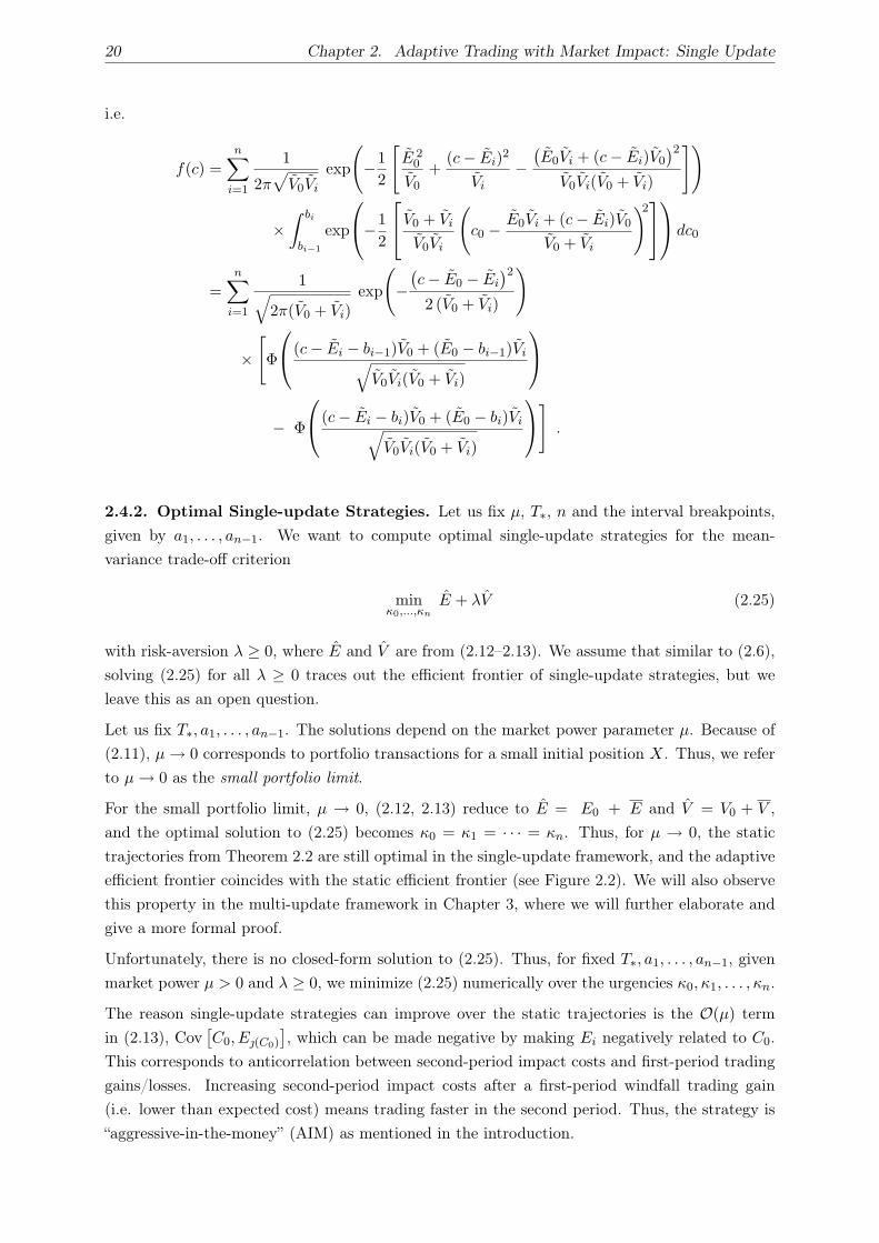
20 Chapter 2. Adaptive Trading with Market Impact: Single Update
i.e.
f(c) =
n∑
i=1
1
2π√
V0Vi
exp
(−1
2
[E 2
0
V0
+(c− Ei)
2
Vi
−(E0Vi + (c− Ei)V0
)2
V0Vi(V0 + Vi)
])
×∫ bi
bi−1
exp
−1
2
V0 + Vi
V0Vi
(c0 −
E0Vi + (c− Ei)V0
V0 + Vi
)2 dc0
=n∑
i=1
1√2π(V0 + Vi)
exp
(−(c− E0 − Ei
)2
2 (V0 + Vi)
)
×[Φ
(c− Ei − bi−1)V0 + (E0 − bi−1)Vi√
V0Vi(V0 + Vi)
− Φ
(c− Ei − bi)V0 + (E0 − bi)Vi√
V0Vi(V0 + Vi)
]
.
2.4.2. Optimal Single-update Strategies. Let us fix µ, T∗, n and the interval breakpoints,
given by a1, . . . , an−1. We want to compute optimal single-update strategies for the mean-
variance trade-off criterion
minκ0,...,κn
E + λV (2.25)
with risk-aversion λ ≥ 0, where E and V are from (2.12–2.13). We assume that similar to (2.6),
solving (2.25) for all λ ≥ 0 traces out the efficient frontier of single-update strategies, but we
leave this as an open question.
Let us fix T∗, a1, . . . , an−1. The solutions depend on the market power parameter µ. Because of
(2.11), µ→ 0 corresponds to portfolio transactions for a small initial position X. Thus, we refer
to µ→ 0 as the small portfolio limit.
For the small portfolio limit, µ → 0, (2.12, 2.13) reduce to E = E0 + E and V = V0 + V ,
and the optimal solution to (2.25) becomes κ0 = κ1 = · · · = κn. Thus, for µ → 0, the static
trajectories from Theorem 2.2 are still optimal in the single-update framework, and the adaptive
efficient frontier coincides with the static efficient frontier (see Figure 2.2). We will also observe
this property in the multi-update framework in Chapter 3, where we will further elaborate and
give a more formal proof.
Unfortunately, there is no closed-form solution to (2.25). Thus, for fixed T∗, a1, . . . , an−1, given
market power µ > 0 and λ ≥ 0, we minimize (2.25) numerically over the urgencies κ0, κ1, . . . , κn.
The reason single-update strategies can improve over the static trajectories is the O(µ) term
in (2.13), Cov[C0, E(C0)
], which can be made negative by making Ei negatively related to C0.
This corresponds to anticorrelation between second-period impact costs and first-period trading
gains/losses. Increasing second-period impact costs after a first-period windfall trading gain
(i.e. lower than expected cost) means trading faster in the second period. Thus, the strategy is
“aggressive-in-the-money” (AIM) as mentioned in the introduction.
2.6. Conclusion 21
2.5. Numerical Results
In Figure 2.2 we plot E and V relative to Elin and Vlin; each curve is computed by varying
λ in (2.25) from 0 to ∞, for a fixed value of µ. The solution for each pair (λ, µ) is computed
using n = 2, and a1 = 0 (a0 = −∞, a2 = ∞). That is, we consider single-update strategies
which switch to one of two trajectories, depending on whether the realized cost in the first part
was higher or lower than its expected value. We fix T∗ to the half-life of the corresponding
static trajectory. The plot also shows the frontier corresponding to the static trajectories from
Theorem 2.2 (solid curve). As can be seen, this frontier indeed corresponds to the limit µ→ 0.
We use these frontiers to obtain cost distributions for adaptive strategies that are better than
the cost distributions for any static strategy. In Figure 2.2, the point marked on the static
frontier (solid curve) corresponds to a static trajectory computed with parameter κ = 14, giving
a Gaussian cost distribution. For a portfolio with µ = 0.15, this distribution has expectation
E ≈ 7.0 × Elin and variance V ≈ 0.11 × Vlin. The inset shows this distribution as a black
dashed line. The inset also shows the cost distributions associated with the adaptive strategies
corresponding to the two marks on the frontier for µ = 0.15 (outermost dashed curve): one
of them has the same mean, but lower variance (V ≈ 0.06 × Vlin); the other one has same
variance, but lower mean (E ≈ 4.47 × Elin). These distributions are the extreme points of
a one-parameter family of distributions along the adaptive frontier, each of which is strictly
preferable to the given static strategy for a mean-variance investor. The distribution plots of
the adaptive strategies are generated from the density formula derived in Section 2.4.1. These
cost distributions are slightly skewed toward positive costs. But as they are not too far from
Gaussian, we can still expect mean-variance to gives reasonable results (Recall that for Gaussian
random variables, mean-variance optimization is consistent with expected utility maximization
and stochastic dominance; see for instance Levy (1992); Bertsimas et al. (2004)).
Figure 2.3 shows an example of a single-update trading strategy for µ = 0.15. The dashed
line is the static optimal trajectory with urgency κ = 14. We choose the efficient adaptive
strategy, which achieves the same variance as this static trajectory, but has lower expected cost.
The adaptive strategy initially trades more slowly than the optimal static trajectory. At T∗, if
prices have moved in the trader’s favor and the realized cost is lower than the expected value
(conditional on t = 0), then the strategy accelerates, spending the investment gains on impact
costs. If prices have moved against the trader, corresponding to higher than expected values
of C0, then the strategy decelerates to save impact costs in the remaining period. Thus, the
single-update strategy is indeed “aggressive-in-the money” (AIM).
2.6. Conclusion
The single-update strategies presented in this chapter demonstrate that price adaptive scaling
strategies can lead to significant improvements over static trade schedules (Almgren and Chriss,
2000) for the execution of portfolio transactions, and they illustrate the importance of the new
“market power” parameter µ. Unfortunately, the single-update framework presented in this
chapter does not directly generalize to multi-decision frameworks.
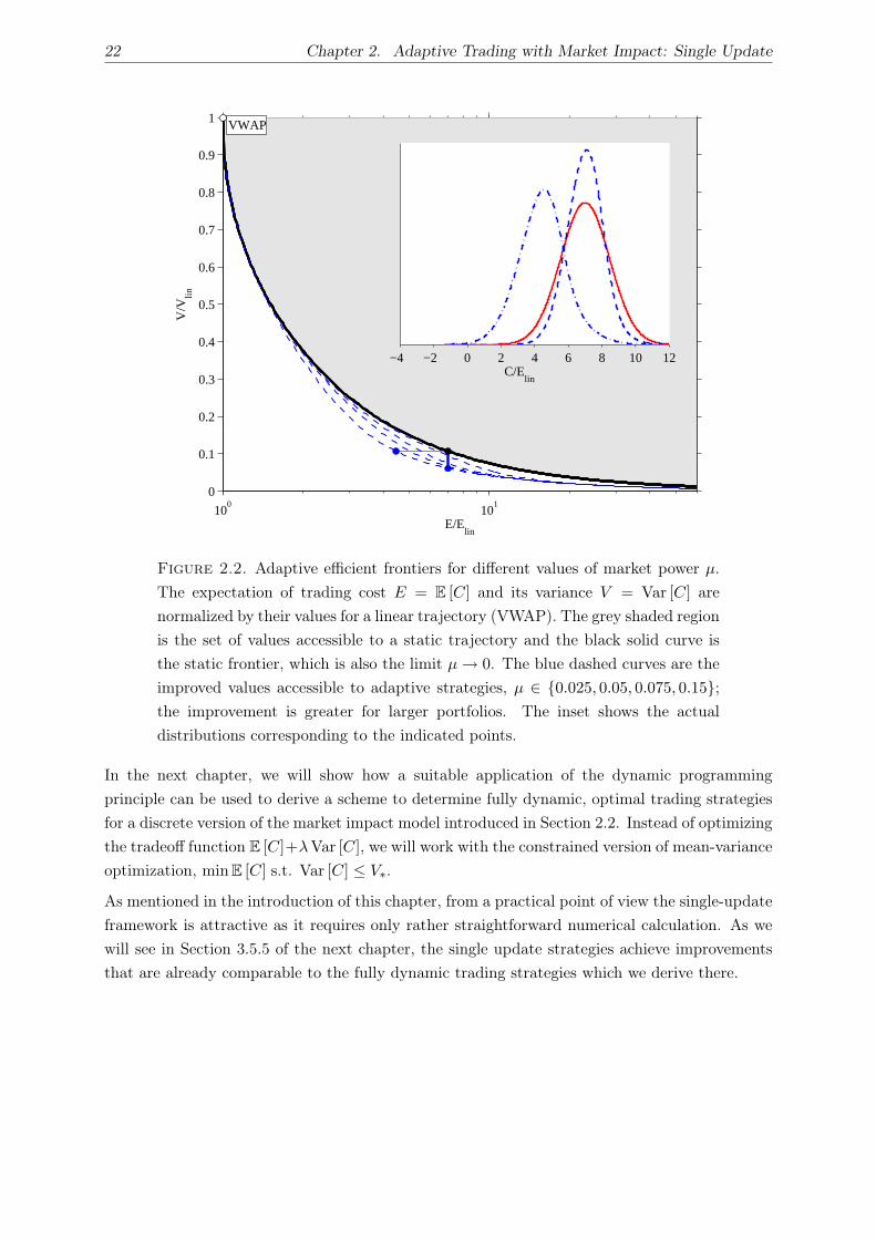
22 Chapter 2. Adaptive Trading with Market Impact: Single Update
100
101
0
0.1
0.2
0.3
0.4
0.5
0.6
0.7
0.8
0.9
1 VWAP
E/Elin
V/V
lin
−4 −2 0 2 4 6 8 10 12C/E
lin
Figure 2.2. Adaptive efficient frontiers for different values of market power µ.
The expectation of trading cost E = E [C] and its variance V = Var [C] are
normalized by their values for a linear trajectory (VWAP). The grey shaded region
is the set of values accessible to a static trajectory and the black solid curve is
the static frontier, which is also the limit µ→ 0. The blue dashed curves are the
improved values accessible to adaptive strategies, µ ∈ 0.025, 0.05, 0.075, 0.15;the improvement is greater for larger portfolios. The inset shows the actual
distributions corresponding to the indicated points.
In the next chapter, we will show how a suitable application of the dynamic programming
principle can be used to derive a scheme to determine fully dynamic, optimal trading strategies
for a discrete version of the market impact model introduced in Section 2.2. Instead of optimizing
the tradeoff function E [C]+λ Var [C], we will work with the constrained version of mean-variance
optimization, min E [C] s.t. Var [C] ≤ V∗.
As mentioned in the introduction of this chapter, from a practical point of view the single-update
framework is attractive as it requires only rather straightforward numerical calculation. As we
will see in Section 3.5.5 of the next chapter, the single update strategies achieve improvements
that are already comparable to the fully dynamic trading strategies which we derive there.

2.6. Conclusion 23
0 0.1 0.2 0.3 0.4 0.5 0.6 0.7 0.8 0.9 10
0.1
0.2
0.3
0.4
0.5
0.6
0.7
0.8
0.9
1
Time t
Sha
res
rem
aini
ng x
(t)
0.000
5
10
15
20
Normalized cost C0
Urgency κ
Figure 2.3. Example of an adaptive trading trajectories for market power µ =
0.15. The dashed line is a static optimal trajectory with urgency κ = 14; the
adaptive strategy with n = 2 and a1 = 0 is chosen such that it achieves the same
variance as this static trajectory, but lower expected cost. The inset shows the
dependence of the new urgency on the initial trading cost C0, normalized by the
ex ante expectation and standard deviation of C0.

CHAPTER 3
Optimal Adaptive Trading with Market Impact
In this chapter we further discuss the optimal dynamic execution of portfolio transactions in
the market impact model of Almgren and Chriss (2000). Improving over the single update
strategies presented in the previous chapter, in this chapter we show how a suitable application
of the dynamic programming principle can be used to derive a scheme to determine fully optimal
dynamic trading strategies for the execution problem in discrete time. Our adaptive strategies
significantly improve over the static arrival price algorithms of Almgren and Chriss (2000) with
respect to the mean-variance trade-off evaluated at the initial time.
3.1. Introduction
In this chapter we further study adaptive trading strategies for the market impact model intro-
duced in Section 1.2 with the implementation shortfall as benchmark, i.e. the difference between
the average execution price and the pre-trade price. In the previous chapter we showed that
adaptive trading strategies can indeed significantly improve over the arrival price algorithms of
Almgren and Chriss (2000) with respect to the mean-variance trade-off evaluated at the ini-
tial time. However, the single-update strategies considered there do not generalize to multiple
updates or fully optimal adaptive trading.
As mentioned in Section 1.2, a related problem is mean-variance portfolio optimization in a
multiperiod setting: executing a buy order can be seen as an optimal portfolio strategy in one
risky asset (the stock to be purchased) and one riskless asset (cash) under transaction costs and
with the additional terminal constraint that the entire wealth is in the stock at the end of the
buy progam at t = T . Only recently Li and Ng (2000) gave a closed-form solution for the mean-
variance problem in a discrete-time multiperiod setting. They use an embedding technique of the
original problem into a family of tractable auxiliary problems with a utility function of quadratic
type. While in principle this approach may be applied to the portfolio transaction problem as
well, the market impact terms together with the need to introduce a second parameter in the
auxiliary problem (next to the risk aversion) significantly complicate the problem.
We therefore follow a different approach to determine optimal trading strategies with respect to
the specification of measuring risk and reward at the initial time. Using a dynamic program-
ming principle for mean-variance optimization, we determine fully optimal Markovian trading
strategies for the arrival price problem in a discrete time setting. The key idea is to use the
variance of total cost as the value function, and consider the targeted expected return as a state
variable. We give an efficient scheme to obtain numerical solutions by solving a series of convex
constrained optimization problems.
25

26 Chapter 3. Optimal Adaptive Trading with Market Impact
We observe the same qualitative behavior as in the previous chapter. First, the improvement
through adaptivity is larger for large transactions, expressed in terms of the market power
µ, (2.11); for small portfolios, µ → 0, optimal adaptive trade schedules coincide with opti-
mal static trade schedules. Second, the improvement through a dynamic strategy comes from
introducing a correlation between the trading gains or losses and market impact costs incurred
in the remainder. If the price moves in the trader’s favor in the early part of the trading, then
the algorithm spends parts of those gains on market impact costs by accelerating the remainder
of the program. If the price moves against the trader, then the algorithm reduces future market
impact costs by trading more slowly. Thus, our new optimal trade schedules are “aggressive-in-
the-money” (AIM). A “passive-in-the-money” (PIM) strategy would react oppositely (Kissell and
Malamut, 2005).
One important reason for using a AIM or PIM strategy would be the expectation of serial
correlation in the price process. Our strategies arise in a pure random walk model with no serial
correlation, using pure classic mean and variance. This provides an important caveat for our
formulation. Our strategy suggests to “cut your gains and let your losses run.” If the price
process does have any significant momentum, then this strategy can cause much more serious
losses than the gains it provides. Thus we do not advocate implementing them in practice before
doing extensive empirical tests.
The remainder of this chapter is organized as follows: In Section 3.2 we present the market and
trading model. In contrast to Chapter 2, we consider a discrete time setting. In Section 3.3 we
review the concept of mean variance efficient strategies in discrete time, the efficient frontier of
trading as well as the optimal static trajectories of Almgren and Chriss (2000). In Section 3.4,
we show how to construct fully optimal adaptive policies by means of a dynamic programming
principle for mean-variance optimization. In Section 3.5 we give numerical results.
3.2. Trading Model
Let us start by reviewing the discrete trading model considered by Almgren and Chriss (2000).
We confine ourselves to sell programs in a single security. The definitions and results for a buy
program are completely analogous. Furthermore, an extension to multiple securities (“basket
trading”) is possible.
Suppose we hold a block of X shares of a stock that we want to completely sell by time T .
We divide the trading horizon T into N intervals of length τ = T/N , and define discrete times
tk = kτ , k = 0, . . . , N . A trade schedule π is a list of stock holdings (x0, x1, . . . , xN ) where xk
is the number of shares we plan to hold at time tk; we require x0 = X and xN = 0. Thus we
shall sell x0 − x1 shares between t0 and t1, x1 − x2 shares between times t1 and t2 and so on.
We require a pure sell program which may never buy shares, that is x0 ≥ x1 ≥ · · · ≥ xN . Our
strategy comprises N sales, and effectively N − 1 decision variables x1, . . . , xN−1. The average
rate of trading during the time interval tk−1 to tk is vk = (xk−1 − xk)/τ . Crucially, this trade
list need not be fixed in advance but may depend on the observed price evolution: π must be
adapted to the filtration of the price process as described below.

3.2. Trading Model 27
The stock price follows a random walk, modified to incorporate permanent and temporary impact
due to our trading. Temporary impact is a short-lived disturbance in price followed by a rapid
reversion as market liquidity returns, whereas the price movement by permanent impact stays at
least until we finish our sell program. As in Chapter 2, we employ an arithmetic model for the
stock price. For the intraday time scales of interest to us, the difference between an arithmetic
and a geometric model is negligible, and an arithmetic model is much simpler mathematically.
Thus, we take the price to follow the process
Sk = Sk−1 + στ1/2ξk − τg(xk−1 − xk
τ
), (3.1)
for k = 1, . . . , N . Here ξk are independent random variables on Ω with an arbitrary distribution,
having E [ξk] = 0 and Var [ξk] = 1. Unless stated otherwise, we shall always assume that Ω is
finite, |Ω| < ∞. For example, for a binomial tree model we would set Ω = ±1. g(v) is a
permanent impact function and will be described below.
Let Fk be the σ-algebra generated by ξ1, . . . , ξk, for k = 0, . . . , N . For k = 0, . . . , N − 1, Fk−1
is the information available to the investor before he makes his decision xk, 1 ≤ k ≤ N − 1,
i.e. xk must be Fk−1 measurable. That is, we allow each trade decision xk to depend on prices
S0, . . . , Sk−1 but not on Sk or ξk; the strategy π is adapted to the filtration of the price motion.
Thus the first trade decision x0−x1 must be nonrandom; the second decision x1−x2 may depend
on the realization of the first price increment ξ1, etc.
σ is the absolute volatility of the stock per unit time, so σ2τ is the variance of price change over
a single time step, and the variance of price change over the entire trading period is σ2T . The
permanent impact g(v) is a measurable, convex and continuous function of the average rate of
trading v = (xk−1 − xk)/τ ≥ 0 during the interval tk−1 to tk, with g(v) ≥ 0 for all v ≥ 0.
Temporary market impact is modeled by considering our trade price to be slightly less favorable
than the “market” price Sk. Hence, the effective price per share when selling xk−1 − xk during
the interval tk−1 to tk is
Sk = Sk−1 − h(xk−1 − xk
τ
), (3.2)
for some measurable, continuous function h(v) ≥ 0 for all v ≥ 0. We shall require that v h(v) is
convex. Unlike permanent impact g(v), the temporary impact effect h(v) does not affect the next
market price Sk. Figure 3.1 illustrates how the exogenous price process is modified by temporary
market impact.
For a sell program π = (x0, x1, . . . , xN ), the capture upon completion is
N∑
k=1
(xk−1 − xk) Sk = XS0 + στ1/2N∑
k=1
ξkxk
− τN∑
k=1
xk g(xk−1 − xk
τ
)−
N∑
k=1
(xk−1 − xk)h(xk−1 − xk
τ
).
The first term on the right side is the initial market value of the position. The second term
represents trading gains or losses due to volatility; note that this term has strictly zero expected
value for any adapted strategy. The third and fourth terms are the losses due to permanent and
temporary impact.
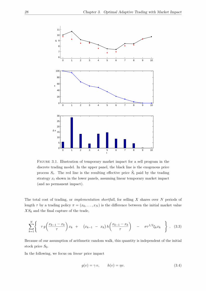
28 Chapter 3. Optimal Adaptive Trading with Market Impact
0 1 2 3 4 5 6 7 8 9 106
7
8
9
10
11
S
0 1 2 3 4 5 6 7 8 9 100
5
10
15
20
25
30
∆ x
t
0 1 2 3 4 5 6 7 8 9 100
20
40
60
80
100
x
Figure 3.1. Illustration of temporary market impact for a sell program in the
discrete trading model. In the upper panel, the black line is the exogenous price
process St. The red line is the resulting effective price St paid by the trading
strategy xt shown in the lower panels, assuming linear temporary market impact
(and no permanent impact).
The total cost of trading, or implementation shortfall, for selling X shares over N periods of
length τ by a trading policy π = (x0, . . . , xN ) is the difference between the initial market value
XS0 and the final capture of the trade,
N∑
k=1
τ g
(xk−1 − xk
τ
)xk +
(xk−1 − xk
)h
(xk−1 − xk
τ
)− στ1/2ξkxk
. (3.3)
Because of our assumption of arithmetic random walk, this quantity is independent of the initial
stock price S0.
In the following, we focus on linear price impact
g(v) = γ v, h(v) = ηv. (3.4)

3.3. Efficient Frontier of Optimal Execution 29
Then, as noted by Almgren and Chriss (2000) it suffices to consider temporary impact only,
because with the linear impact functions (3.4) the expression for the cost (3.3) is
N∑
k=1
γ(xk−1 − xk)xk +
η
τ(xk−1 − xk)
2 − στ1/2ξkxk
. (3.5)
Since
1
2X2 =
1
2
( N∑
k=1
(xk−1 − xk))2
=N∑
k=1
(xk−1 − xk)xk +1
2
N∑
k=1
(xk−1 − xk)2 ,
(3.5) becomes
1
2γX2 +
N∑
k=1
−1
2γ(xk−1 − xk)
2 +η
τ(xk−1 − xk)
2 − στ1/2ξkxk
=1
2γX2 +
N∑
k=1
η
τ(xk−1 − xk)
2 − στ1/2ξkxk
with η = η − 12γτ . Neglecting the constant γX2/2 and replacing η ← η (implicitly assuming
that τ is small enough that η > 0), we obtain
C(X, N, π) =η
τ
N∑
k=1
(xk−1 − xk)2 − στ1/2
N∑
k=1
ξkxk , (3.6)
In the remainder of this chapter, we shall always work with (3.6) as the expression for the cost
of a N period strategy π to sell X shares.
We assume that volatility, as well as the dependence of permanent impact and on our trade de-
cisions, are not only non-random and known in advance but have a uniform profile. Predictable
intraday seasonality can largely be handled by interpreting time t as a “volume time” correspond-
ing to the market’s average rate of trading. Random variations in volatility and liquidity are
more difficult to model properly (Walia, 2006).
As τ → 0, that is as N →∞ with T fixed, this discrete trading model converges to a continuous
process: the exogenous price process is an arithmetic Brownian motion, the shares process is an
adapted function x(t), and the instantaneous trade rate is v(t) = −dx/dt. Hence, the scheme
that we will give in the rest of this chapter to determine optimal strategies immediately yields a
scheme to determine optimal strategies also for the arrival price problem in a continuous setting
as introduced in Chapter 2. The same techniques would also work with nonlinear cost functions,
with a drift term added to the price dynamics, or for multi-asset portfolios.
3.3. Efficient Frontier of Optimal Execution
For any trading strategy, the final implementation shortfall C(X, N, π) is a random variable:
not only do the price motions ξk directly affect our trading gains or losses, but for an adapted
strategy the trade list itself may be different on each realization, according to the rule π. An
“optimal” strategy will determine some balance between minimizing the expected cost and its
variance.

30 Chapter 3. Optimal Adaptive Trading with Market Impact
Let
D(X, N) =
(π, C
)
∣∣∣∣∣∣∣∣
π = (x0, x1, . . . , xN ) with x0 = X, xN = 0
x0 ≥ x1 ≥ · · · ≥ xN
C(X, N, π) ≤ C a.e.
(3.7)
be the set of all adapted trading policies that sell X shares in N periods. We require a pure
sell program, x0 ≥ x1 ≥ · · · ≥ xN , that is the strategy may never buy shares. π is the trade
schedule and must be adapted to the filtration Fk of the stock price process Sk as described
above. C is the cost strategy, which is a FN -measurable random variable that gives the trading
cost associated with this policy for each path of the (random) stock price process. For each path
of the stock price process, C must be at least the cost (3.6) of the execution strategy π, but the
specification “C(X, N, π) ≤ C” allows the trader to deliberately incur extra costs if that improves
his trade-off. Since C and C(X, N, π) are random variables that give a cost for each realization
of the stock price process, C > C(X, N, π) means that the trader may selectively account more
than the actual cost (3.6) in some realizations of the stock price. We will discuss this issue in
Section 3.4.3.
For given E ∈ R, let
A (X, N, E) =
(π, C) ∈ D(X, N)∣∣∣ E
[C]≤ E
(3.8)
be the subset of policies for which the expected cost is at most E (as described below, this set
can be empty if E is too small).
Mean-variance optimization solves the constrained problem
For E ∈ R, minimize Var[
C]
over (π, C) ∈ A (X, N, E) . (3.9)
The solutions are efficient trading strategies such that no other strategy has lower variance for
the same level (or lower) of expected costs. By varying E ∈ R we determine the family of all
efficient strategies
E (X, N) =
(π, C) ∈ D(X, N)∣∣∣ ∄ (π, C) ∈ D(X, N) s.t.
(E[ C ] ≤ E
[C]∧ Var
[C]
< Var[
C] )
. (3.10)
Plotting Var[C]
vs E[C]
for all (π, C) ∈ E (X, N), we obtain a downward-sloping curve in the
V -E plane, the efficient frontier of optimal trading strategies (Almgren and Chriss, 2000). The
set of efficient strategies E (X, N) is independent of the initial stock price S0. This is by virtue
of the arithmetic random walk (3.1).
The feasible domain A (X, N, E) of (3.9) is empty if the target expected cost E is too small. To
determine the minimum possible expected cost, note that the last term in (3.6) has strictly zero
expected value. Minimizing the remaining term E[∑
(xk−1 − xk)2]
gives the nonrandom linear
strategy πlin with xk−1 − xk = X/N for k = 1 . . . N , and C = C(X, N, πlin). The expectation
and variance of total cost of this strategy are
Elin(X, N) =ηX2
Nτ=
ηX2
T, (3.11)
Vlin(X, N) =1
3σ2X2 Nτ
(1− 1
N
)(1− 1
2N
). (3.12)
3.3. Efficient Frontier of Optimal Execution 31
Since Nτ = T is the fixed trading duration, Elin is independent of the discretization parameter N ,
and Vlin depends only weakly on N when N is large. In volume time, this strategy is equivalent
to the popular VWAP profile (see for instance Madhavan (2002)).
The other extreme is to sell the entire position in the first time period: πinst with x1 = · · · =xN = 0. This yields Vinst(X, N) = 0 and an expectation of
Einst(X) =ηX2
τ. (3.13)
We have Elin ≥ Einst, and in fact C = C(X, N, πinst) = Einst(X) is non-random. For τ → 0,
Einst(X) becomes arbitrarily large.
From this discussion, we conclude that A (X, N, E) is non-empty exactly if Elin(X, N) ≤ E.
For Elin, the mean and variance are both proportional to the square of the initial position X.
This is a general feature of linear impact functions, since the impact per share is linear in the
trade size, and the total dollar cost is the per-share cost multiplied by the number of shares; the
variance is always quadratic in the number of shares.
3.3.1. Static Trajectories. We distinguish two types of trading strategies: path-independent
and path-dependent. Path-independent strategies are determined in advance of trading at time
t0, and are deterministic schedules that depend only on information available at time t0. Path-
dependent strategies, conversely, are arbitrary non-anticipating trading policies for which each
xk depends on all information up to and including time tk. In the following, we shall refer to
path-independent strategies as static strategies, and to path-dependent strategies as adaptive or
dynamic.
More precisely, for a static trading strategy we require π = (x0, . . . , xN ) to be fixed at the start of
trading, independently of the ξk, and C = C(X, N, π). Then C(X, N, π) has mean and variance
E [C(X, N, π)] =η
τ
N∑
k=1
(xk−1 − xk)2, Var [C(X, N, π)] = σ2τ
N∑
k=1
x2k ,
and (3.9) becomes
minx1≥···≥xk−1
σ2τ
N∑
k=1
x2k
∣∣∣∣∣η
τ
N∑
k=1
(xk−1 − xk)2 ≤ E
(3.14)
with x0 = X and xN = 0. As in the continuous time case in Theorem 2.2 in Chapter 2, the
solutions are given by the family
xj = Xsinh(κ(T − tj))
sinh(κT ), j = 0, . . . , N , (3.15)
with the urgency parameter κ. For given E ≥ 0, the explicit solution of (3.14) is then obtained
by substituting (3.15) into (3.14) and solving for κ.
The execution strategy is independent of the portfolio size X except for an overall factor, and
the expected value and variance of total cost are quadratic in portfolio size. This is an artifact
of the linear impact model; for nonlinear models the trajectories do depend on portfolio size and
the cost does not have a simple expression (Almgren, 2003).
32 Chapter 3. Optimal Adaptive Trading with Market Impact
3.4. Optimal Adaptive Strategies
As seen in the previous section, we can construct optimal static trading strategies by solving a
straightforward optimization problem. On the other hand, determining optimal adaptive strate-
gies is a difficult problem. In the previous chapter, we demonstrated that adaptive strategies
can improve over static trajectories – even adaptive trade schedules which update only once
at an intermediate time T ∗ and follow path-independent trade schedules before and after that
“intervention” time. As we discussed there, this approach does not generalize to fully optimal
adaptive strategies. We will now present a dynamic programming technique to determine optimal
dynamic strategies to any degree of precision.
3.4.1. Dynamic programming. It is alluring to use dynamic programming (Bellman, 1957) to
determine optimal trading strategies for the mean-variance criterion E [Y ] + λ Var [Y ], since this
technique works so well for objective functions of the form E [u(Y )]. But dynamic programming
for expected values relies on the “smoothing property” E [E [u(Y )|X]] = E [u(Y )]. For the square
of the expectation in the variance term Var [Y ] = E[Y 2]− E [Y ]2, there is no analog of this
expression, and it is difficult to see how to design an iterative solution procedure.
However, with a suitable choice of the value function, mean-variance optimization is indeed
amenable to dynamic programming. The dynamic programming principle for mean-variance
relies on the following counterpart to the smoothing property of expectation, known as the law
of total variance.
Lemma 3.1. Let X and Y be random variables on the same probability space, and Var [Y ] <∞.
Then
Var [Y ] = Var [ E [Y |X]] + E [ Var [Y |X]] .
Proof. Follows from
Var [E [Y |X]] = E[E [Y |X]2
]− E [E [Y |X]]2 = E
[E [Y |X]2
]− E [Y ]2
and
E [Var [Y |X]] = E[E[Y 2|X
]]− E
[E [Y |X]2
]= E
[Y 2]− E
[E [Y |X]2
].
For (π, C) ∈ D(X, N) (with N ≥ 2), π = (X, x1, . . . , xN−1, 0), denote
(π, C)ξ1=a1 the “tail” of the trading strategy (π, C)
for the remaining N − 1 trading periods conditional on the outcome ξ1 = a1 of the first period.
This tail strategy has the trade schedule
πξ1=a1 = (x1, . . . , xN−1, 0) ∈ D(x1, N − 1) ,
and the cost random variable Cξ1=a1 . That is, the cost C of the total strategy in terms of the
cost strategies of its tails is
C = Cξ1 +η
τ(x− x1)
2 − στ1/2ξ1x1 . (3.16)
Note that an adaptive policy (π, C) may use the information ξ1 = a1 from time t1 onwards,
hence in general (π, C)ξ1=a1 indeed depends on the realization a1.
3.4. Optimal Adaptive Strategies 33
The key ingredient in dynamic programming is to write the time-dependent optimization problem
on N periods as the combination of a single-step optimization with an optimization on the
remaining N − 1 periods. We must carefully define the parameters of the (N − 1)-step problem
so that it gives the same solution as the “tail” of the N -step problem.
In Almgren and Chriss (2000), the risk-aversion parameter λ is constant in time and is constant
across realizations of the price process ξ1 ∈ Ω. For the expected utility function, Schied and
Schöneborn (2007) hold constant the analogous parameter α. For our mean-variance formulation,
the following Lemma asserts that the “tail” of the initial strategy is indeed an optimal strategy
across N − 1 steps, if it is defined to be the minimum-variance solution for an appropriate cost
limit E [C]. This cost limit is taken to be the expected value of the remainder of the initial
strategy, and will be different in each realization.
Lemma 3.2. For N ≥ 2, let (π, C) ∈ E (X, N) be an efficient policy, π = (X, x1, . . . , xN−1, 0),
for (3.9). Then
(π, C)ξ1=a ∈ E (x1, N − 1) for almost all outcomes a ∈ Ω of ξ1 ,
that is, B = a ∈ Ω | (π, C)ξ1=a /∈ E (x1, N − 1) has probability zero.
Proof. For each a ∈ B (if B is empty the result is immediate), the tail-strategy (π, C)ξ1=a is
not efficient, and thus there exists (π∗a, C
∗a) ∈ D
(x1, N − 1
)such that
E[
C∗a
]= E
[Cξ1=a
]∧ Var
[C
∗a
]< Var
[Cξ1=a
].
Define (π, C) by replacing the policy for t1 to tN in (π, C) by (π∗a, C
∗a) for all a ∈ B if ξ1 = a
(and identical to π for all other outcomes Ω \B of ξ1). Then by definition
C ≥ C(X, N, π) a.e. (3.17)
and hence (π, C) ∈ D(X, N). Also by construction, we have
E[ C ] = E[
C]
,
and conditional on ξ1 ∈ B
Var[ C | ξ1] < Var[C | ξ1
].
If B has positive probability then1
E[Var[C | ξ1 ∈ B]
]< E
[Var
[C | ξ1 ∈ B
]]
and hence, by the law of total variance,
Var[C] = Var[E[C | ξ1]] + E[Var[C | ξ1]] < Var[E[C | ξ1
]]+ E
[Var[C | ξ1]
]= Var
[C]
,
contradicting (π, C) ∈ E (X, N).
1In general, let (Ω,A, µ) be a measure space and f a measurable function with f > 0 a.e. ThenZ
B
fdµ > 0 for all measurable sets B with µ(B) > 0 . (3.18)
This follows from the Theorem of Beppo-Levi, which asserts that
supn∈N
Z
Ω
fndµ =
Z
Ω
supn∈N
fndµ
for every monotone increasing sequence of non-negative functions. For (3.18), we set Bn = B ∩ x | f(x) ≥ 1/n,and define fn(x) = x for x ∈ Bn and fn(x) = 0 otherwise.

34 Chapter 3. Optimal Adaptive Trading with Market Impact
Lemma 3.2 shows a Markov property of mean-variance efficient strategies, and constitutes the
foundation of why the dynamic programming principle is applicable. Dynamic programming can
be used for all types of risk-measurement which satisfy such a Markov property. For instance, it
naturally holds for the optimization of the expected utilty of a final payoff (see also Appendix A).
Unfortunately, most other risk measures don’t satisfy this property (see Artzner et al. (2007)).
For k ≥ 1 and for fixed τ , we define the value function
Jk(x, c) = min(π,C)∈A (x,k,c)
Var[C]
(3.19)
for x ≥ 0 (we will always assume a non-negative number of shares left to sell since we consider pure
sell programs which are not allowed to buy shares). Note that for |Ω| <∞, the space A (x, k, c)
is finite-dimensional and minimizing solutions will exist; we leave this issue for |Ω| = ∞ as an
open question.
If the cost limit c is below the cost Elin(x, k) = ηx2/(kτ) (3.11) of the linear strategy, then no
admissible solution exists and we set Jk = ∞. If c = Elin(x, k), then the linear strategy is the
only solution, with variance given by (3.12). If the cost limit is above the cost Einst(x) = ηx2/τ
(3.13), then instantaneous liquidation is admissible with variance zero and we have Jk = 0. Thus,
we have (for x ≥ 0)
Jk(x, c) =
∞, c < ηx2/(kτ)
Vlin(x, k), c = ηx2/(kτ)
non-increasing in c, ηx2/kτ ≤ c ≤ ηx2/τ
0, c ≥ ηx2/τ .
(3.20)
For fixed x (and k), as we vary c, Jk(x, c) traces the efficient frontier in the E-V-plane for trading
x shares in k periods. That is, Jk(x, c) gives a family of efficient frontiers, one for each level
of portfolio size x. The solution to (3.9) is JN (X, E), together with the corresponding optimal
policy.
For k = 1, Einst = Elin and so (for x ≥ 0)
J1(x, c) =
∞, c < ηx2/τ
0, c ≥ ηx2/τ ,(3.21)
and for given (x, c) an optimal strategy (π∗1, C
∗1) is given by
π∗1(x, c) = x and C
∗1(x, c) = maxηx2/τ, c . (3.22)
Note that (3.22) indeed means that the trader can account more than the actual trading cost
ηx2/τ in the last period (corresponding to C ≥ C(X, N, π) in the definition (3.7) of D), if that
improves his tradeoff. We will discuss that issue in Section 3.4.3.
By definitions (3.7,3.8,3.10,3.19), the value function Jk(x, c) and the set E (x, k) are related by
(π∗, C∗) = argmin
(π,C)∈A (x,k,c)
Var[C]
=⇒ (π∗, C∗) ∈ E (x, k) (3.23)
and
(π, C) ∈ E (x, k) =⇒ Var[C]
= Jk(x, E[C]) . (3.24)
3.4. Optimal Adaptive Strategies 35
In view of the known static solutions, and by inspection of the expressions (3.20) and (3.21), it
is natural to conjecture that the value function and the cost limit should be proportional to the
square of the number of shares: Jk(x, c) = x2fk(c/x2). In fact for dynamic strategies this is not
true, even for linear impact functions, except in the limit of small portfolio size (in a suitable
nondimensional sense made clear below).
In the spirit of dynamic programming, we use the efficient frontier for trading over k−1 periods,
plus an optimal one-period strategy, to determine the efficient frontier for trading over k periods.
The key is to introduce an additional control parameter in addition to the number of shares
we trade in the next period. This extra parameter is the expected cost limit for the remaining
periods, which we denote by z; it is a real-valued integrable function z ∈ L1(Ω; R) of the price
change ξ ∈ Ω on that step; for |Ω| <∞, z is effectively a real-valued vector.
Theorem 3.3. Let the stock price change in the next trading period be στ1/2ξ with ξ ∈ Ω the
random return. Define
Gk(x, c) =(
y, z)∈ R× L1(Ω; R)
∣∣∣ E [z(ξ)] +η
τ(x− y)2 ≤ c, 0 ≤ y ≤ x
. (3.25)
Then for k ≥ 2,
Jk(x, c) = min(y,z)∈Gk(x,c)
(Var
[z(ξ)− στ1/2ξy
]+ E
[Jk−1
(y, z(ξ)
)] ). (3.26)
and for given (x, c) an optimal k period strategy (π∗k(x, c), C
∗k(x, c)) ∈ D(x, k) for x shares with
maximal expected cost c is given by
π∗k(x, c) =
(y∗, π∗
k−1(y∗, z∗)
)(3.27)
C∗k(x, c) = C
∗k−1(y
∗, z∗) +η
τ(x− y∗)2 − στ1/2ξy∗ , (3.28)
where (y∗, z∗) is an optimal control in (3.26) for (x, c), and for each a ∈ Ω the (k − 1)-period
strategy (π∗k−1(y
∗, z∗(a)), C∗k−1(y
∗, z∗)) an optimal (k − 1)-period strategy for selling y∗ shares
with maximal cost of z∗(a).
Proof. Let ξ be the random price innovation in the first of the remaining k trading periods.
For given x ≥ 0 and Elin(x, k) ≤ c, let
(π∗, C∗) = argmin
(π,C)∈A (x,k,c)
Var[C]
,
That is, π∗ is an optimal strategy to sell x shares in k time periods of length τ with expected cost
at most c. By (3.23), we have (π∗, C∗) ∈ E (X, N), and by the definition (3.19) of Jk we have
Jk(x, c) = Var[C
∗]. Let y be the number of shares held by π∗ after the first trading period, so
π∗ = (x, y, . . . , 0).
The strategy π∗ may be understood as consisting of two parts: First, the number of shares to
be sold in the first period, x − y. This is a deterministic variable, and may not depend on the
next period price change ξ. Second, the strategy for the remaining k − 1 periods. When the
trader proceeds with this (k − 1)-period strategy, the outcome of ξ is known, and the strategy
may depend on it. Conditional on ξ = a, let (π∗, C∗)ξ=a be the (k − 1)-period tail-strategy.
36 Chapter 3. Optimal Adaptive Trading with Market Impact
By Lemma 3.2, (π∗, C∗)ξ=a ∈ E (y, k − 1) for almost all realizations a ∈ Ω of ξ. Thus, there
exists z ∈ L1(Ω; R) such that using (3.24) we have for each a
E[C
∗ξ=a
]= z(a)
Var[C
∗ξ=a
]= Jk−1
(y, z(a)
).
Since (π∗, C∗)ξ=a ∈ E (y, k − 1), we must have
z(a) ≥ Elin(y, k − 1) (3.29)
(the minimal expected cost is achieved by the linear profile πlin). With (3.16), we conclude
E[C
∗ | ξ = a]
= z(a) +η
τ(x− y)2 − στ1/2ay ,
Var[C
∗ | ξ = a]
= Jk−1(y, z(a)) ,
and by the law of total expectation and total variance (Lemma 3.1)
E[C
∗]
= E [z(ξ)] +η
τ(x− y)2 , (3.30)
Var[C
∗]
= Var[z(ξ)− στ1/2ξy
]+ E
[Jk−1
(y, z(ξ)
)]. (3.31)
That is, an optimal strategy (π∗, C∗) for k periods is defined by y and the (k−1)-period tail spec-
ified by E[C
∗ξ=a
]= z(ξ); the expectation and variance of (π∗, C
∗) are then given by (3.30,3.31).
As noted in (3.29), not all z(ξ) are possible, since the minimal possible expected cost of the tail
strategy E[C
∗ξ=a
]is the expected cost of a linear profile.
Conversely, for given 0 ≤ y ≤ x and z ∈ L1(Ω; R) with z ≥ Elin(y, k − 1) a.e., there exists a
k-period strategy (π, C) as follows: inductively by (3.27, 3.28) for k ≥ 3 (and (3.22) for k = 2, re-
spectively), for almost all a ∈ Ω there exists a (k−1)-period strategy (πk−1(y, z(a)), Ck−1(y, z(a)))
to sell y shares with at most expected costs of z(a), i.e. E[Ck−1(y, z)
]= E [z(ξ)]. We can com-
bine this set of tail strategies with a sale of x−y shares in the current period to obtain a k-period
strategy (π, C),
π =(
y, πk−1(y, z))
C = Ck−1(y, z) +η
τ(x− y)2 − στ1/2ξy .
Since x ≥ y and πk−1(y, z) ∈ D(y, k − 1) (and hence C ≥ C(y, k − 1, πk−1(y, z)) + ητ (x − y)2 −
στ1/2ξy = C(x, k, π) a.e.), we have (π, C) ∈ D(x, k). Since E[C]
= E [z(ξ)]+ ητ (x−y)2 (compare
to (3.30)), if (y, z) ∈ Gk(x, c), then (π, C) ∈ A (x, k, c).
We conclude that an optimal solution (π∗, C∗) to
Jk(x, c) = min(π,C)∈A (x,k,c)
Var[C]
,
3.4. Optimal Adaptive Strategies 37
can indeed be obtained by finding an optimal solution to
min(z,y)
Var[z(ξ)− στ1/2ξy
]+ E
[Jk−1
(y, z(ξ)
)]
s.t. E [z(ξ)] +η
τ(x− y)2 ≤ c
0 ≤ y ≤ x (3.32)
Elin(y, k − 1) ≤ z(ξ) , (3.33)
and constructing a k-period strategy from there by means of (3.27, 3.28).
The constraint (3.32) comes from our requirement that (π∗, C∗) must be a pure sell-program.
Since A (x, k, c) = ∅ for c < Elin(x, k) in (3.19), Jk−1(y, z(ξ)) =∞ for z(ξ) < Elin(y, k − 1) and
thus the constraint (3.33) never becomes binding. Thus, the result (3.25,3.26) follows.
Thus we can construct an optimal Markovian k-period policy by choosing an optimal control(y, z(ξ)
)and combining it with an optimal strategy for k − 1 periods: we sell x− y in the first
of the k periods, and commit ourselves that if ξ = a during this first period, then we sell the
remaining y shares with the mean-variance optimal strategy with expected cost z(a) and variance
Jk−1
(y, z(a)
). The rule z(ξ) may be any z ∈ L1(Ω; R) on the set Ω of possible values for ξ.
General Temporary and Permanent Impact. In fact, the dynamic programming principle de-
scribed above can be extended to general temporary and permanent impact functions in the
setting (3.1,3.2,3.3). For temporary impact h(·) and permanent impact g(·), instead of (3.25) we
have
Gk(x, c) =
(y, z) ∈ R× L1(Ω; R)
∣∣∣∣∣∣
E [z] + (x− y)h(x− y
τ
)+ yτg
(x− y
τ
)≤ c
0 ≤ y ≤ x
(3.34)
with the backwards step equation (3.26) unchanged. The expression for the terminal value
function J1(x, c) changes accordingly.
3.4.2. Nondimensionalization. The optimization problem (3.9) (respectively the one-step
optimization problem (3.25, 3.26)) depends on five dimensional constants: the initial shares X,
the total time T (or the time step τ in conjunction with the number of steps N), the absolute
volatility σ and the impact coefficient η. To simplify the structure of the problem, it is convenient
to define scaled variables.
We measure shares x relative to the initial position X. We measure impact cost c and its limit z
relative to the total dollar cost that would be incurred by liquidating X shares in time T using
the linear strategy; the per-share cost of this strategy is ηv = ηX/T so the total cost is ηX2/T .
We measure variance Jk relative to the variance (in squared dollars) of holding X shares across
time T with absolute volatility σ. The standard deviation of the price per share is σ√
T , so the
standard deviation of dollar value is σ√
TX and the variance scale is σ2TX2.
We denote nondimensional values by a caret , so we write
x = X x, c =ηX2
Tc, z =
ηX2
Tz (3.35)

38 Chapter 3. Optimal Adaptive Trading with Market Impact
and
Jk(x, c) = σ2TX2 Jk
(x
X,
c
ηX2/T
). (3.36)
Then X = x0 = 1, so the trading strategy is π = (1, x1, . . . , xN−1, 0).
The one-period value function is
J1(x, c) =
∞, c < Nx2
0, c ≥ Nx2(3.37)
and in Theorem 3.3 we have the scaled set of admissible controls
Gk(x, c) =(
y, z)∈ R× L1(Ω; R)
∣∣∣ E [z(ξ)] + N(x− y)2 ≤ c, 0 ≤ y ≤ x
(3.38)
and the dynamic programming step
Jk(x, c) = min(y,z)∈Gk(x,c)
(Var
[µz(ξ)−N−1/2ξy
]+ E
[Jk−1
(y, z(ξ)
)] ). (3.39)
Again, we have the nondimensional “market power” parameter
µ =ηX
σT 3/2=
ηX/T
σ√
T(3.40)
that we already discovered in the previous chapter as a preference-free measure of portfolio size.
The numerator is the per-share price impact that would be caused by liquidating the portfolio
linearly across the available time; the denominator is the amount that the price would move on
its own due to volatility in the same time.
To estimate realistic sizes for this parameter, we refer to Almgren, Thum, Hauptmann, and
Li (2005); there, the nonlinear model K/σ = η(X/V T )α is introduced, where K is temporary
impact, σ is daily volatility, X is trade size, V is an average daily volume (ADV), and T is the
fraction of a day over which the trade is executed. The coefficient was estimated empirically as
η = 0.142, as was the exponent α = 3/5. Therefore, a trade of 100% ADV executed across one
full day gives µ = 0.142. Although this is only an approximate parallel to the linear model used
here, it does suggest that for realistic trade sizes, µ will be substantially smaller than one.
The nondimensional version (3.37,3.38,3.39) of the optimization problem now depends only on
two nondimensional parameters: the time discretization parameter N and the new market power
parameter µ. Especially for numerical treatment, this reduction is very useful. From now on, we
shall drop the nondimensionalization mark , assuming that all variables have been nondimen-
sionalized.
3.4.3. Convexity. We now show that the optimization problem at each step is convex, and
that the value function Jk is a convex function of its two arguments.
We need the following lemma which is proved by an easy modification of the argument in Boyd
and Vandenberghe (2004, sect. 3.2.5).
Lemma 3.4. Let f(v) and h(u, v) be real-valued convex functions on vector spaces V and U × V
respectively, possibly taking the value +∞. Then g : U 7→ R defined by
g(u) = infv∈V
f(v)
∣∣ h(u, v) ≤ 0
is convex.

3.4. Optimal Adaptive Strategies 39
Proof. Let u1, u2 ∈ U be such that g(ui) < ∞. Then for every ǫ > 0, there exist v1, v2 ∈ V
such that
f(vi) ≤ g(ui) + ǫ and h(ui, vi) ≤ 0 .
Since h(u, v) is convex, this implies
h(
θu1 + (1− θ)u2, θv1 + (1− θ)v2
)≤ 0
for 0 ≤ θ ≤ 1. Then
g(θu1 + (1− θ)u2
)= inf
v
f(v) ∣∣ h
(θu1 + (1− θ)u2, v
)≤ 0
≤ f(θv1 + (1− θ) v2
)
≤ θ f(v1) + (1− θ) f(v2)
≤ θ g(u1) + (1− θ) g(u2) + ǫ .
Since this holds for any ǫ > 0, we have
g( θu1 + (1− θ)u2 ) ≤ θ g(u1) + (1− θ) g(u2) ,
and hence g(u) is convex.
Now we are ready to prove the convexity of Jk(x, c) and the dynamic programming step.
Theorem 3.5. The optimization problem (3.38,3.39) is convex. The value function Jk(x, c) is
convex for k ≥ 1.
Proof. We proceed by induction. Clearly, J1(x, c) in (3.37) is convex, since it is an indicator
function on the convex domain (x, c) | c ≥ Nx2 ⊆ R2.
The optimization problem (3.38,3.39) is of the form described in Lemma 3.4, with the identifi-
cations u = (x, c) and v = (y, z), and h(u, v), f(v) given by the functions appearing on the right
side of (3.38) and (3.39) respectively. Thus we need only show that these functions are convex.
For each k, the constraint function in (3.38) is convex in (x, c, y, z), since the expectation operator
is linear and the quadratic term is convex. In (3.39), the second term in the objective function
is convex in (y, z), since Jk−1 is assumed convex and expectation is linear.
The first term in (3.39) may be written Var [w(ξ)] where w(ξ) depends linearly on y and z(ξ). And
it is easy to see that Var [w] is convex in w. (Indeed, this is certainly true for random variables
w having E [w] = 0 since then Var [w] =∫
w2. For general w, one can write w(ξ) = w + u(ξ)
where w is constant and u(ξ) has mean zero; then Var [w] =∫
u2 and convexity follows.) The
result follows.
In fact, the optimization problem (3.52) will be of convex type also in more general settings of
temporary and permanent impact. As already briefly discussed at the end of Section 3.4.1, the
objective function in (3.26) will be unchanged for different choices of impact functions g(·) and
h(·), and only the constraint in (3.25) will change to
E [z] + f(y, x) ≤ c , (3.41)
where f(y, x) = (x− y)h((x− y)/τ)+ yτg((x− y)/τ) is the combined temporary and permanent
expected cost induced by selling x − y shares of x units held. For the linear temporary impact

40 Chapter 3. Optimal Adaptive Trading with Market Impact
model (and no permament impact), we have f(y, x) = η(x − y)2/τ , which is convex in y. Ob-
viously, (3.34) will be a convex set for any choice of h(·) and g(·) where f is convex in (y, x),
resulting in a convex optimization problem.
Now let us return to the definitions (3.7,3.8,3.10), especially the constraint “C(X, N, π) ≤ C a.e.”
in (3.7). Recall that C and C(X, N, π) are random variables that give a cost for each realization
of the stock price process. Thus, C ≥ C(X, N, π) in (3.7) means that the trader can incur extra
costs (by giving away money) in some realizations of the stock price process, if that improves his
mean-variance tradeoff.
The dynamic program (3.21, 3.25, 3.26) indeed allows for C > C(X, N, π), ultimately by the
trader’s choice of the last period tail strategy: the trader has a certain number x of shares left to
sell with actual cost of ηx2/τ ; there is no decision variable in reality. However, in the specification
of the dynamic program (3.21, 3.25, 3.26), which is in line with the definition (3.10) of E , the
trader additionally specifies C ≥ ηx2/τ ; the difference C − ηx2/τ is the money that the trader
is giving away in that particular realization of the stock price process.
This is counterintuitive, but the trader may want to make use of it due to a rather undesirable
property of the mean-variance criterion: A mean-variance optimizer can reduce his variance by
making positive outcomes less so. Of course this also reduces his mean benefit, but depending
on the parameters the tradeoff may be advantageous. Indeed, mean-variance comparison is
not necessarily consistent with stochastic dominance and may fail to be monotone (Levy, 2006;
Gandhi and Saunders, 1981; Maccheroni et al., 2004).
If we want to bar the trader from making use of this peculiarity, we replace (3.7) by
D′(X, N) =
(π, C
)
∣∣∣∣∣∣∣∣
π = (x0, x1, . . . , xN ) with x0 = X, xN = 0
x0 ≥ x1 ≥ · · · ≥ xN
C(X, N, π) = C a.e.
(3.42)
Now the random variable C is required to be the exact actual cost (3.6) of the trade schedule π
at all times. We change the definitions (3.8,3.10) of A and E accordingly, replacing D by D ′,
and denote these new sets A ′ and E ′. We define
J ′k(x, c) = min
(π,C)∈A ′(x,k,c)Var
[C]
. (3.43)
With these definitions, D ′(X, 1) is the single-element set D ′(X, 1) = (πinst, Einst(X)) where
πinst = (X, 0) is the immediate liquidation of X shares and Einst(X) its cost. Contrary, we have
D(X, 1) = (πinst, c) | c ≥ Einst(X).It can be shown that Lemma 3.2 also holds for E ′.
Lemma 3.6. For N ≥ 2, let (π, C) ∈ E ′(X, N) with π = (X, x1, . . . , xN−1, 0). Then B = a ∈Ω | (π, C)ξ1=a /∈ E ′(x1, N − 1) has probability zero.
The proof follows the proof of Lemma 3.6 word by word, with D and E replaced by D ′ and
E ′, respectively; only (3.17) changes to “C = C(X, N, π) a.e.”, which indeed implies (π, C) ∈D ′(X, N) accordingly.

3.4. Optimal Adaptive Strategies 41
Using Lemma 3.6, we can then argue along the lines of the proof of Theorem 3.3 to obtain the
(nondimensionalized) dynamic program
G′k(x, c) =
(y, z) ∈ R× L1(Ω; R)
∣∣∣∣∣∣∣∣
E [z] + N(x− y)2 ≤ c
y2 ≤ z ≤ Ny2 a.e.
0 ≤ y ≤ x
(3.44)
and
J ′k(x, c) = min
(y,z)∈G′k(x,c)
(Var
[µz −N−1/2ξy
]+ E
[Jk−1
(y, z)] )
, (3.45)
with J ′1(x, c) = J1(x, c) unchanged. The additional constraint “z(ξ) ≤ Ny2 a.e.” in (3.44)
comes from the fact that z(ξ) specifies the (k − 1)-period tail strategy (π∗, C∗)ξ by means of
E[C
∗ξ
]= z(ξ) and not all z(ξ) correspond to a (π∗, C
∗)ξ ∈ E ′(y, k − 1) ⊆ D ′(y, k − 1): the
maximal expected cost E[C
∗ξ
]of a (k−1)-period tail strategy is the cost of immediate liquidation
Einst(y) = ηy2/τ (or Einst(y) = Ny2 after rescaling according to (3.35)). Since (3.42) requires
C = C(y, k − 1, π∗ξ ), we must have z(ξ) = E
[C
∗ξ
]= E
[C(y, k − 1, π∗
ξ )]≤ Einst(y) = Ny2. In
Theorem 3.3, this upper bound does not apply: because (πinst, c) ∈ E ′(y, k − 1) ⊆ D ′(y, k − 1)
for all c ≥ Einst = Ny2, the trader may indeed sell all remaining shares in the next period, and
additionally give away c − ηy2/τ (or c −Ny2 in nondimensionalized variables) in cash to incur
any cost c he wishes.
Obviously, we have J ′k(x, c) ≥ Jk(x, c) for all k ≥ 1. Contrary to (3.38,3.39), the optimization
problem (3.44,3.45) is not a convex optimization problem because the additional constraint
breaks the convexity of the set G′k(x, c) (since h(z, y) = z −Ny2 is not convex, the sublevel set
h(z, y) ≤ 0 is not convex), and Lemma 3.4 is not applicable.
In the following, we shall continue to work with the value function Jk(x, c) as defined in Sec-
tion 3.4.1. In Section 3.5 we will give numerical examples for both, Jk(x, c) and J ′k(x, c), and
show that the difference between these two specifications diminishes very rapidly as we increase
N .
3.4.4. Small-portfolio limit. In the previous chapter we observed that in the small-portfolio
limit µ → 0 the optimal adaptive and optimal static efficient frontier coincide. We shall now
formally prove this property in the context of general strategies. We denote by J0k the value
function when µ = 0. Note that this limiting case is perfectly natural in the nondimensional
form (3.38,3.39). But in the original dimensional form, from the definition (3.40), this requires
η → 0, X → 0, σ → ∞, or T → ∞, all of which pose conceptual problems for the model. We
leave it as an open question to show that the solution of the problem for µ = 0 is the same as
the limit of the solutions for positive µց 0.
Theorem 3.7. For µ = 0, the optimal policy of (3.38,3.39) is path-independent (static) and the
efficient frontier coincides with the static efficient frontier (3.14).
Proof. For µ = 0, (3.39) becomes
J0k (x, c) = min
(y,z)∈Gk(x,c)
(N−1y2 + E
[J0
k−1
(y, z(ξ)
)] ). (3.46)
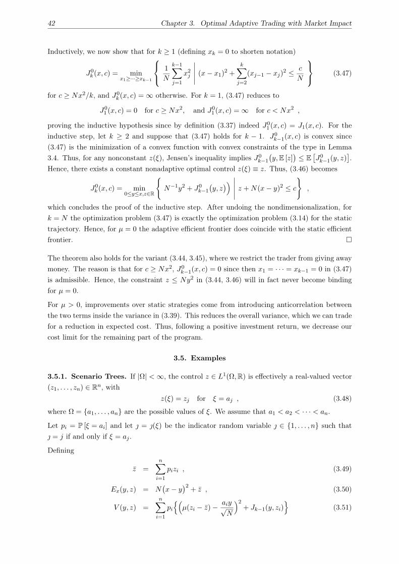
42 Chapter 3. Optimal Adaptive Trading with Market Impact
Inductively, we now show that for k ≥ 1 (defining xk = 0 to shorten notation)
J0k (x, c) = min
x1≥···≥xk−1
1
N
k−1∑
j=1
x2j
∣∣∣∣∣ (x− x1)2 +
k∑
j=2
(xj−1 − xj)2 ≤ c
N
(3.47)
for c ≥ Nx2/k, and J0k (x, c) =∞ otherwise. For k = 1, (3.47) reduces to
J01 (x, c) = 0 for c ≥ Nx2, and J0
1 (x, c) =∞ for c < Nx2 ,
proving the inductive hypothesis since by definition (3.37) indeed J01 (x, c) = J1(x, c). For the
inductive step, let k ≥ 2 and suppose that (3.47) holds for k − 1. J0k−1(x, c) is convex since
(3.47) is the minimization of a convex function with convex constraints of the type in Lemma
3.4. Thus, for any nonconstant z(ξ), Jensen’s inequality implies J0k−1
(y, E [z]
)≤ E
[J0
k−1(y, z)].
Hence, there exists a constant nonadaptive optimal control z(ξ) ≡ z. Thus, (3.46) becomes
J0k (x, c) = min
0≤y≤x,z∈R
N−1y2 + J0
k−1
(y, z))∣∣∣∣∣ z + N(x− y)2 ≤ c
,
which concludes the proof of the inductive step. After undoing the nondimensionalization, for
k = N the optimization problem (3.47) is exactly the optimization problem (3.14) for the static
trajectory. Hence, for µ = 0 the adaptive efficient frontier does coincide with the static efficient
frontier.
The theorem also holds for the variant (3.44, 3.45), where we restrict the trader from giving away
money. The reason is that for c ≥ Nx2, J0k−1(x, c) = 0 since then x1 = · · · = xk−1 = 0 in (3.47)
is admissible. Hence, the constraint z ≤ Ny2 in (3.44, 3.46) will in fact never become binding
for µ = 0.
For µ > 0, improvements over static strategies come from introducing anticorrelation between
the two terms inside the variance in (3.39). This reduces the overall variance, which we can trade
for a reduction in expected cost. Thus, following a positive investment return, we decrease our
cost limit for the remaining part of the program.
3.5. Examples
3.5.1. Scenario Trees. If |Ω| <∞, the control z ∈ L1(Ω, R) is effectively a real-valued vector
(z1, . . . , zn) ∈ Rn, with
z(ξ) = zj for ξ = aj , (3.48)
where Ω = a1, . . . , an are the possible values of ξ. We assume that a1 < a2 < · · · < an.
Let pi = P [ξ = ai] and let = (ξ) be the indicator random variable ∈ 1, . . . , n such that
= j if and only if ξ = aj .
Defining
z =n∑
i=1
pizi , (3.49)
Ex(y, z) = N(x− y
)2+ z , (3.50)
V (y, z) =n∑
i=1
pi
(µ(zi − z)− aiy√
N
)2+ Jk−1(y, zi)
(3.51)

3.5. Examples 43
Efficient frontierfor x shares and k periods
c z0 z+z-
x j < 0
x j > 0
......
E[C]
Efficient frontierfor x’ shares and k-1 periods
Var[C] Var[C]
E[C]
Figure 3.2. Illustration of the backwards optimization in the binomial model in
Section 3.5. If we already have the efficient frontiers to sell in (k− 1) periods and
want to compute the efficient frontier to sell in k periods, we need to determine
an optimal control (y, z+, z−): we sell x−y shares in the first period, and commit
ourselves to trading strategies for the remaining (k−1) periods – chosen from the
set of (k− 1)-period efficient strategies depending on whether the stock goes up or
down. If the stock goes up, we follow the efficient strategy with expected cost z+.
If it goes down, we follow the efficient strategy with expected cost z−. The coice
z+ = z− = z0 would lead to a path-independent strategy. By choosing z+ > z−
(and y) optimally, we can reduce the variance of the whole strategy – measured at
the beginning of the k-period trading time window. Instead of the square shaped
point on the static k-period frontier, we obtain a point on the improved k-period
frontier (blue dashed line).
the optimization problem (3.38,3.39) reads
Jk(x, c) = min(y,z1,...,zn)∈Rn+1
V (y, z)
∣∣∣∣∣∣∣∣∣∣
Ex(y, z) ≤ c (C1)
Ny2
k − 1≤ zi, i = 1 . . . n (C2)
0 ≤ y ≤ x (C3)
(3.52)
in dom Jk = (x, c) | x ≥ 0, c ≥ Nx2/k, with the terminal value function J1(x, c) in (3.37).
Thus, we have to solve an optimization problem with n + 1 variables in each step.
In the simplest example, we set Ω = ±1, i.e. n = 2. That is, we consider a binomial tree where
the stock price goes either up or down one tick during each of the N trading periods. Figure 3.2
illustrates the resulting binomial adaptivity model.
The corresponding dynamic program (3.44, 3.45) for J ′(x, c), defined in (3.43), is given by
J ′k(x, c) = min
(y,z1,...,zn)∈Rn+1
V (y, z)
∣∣∣∣∣∣∣∣∣∣∣∣∣
Ex(y, z) ≤ c (C1)
Ny2
k − 1≤ zi, i = 1 . . . n (C2)
0 ≤ y ≤ x (C3)
Ny2 ≥ zi, i = 1 . . . n (C4)
, (3.53)
where we now have the additional constraint (C4). The terminal value function J ′1(x, c) = J1(x, c)
remains unchanged. As (3.44,3.45), (3.53) does not consitute a convex problem due to the non-
convex constraint (C4).

44 Chapter 3. Optimal Adaptive Trading with Market Impact
3.5.2. Aggressiveness In-the-money (AIM) of Optimal Adaptive Policies. In this sec-
tion we shall prove that for an optimal adaptive policy the control z(ξ) is positively correlated
to the stock price return.
In terms of the controls z1, . . . , zn this means that z1 ≤ · · · ≤ zn since by definition (3.48) for
i < j, the control zi corresponds to a price change ξ that is smaller than for zj . The interpretation
is that if the stock price goes up, we sell faster (higher expected cost zi for the remainder). As in
Chapter 2, we obtain a AIM strategy (aggressive in the money), which burns part of the windfall
trading gains to sell faster and reduce the risk for the time left.
Theorem 3.8. Let µ > 0 and 3 ≤ k ≤ N . For Nx2/k < c < Nx2 the optimal control for
Jk(x, c) in (3.49,3.50,3.51,3.52) satisfies
y > 0 and z1 ≤ z2 ≤ · · · ≤ zk . (3.54)
For c ≥ Nx2, the optimal control is y = z1 = · · · = zk = 0 (immediate liquidation) and for
c = Nx2/k it is y = (k − 1)x/k and z1 = · · · = zk = x2(k − 1)N/k2 (linear profile).
Proof. It is easy to see that for c ≥ Einst = Nx2 we have Jk(x, c) = 0 with optimal control
y = z1 = · · · = zk = 0. For c = Nx2/k, the only point that satisfies (C1)–(C3) in (3.52) is
y = (k − 1)x/k and z1 = · · · = zk = x2(k − 1)N/k2, which indeed corresponds to the linear
strategy.
For c < Nx2, suppose y = 0. Then, by (3.50) we have Ex(y, z) ≥ Nx2, a contradiction.
We prove z1 ≤ z2 ≤ · · · ≤ zk by contradiction as well. Suppose zs > zr for r > s. Let
z =przr + pszs
pr + psand δ = zr − zs .
Then δ < 0, and
zr = z +ps
pr + psδ and zs = z − pr
pr + psδ . (3.55)
Let
A = µ
n∑
j=1
pjzj = (pr + ps)µz + µ∑
j 6=r,s
pjzj ,
and
∆ = V (y, z1, . . . , zn)− V (y, z1, . . . , zn) (3.56)
with zi = zi for i /∈ r, s and zr = zs = z. Since Ex(y, z1, . . . , zn) = Ex(y, z1, . . . , zn), the control
(y, z1, . . . , zn) satisfies (C1) in (3.52). Since z satisfies (C2) in (3.52), i.e. zr ≥ y2N/(k − 1), we
have z > zr ≥ y2N/(k − 1), and hence z also satisfies (C2).
We shall prove that ∆ < 0, contradicting the optimality of (y, z1, . . . , zn). To shorten notation,
let J(x, c) = Jk−1(x, c).
Since J(x, c) is convex,
prJ(y, zr) + psJ(y, zs) ≥ (pr + ps)J(y,
przr + pszs
pr + ps
)= (pr + ps)J(y, z) .
3.5. Examples 45
Hence,
∆ =∑
i=r,s
pi
[(µz − yai√
N−A
)2 −(µzi −
yai√N−A
)2+ J(y, z)− J(y, zi)
],
≤∑
i=r,s
pi
[(µz − yai√
N−A
)2 −(µzi −
yai√N−A
)2].
Because of (3.55),
(µz − yar√
N−A
)2 −(µzr −
yar√N−A
)2= −2
(µz − yar√
N−A
) µpsδ
pr + ps− p2
sδ2
(pr + ps)2
and
(µz − yas√
N−A
)2 −(µzs −
yas√N−A
)2= 2(µz − yas√
N−A
) µprδ
pr + ps− p2
rδ2
(pr + ps)2.
Thus,
∆ ≤ −(prp2s + psp
2r)δ
2µ2
(pr + ps)2− 2prpsδµ
pr + ps
y(as − ar)√N
≤ 2prpsµ
(pr + ps)√
Nδy(ar − as) .
Since ar > as, δ < 0 and y > 0 (as shown above), we conclude ∆ < 0, which completes the
proof.
In the Markowitz portfolio problem in a multiperiod setting that we shall consider in Chapter 5,
where a closed-form analytical solution for the dynamic program can be obtained, the optimal
control function z : Ω → R is perfectly anti-correlated to the portfolio return in the current
period. Unfortunately, this argument cannot be used for (3.37, 3.38, 3.39) because we effectively
have the constraint “z ≥ Elin(x, k)” (this is enforced by Jk(x, c) = ∞ for all z < Elin(x, k) by
the definition the the value function (3.19, 3.20), which is also easily verified inductively for the
dynamic program). Since in general the stock price change ξ may take arbitrarily large positive
and negative values, a lower bounded z can never be perfectly correlated to ξ.
3.5.3. Approximation of Optimal Control. If |Ω| is very large, or we even have |Ω| = ∞(for instance, if ξ ∼ N (0, 1)), approximate solutions can be obtained by restricting the space of
admissible controls instead of considering all measurable functions on Ω. In the following, we
assume Ω ⊆ R.
We partition the real line into n intervals I1, . . . , In with
I1 = (−∞, a1), I2 = [a1, a2), . . . , In−1 = [an−1, an), In = [an,∞)
for a1 < · · · < an. For given (z1, . . . , zn) ∈ Rn we define the step function z : R→ R by
z(ξ) = zj for ξ ∈ Ij .
We want to approximate the space of all measurable functions on Ω by considering only step
functions of this type. Not least due to the recursive structure of the dynamic program, formal
convergence is not obvious, and we leave this as an open question. In practice, this scheme will
certainly yield good results.

46 Chapter 3. Optimal Adaptive Trading with Market Impact
We let pi = P [ξ ∈ Ii], Ei = E [ξ | ξ ∈ Ii] and Vi = Var [ξ | ξ ∈ Ii], and now define the indicator
random variable = (ξ) such that = j if and only if ξ ∈ Ij .
By the law of total variance in Lemma 3.1, we obtain
Var
[µz −
ξy√N
]= Var
[E
[µz −
ξy√N
∣∣∣∣∣ ]]
+ E
[Var
[µz −
ξy√N
∣∣∣∣∣ ]]
= Var
[µz −
yE√N
]+ E
[y2V
N
]
=n∑
i=1
pi
(µzi −
Eiy√N− µ
n∑
j=1
pjzj
)2
+y2
N
n∑
i=1
piVi .
Similar to (3.49, 3.50, 3.51, 3.52), we define
z =n∑
i=1
pizi ,
Ex(y, z) = N(x− y
)2+ z ,
V (y, z) =n∑
i=1
pi
(µ(zi − z)− Eiy√
N
)2+
y2Vi
N+ Jk−1(y, zi)
and the optimization problem now reads
Jk(x, c) = min(y,z1,...,zn)∈Rn+1
V (y, z)
∣∣∣∣∣∣∣∣∣∣
Ex(y, z) ≤ c (C1)
Ny2
k − 1≤ zi, i = 1 . . . n (C2)
0 ≤ y ≤ x (C3)
.
An approximation of the variant J ′(x, c) is obtained analogously.
The simplest case of an approximation of this type is to consider a binomial framework: set
n = 2 with a1 = 0 (I1 = (−∞, 0) and I2 = [0,∞)), i.e. only respond to whether ξ ≥ 0 or ξ < 0.
3.5.4. Numerical Results. For numerical computations, we discretize the state space of the
value functions Jk(x, c). The figures presented in this section were generated for T = 1, N = 50
time steps (i.e. τ = 1/50) with Nx = 150 grid points for the relative portfolio size x ∈ [0, 1]
and Nc = 150 in the cost dimension (i.e. Nc points on the frontier for each value of x). We use
ξ ∼ N (0, 1) and the approximation of the optimal controls described in Section 3.5.3 with n = 2
and a1 = 0. Starting with J1(x, c), we successively determine J2(x, c), . . . , JN (x, c) by means
of (3.52), using interpolated values from the grid data of the previous value function. We use
standard direct search methods to find the optimal control (y, z+, z−). Since the optimization
problem is convex, local minima are global optimal solutions. For each level of x we have to trace
an efficient frontier. The function value (3.11) for the linear strategy at the upper-left end of the
frontier is readily available; from there, we work towards the right (increasing c) and compute
optimal controls for each c by taking the optimal controls for the point c − h (where h is the
discretization along the cost dimension) as the starting point for the iteration. Note that the
optimal control for c − h is indeed a feasible starting point for the optimization problem with
maximal cost c.
3.5. Examples 47
Figure 3.4 shows the set of efficient frontiers at the initial time t = 0 for the entire initial
portfolio (i.e. relative portfolio size x = 1) for different values of the market power 0 ≤ µ ≤ 0.15.
(Recall the discussion about the order of magnitude for µ in Section 3.4.2.) The x-axis is the
expectation of total cost, and the y-axis its variance. We scale both, expectation and variance,
by their values for the linear trajectories (see (3.11)). The two blue marks on the frontier for
µ = 0.15 correspond to optimal adaptive strategies with the same mean, but lower variance
(below the black mark) and same variance, but lower mean (to the left of the black mark) as
the static strategy corresponding to the black mark. The inset shows the cost distributions
associated with these three strategies (trading costs increase to the right of the x-axis). The
static cost distribution is readily available as a Gaussian with mean and variance according to its
location along the frontier. For the adaptive strategies, this is not the case. Since the solution of
the dynamic program is only the optimal strategy (given as a series of optimal one-step controls
as a function of the state variables), we determine the associated cost distributions by Monte
Carlo simulation. Suppose we want to simulate the strategy that has expected cost at most E
(measured at time t = 0). Then, using (3.27, 3.28, 3.22), for each of m = 105 randomly sampled
paths of the stock price (ξ1, . . . , ξN ) the final cost CN is obtained by sequentially applying
the optimal one-step controls (y∗k(x, c), z∗k±(x, c)) associated with Jk(xk, c) (respectively, their
interpolated values over the discretized state space),
xi+1 = y∗i (xi, ci)
ci+1 =
z∗i+(xi, ci) ξi+1 ≥ 0
z∗i−(xi, ci) ξi+1 < 0
Ci+1 = Ci + µN(xi − xi+1)2 − xi+1ξi+1/
√N
with x0 = 1, C0 = 0 and the initial limit c0 = E for the expected cost. Ci is measured in units
of σ√
TX, the standard deviation of the initial portfolio value due to the stock price volatility
across the trading horizon.
The adaptive cost distributions are slightly skewed, suggesting that mean-variance optimization
may not give the best possible solutions. Figure 3.5 shows four static and adaptive cost distri-
butions along the frontier. In the upper left corner (near the linear strategy), the adaptive cost
distributions are almost Gaussian (Point #1); indeed, for high values of V adaptive and static
strategies coincide. As we move down the frontiers (towards less risk-averse strategies), the skew-
ness first increases (Point #2). Interestingly, as we move further down – where the improvement
of the adaptive strategy becomes larger – the adaptive distributions look more and more like
Gaussian again (Point #3 and #4). All adaptive distributions are strictly preferable to their
reference static strategy, since they have lower probability of high costs and higher probability of
low costs. Table 1 compares the semi-variance, value-at-risk (VaR) and conditional value-at-risk
(CVaR) (see Artzner, Delbaen, Eber, and Heath, 1999, for instance) for the four distribution
pairs shown in Figure 3.5. For Gaussian random variables, mean-variance is consistent with
expected utility maximization as well as stochastic dominance (see for instance Levy (1992);
Bertsimas et al. (2004)). As the adaptive distributions are indeed not too far from Gaussian, we
can expect mean-variance to give reasonable results.
48 Chapter 3. Optimal Adaptive Trading with Market Impact
One way to improve on this further would be to add constraints on the skewness to the op-
timization problem (3.9); for instance, we could require Skew [C(X, N, π)] ≥ 0. In fact, using
a generalization of Lemma 3.1 for higher central moments (“law of total cumulance”), such an
extension of the dynamic programming principle in Section 3.4 is indeed possible.
To illustrate the behavior of adaptive policies in the binomial framework, Figure 3.3 shows
trajectories for two sample paths of the stock price in a small instance with N = 4. The inset
shows the underlying binomial decision tree. As can be seen, the optimal adaptive policies are
indeed “aggressive in the money”. If the stock price goes up, we incur unexpectedly smaller total
trading cost and react with selling faster (burning some of the gains), whereas for falling stock
price, we slow down trading. Figure 3.6 shows optimal adaptive and static trading for N = 50.
The static strategy is chosen such that it has the same expected cost (yet higher variance) as
the adaptive policy.
The numerical results presented so far were obtained using the value function JN . Let us briefly
discuss the results for the value function definition J ′N . As mentioned there, J ′
N (x, c) ≥ JN (x, c).
In the specification of JN (respectively, E ) the trader can reduce his variance by destroying money
in order to make a positive outcome less so (see discussion in Section 3.4.3). In the specification
of J ′N (respectively, E ′) this is not possible. The numerical results show that while this effect is
important for small values of N and large values of µ (see Figure 3.8), it diminishes very rapidly
as N increases (see Figure 3.7). In fact, the value of µ = 2 in Figure 3.7 is very large (recall
our discussion for the order of µ in Section 3.4.2), and for realistic values of µ the difference
is even smaller. That is, while the specification of JN and E (X, N) allow for the undesirable
peculiarity that the trader gives away money in positive outcomes, our numerical results show
that this effect does not play a big role in practice. Compared to J ′N , the specification of JN has
the big advantage that the associated dynamic program is convex, which makes the numerical
optimization significantly easier.
3.5.5. Comparison with Results of Single-update Strategies. It is interesting to compare
the improvement of the optimal adaptive strategy with the improvement obtained by the single
update strategies from Chapter 2. Before doing so, let us first stress that the single update
framework presented in the previous chapter is formulated in the continuous-time version of the
Almgren/Chriss model, whereas the solution obtained with the dynamic programming technique
in this chapter works in the discrete-time version. As mentioned in Section 3.2, for τ → 0 the
discrete time model converges to a continuous-time model, but for τ ≫ 0 the two models differ.
In the following let us refer to the optimal adaptive strategy from this chapter (in the binomial
framework) with N = 50 time steps as strategy M (“Multi-Update”), and to the single update
strategy (with n = 2 there) from the previous chapter as strategy S (“Single-Update”).
Figures 2.2 and 3.4 show the improved efficient frontiers for the same values of µ for both
strategies. Expectation and variance are measured relative to the cost of the respective linear
strategy, i.e. the linear strategy in continuous-time for strategy S (Figure 2.2) and the linear
strategy in discrete-time strategy M (Figure 3.4). The sample distributions shown in the insets
in both figures use a static strategy with mean E = 7.00 ·Elin, and variance V = 0.107 · Vlin (in
case of strategy S, Figure 2.2) and V = 0.0884 · Vlin (in case of strategy M, Figure 3.4); note

3.5. Examples 49
0 1 2 3 40
0.1
0.2
0.3
0.4
0.5
0.6
0.7
0.8
0.9
1
t
Sha
res
rem
aini
ng x
(t)
0 1 2 3 4
S(t)−S0
t
Figure 3.3. Optimal adaptive trading for N = 4 time steps, illustrating the
binomial adaptivity model. The blue trajectory corresponds to the rising stock
price path, and sells faster than red trajectory (falling stock price path). The
inset shows the schematics of the stock price on the binomial tree. x1 at t = 1 is
the same for all adaptive trajectories because x1 is determined at t = 0 with no
information available. Only from t = 1 onwards the adaptive trajectories split.
that the difference in variance (for the same level of expected cost) is due to the slightly different
models (discrete-time vs. continuous-time). For strategy M (Figure 3.4), the two improved
adaptive distributions have mean and variance of (E = 4.00 · Elin, V = 0.0884 · Vlin) and (E =
7.00 · Elin, V = 0.0334 · Vlin). For strategy S (Figure 3.4), the improved adaptive distributions
have mean and variance of (E = 4.47·Elin, V = 0.107·Vlin) and (E = 7.00·Elin, V = 0.0612·Vlin).
Figure 3.9 shows the entire efficient frontiers (with µ = 0.15) for the two models, single-update
in continuous-time (Chapter 2) and multi-update discrete-time (Chapter 3) compared to their
corresponding static frontiers.
Due to the difference between the continuous-time and the discrete-time model those values have
to be approached with caution. However, it is evident that single update strategies achieve a
relative improvement that is already comparable to the improvement of the adaptive strategies
developed in this chapter. Thus, from a practical point of view the single-update framework is
indeed attractive, as the computational cost for solving the single-step optimization problem is
naturally much less than for solving the dynamic program.
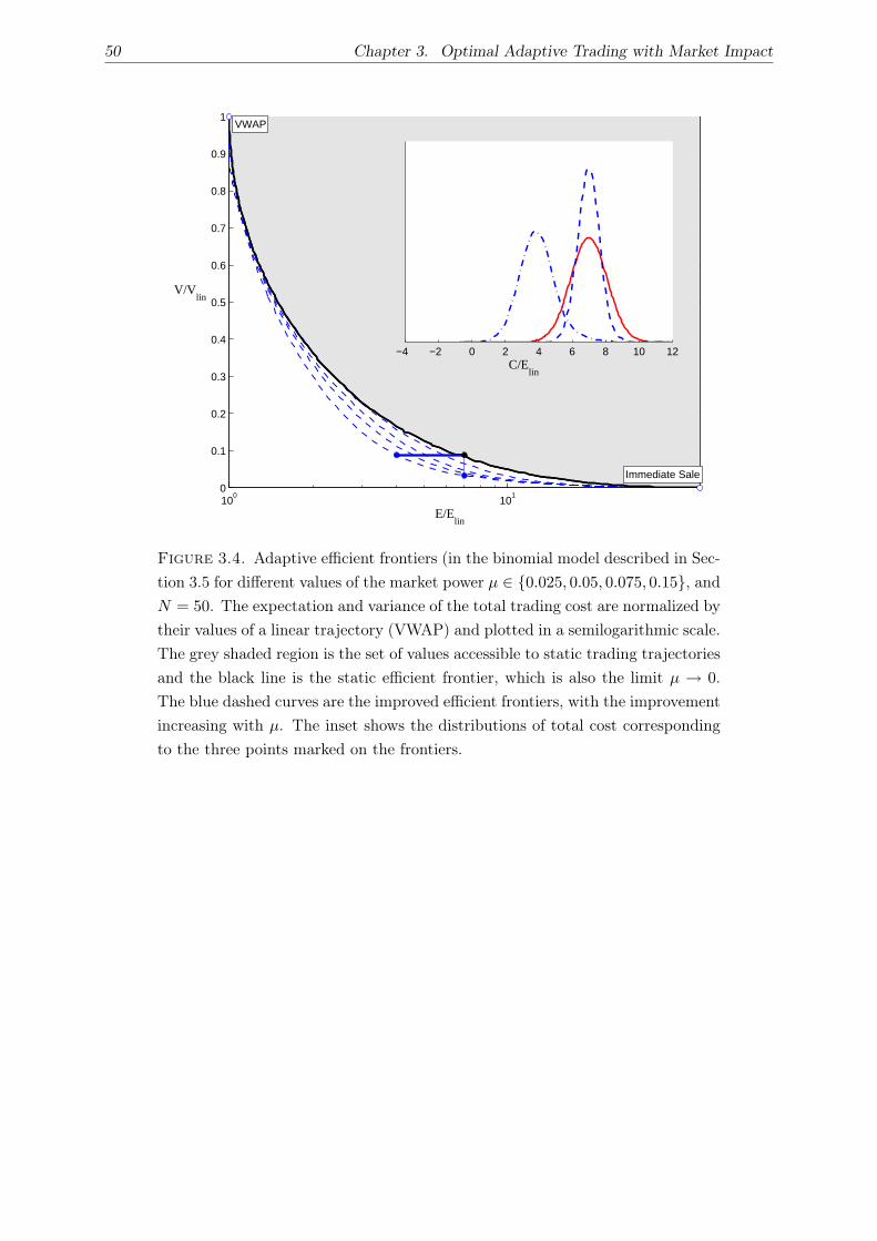
50 Chapter 3. Optimal Adaptive Trading with Market Impact
100
101
0
0.1
0.2
0.3
0.4
0.5
0.6
0.7
0.8
0.9
1
E/Elin
V/Vlin
VWAP
Immediate Sale
−4 −2 0 2 4 6 8 10 12C/E
lin
Figure 3.4. Adaptive efficient frontiers (in the binomial model described in Sec-
tion 3.5 for different values of the market power µ ∈ 0.025, 0.05, 0.075, 0.15, and
N = 50. The expectation and variance of the total trading cost are normalized by
their values of a linear trajectory (VWAP) and plotted in a semilogarithmic scale.
The grey shaded region is the set of values accessible to static trading trajectories
and the black line is the static efficient frontier, which is also the limit µ → 0.
The blue dashed curves are the improved efficient frontiers, with the improvement
increasing with µ. The inset shows the distributions of total cost corresponding
to the three points marked on the frontiers.

3.5. Examples 51
100
101
0
0.1
0.2
0.3
0.4
0.5
0.6
0.7
0.8
0.9
1
E/Elin
V/Vlin
VWAP
Immediate Sale
1
2
3
4
−5 0 5 10C/E
lin
Point #1 on frontier
0 5 10C/E
lin
Point #2 on frontier
2 4 6 8 10C/E
lin
Point #3 on frontier
6 8 10 12 14C/E
lin
Point #4 on frontier
Figure 3.5. Distributions of total cost corresponding to four points on the fron-
tier, µ = 0.15 and N = 50. The adaptive distributions are reasonably close to
Gaussian; recall that the static distribution functions are always exactly Gaussian
by construction.

52 Chapter 3. Optimal Adaptive Trading with Market Impact
#1 #2 #3 #4
static adapt static adapt static adapt static adapt
E [·] 1.68 1.52 2.96 2.27 7.00 3.92 13.00 7.09
Var [·] 5.98 5.98 3.19 3.19 1.20 1.20 0.44 0.44
SVar[·] 3.01 3.35 1.61 1.89 0.60 0.68 0.22 0.22
VaR5.0% 5.70 5.85 5.90 5.58 8.80 5.83 14.09 8.17
VaR2.5% 6.47 6.77 6.46 6.38 9.14 6.34 14.29 8.41
VaR1.0% 7.37 7.91 7.12 7.35 9.54 7.02 14.54 8.73
VaR0.5% 7.98 8.62 7.56 8.00 9.82 7.56 14.70 8.97
VaR0.1% 9.23 10.18 8.48 9.45 10.38 8.57 15.04 9.43
CVaR5.0% 6.72 7.09 6.65 6.67 9.25 6.56 14.36 8.51
CVaR2.5% 7.43 7.91 7.15 7.39 9.57 7.06 14.54 8.75
CVaR1.0% 8.23 8.87 7.71 8.26 9.93 7.71 14.77 9.06
CVaR0.5% 8.76 9.52 8.14 8.87 10.20 8.19 14.91 9.28
CVaR0.1% 9.94 10.96 8.97 10.16 10.69 9.19 15.20 9.80
Table 1. Statistics for the adaptive and static cost distribution functions shown
in Figure 3.5, obtained by Monte Carlo simulation (105 sample paths). For the
random variable C, the total cost in units of Elin, the value-at-risk VaRβ is
defined by P [C ≥ VaRβ(C)] = β, and the conditional-value-at-risk CVaRβ(C) =
E [C |C ≥ VaRβ(C)]. Thus, low values for VaR and CVaR are desirable.
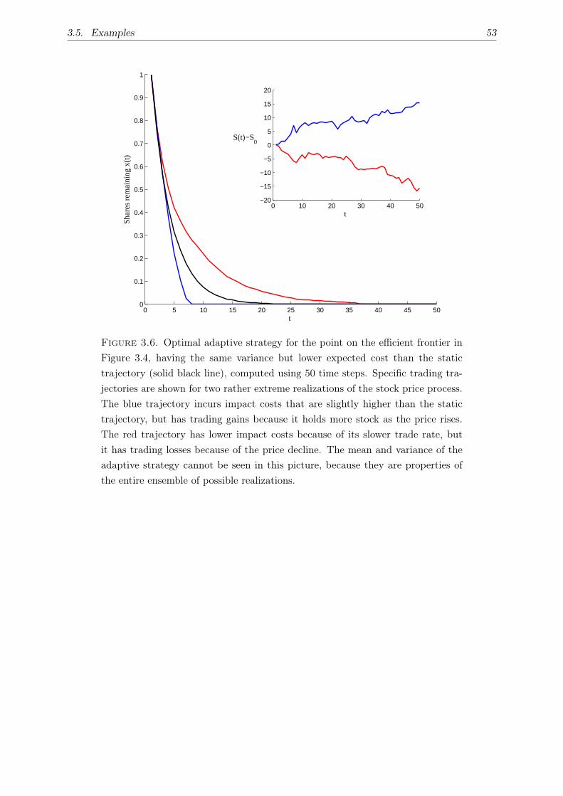
3.5. Examples 53
0 5 10 15 20 25 30 35 40 45 500
0.1
0.2
0.3
0.4
0.5
0.6
0.7
0.8
0.9
1
t
Sha
res
rem
aini
ng x
(t)
0 10 20 30 40 50−20
−15
−10
−5
0
5
10
15
20
t
S(t)−S0
Figure 3.6. Optimal adaptive strategy for the point on the efficient frontier in
Figure 3.4, having the same variance but lower expected cost than the static
trajectory (solid black line), computed using 50 time steps. Specific trading tra-
jectories are shown for two rather extreme realizations of the stock price process.
The blue trajectory incurs impact costs that are slightly higher than the static
trajectory, but has trading gains because it holds more stock as the price rises.
The red trajectory has lower impact costs because of its slower trade rate, but
it has trading losses because of the price decline. The mean and variance of the
adaptive strategy cannot be seen in this picture, because they are properties of
the entire ensemble of possible realizations.

54 Chapter 3. Optimal Adaptive Trading with Market Impact
1 1.2 1.4 1.6 1.8 20
0.1
0.2
0.3
0.4
0.5
0.6
0.7
0.8
0.9
1N=2
c / Elin
J N(1
,c)
/ Elin
1 1.5 2 2.5 30
0.2
0.4
0.6
0.8
1
1.2
1.4N=3
c / Elin
J N(1
,c)
/ Elin
1 1.5 2 2.5 3 3.5 40
0.2
0.4
0.6
0.8
1
1.2
1.4N=4
c / Elin
J N(1
,c)
/ Elin
2 3 4 5 6 7 8 910
−4
10−3
10−2
10−1
N
|JN
−J´
|
Figure 3.7. The first three plots show JN (x, c) (blue solid line) vs. J ′N (x, c)
(black solid line) for N = 2, 3, 4 and µ = 2. For N = 2, the two curves are clearly
separated. For N = 3 there is only a very small visible difference for larger values
of c (around c/Elin ≈ 2), and for N = 4 the two curves are practically identical.
The dashed line is the static frontier (µ = 0), which coincides for N = 2 with J ′2.
The last plot shows ‖JN − J ′N‖1 as function of N in semilogarithmic scale.
1 1.2 1.4 1.6 1.8 20
0.1
0.2
0.3
0.4
0.5
0.6
0.7
0.8
0.9
1
c / Elin
J 2´(1,
c) /
Elin
0 1 2 3 4 50
0.01
0.02
0.03
0.04
0.05
0.06
0.07
0.08
0.09
mu
|J2−
J´|
Figure 3.8. Left plot shows J2(x, c) for different values of µ ∈0.25, 0.5, 0.75, 1.0 as a function of c (and x = 1). The black line is J ′
2(x, c).
The right plot shows ‖J2 − J ′2‖1 as a function of µ.

3.5. Examples 55
100
101
0
0.1
0.2
0.3
0.4
0.5
0.6
0.7
0.8
0.9
1 VWAP
E/Elin
V/V
lin
SS
SA
MS
MA
Single−Update Strategy (Chapter 2)Dynamic Program Strategy (Chapter 3)
Figure 3.9. The blue solid line (labeled SS) is the static frontier (i.e. µ = 0) in
the continuous-time model of Chapter 2, and the red solid line (MS) is the static
frontier in the discrete-time setting of Chapter 3 (with N = 50 time steps). Due
to the discretization effect, the two frontiers are not exactly the same. The dashed
red curve (SA) and blue curve (MA) are the adaptive frontiers in the two models,
both for µ = 0.15. All values are scaled by their values of the corresponding linear
strategies (in the continuous-time and discrete-time model, respectively).


CHAPTER 4
Bayesian Adaptive Trading with Price Appreciation
In this chapter, we discuss a model that incorporates another major source of slippage besides
market impact, namely price appreciation. As proposed in Section 1.3, we consider a model in
which the trader uses information from observations of the price evolution during the day to
continuously update his estimate of the price momentum resulting from other traders’ target
sizes and directions. The motivation for this model is the daily trading cycle: large institutional
traders make investment decisions in the morning and implement them through the trading day.
Using this information we determine optimal trade schedules to minimize total expected cost of
trading.
4.1. Introduction
Most current models of optimal trading strategies view time as an undifferentiated continuum,
and other traders as a collection of random noise sources. Trade decisions are made at random
times and trade programs have random durations. Thus, if one observes buy pressure from the
market as a whole, one has no reason to believe that this pressure will last more than a short
time. From the point of view of optimal trading, price motions are purely random.
Here we present a model for price dynamics and optimal trading that explicitly includes the
daily trading cycle: large institutional participants make investment decisions overnight and
implement them through the following trading day. Within each day, the morning is different
from the afternoon, since an intelligent trader will spend the early trading hours collecting
information about the targets of other traders, and will use this information to trade in the rest
of the day. His main source of information is the observation of the price dynamics.
As in Chapters 2 and 3, this will result in an adaptive execution algorithm. However, in the
previous chapter we assumed a pure random walk model with no price momentum or serial
correlation, using pure classic mean variance. The adaptive behavior discovered there stems from
the trader’s risk-aversion. In this chapter we consider a risk-neutral trader, whose motivation for
accelerating or slowing down trading is the momentum of the asset price.
The following model may be interpreted as one plausible way to model such price momentum
that the trader observes during the course of the day. There is an underlying drift factor, caused
by the net positions being executed by other institutional investors. This factor is approximately
constant throughout the day because other traders execute across the entire day. Thus price
increases in the early part of the day suggest that this factor is positive, which suggests that
prices will continue to increase throughout the day. This is different from a short-term momentum
model in which the price change across one short period of time is correlated with the price change
across a preceding period; most empirical evidence shows that such correlation is weak if it exists
57
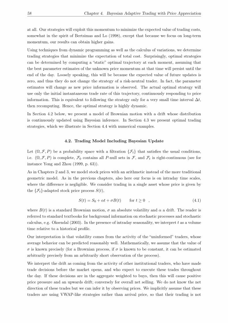
58 Chapter 4. Bayesian Adaptive Trading with Price Appreciation
at all. Our strategies will exploit this momentum to minimize the expected value of trading costs,
somewhat in the spirit of Bertsimas and Lo (1998), except that because we focus on long-term
momentum, our results can obtain higher gains.
Using techniques from dynamic programming as well as the calculus of variations, we determine
trading strategies that minimize the expectation of total cost. Surprisingly, optimal strategies
can be determined by computing a “static” optimal trajectory at each moment, assuming that
the best parameter estimates of the unknown price momentum at that time will persist until the
end of the day. Loosely speaking, this will be because the expected value of future updates is
zero, and thus they do not change the strategy of a risk-neutral trader. In fact, the parameter
estimates will change as new price information is observed. The actual optimal strategy will
use only the initial instantaneous trade rate of this trajectory, continuously responding to price
information. This is equivalent to following the strategy only for a very small time interval ∆t,
then recomputing. Hence, the optimal strategy is highly dynamic.
In Section 4.2 below, we present a model of Brownian motion with a drift whose distribution
is continuously updated using Bayesian inference. In Section 4.3 we present optimal trading
strategies, which we illustrate in Section 4.4 with numerical examples.
4.2. Trading Model Including Bayesian Update
Let (Ω,F , P ) be a probability space with a filtration Ft that satisfies the usual conditions,
i.e. (Ω,F , P ) is complete, F0 contains all P -null sets in F , and Ft is right-continuous (see for
instance Yong and Zhou (1999, p. 63)).
As in Chapters 2 and 3, we model stock prices with an arithmetic instead of the more traditional
geometric model. As in the previous chapters, also here our focus is on intraday time scales,
where the difference is negligible. We consider trading in a single asset whose price is given by
the Ft-adapted stock price process S(t),
S(t) = S0 + αt + σB(t) for t ≥ 0 , (4.1)
where B(t) is a standard Brownian motion, σ an absolute volatility and α a drift. The reader is
referred to standard textbooks for background information on stochastic processes and stochastic
calculus, e.g. Oksendal (2003). In the presence of intraday seasonality, we interpret t as a volume
time relative to a historical profile.
Our interpretation is that volatility comes from the activity of the “uninformed” traders, whose
average behavior can be predicted reasonably well. Mathematically, we assume that the value of
σ is known precisely (for a Brownian process, if σ is known to be constant, it can be estimated
arbitrarily precisely from an arbitrarily short observation of the process).
We interpret the drift as coming from the activity of other institutional traders, who have made
trade decisions before the market opens, and who expect to execute these trades throughout
the day. If these decisions are in the aggregate weighted to buys, then this will cause positive
price pressure and an upwards drift; conversely for overall net selling. We do not know the net
direction of these trades but we can infer it by observing prices. We implicitly assume that these
traders are using VWAP-like strategies rather than arrival price, so that their trading is not

4.2. Trading Model Including Bayesian Update 59
“front-loaded”. This assumption is questionable; if the strategies are front-loaded then the drift
coefficient would vary through the day.
Thus we assume that the drift α is constant throughout the day, but we do not know its value.
At the beginning of the day, we have a prior belief
α ∼ N(α, ν2
), (4.2)
which will be updated using price observations during the day. There are thus two sources
of randomness in the problem: the continuous Brownian motion representing the uninformed
traders, and the single drift coefficient representing the constant trading of the large traders.
4.2.1. Bayesian Inference. Intuitively, as the trader observes prices from the beginning of the
day onwards, he starts to get a feeling for the day’s price momentum.
More precisely, at time t we know the stock price trajectory S(τ) for 0 ≤ τ ≤ t. We have the
following result to update our estimate of the drift, given the observation S(τ) | 0 ≤ τ ≤ t.
Lemma 4.1. Given the observation S(τ) |0 ≤ τ ≤ t up to time t ≥ 0, we have the posterior
distribution for α,
α ∼ N(α, ν2
)(4.3)
with
α =ασ2 + ν2
(S(t)− S0
)
σ2 + ν2tand ν2 =
σ2
σ2 + ν2tν2 . (4.4)
Proof. In differential form, (4.1) reads
dS = αdt + σdB, S(0) = S0 . (4.5)
It follows from the work of Liptser and Shiryaev (2001, chap. 17.7) that for this diffusion process
the changes in the conditional expectation α(τ) = Eτ [α] and conditional variance v(τ) = ν(τ)2 =
Varτ [α] are given by the dynamics
dα =v(τ)
σ2
(dS − α(τ) dτ
), α(0) = α (4.6)
dv = −v(τ)2
σ2dτ, v(0) = ν2 . (4.7)
From (4.7) we immediately obtain
v(τ) =ν2σ2
σ2 + ν2τ,
and since ν2 = v(t), we have shown the second part of (4.4).
The solution to the SDE (4.6) for α is given by
α =ασ2 + ν2
(S(τ)− S0
)
σ2 + ν2τ, (4.8)
which is easily verified by Ito’s Lemma: For α = f(τ, S) =ασ2+ν2
(S−S0
)
σ2+ν2τ, Ito’s Lemma yields
dα =
(∂f
∂τ+ α
∂f
∂S+
1
2σ2 ∂2f
∂S2
)dτ + σ
∂f
∂SdB
(4.5)=
(∂f
∂τ+
1
2σ2 ∂2f
∂S2
)dτ +
∂f
∂SdS =
∂f
∂τdτ +
∂f
∂SdS . (4.9)
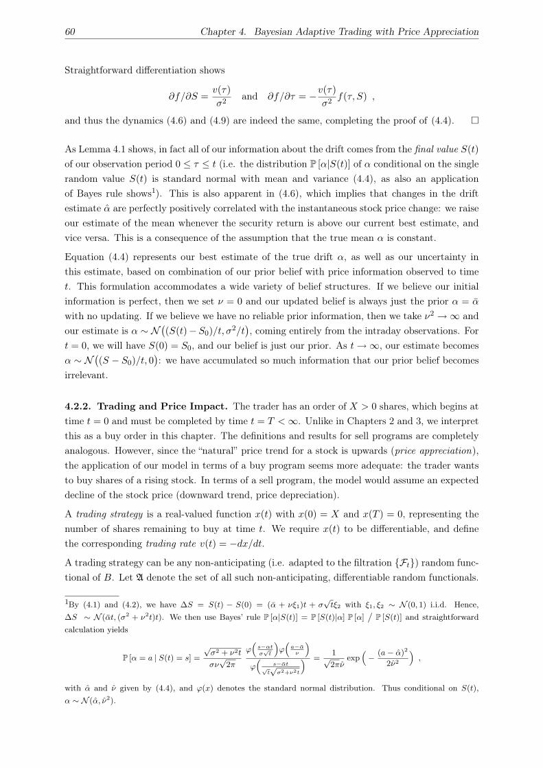
60 Chapter 4. Bayesian Adaptive Trading with Price Appreciation
Straightforward differentiation shows
∂f/∂S =v(τ)
σ2and ∂f/∂τ = −v(τ)
σ2f(τ, S) ,
and thus the dynamics (4.6) and (4.9) are indeed the same, completing the proof of (4.4).
As Lemma 4.1 shows, in fact all of our information about the drift comes from the final value S(t)
of our observation period 0 ≤ τ ≤ t (i.e. the distribution P [α|S(t)] of α conditional on the single
random value S(t) is standard normal with mean and variance (4.4), as also an application
of Bayes rule shows1). This is also apparent in (4.6), which implies that changes in the drift
estimate α are perfectly positively correlated with the instantaneous stock price change: we raise
our estimate of the mean whenever the security return is above our current best estimate, and
vice versa. This is a consequence of the assumption that the true mean α is constant.
Equation (4.4) represents our best estimate of the true drift α, as well as our uncertainty in
this estimate, based on combination of our prior belief with price information observed to time
t. This formulation accommodates a wide variety of belief structures. If we believe our initial
information is perfect, then we set ν = 0 and our updated belief is always just the prior α = α
with no updating. If we believe we have no reliable prior information, then we take ν2 →∞ and
our estimate is α ∼ N((S(t)− S0)/t, σ2/t
), coming entirely from the intraday observations. For
t = 0, we will have S(0) = S0, and our belief is just our prior. As t→∞, our estimate becomes
α ∼ N((S − S0)/t, 0
): we have accumulated so much information that our prior belief becomes
irrelevant.
4.2.2. Trading and Price Impact. The trader has an order of X > 0 shares, which begins at
time t = 0 and must be completed by time t = T <∞. Unlike in Chapters 2 and 3, we interpret
this as a buy order in this chapter. The definitions and results for sell programs are completely
analogous. However, since the “natural” price trend for a stock is upwards (price appreciation),
the application of our model in terms of a buy program seems more adequate: the trader wants
to buy shares of a rising stock. In terms of a sell program, the model would assume an expected
decline of the stock price (downward trend, price depreciation).
A trading strategy is a real-valued function x(t) with x(0) = X and x(T ) = 0, representing the
number of shares remaining to buy at time t. We require x(t) to be differentiable, and define
the corresponding trading rate v(t) = −dx/dt.
A trading strategy can be any non-anticipating (i.e. adapted to the filtration Ft) random func-
tional of B. Let A denote the set of all such non-anticipating, differentiable random functionals.
1By (4.1) and (4.2), we have ∆S = S(t) − S(0) = (α + νξ1)t + σ√
tξ2 with ξ1, ξ2 ∼ N (0, 1) i.i.d. Hence,
∆S ∼ N (αt, (σ2 + ν2t)t). We then use Bayes’ rule P [α|S(t)] = P [S(t)|α] P [α]‹
P [S(t)] and straightforward
calculation yields
P [α = a | S(t) = s] =
√σ2 + ν2t
σν√
2π
ϕ“
s−αt
σ√
t
”
ϕ“
a−αν
”
ϕ“
s−αt√t√
σ2+ν2t
” =1√2πν
exp“
− (a − α)2
2ν2
”
,
with α and ν given by (4.4), and ϕ(x) denotes the standard normal distribution. Thus conditional on S(t),
α ∼ N (α, ν2).
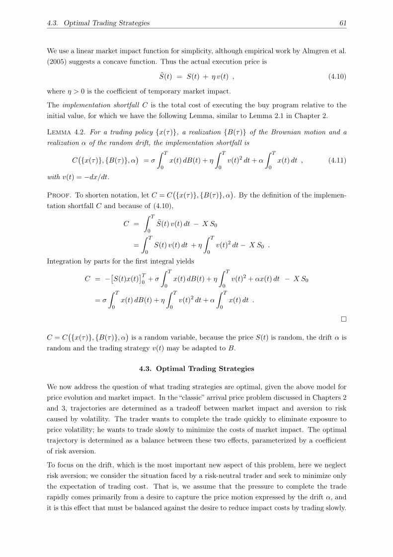
4.3. Optimal Trading Strategies 61
We use a linear market impact function for simplicity, although empirical work by Almgren et al.
(2005) suggests a concave function. Thus the actual execution price is
S(t) = S(t) + η v(t) , (4.10)
where η > 0 is the coefficient of temporary market impact.
The implementation shortfall C is the total cost of executing the buy program relative to the
initial value, for which we have the following Lemma, similar to Lemma 2.1 in Chapter 2.
Lemma 4.2. For a trading policy x(τ), a realization B(τ) of the Brownian motion and a
realization α of the random drift, the implementation shortfall is
C(x(τ), B(τ), α
)= σ
∫ T
0x(t) dB(t) + η
∫ T
0v(t)2 dt + α
∫ T
0x(t) dt , (4.11)
with v(t) = −dx/dt.
Proof. To shorten notation, let C = C(x(τ), B(τ), α
). By the definition of the implemen-
tation shortfall C and because of (4.10),
C =
∫ T
0S(t) v(t) dt − X S0
=
∫ T
0S(t) v(t) dt + η
∫ T
0v(t)2 dt− X S0 .
Integration by parts for the first integral yields
C = −[S(t)x(t)
]T0
+ σ
∫ T
0x(t) dB(t) + η
∫ T
0v(t)2 + αx(t) dt − X S0
= σ
∫ T
0x(t) dB(t) + η
∫ T
0v(t)2 dt + α
∫ T
0x(t) dt .
C = C(x(τ), B(τ), α
)is a random variable, because the price S(t) is random, the drift α is
random and the trading strategy v(t) may be adapted to B.
4.3. Optimal Trading Strategies
We now address the question of what trading strategies are optimal, given the above model for
price evolution and market impact. In the “classic” arrival price problem discussed in Chapters 2
and 3, trajectories are determined as a tradeoff between market impact and aversion to risk
caused by volatility. The trader wants to complete the trade quickly to eliminate exposure to
price volatility; he wants to trade slowly to minimize the costs of market impact. The optimal
trajectory is determined as a balance between these two effects, parameterized by a coefficient
of risk aversion.
To focus on the drift, which is the most important new aspect of this problem, here we neglect
risk aversion; we consider the situation faced by a risk-neutral trader and seek to minimize only
the expectation of trading cost. That is, we assume that the pressure to complete the trade
rapidly comes primarily from a desire to capture the price motion expressed by the drift α, and
it is this effect that must be balanced against the desire to reduce impact costs by trading slowly.

62 Chapter 4. Bayesian Adaptive Trading with Price Appreciation
To support this description, we shall generally suppose that the original buy decision was made
because the trader’s belief has α > 0. We then expect α > 0 in (4.11), and the term∫
α x(t) dt
is a positive cost. It may be that the true value has α < 0, or that intermediate price movements
cause us to form a negative estimate. Because our point of view is that of a broker/dealer
executing an agency trade, we shall always require that the trade be completed by t = T , unless
the instructions are modified.
Our trading goal is to determine a strategy that minimizes the expectation of the implementation
shortfall (4.11): determine x(τ) for 0 ≤ τ ≤ T so that
minx∈A
E[C(x(τ), B(τ), α
)]. (4.12)
This corresponds to determining optimal strategies for a risk-neutral trader.
4.3.1. Static Trajectories. Suppose at some intermediate time 0 ≤ t∗ < T we have x(t∗)
shares left to buy, and we decide to fix the trading strategy for the remaining time t∗ ≤ τ ≤ T
independently of B(τ) | t∗ ≤ τ ≤ T; regardless of the stock price process, we follow the same
trading trajectory. We will refer to such trading policies as static.
Lemma 4.3 gives optimal static trading strategies for a risk-neutral trader, i.e who optimizes
(4.12). The proof uses standard methods of the calculus of variations.
Lemma 4.3. Let 0 ≤ t∗ < T . Let α = α(t∗, S(t∗)) be our best estimate (4.4) of α at time t∗,
and let x(t∗) be the shares remaining to buy. Then for a risk-neutral trader the optimal static
strategy x(τ) | t∗ ≤ τ ≤ T specified at t = t∗ is given by
x(τ) =T − τ
T − t∗x(t∗) −
α
4η
(τ − t∗
)(T − τ
), t∗ ≤ τ ≤ T, (4.13)
and the instantaneous trade rate at time t∗ is
v(t∗) = −x′(τ)∣∣τ=t∗
=x(t∗)
T − t∗+
α
4η
(T − t∗
). (4.14)
The expectation of the remaining cost E[C(x(τ), B(τ), α
)]of the optimal static strategy
x(τ) | t∗ ≤ τ ≤ T is
E[C(x(τ), B(τ), α
)]=
x(t∗)2η
T − t∗+
x(t∗)α(T − t∗)
2− (T − t∗)
3α2
48η. (4.15)
Proof. Let x∗ = x(t∗) and let α = α(t∗, S(t∗)) be given by (4.4). For a static strategy
x(τ) | t∗ ≤ τ ≤ T specified at t∗, the final total cost C = C(x(τ), B(τ), α
)is a Gauss-
ian variable by Lemma 4.2. We want to determine a trajectory function x : [t∗, T ] → R with
endpoint conditions x(t∗) = x∗ and x(T ) = 0 to optimize
J [x] = E
[σ
∫ T
t∗x(t) dB(t) +
∫ T
t∗ηv(t)2 + αx(t) dt
∣∣∣∣∣ t∗
]
=
∫ T
t∗ηx′(t)2 + αx(t) dt , (4.16)
since E [α | t∗] = α. The Euler-Lagrange equation (see for instance Wan (1995)) for the variational
problem minJ [x] | x(t∗) = x∗, x(T ) = 0
is the ordinary differential equation
x′′(τ) =α
2η, t∗ ≤ τ ≤ T . (4.17)
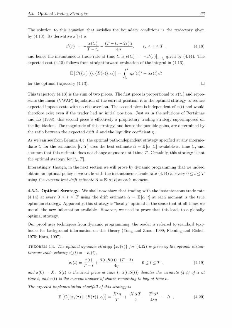
4.3. Optimal Trading Strategies 63
The solution to this equation that satisfies the boundary conditions is the trajectory given
by (4.13). Its derivative x′(τ) is
x′(τ) = − x(t∗)
T − t∗− (T + t∗ − 2τ)α
4η, t∗ ≤ τ ≤ T , (4.18)
and hence the instantaneous trade rate at time t∗ is v(t∗) = −x′(τ)∣∣τ=t∗
given by (4.14). The
expected cost (4.15) follows from straightforward evaluation of the integral in (4.16),
E[C(x(τ), B(τ), α
)]=
∫ T
t∗ηx′(t)2 + αx(t) dt
for the optimal trajectory (4.13).
This trajectory (4.13) is the sum of two pieces. The first piece is proportional to x(t∗) and repre-
sents the linear (VWAP) liquidation of the current position; it is the optimal strategy to reduce
expected impact costs with no risk aversion. The second piece is independent of x(t) and would
therefore exist even if the trader had no initial position. Just as in the solutions of Bertsimas
and Lo (1998), this second piece is effectively a proprietary trading strategy superimposed on
the liquidation. The magnitude of this strategy, and hence the possible gains, are determined by
the ratio between the expected drift α and the liquidity coefficient η.
As we can see from Lemma 4.3, the optimal path-independent strategy specified at any interme-
diate t∗ for the remainder [t∗, T ] uses the best estimate α = E [α | t∗] available at time t∗, and
assumes that this estimate does not change anymore until time T . Certainly, this strategy is not
the optimal strategy for [t∗, T ].
Interestingly, though, in the next section we will prove by dynamic programming that we indeed
obtain an optimal policy if we trade with the instantaneous trade rate (4.14) at every 0 ≤ t ≤ T
using the current best drift estimate α = E [α | t] at each moment.
4.3.2. Optimal Strategy. We shall now show that trading with the instantaneous trade rate
(4.14) at every 0 ≤ t ≤ T using the drift estimate α = E [α | t] at each moment is the true
optimum strategy. Apparently, this strategy is “locally” optimal in the sense that at all times we
use all the new information available. However, we need to prove that this leads to a globally
optimal strategy.
Our proof uses techniques from dynamic programming; the reader is referred to standard text-
books for background information on this theory (Yong and Zhou, 1999; Fleming and Rishel,
1975; Korn, 1997).
Theorem 4.4. The optimal dynamic strategy x∗(τ) for (4.12) is given by the optimal instan-
taneous trade velocity x′∗(t) = −v∗(t),
v∗(t) =x(t)
T − t+
α(t, S(t)) · (T − t)
4η0 ≤ t ≤ T , (4.19)
and x(0) = X. S(t) is the stock price at time t, α(t, S(t)) denotes the estimate (4.4) of α at
time t, and x(t) is the current number of shares remaining to buy at time t.
The expected implementation shortfall of this strategy is
E[C(x∗(τ), B(τ), α
)]=
X2η
T+
X α T
2− T 3α2
48η− ∆ , (4.20)

64 Chapter 4. Bayesian Adaptive Trading with Price Appreciation
with
∆ =σ2T 2
48η
∫ 1
0
(1− δ)3
(δ + ρ)2dδ, with ρ =
σ2
ν2T. (4.21)
Proof. We formulate the problem in a dynamic programming framework. The control, the
state variables, and the stochastic differential equations of problem (4.12) are given by
v(t) = rate of buying at time t
x(t) = shares remaining to buy at time t dx = −v dt
y(t) = dollars spent up to time t dy = (s + ηv) v dt
s(t) = stock price at time t ds = α dt + σ dB
where α ∼ N(α, ν2), chosen randomly at t = 0. We begin at t = 0 with shares x(0) = X, cash
y(0) = 0, and initial stock price s(0) = S. The strategy v(t) must be adapted to the filtration of
B.
To address the endpoint constraint x(T ) = 0, we assume that all shares remaining to buy at time
t = T − ǫ, for some ǫ > 0, will be purchased using an optimal static trajectory (as in Lemma 4.3)
specified at T − ǫ, i.e. using the drift estimate α(T − ǫ, s(T − ǫ)). By (4.15) this final purchase
of x(T − ǫ) shares will cost an expected dollar amount of
s(T − ǫ) x(T − ǫ) +η x(T − ǫ)2
ǫ+
α ǫ x(T − ǫ)
2− α2 ǫ3
48η(4.22)
with α = α(T−ǫ, s(T−ǫ)). For every ǫ > 0, we will determine an optimal policy for 0 ≤ t ≤ T−ǫ.
Combined with the static trajectory for T − ǫ ≤ t ≤ T , we obtain an admissible trading strategy
that satisfies x(T ) = 0, and as ǫ→ 0 we end up with an optimal admissible trading strategy for
0 ≤ t ≤ T .
For ǫ > 0, conditional on the information available at T − ǫ the expected overall final dollar
amount spent is
y(T ) = y(T − ǫ) + s(T − ǫ) x(T − ǫ) +η x(T − ǫ)2
ǫ+
α ǫ x(T − ǫ)
2− α2 ǫ3
48η︸ ︷︷ ︸= (4.22)
(4.23)
with α = α(T − ǫ, s(T − ǫ)). We want to determine a control function v(τ) | 0 ≤ τ ≤ T − ǫ to
minimize the expected value of (4.23),
minv(τ) | 0≤τ≤T−ǫ
E [y(T )] ,
where v(τ) | 0 ≤ τ ≤ T − ǫ now is unconstrained. Standard techniques lead to the Hamilton-
Jacobi-Bellman (HJB) partial differential equation
0 = Jt +1
2σ2 Jss + α Js + min
v
((s Jy − Jx
)v + ηJy v2
)(4.24)
for the value function (0 ≤ t ≤ T − ǫ)
J(t, x, y, s) = minv(τ), t≤τ≤T−ǫ
E [y(T )] ,
with y(T ) given by (4.23). α = α(t, s) denotes the estimate of α at time t as computed in (4.4).
In (4.24) and in the following, subscripts denote partial derivatives. The optimal trade velocity

4.3. Optimal Trading Strategies 65
in (4.24) is found as
v∗(t, x, y, s) =Jx − s Jy
2η Jy(4.25)
and we have the final HJB partial differential equation
0 = Jt +1
2σ2 Jss + α Js −
(s Jy − Jx
)2
4η Jy(4.26)
for J(t, x, y, s) with the terminal condition
J(T − ǫ, x, y, s) = y + sx +ηx2
ǫ+
α(T − ǫ, s)xǫ
2− α(T − ǫ, s)2 ǫ3
48η(4.27)
for all x, y, s.
For 0 ≤ t ≤ T − ǫ, we define the function
H(t, x, y, s) = y + sx +ηx2
T − t+
(T − t) α(t, s) x
2
− (T − t)3α(t, s)2
48η−∫ T−ǫ
t
σ2ν4(T − τ)3
48η(τν2 + σ2)2dτ . (4.28)
Obviously, H(t, x, y, s) satisfies the terminal condition (4.27). We will now show that H(t, x, y, s)
also satisfies the PDE (4.26).
We have
αs =∂
∂sα(t, s) =
ν2
tν2 + σ2
αt =∂
∂tα(t, s) = −ν2 σ2α + ν2(s− S0)
(tν2 + σ2)2= −α αs .
Furthermore
Ht =x2η
(T − t)2− αx[(T − t)αs + 1]
2+
(T − t)2α2
16η+
(T − t)3α2αs
24η+
σ2(T − t)3α2s
48η
and
Hx = s +2xη
T − t+
(T − t)α
2, Hs = x +
(T − t)αsx
2− (T − t)3ααs
24η
Hss = −(T − t)3α2s
24η, Hy = 1 .
Straightforward calculation shows that H(t, x, y, s) indeed satisfies the PDE (4.26). By (4.25),
the corresponding optimal trade velocity v∗(τ) | 0 ≤ τ ≤ T − ǫ is
v∗(t, x, y, s) =Hx − sHy
2η Hy=
x
T − t+
α(t, s) · (T − t)
4η, (4.29)
for all ǫ > 0. From (4.28), we see that the expected total dollar amount spent
E [y(T ) | t, x(t) = x, y(t) = y, s(t) = s] = H(t, x, y, s)
is decreasing in ǫ. Hence, the optimal strategy x∗(t) | 0 ≤ t ≤ T for (4.12) is obtained for
ǫ→ 0, and given by the trade rate (4.29). Its expected cost is
E [C] = limǫ→0
H(0, X, 0, S)−XS
=X2η
T+
XαT
2− T 3α2
48η−∫ T
0
σ2ν4(T − τ)3
48η(τν2 + σ2)2dτ .

66 Chapter 4. Bayesian Adaptive Trading with Price Appreciation
Substituting δ = t/T in the integral, and defining ρ = σ2/(ν2T ) we obtain (4.21).
We may explicitly determine the gains due to adaptivity, i.e. the extra profit that we make by
using all new information available at all times by continuously updating our drift estimate.
Corollary 4.5. Let Estat denote the expected cost of the non-adaptive strategy determined at
t = 0 using the prior expected drift α (given in Lemma 4.3, (4.15)), and Edyn the expected cost
of the optimal strategy given in Theorem 4.4, (4.20). Then
Edyn = Estat − ∆ ,
with ∆ given by (4.21).
Proof. From Lemma 4.3, the static strategy determined at t∗ = 0 has expected cost
Estat =X2η
T+
XαT
2− T 3α2
48η.
The gain (4.21)
∆ =σ2T 2
48η
∫ 1
0
(1− δ)3
(δ + ρ)2dδ, ρ =
σ2
ν2T, δ =
t
T
is the reduction in expected cost obtained by using the Bayesian adaptive strategy (note that
∆ > 0).
As discussed in Section 4.3.1, the optimal static trajectory (4.13) contains a proprietary trading
part, which leads to the cost reduction T 3α2/(48η) in (4.20) independent of initial portfolio size
X.
Similarly, the gain ∆ in (4.21) is also independent of X. Thus, it represents the gains from
another proprietary trading strategy superimposed on the static risk-neutral liquidation profile.
The following Lemma gives the asymptotic magnitude of this gain for T → 0 and T →∞.
Lemma 4.6. The gain ∆, (4.21), is
i) ∆ ∼ T 4 when T is small and
ii) ∆ ∼ T 3 when T is large.
Proof. We have
∆
T 4=
σ2
48 η
∫ 1
0
(1− δ)3
(Tδ + σ2/ν2)2dδ
T→0−−−→ ν4
48 σ2η
∫ 1
0(1− δ)3 dδ =
ν4
192 σ2η,
which shows (i). Evaluating the integral in the expression (4.21) of the gain ∆ yields
∆ =σ6
48ην4· 1
ρ2·(3(1 + ρ)2 ln
ρ
1 + ρ+
1
ρ+ 3ρ +
9
2
)
Thus, since x lnx→ 0 for x→ 0,
∆ · ρ3 =σ6
48ην4·(3(1 + ρ)3
ρ
1 + ρln
ρ
1 + ρ+ 1 + 3ρ2 +
9
2ρ)
ρ→0−−−→ σ6
48ην4.
Hence,∆
T 3
T→∞−−−−→ ν2
48η,
which proves (ii).
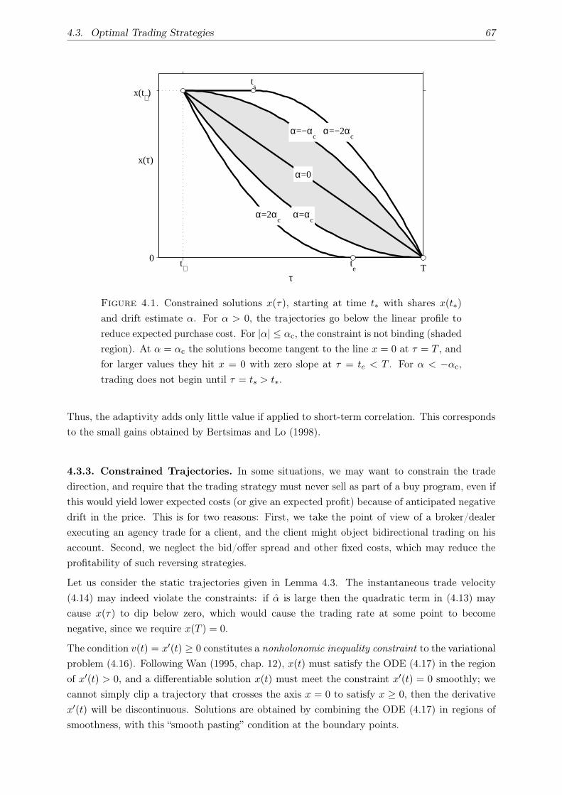
4.3. Optimal Trading Strategies 67
T0
α=−αc
α=αc
α=0
ts
te
α=−2αc
α=2αc
x(τ)
τt∗
x(t∗)
Figure 4.1. Constrained solutions x(τ), starting at time t∗ with shares x(t∗)
and drift estimate α. For α > 0, the trajectories go below the linear profile to
reduce expected purchase cost. For |α| ≤ αc, the constraint is not binding (shaded
region). At α = αc the solutions become tangent to the line x = 0 at τ = T , and
for larger values they hit x = 0 with zero slope at τ = te < T . For α < −αc,
trading does not begin until τ = ts > t∗.
Thus, the adaptivity adds only little value if applied to short-term correlation. This corresponds
to the small gains obtained by Bertsimas and Lo (1998).
4.3.3. Constrained Trajectories. In some situations, we may want to constrain the trade
direction, and require that the trading strategy must never sell as part of a buy program, even if
this would yield lower expected costs (or give an expected profit) because of anticipated negative
drift in the price. This is for two reasons: First, we take the point of view of a broker/dealer
executing an agency trade for a client, and the client might object bidirectional trading on his
account. Second, we neglect the bid/offer spread and other fixed costs, which may reduce the
profitability of such reversing strategies.
Let us consider the static trajectories given in Lemma 4.3. The instantaneous trade velocity
(4.14) may indeed violate the constraints: if α is large then the quadratic term in (4.13) may
cause x(τ) to dip below zero, which would cause the trading rate at some point to become
negative, since we require x(T ) = 0.
The condition v(t) = x′(t) ≥ 0 constitutes a nonholonomic inequality constraint to the variational
problem (4.16). Following Wan (1995, chap. 12), x(t) must satisfy the ODE (4.17) in the region
of x′(t) > 0, and a differentiable solution x(t) must meet the constraint x′(t) = 0 smoothly; we
cannot simply clip a trajectory that crosses the axis x = 0 to satisfy x ≥ 0, then the derivative
x′(t) will be discontinuous. Solutions are obtained by combining the ODE (4.17) in regions of
smoothness, with this “smooth pasting” condition at the boundary points.

68 Chapter 4. Bayesian Adaptive Trading with Price Appreciation
From (4.18) we see that there is in fact a critical drift value
αc
(x(t∗), T − t∗
)=
4η x(t∗)
(T − t∗)2.
For |α| ≤ αc, the trade rate v(τ) = −x′(τ), (4.18), of the trajectory (4.13) is positive for all
t∗ ≤ τ ≤ T , and the constraint v(τ) ≥ 0 never becomes binding.
For high negative drift α < −αc the unconstrained trajectory (4.13) would increase over x(t∗)
right after its start at t∗, i.e. the strategy short-sells in the beginning in order to capture
additional profit by buying back those extra shares later for lower prices; on the other hand, the
constrained trajectory does not start buying shares until some starting time ts > t∗. As already
mentioned, by the “smooth pasting” condition the trajectory has to start trading at ts with zero
slope v(ts) = 0.
Conversely, for high positive drift α > αc the unconstrained trajectory dips below zero in the
course of the trading in order to sell those additional shares again at the end of the day; contrary,
the constrained trajectory stops trading at a shortened end time te. Again, the trajectory has
to meet te with zero slope v(te) = 0.
The times ts and te are determined by the “smooth pasting” condition. The shortened end time
te is determined so that x′(te) = x(te) = 0, and is found as
te = t∗ +
√4η x(t∗)
α.
Note that since α > αc = 4ηx(t∗)/(T − t∗)2, we always have te < T .
The deferred start time ts is determined so that x′(ts) = 0 and x(ts) = x(t∗) and given by
ts = T −√
4η x(t∗)
−α.
Note that since α < −αc = −4ηx(t∗)/(T − t∗)2, we always have ts > t∗.
Figure 4.1 illustrates these solutions. The overall instantaneous trade rate at time 0 ≤ t∗ ≤ T of
a constrained optimal statc trajectory x(τ) | t∗ ≤ τ ≤ T specified at t∗ may be summarized as
v(t∗) =
0, α < −αc
x(t∗)
T − t∗+
α
4η
(T − t∗
), |α| < αc
x(t∗)
te − t∗+
α
4η
(te − t∗
)=√
αx(t∗)/η, α > αc
(4.30)
where α = α(t∗, S(t∗)
)is the best drift estimate at time t∗ given by Lemma 4.1.
From this discussion about the constrained static trajectories, it is conceivable that the optimal
adaptive constrained strategy is – similarly to the unconstrained case in Theorem 4.4 – obtained
by trading with the instantaneous trade rate (4.30) at every 0 ≤ t∗ ≤ T using the current best
drift estimate α = E [α | t∗, s(t∗)] at each moment. The dynamic programming approach to prove
the optimality of this strategy is still possible in principle, and leads to
0 = Jt +1
2σ2 Jss + α Js + min
v≥0
((s Jy − Jx
)v + ηJy v2
), (4.31)
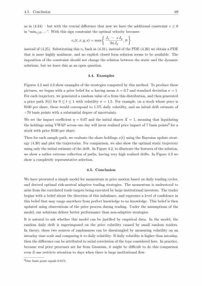
4.5. Conclusion 69
as in (4.24) – but with the crucial difference that now we have the additional constraint v ≥ 0
in “minv≥0 . . . ”. With this sign constraint the optimal velocity becomes
v∗(t, x, y, s) = max
Jx − s Jy
2η Jy, 0
instead of (4.25). Substituting this v∗ back in (4.31), instead of the PDE (4.26) we obtain a PDE
that is more highly nonlinear, and no explicit closed form solution seems to be available. The
imposition of the constraint should not change the relation between the static and the dynamic
solutions, but we leave this as an open question.
4.4. Examples
Figures 4.2 and 4.3 show examples of the strategies computed by this method. To produce these
pictures, we began with a prior belief for α having mean α = 0.7 and standard deviation ν = 1.
For each trajectory, we generated a random value of α from this distribution, and then generated
a price path S(t) for 0 ≤ t ≤ 1 with volatility σ = 1.5. For example, on a stock whose price is
$100 per share, these would correspond to 1.5% daily volatility, and an initial drift estimate of
+70 basis points with a substantial degree of uncertainty.
We set the impact coefficient η = 0.07 and the initial shares X = 1, meaning that liquidating
the holdings using VWAP across one day will incur realized price impact of 7 basis points2 for a
stock with price $100 per share.
Then for each sample path, we evaluate the share holdings x(t) using the Bayesian update strat-
egy (4.30) and plot the trajectories. For comparison, we also show the optimal static trajectory
using only the initial estimate of the drift. In Figure 4.2, to illustrate the features of the solution,
we show a rather extreme collection of paths, having very high realized drifts. In Figure 4.3 we
show a completely representative selection.
4.5. Conclusion
We have presented a simple model for momentum in price motion based on daily trading cycles,
and derived optimal risk-neutral adaptive trading strategies. The momentum is understood to
arise from the correlated trade targets being executed by large institutional investors. The trader
begins with a belief about the direction of this imbalance, and expresses a level of confidence in
this belief that may range anywhere from perfect knowledge to no knowledge. This belief is then
updated using observations of the price process during trading. Under the assumptions of the
model, our solutions deliver better performance than non-adaptive strategies.
It is natural to ask whether this model can be justified by empirical data. In the model, the
random daily drift is superimposed on the price volatility caused by small random traders.
In theory, these two sources of randomness can be disentangled by measuring volatility on an
intraday time scale and comparing it to daily volatility. If daily volatility is higher than intraday,
then the difference can be attributed to serial correlation of the type considered here. In practice,
because real price processes are far from Gaussian, it might be difficult to do this comparison
even if one restricts attention to days when there is large institutional flow.
2One basis point equals 0.01%.
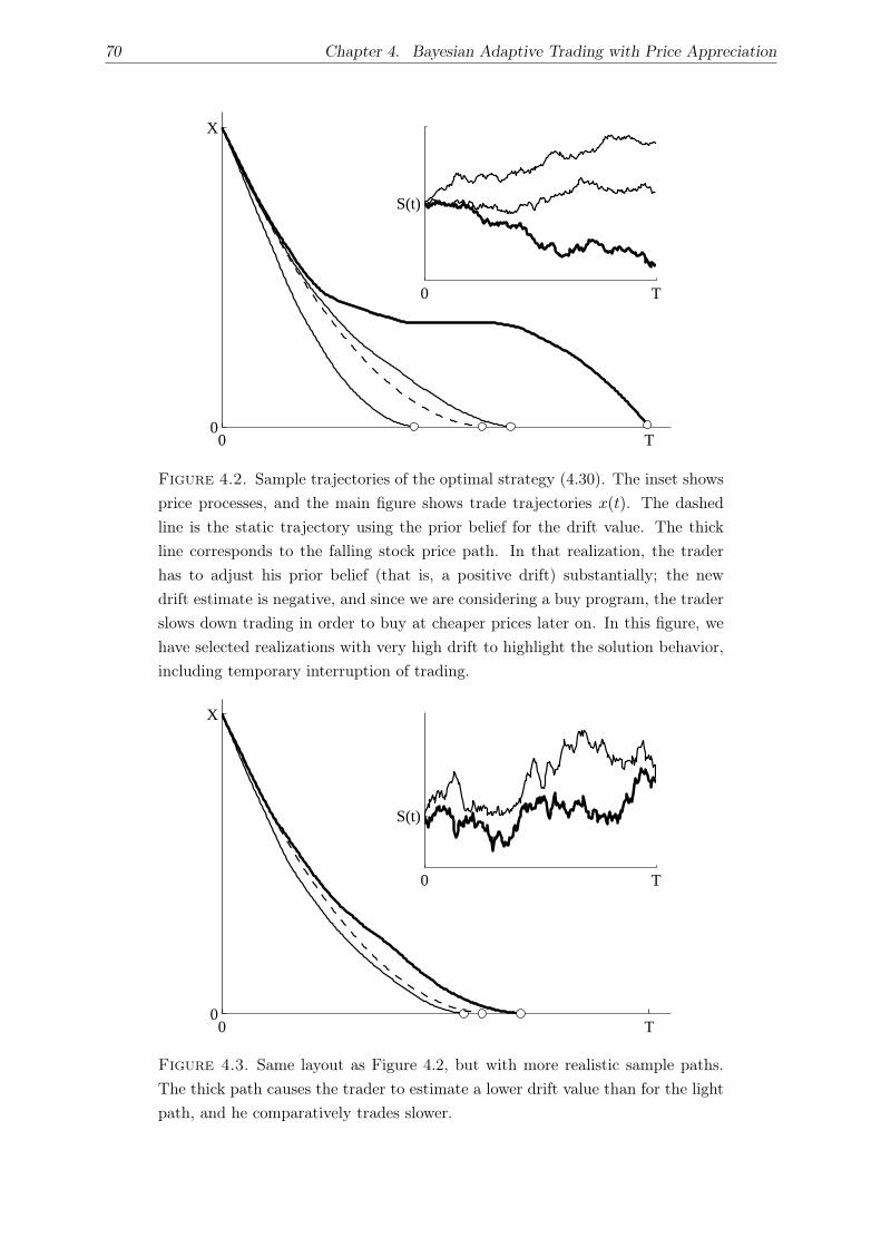
70 Chapter 4. Bayesian Adaptive Trading with Price Appreciation
0 T0
X
0 T
S(t)
Figure 4.2. Sample trajectories of the optimal strategy (4.30). The inset shows
price processes, and the main figure shows trade trajectories x(t). The dashed
line is the static trajectory using the prior belief for the drift value. The thick
line corresponds to the falling stock price path. In that realization, the trader
has to adjust his prior belief (that is, a positive drift) substantially; the new
drift estimate is negative, and since we are considering a buy program, the trader
slows down trading in order to buy at cheaper prices later on. In this figure, we
have selected realizations with very high drift to highlight the solution behavior,
including temporary interruption of trading.
0 T0
X
0 T
S(t)
Figure 4.3. Same layout as Figure 4.2, but with more realistic sample paths.
The thick path causes the trader to estimate a lower drift value than for the light
path, and he comparatively trades slower.

CHAPTER 5
Multiperiod Portfolio Optimization
In this chapter we show how the dynamic programming principle introduced in Chapter 3 can
be applied to solve the discrete-time multiperiod mean-variance portfolio problem. Our solution
coincides with the optimal strategy given by Li and Ng (2000).
5.1. Introduction
Research on portfolio theory was pioneered in the 1950s with the seminal work of Markowitz
(1952, 1959) on mean-variance efficient portfolios for a single period investment. While it is
natural to extend Markowitz’s work to multiperiod settings, difficulties arise from the definition
of the mean-variance objective E [X] − λ Var [X], which does not allow a direct application of
the dynamic programming principle (Bellman, 1957) due to the square of the expectation in the
variance term.
Work on multiperiod and continuous-time formulations of portfolio selection took a different ap-
proach and employed expected utility criteria (von Neumann and Morgenstern, 1953). Here, the
expected terminal wealth E [u(wT )] for a utility function u(·) is optimized, see for instance Mossin
(1968) and Samuelson (1969). Typical choices for u(·) are logarithmic, exponential, power or
quadratic functions. One of the most important breakthroughs in this area is due to Merton
(1969). Using Ito’s lemma and Bellman’s dynamic programming principle, he solved the problem
of optimal consumption and investment in continuous-time where the prices of the risky assets
follow diffusion processes and was able to derive closed-form optimal dynamic portfolio strategies
for some particular cases of utility functions u(·).In the original mean-variance formulation, Dantzig and Infanger (1993) show how multiperiod
portfolio problems can be efficiently solved as multistage stochastic linear programs, using sce-
nario generation and decomposition techniques. However, no analytical closed-form solution is
obtained.
In a rather influential paper, Li and Ng (2000) give a closed-form solution for the classical mean-
variance problem in discrete time. They introduce an embedding of the original mean-variance
problem into a tractable auxiliary problem with a utility function of quadratic type. Their
embedding technique provides a general framework of stochastic linear-quadratic (LQ) optimal
control in discrete time. Zhou and Li (2000) generalize this theory to continuous-time settings,
and also obtain a closed-form solution for the efficient frontier. In fact, prior to this work White
(1998) studied a similar approach to characterizes mean-variance efficient solution sets by a
parametric solution sets of first and second moment.
The embedding technique of Li and Ng (2000) and Zhou and Li (2000) set off a series of papers
on dynamic mean-variance optimization. Lim and Zhou (2002) consider stock price processes
71
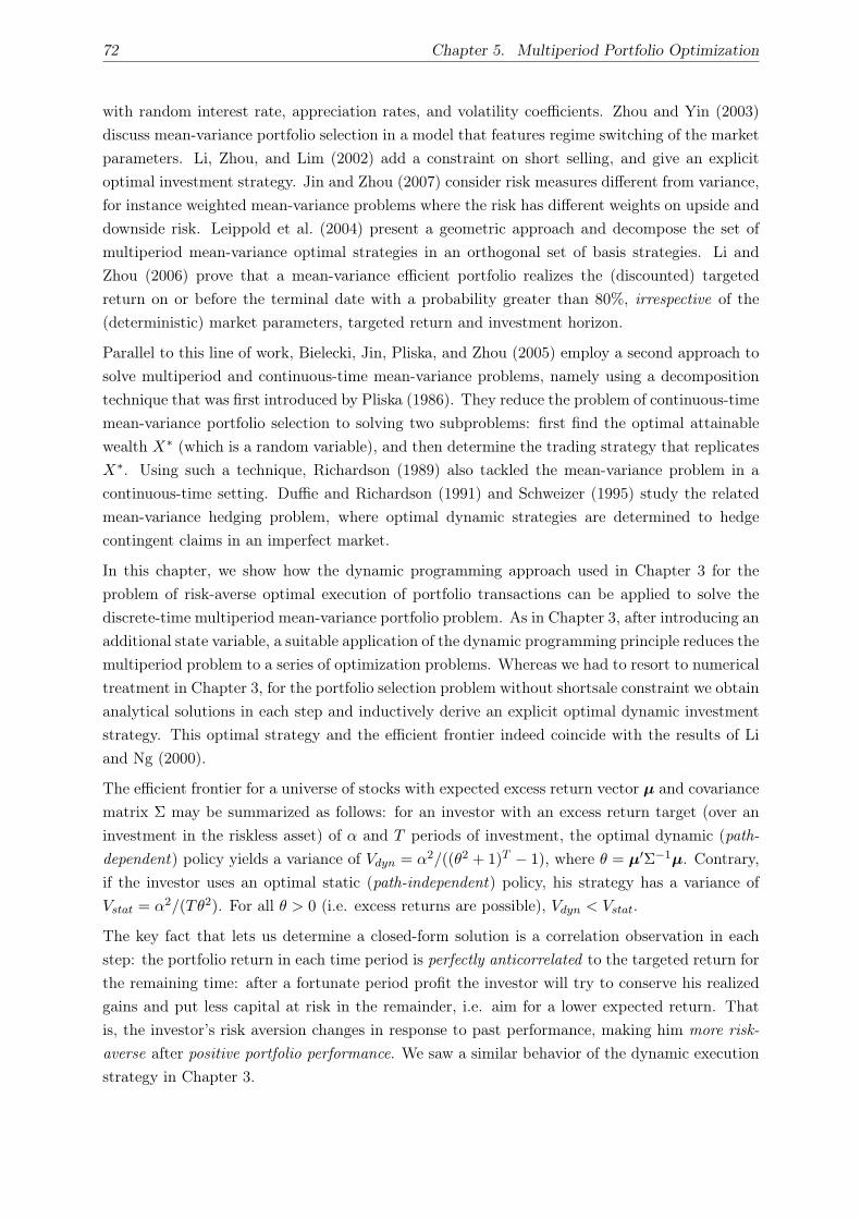
72 Chapter 5. Multiperiod Portfolio Optimization
with random interest rate, appreciation rates, and volatility coefficients. Zhou and Yin (2003)
discuss mean-variance portfolio selection in a model that features regime switching of the market
parameters. Li, Zhou, and Lim (2002) add a constraint on short selling, and give an explicit
optimal investment strategy. Jin and Zhou (2007) consider risk measures different from variance,
for instance weighted mean-variance problems where the risk has different weights on upside and
downside risk. Leippold et al. (2004) present a geometric approach and decompose the set of
multiperiod mean-variance optimal strategies in an orthogonal set of basis strategies. Li and
Zhou (2006) prove that a mean-variance efficient portfolio realizes the (discounted) targeted
return on or before the terminal date with a probability greater than 80%, irrespective of the
(deterministic) market parameters, targeted return and investment horizon.
Parallel to this line of work, Bielecki, Jin, Pliska, and Zhou (2005) employ a second approach to
solve multiperiod and continuous-time mean-variance problems, namely using a decomposition
technique that was first introduced by Pliska (1986). They reduce the problem of continuous-time
mean-variance portfolio selection to solving two subproblems: first find the optimal attainable
wealth X∗ (which is a random variable), and then determine the trading strategy that replicates
X∗. Using such a technique, Richardson (1989) also tackled the mean-variance problem in a
continuous-time setting. Duffie and Richardson (1991) and Schweizer (1995) study the related
mean-variance hedging problem, where optimal dynamic strategies are determined to hedge
contingent claims in an imperfect market.
In this chapter, we show how the dynamic programming approach used in Chapter 3 for the
problem of risk-averse optimal execution of portfolio transactions can be applied to solve the
discrete-time multiperiod mean-variance portfolio problem. As in Chapter 3, after introducing an
additional state variable, a suitable application of the dynamic programming principle reduces the
multiperiod problem to a series of optimization problems. Whereas we had to resort to numerical
treatment in Chapter 3, for the portfolio selection problem without shortsale constraint we obtain
analytical solutions in each step and inductively derive an explicit optimal dynamic investment
strategy. This optimal strategy and the efficient frontier indeed coincide with the results of Li
and Ng (2000).
The efficient frontier for a universe of stocks with expected excess return vector µ and covariance
matrix Σ may be summarized as follows: for an investor with an excess return target (over an
investment in the riskless asset) of α and T periods of investment, the optimal dynamic (path-
dependent) policy yields a variance of Vdyn = α2/((θ2 + 1)T − 1), where θ = µ′Σ−1
µ. Contrary,
if the investor uses an optimal static (path-independent) policy, his strategy has a variance of
Vstat = α2/(Tθ2). For all θ > 0 (i.e. excess returns are possible), Vdyn < Vstat.
The key fact that lets us determine a closed-form solution is a correlation observation in each
step: the portfolio return in each time period is perfectly anticorrelated to the targeted return for
the remaining time: after a fortunate period profit the investor will try to conserve his realized
gains and put less capital at risk in the remainder, i.e. aim for a lower expected return. That
is, the investor’s risk aversion changes in response to past performance, making him more risk-
averse after positive portfolio performance. We saw a similar behavior of the dynamic execution
strategy in Chapter 3.

5.2. Problem Formulation 73
This change in risk-aversion of the optimal multiperiod investment strategy is very apparent in
the direct dynamic programming approach that we propose. Hence, we hope that our technique
contributes to the understanding of the behavior of mean-variance optimal dynamic strategies
for multiperiod problems.
As it is well known, mean-variance based preference criteria have received theoretical criti-
cism (see for instance Maccheroni et al., 2004). However, mean-variance portfolio optimization
retains great practical importance due to its clear intuitive meaning. Compared to utility based
criteria, mean-variance optimization has the advantage that no assumptions on the investor’s
utility function are needed. From the perspective of an investment company, who does not know
about its clients’ utility or about their other investment activities, one solution is to offer the
efficient frontier of mean-variance optimal portfolio strategies, and let the clients pick according
to their needs. Another advantage is that the trade-off between risk and return is explicitly given,
and not only implicitly contained in the utility function. The relationship between mean-variance
optimization and the expected utility framework is discussed, for instance, by Kroll et al. (1984)
and Markowitz (1991).
The remainder of this chapter is organized as follows. We formulate the discrete-time multiperiod
mean-variance portfolio selection problem in Section 5.2. In Section 5.3, we show how mean-
variance optimization becomes amenable to dynamic programming by a suitable choice of the
value function. Using this framework, we derive the explicit solution for the multiperiod portfolio
problem in Section 5.4.
5.2. Problem Formulation
An investor has an initial wealth of w0, and wants to invest across T periods with no consumption,
generating intermediate wealth w1, . . . , wT . His only concern is to maximize the final wealth wT ,
while also minimizing its riskiness (drawdowns, etc, are of no concern).
There are n risky assets with prices St = (S1t , . . . , Sn
t )′ and one riskless asset with price S0t
(all vectors are column vectors, and ′ denotes transpose). The riskless asset has a fixed return
r = S0t+1/S0
t > 0. The excess returns of the risky assets at time t are et = (ξ1t , . . . , ξn
t )′, with
eit =
Sit+1
Sit
− r .
The excess return vectors e0, . . . , eT−1 are i.i.d. random variables with known mean vector µ =
E [et] and covariance matrix Σ = E [(et − µ)(et − µ)′]. Since we assume the returns et identically
distributed, µ and Σ are time-independent. In principle, the framework in this chapter also
works for non-identically distributed excess returns et as well, but closed-form solutions of the
final efficient frontier and optimal strategies will be much more difficult to obtain (if at all).
At least one component of µ must be nonzero so that excess expected profits are possible—the
sign is not important since we allow arbitrary short sales—and Σ must be strictly positive definite
so that there are no non-risky combinations of the risky assets.
We denote by Ω ⊂ Rn the set of possible values of each et, and we make no assumptions about
the structure of Ω. The returns may be multivariate normal, a multinomial tree taking m distinct

74 Chapter 5. Multiperiod Portfolio Optimization
values at each step (m > n so that Σ may be positive definite), or anything else. All we need
are the mean and variance as stated.
Let It be the σ-algebra generated by e0, . . . , et−1, for t = 0, . . . , T . For t = 0, . . . , T − 1, Itis the information available to the investor before he makes his investment at time t; since w0
is nonrandom, It also includes the wealth w0, . . . , wt. IT is the information set after the end of
the last investment period, when he simply collects the final value wT .
An investment plan for the t-th period is an It-measurable vector yt = (y1t , . . . , y
nt )′, where
yit is the amount invested in the i-th risky asset. The amount invested in the riskless asset is
y0t = wt −
∑ni=1 yi
t, and the system dynamics can be summarized in the discrete time stochastic
system
wt+1 = f(wt,yt, et
)(5.1)
for t = 0, 1, . . . , T − 1, with
f(wt,yt, et) = rwt + e′tyt . (5.2)
The series of these investment decisions (y0, . . . ,yT−1) constitutes a nonanticipating portfolio
policy π. We let A0 be the set of all such policies; we do not consider portfolio constraints other
than mean and variance limits, but such restrictions could easily be included in the definition
of A0. Also, our overall approach can be extended to general systems with structure (5.1),
independently of the specific form (5.2).
The problem of the mean-variance investor can be stated in any one of the following three forms:
P1(α) Minimize the variance of wealth for a given level of expected wealth:
minπ∈A0
Var [wT ] such that E [wT ] = α .
P2(σ) Maximize the expected value of wealth for a given level of variance:
maxπ∈A0
E [wT ] such that Var [wT ] = σ2 .
P3(λ) Maximize a combination of expectation and variance for a given risk aversion coefficient
λ ≥ 0:
maxπ∈A0
(E [wT ]− λ Var [wT ]
).
These formulations are essentially equivalent (Li and Ng, 2000). In practice one might prefer to
meet or exceed a return target, or to incur not more than a maximum variance, rather than the
equality constraints as stated above. For technical reasons in Section 5.4 we prefer the equality
targets.
In stating P1–P3, it is implicit that expectation and variance are evaluated at t = 0, before any
information is revealed. The portfolio policy π lays down a rule for the entire investment process,
for every possible series of “states of nature” until time T (all possible stock price paths). We can
understand this as programing a computer at time t = 0, in order to optimize the expectation
and variance of final wealth wt measured at time t = 0. This program might contradict the risk-
reward preference of the “future self” of the investor at some later time t = k: if the investor were
to re-program the computer at t = k in order to optimize mean and variance of wT – measured
at time t = k – according to his risk-reward preference, he might want to do differently as he
sees gains or losses made between t = 0 and t = k as sunk cost.
5.3. Dynamic Programming 75
An example of this type of optimization in the financial industry is trading a portfolio on behalf
of a client. At the time when the client entrusts his bank (or other institutional fund manager)
with his money, he communicates his risk-reward preference. He is then only given reports of
the portfolio performance at the end of the year, leaving the daily trading activities to the bank.
Consequently, at the beginning of each year the bank has to determine a portfolio strategy that
optimizes the client’s wealth at the end of the year, since that is how the bank is evaluated by
the client.
5.3. Dynamic Programming
Of the three formulations above, the third P3(λ) is the most general, often appearing as a
Lagrange multiplier approach to either of the first two. It is also appealing because it is strongly
reminiscent of a utility function u(wT ), and it is known that multi-step problems involving
utility maximization max E [u(wT )] can be solved by dynamic programming, reducing them to a
sequence of single-period problems.
But despite this apparent similarity, problem P3(λ) cannot be used directly as a utility func-
tion on the stochastic system (5.1,5.2), since the variance Var [wT ] = E[w2
T
]− E [wT ]2 in-
volves the square of the expectation, and hence does not fit into the framework of expected
utility maximization. The dynamic programming approach relies on the “smoothing property”
E [E [u(wT ) | Is] | It] = E [u(wT ) | It] for s > t, which does not hold for the variance term
Var [u(wT )]. Zhou and Li (2000) overcome this obstacle by using an embedding of E [wT ] −λ Var [wT ] into a family of truely quadratic utility functions E
[ρwT − λw2
T
]with an additional
parameter ρ ∈ R and relating the solution set for (λ, ρ) to the original problem P3(λ). Unfor-
tunately, the introduction of the additional parameter ρ greatly complicates the problem and
makes it hard to obtain explicit solutions.
As in Chapter 3, we now show how we can apply dynamic programming directly to the multi-
period mean-variance optimization problem, with a suitable choice of the value function. In the
following, we will solve the problem in formulation P1(α), and derive the solutions for P2(σ) and
P3(λ) from that. In fact, the approach could as well adopted to solve instead P2(σ) directly.
Recall that yt is the investor’s investment decision at time t = 0, . . . , T − 1, and that the excess
return of this investment from t to t + 1 is e′tyt. Let
gt(yt, et) = rT−t−1e′tyt (5.3)
be the eventual value at time T of this excess gain, reinvested for the remaining periods at the
riskless rate. Note that
wT − rT−twt =T−1∑
s=t
gs(ys, es) for t = 0, 1, . . . , T − 1 .
For t = 0, . . . , T − 1, let At be the set of all nonanticipating portfolio policies that start at time
t: the investor makes his first investment at t, and the last at T − 1. Let Gt(wt, α) ⊂ At be the
set of all non-anticipating portfolio policies that start at time t with wealth wt, for which the
expected excess gain of final wealth over the riskless investment is exactly α:
Gt(wt, α) =
π ∈ At
∣∣ E[wT − rT−twt
∣∣ It]
= α
. (5.4)
76 Chapter 5. Multiperiod Portfolio Optimization
It is easy to see that Gt is nonempty for all wt and α, for nonzero µ and with no investment
limits; for example, the constant investment yt = · · · = yT−1 = y yields an expected excess gain
of µ′y · (1 + r + · · ·+ rT−t−1), which may take any desired value α by choice of y.
For t = 0, . . . , T − 1, consider the value function
Jt(wt, α) = minπ∈Gt(wt,α)
Var [wT | It] = minπ∈Gt(wt,α)
Var
[T−1∑
s=t
gs(ys, es)
∣∣∣∣∣ It]
, (5.5)
which is the minimum variance of final wealth achievable by an investment policy for t, . . . , T −1
such that the expected final excess gain is α, starting with current wealth wt. The solution to
problem P1(α) is J0
(w0, α− rT w0
), together with the corresponding optimal policy π∗ ∈ A0.
As in Chapter 3 we use the law of total variance (see Lemma 3.1), the counterpart to the
smoothing property of the expectation operator mentioned above. In particular, for s = t + 1,
Var [wT | It] = Var [E [wT | It+1] | It] + E [Var [wT | It+1] | It] . (5.6)
In this expression, E [wT | It+1] is still uncertain at time t, since it depends on the outcome of the
period return et. The first term can thus be thought of the risk resulting from the uncertainty
between t and t + 1.
Var [wT | It+1] is the risk that we will face in the remaining periods from t+1 and T . The second
term is therefore the mean risk for the remainder after the next period.
As in Chapter 3, the key idea is that the expected gain for the remaining periods between t + 1
and T does not have to be the same for all possible outcomes of et. At time t, we specify target
expected returns for the remaining time, depending on the portfolio return in the period to come.
Thus, we make our investment strategy for t + 2, . . . , T dependent on the performance of our
portfolio over the next period. For instance, we might plan that after a fortunate windfall profit
we will conserve the realized gain and be content with less expected return for the remainder,
putting less capital at risk. Crucially, we choose this rule to optimize mean and variance measured
at the current time t; it is this that makes dynamic programming possible.
We specify E [wT | It+1] in terms of a It+1-measurable random variable
zt = E [wT | It+1] − rT−t−1wt+1 .
The value of zt may depend on et (asset prices and wealth at t+1) in addition to w0, . . . , wt and
e0, . . . , et−1. Thus, zt may be interpreted as a function Ω → R, measurable in the probability
measure of et. Let L be the set of all such functions.
The function zt is determined at time t, and specifies for each possible outcome of et what excess
return target we will set for the remaining periods. Recall that yt is It-measurable and hence
may not depend on et. Whereas the dimension of yt is the number of assets n, the dimension of
zt is the cardinality of Ω, which may be a finite number m or infinity.
In terms of zt and the dynamics (5.1,5.2), we have
E [wT | It+1] = rT−t−1wt+1 + zt = rT−twt + rT−t−1e′tyt + zt (5.7)
and, assuming that we make optimal decisions from t + 1 to T ,
Var [wT | It+1] = Jt+1(wt+1, zt) = Jt+1
(rwt + e′tyt, zt
). (5.8)

5.4. Explicit Solution 77
Not all functions zt are compatible with our current excess return target α. Using (5.7), we may
write the eventual expected excess return as
E[wT − rT−twt
∣∣ It]
= rT−t−1µ′yt + E [zt] .
Thus the set of (y, z) pairs that yield the desired final excess profit of α, as required by (5.4), is
Gt(α) =
y ∈ Rn, z ∈ L∣∣∣ rT−t−1
µ′y + E [z] = α
.
This is simply a linear condition on the pair (y, z): if we choose an investment y that yields a
low expected profit this period, then we must compensate by setting higher targets z for the
remaining periods. The above expressions are valid for t = 0, . . . , T − 2; for t = T − 1, it is easy
to see that the same expressions hold without the terms including z.
Suppose we have already determined Jt+1(wt+1, α). By the dynamic programming principle with
(5.6,5.7,5.8), we obtain
Jt(wt, α) = minGt(w,α)
Var[wT − rT−twt
∣∣ It]
= min(y,z)∈Gt(α)
Var
[rT−t−1e′ty + z
]+ E
[Jt+1(rwt + e′ty, z)
] . (5.9)
In this expression, expectation and variance of e and z = z(e) are taken using the density of
e = et on its sample space Ω.
Equation (5.9) completely describes the dynamic program to find optimal Markovian policies for
P1(α).
As seen in Chapter 3, even for more complicated system dynamics f(·) than (5.2), a dynamic
program for multiperiod mean-variance optimization problems in discrete time can be derived.
For the portfolio transaction problem in Chapter 3, we had to resort to numerical treatment
to solve the dynamic program. Contrary, in the following we will show that for the portfolio
selection problem we can solve (5.9) analytically, and inductively derive a closed-form solution
for the value function at time t = 0.
5.4. Explicit Solution
Before we solve the optimization problem (5.9) in the backwards step, we need to find the
solution for the single-period problem JT−1(w, α) first, which is easily obtained as the solution
of a constrained quadratic program:
Lemma 5.1.
JT−1(w, α) = α2/θ2 , θ2 = µ′Σ−1
µ . (5.10)
Proof. For current wealth w and required expected excess gain α, the single-period mean-
variance problem reads
miny∈Rn
y′Σy s.t. µ′y = α . (5.11)
The solution is easily found as y = αΣ−1µ/θ2, which yields the t = T − 1 value function
JT−1(w, α) = α2/θ2.

78 Chapter 5. Multiperiod Portfolio Optimization
Now we are ready to derive the explicit solution of the portfolio selection problem by the dynamic
program stated in Sect. 5.3.
Lemma 5.2. The optimal investment decision at time t for a mean-variance investor with current
wealth wt = w, who is optimizing P1(α + rT−twt), i.e.
min Var [wT | It] s.t. E[wT − rT−twt
∣∣ It]
= α ,
is the control (yt, zt) given by
y∗t =
α
rτ−1
1 + θ2τ−1
θ2τ
Σ−1µ (5.12)
z∗t = αθ2τ−1
θ2τ
(1− µ
′Σ−1(et − µ))
(5.13)
with τ = T − t and
θ 2τ = (θ2 + 1)τ − 1 for 0 ≤ τ ≤ T , (5.14)
with θ2 = µ′Σ−1
µ. Here, y∗t is the optimal investment vector and z∗t gives the planned expected
gain the investor commits himself for the remaining periods t + 1, . . . , T as a function of the
realized outcome of the return et over the period to come. The value function (5.5) is
Jt(wt, α) = inf
Var [wT | It]∣∣∣ E[wT − rT−twt
∣∣ It]
= α
=α2
θ 2τ
. (5.15)
Proof. We prove by induction. Since θ0 = 0 and θ1 = θ, Lemma 5.1 proves the result for
t = T − 1. For 0 ≤ t ≤ T − 2, assume that Jt+1(w, α) = α2/θ2τ−1, and then the dynamic
programming step (5.9) is
Jt(w, α) = infy,z
V (y, z)
∣∣∣ E(y, z) = α
(5.16)
with
E(y, z) = rτ−1µ′y + E [z]
V (y, z) = Var[rτ−1e′y + z
]+
1
θ2τ−1
E[z2]
.
Here and in the following we use e = et instead of et to shorten notation.
Our first observation is that, since
Var[rτ−1e′y + z
]= Var
[rτ−1e′y
]+ Var [z] + 2rτ−1 Cov
[e′y, z
],
we can generally reduce V (y, z) by introducing negative correlation between e′y and z, where
correlation between two random variables X and Y with positive variance is the standard
ρ(X, Y ) = Cov [X, Y ] /√
Var [X] Var [Y ]. In fact, we now show that in the optimal solution,
these two terms have precisely minimal correlation ρ(e′y, z) = −1.
To see that, suppose ρ(e′y∗, z∗
)> −1. Consider the control (y∗, z) with z = a e′y∗ + b, where
a = −√
Var [z∗] / Var [e′y∗] and b = E [z∗] − a E [e′y∗]. Then z∗ and z have identical first and
second moments, but ρ(e′y∗, z) = −1 < ρ(e′y∗, z∗) implies Cov [e′y∗, z] < Cov [e′y∗, z∗], and
thus the control (y∗, z) yields a lower value of V for the same E. This correlation observation is
the key fact that lets us determine the optimal solution independently of the structure of Ω.

5.4. Explicit Solution 79
Thus, up to a set of zero measure, we must have
z = arτ−1(e− µ)′y + b , (5.17)
for some a < 0 and b ∈ R (note that µ′y is a constant). Then
E [z] = b
E[z2]
= b2 + a2r2(τ−1)y′Σy
Var[rτ−1e′y + z
]= (a + 1)2r2(τ−1)y′Σy ,
and we may write E(y, z) and V (y, z) in terms of y, a, and b as
E(y, a, b) = rτ−1µ′y + b , (5.18)
V (y, a, b) =b2
θ 2τ−1
+
((a + 1)2 +
a2
θ 2τ−1
)r2(τ−1)y′Σy . (5.19)
Instead of solving (5.16) directly, we optimize the trade-off function
H(w, λ) = supy∈Rn,a<0,b∈R
L(y, a, b, λ) for λ > 0 , (5.20)
with
L(y, a, b, λ) = E(y, a, b)− λV (y, a, b) . (5.21)
Since L(y, a, b, λ) is a convex quadratic function in (y, a, b), there exists a unique optimum, which
we can find by first-order conditions.
The first-order conditions ∂L/∂a = 0 and ∂L/∂b = 0 immediately yield
a∗ = − θ2τ−1
1 + θ2τ−1
and b∗ =θ2τ−1
2λ.
Plugging a∗ and b∗ into the first-order condition for y, we obtain
y∗(λ) =1 + θ 2
τ−1
2λrτ−1Σ−1
µ ,
then
z∗(λ) =θ 2τ−1
2λ
(1− µ
′Σ−1(e− µ))
and finally
E∗(λ) =θ 2τ−1(θ
2 + 1) + θ2
2λ=
θ 2τ
2λ
V ∗(λ) =θ 2τ−1(θ
2 + 1) + θ2
4λ2=
θ2τ
4λ2,
where we use the definition (5.14) of θt. Solving E∗(λ) = α gives λ = θ 2τ /2α, and we obtain
(5.12,5.13) by substituting λ above, and finally
Jt(w, α) = V ∗(λ) = α2/θ2τ ,
which completes the inductive proof.

80 Chapter 5. Multiperiod Portfolio Optimization
We can give the optimal policy (y0, . . . ,yT−1) explicitly in terms of ei. Let
At =t−1∏
s=0
(1− µ
′Σ−1(es − µ))
(5.22)
(A0 = 1). Then
Theorem 5.3. For T ≥ 1, the adaptive solution to P1(α) is the mean-variance efficient frontier,
E = E [wT ] and V = Var [wT ],
E = α, V (α) =(α− rT w0
)2/θ2
T , (5.23)
and the optimal portfolio strategy (y0, . . . ,yT−1) in terms of ei is
yt =(α− rT w
) 1 + θ2T−t−1
rT−t−1θ2T
AtΣ−1
µ , (5.24)
with At from (5.22) and θT from (5.14).
Proof. Equation (5.23) follows directly from Lemma 5.2. By induction, we will now prove
yt =(α− rT w
) 1 + θ2T−t−1
rT−t−1θ2T
AtΣ−1
µ , (5.25)
zt =(α− rT w
) θ2T−t−1
θ2T
At+1 . (5.26)
For t = 0, (5.25, 5.26) follows from Lemma 5.2. Suppose (5.25, 5.26) hold at time t− 1. Then,
again by Lemma 5.2
yt = zt−1
1 + θ2T−t−1
rT−t−1θ2T−t
Σ−1µ
=(α− rT w
) θ2T−t
θ2T
At ·1 + θ2
T−t−1
rT−t−1θ2T−t
Σ−1µ
and
zt = zt−1θ2T−t−1
θ2T
(1− µ
′Σ−1(et − µ))
=(α− rT w
) θ2T−t
θ2T
At ·θ2T−t−1
θ2T−t
(1− µ
′Σ−1(et − µ))
,
completing the inductive proof.
From Theorem 5.3, we can easily derive the solutions for P2(σ) and P3(λ).
Corollary 5.4. Let T ≥ 1. Let θT and At defined by (5.14) and (5.22).
(i) The adaptive solution to P2(σ) is given by the mean-variance efficient frontier
(E(σ), σ2) |E(σ) = w0r
T + σθT and σ ≥ 0
.
(ii) The solution to P3(λ), i.e. the value of U(λ) = E [wT ] − λ − Var [wT ] under an optimal
adaptive strategy, is
U(λ) = w0rT + θ2
T /(4λ) .

5.4. Explicit Solution 81
Furthermore, the optimal portfolio strategy (y0, . . . ,yT−1) is given by
yt = γ · 1 + θ2T−t−1
rT−t−1θ2T
AtΣ−1
µ , (5.27)
where γ = θT σ in the case of P2(σ) and γ = θ2T /(2λ) in the case of P3(λ).
Proof. From (5.23), for given V (α∗) = σ2 we first obtain α∗ = wrT +θT σ. The optimal solution
for P2(σ) is then given by the optimal solution (5.24) for P1(α) with α = α∗ = wrT + θT σ.
For P3(λ), note that the optimal solution for maxπE [wT ] − λ Var [wT ] for given λ ≥ 0
can only lie on the E-V-frontier given by (5.23). Thus, it is equivalent to solve maxα≥0α −λ(α− w0r
T )2/θ2T , which is optimized by α∗ = θ2
T /(2λ) + w0rT with optimal value U(λ) =
w0rT + θ2
T /(4λ), and the optimal solution for P3(α) is given by the optimal solution for P1(α)
with α = α∗ = θ2T /(2λ) + w0r
T .
As can be seen from (5.24), similar to the well-known fund-separation theorem the proportions of
the assets in the risky part of the portfolio in an optimal adaptive investment policy are constant
throughout, given by Σ−1µ. What varies is the total amount invested in risky assets.
The expression for the mean-variance efficient frontier coincide with the expression given by Li
and Ng (2000). However, the optimal policy is specified differently. Li and Ng (2000) give the
optimal investment decision at time t as a function of the current wealth wt. In Theorem 5.3
and Corollary 5.4 the optimal investment decision is given as a function of the sequence of the
returns et.
We can also rewrite the optimal strategy as a function of the wealth process wt.
Theorem 5.5. Let α = α−w0rT be the expected excess return. The adaptive solution to P1(α),
given in Theorem 5.3, can be rewritten as a function of the wealth process wt as
ytr−t =
Σ−1µr
(θ2 + 1)
(α
1 + θ2T
θ2T
−(wtr
−t − w0
)). (5.28)
Proof. We prove by induction. By Theorem 5.3, we have
y0 = α1 + θ2
T−1
rT−1θ2T
Σ−1µ .
Since (1 + θ2T )/(1 + θ2) = 1 + θ2
T−1, this shows the base case t = 0.
For the inductive step, note that by Theorem 5.3,
yt+1 = α1 + θ2
T−t−2
rT−t−2θ2T
At
(1− µ
′Σ−1(et − µ))Σ−1
µ
= ytr
θ2 + 1
(1 + θ2 − µ
′Σ−1et
)= ytr
(1− µ
′Σ−1et
θ2 + 1
).
Hence, with the inductive hypothesis, we conclude
yt+1 − ytr = −ytre′tΣ
−1µ
1 + θ2
(5.28)= −rΣ−1
µe′tyt
θ2 + 1.
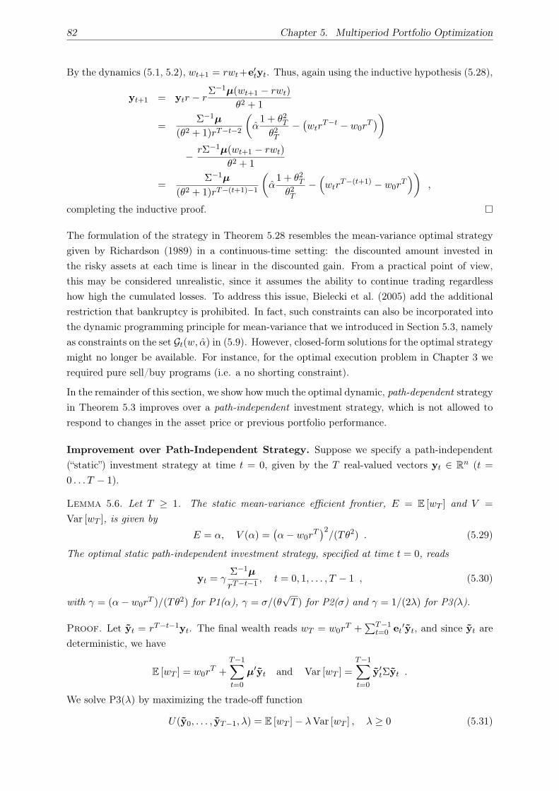
82 Chapter 5. Multiperiod Portfolio Optimization
By the dynamics (5.1, 5.2), wt+1 = rwt+e′tyt. Thus, again using the inductive hypothesis (5.28),
yt+1 = ytr − rΣ−1
µ(wt+1 − rwt)
θ2 + 1
=Σ−1
µ
(θ2 + 1)rT−t−2
(α
1 + θ2T
θ2T
−(wtr
T−t − w0rT))
− rΣ−1µ(wt+1 − rwt)
θ2 + 1
=Σ−1
µ
(θ2 + 1)rT−(t+1)−1
(α
1 + θ2T
θ2T
−(wtr
T−(t+1) − w0rT))
,
completing the inductive proof.
The formulation of the strategy in Theorem 5.28 resembles the mean-variance optimal strategy
given by Richardson (1989) in a continuous-time setting: the discounted amount invested in
the risky assets at each time is linear in the discounted gain. From a practical point of view,
this may be considered unrealistic, since it assumes the ability to continue trading regardless
how high the cumulated losses. To address this issue, Bielecki et al. (2005) add the additional
restriction that bankruptcy is prohibited. In fact, such constraints can also be incorporated into
the dynamic programming principle for mean-variance that we introduced in Section 5.3, namely
as constraints on the set Gt(w, α) in (5.9). However, closed-form solutions for the optimal strategy
might no longer be available. For instance, for the optimal execution problem in Chapter 3 we
required pure sell/buy programs (i.e. a no shorting constraint).
In the remainder of this section, we show how much the optimal dynamic, path-dependent strategy
in Theorem 5.3 improves over a path-independent investment strategy, which is not allowed to
respond to changes in the asset price or previous portfolio performance.
Improvement over Path-Independent Strategy. Suppose we specify a path-independent
(“static”) investment strategy at time t = 0, given by the T real-valued vectors yt ∈ Rn (t =
0 . . . T − 1).
Lemma 5.6. Let T ≥ 1. The static mean-variance efficient frontier, E = E [wT ] and V =
Var [wT ], is given by
E = α, V (α) =(α− w0r
T)2
/(Tθ2) . (5.29)
The optimal static path-independent investment strategy, specified at time t = 0, reads
yt = γΣ−1
µ
rT−t−1, t = 0, 1, . . . , T − 1 , (5.30)
with γ = (α− w0rT )/(Tθ2) for P1(α), γ = σ/(θ
√T ) for P2(σ) and γ = 1/(2λ) for P3(λ).
Proof. Let yt = rT−t−1yt. The final wealth reads wT = w0rT +
∑T−1t=0 et
′yt, and since yt are
deterministic, we have
E [wT ] = w0rT +
T−1∑
t=0
µ′yt and Var [wT ] =
T−1∑
t=0
y′tΣyt .
We solve P3(λ) by maximizing the trade-off function
U(y0, . . . , yT−1, λ) = E [wT ]− λ Var [wT ] , λ ≥ 0 (5.31)
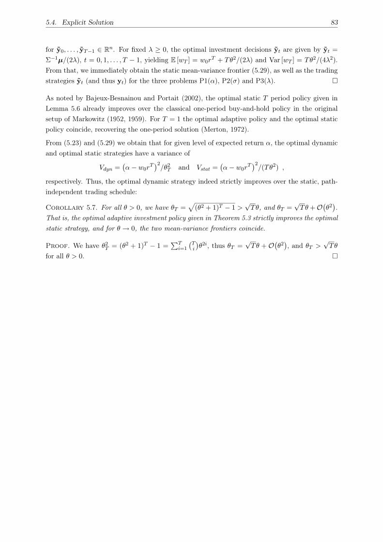
5.4. Explicit Solution 83
for y0, . . . , yT−1 ∈ Rn. For fixed λ ≥ 0, the optimal investment decisions yt are given by yt =
Σ−1µ/(2λ), t = 0, 1, . . . , T − 1, yielding E [wT ] = w0r
T + Tθ2/(2λ) and Var [wT ] = Tθ2/(4λ2).
From that, we immediately obtain the static mean-variance frontier (5.29), as well as the trading
strategies yt (and thus yt) for the three problems P1(α), P2(σ) and P3(λ).
As noted by Bajeux-Besnainou and Portait (2002), the optimal static T period policy given in
Lemma 5.6 already improves over the classical one-period buy-and-hold policy in the original
setup of Markowitz (1952, 1959). For T = 1 the optimal adaptive policy and the optimal static
policy coincide, recovering the one-period solution (Merton, 1972).
From (5.23) and (5.29) we obtain that for given level of expected return α, the optimal dynamic
and optimal static strategies have a variance of
Vdyn =(α− w0r
T)2
/θ2T and Vstat =
(α− w0r
T)2
/(Tθ2) ,
respectively. Thus, the optimal dynamic strategy indeed strictly improves over the static, path-
independent trading schedule:
Corollary 5.7. For all θ > 0, we have θT =√
(θ2 + 1)T − 1 >√
Tθ, and θT =√
Tθ +O(θ2).
That is, the optimal adaptive investment policy given in Theorem 5.3 strictly improves the optimal
static strategy, and for θ → 0, the two mean-variance frontiers coincide.
Proof. We have θ2T = (θ2 + 1)T − 1 =
∑Ti=1
(Ti
)θ2i, thus θT =
√Tθ + O
(θ2), and θT >
√Tθ
for all θ > 0.


CHAPTER 6
Optimal k-Search and Pricing of Lookback Options
In this chapter, we study the k-search problem, in which an online player is searching for the k
highest (respectively, lowest) prices in a series of price quotations which are sequentially revealed
to him. We analyze the problem using competitive analysis, and we give deterministic and
randomized algorithms as well as lower bounds for the competitive ratio. We also show the
usefulness of these algorithms to derive bounds for the price of “lookback options”.
6.1. Introduction
In this chapter, we consider the following online search problem: an online player wants to sell
(respectively, buy) k ≥ 1 units of an asset with the goal of maximizing his profit (minimizing
his cost). At time points i = 1, . . . , n, the player is presented a price quotation pi, and must
immediately decide whether or not to sell (buy) one unit of the asset for that price. The player
is required to complete the transaction by some point in time n. We ensure that by assuming
that if at time n− j he has still j units left to sell (respectively, buy), he is compelled to do so
in the remaining j periods. We shall refer to the profit maximization version (selling k units) as
k-max-search, and to the cost minimization version (purchasing k units) as k-min-search.
We shall make no modeling assumptions on the price path except that it has finite support, which
is known to the player. That is, the prices are chosen from the real interval I = x |m ≤ x ≤M,where 0 < m < M (see Figure 6.1). We define the fluctuation ratio ϕ = M/m. Let P =
⋃n≥k In
be the set of all price sequences of length at least k. Moreover, the length of the sequence is
known to the player at the beginning of the game.
0 5 10 15 20 2580
100
120
140
160
180
200
220
Figure 6.1. Example of a bounded price path with m = 100, ϕ = 2.
85

86 Chapter 6. Optimal k-Search and Pricing of Lookback Options
6.1.1. Online Algorithms and Competitive Analysis. In this section we briefly sketch the
concepts of online algorithms and competitive analysis. The reader is referred to the textbook
of Borodin and El-Yaniv (1998) for more details.
An online algorithm is an algorithm that processes its input piece-by-piece, without having the
entire input available from the start. Many problems in disciplines such as computer science,
economics or operations research are intrinsically online in that they require immediate decisions
to be made in real time (for instance, trading). From a broader perspective, online algorithms
fall into the field of decision-making in the absence of complete information.
Competitive analysis is a method for analyzing online algorithms, in which the performance of an
online algorithm is compared to the performance of an optimal offline algorithm that has access to
the entire input in advance. The optimal offline algorithm is in a sense hypothetical for an online
problem since it requires clairvoyant abilities and is thus not realizable. The competitive ratio of
an algorithm is understood as the worst-case ratio of its performance (measured by a problem
specific value) and the optimal offline algorithm’s performance. One imagines an “adversary” that
deliberately chooses difficult inputs in order to maximize this performance ratio. Competitive
analysis thus falls within the framework of worst-case analysis.
More precisely, let ALG be an online algorithm, and let OPT be the offline optimum algorithm
(which knows the entire input sequence in advance) for the same problem. In the case of k-search,
the input sequence is a price sequence σ, chosen by an adversary out of the set P of admissible
sequences. Let ALG(σ) and OPT(σ) denote the objective values of ALG and OPT when executed
on σ ∈ P. The competitive ratio of ALG is defined for maximization problems as
CR(ALG) = max
OPT(σ)
ALG(σ)
∣∣∣ σ ∈ P
,
and similarly, for minimization problems
CR(ALG) = max
ALG(σ)
OPT(σ)
∣∣∣ σ ∈ P
.
We say that ALG is c-competitive if it achieves a competitive ratio not larger than c. For ran-
domized algorithms, we substitute the expected objective value E [ALG] for ALG in the definitions
above.
The roots of competitive analysis lie in classical combinatorial optimization theory. Although
not named “competitive analysis”, Yao (1980) applied it to study how well online bin packing
algorithms perform. Later it was first explicitly advocated by Sleator and Tarjan (1985) in the
context of list updating and paging problems. Following that new approach, the term “competi-
tive algorithm” was introduced by Karlin, Manasse, Rudolph, and Sleator (1988).
Competitive analysis can also be viewed from a game theoretical perspective as a zero-sum game
between an online player and the adversary (Borodin and El-Yaniv, 1998): the online player
chooses an algorithm in order to minimize the competitive ratio, and the adversary constructs
inputs so as to maximize the competitive ratio. Using results from game theory interesting
implications for the design and analysis of competitive online algorithms can be derived. For
instance, one application of the well-known Minimax-Theorem is Yao’s principle (Yao, 1977) for
proving lower bounds, which we will use and explain in Section 6.3.

6.1. Introduction 87
The competitive analysis approach differs from other analysis frameworks that use distributional
assumptions of the input and study the distribution of an algorithm’s performance, typically
the expected performance (or possibly also dispersion measures, e.g. variance). This approach
is very common in mathematical finance, economics and operations research, and we did follow
such a framework in Chapters 2 to 5 to analyze portfolio and trading strategies.
Any conceptual model has advantages and disadvantages. Competitive analysis has the disad-
vantage of being too pessimistic by assuming that inputs are generated by some evil fiend who
would only pick the worst possible, whereas in practical situations those “bad” instances rarely if
ever occur. In fact, an algorithm that performs well under the competitive ratio measure might
be just mediocre in the most common situations – since it is only designed to perform well in
the bad ones.
On the other hand, frameworks that use distributional assumptions and assess online algorithms
for instance by its expected performance have the disadvantage that their implications are highly
dependent on the underlying distributional assumptions – which are sometimes not precisely
known in practical applications. Also, the desire for analytic tractability often leads to very
simplified models.
The advantage of competitive analysis lies in its typically weak modeling assumptions. In that
sense, they provide results that are robust and – albeit sometimes pessimistic – hold even when
an algorithm’s input distributions are not perfectly known. In mathematical finance, where
conventionally distributional models are used, recently there have been applications of such
“worst-case” performance guarantees (Korn, 2005; Epstein and Wilmott, 1998; DeMarzo et al.,
2006).
6.1.2. Related Work. El-Yaniv et al. (2001) study the case k = 1, i.e. 1-max-search and the
closely related one-way trading problem with the competitive ratio (as defined in Section 6.1.1)
as performance measure. In the latter, a player wants to exchange some initial wealth to some
other asset, and is again given price quotations one-by-one. However, the player may exchange
an arbitrary fraction of his wealth for each price. Hence, the k-max-search problem for general
k ≥ 1 can be understood as a natural bridge between the two problems considered by El-Yaniv
et al. (2001), with k → ∞ corresponding to the one-way trading problem. This connection will
be made more explicit later.
Recently, Fujiwara and Sekiguchi (2007) provide an average-case competitive analysis for the
one-way trading problem, and give optimal average-case threat-based algorithms for different
distributions of the maximum price.
Several variants of search problems, have been extensively studied in operations research and
mathematical economics. Most of the work follows a Bayesian approach: optimal algorithms are
developed under the assumption that the prices are generated by a known distribution. Naturally,
such algorithms heavily depend on the underlying model. Lippmann and McCall (1976, 1981)
give an excellent survey on search problems with various assumptions on the price process. More
specifically, they study the problem of job and employee search and the economics of uncertainty,
which are two classical applications of series search problems. Rosenfield and Shapiro (1981)
study the situation where the price follows a random process, but some of its parameters may
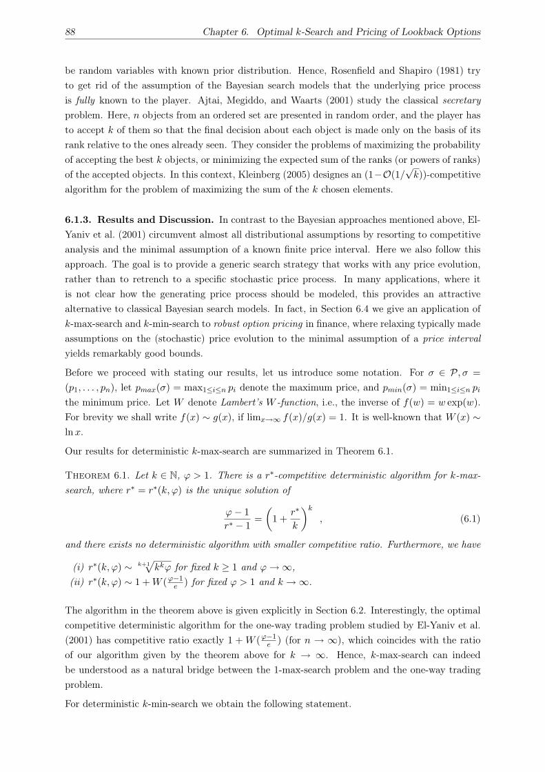
88 Chapter 6. Optimal k-Search and Pricing of Lookback Options
be random variables with known prior distribution. Hence, Rosenfield and Shapiro (1981) try
to get rid of the assumption of the Bayesian search models that the underlying price process
is fully known to the player. Ajtai, Megiddo, and Waarts (2001) study the classical secretary
problem. Here, n objects from an ordered set are presented in random order, and the player has
to accept k of them so that the final decision about each object is made only on the basis of its
rank relative to the ones already seen. They consider the problems of maximizing the probability
of accepting the best k objects, or minimizing the expected sum of the ranks (or powers of ranks)
of the accepted objects. In this context, Kleinberg (2005) designes an (1−O(1/√
k))-competitive
algorithm for the problem of maximizing the sum of the k chosen elements.
6.1.3. Results and Discussion. In contrast to the Bayesian approaches mentioned above, El-
Yaniv et al. (2001) circumvent almost all distributional assumptions by resorting to competitive
analysis and the minimal assumption of a known finite price interval. Here we also follow this
approach. The goal is to provide a generic search strategy that works with any price evolution,
rather than to retrench to a specific stochastic price process. In many applications, where it
is not clear how the generating price process should be modeled, this provides an attractive
alternative to classical Bayesian search models. In fact, in Section 6.4 we give an application of
k-max-search and k-min-search to robust option pricing in finance, where relaxing typically made
assumptions on the (stochastic) price evolution to the minimal assumption of a price interval
yields remarkably good bounds.
Before we proceed with stating our results, let us introduce some notation. For σ ∈ P, σ =
(p1, . . . , pn), let pmax(σ) = max1≤i≤n pi denote the maximum price, and pmin(σ) = min1≤i≤n pi
the minimum price. Let W denote Lambert’s W -function, i.e., the inverse of f(w) = w exp(w).
For brevity we shall write f(x) ∼ g(x), if limx→∞ f(x)/g(x) = 1. It is well-known that W (x) ∼lnx.
Our results for deterministic k-max-search are summarized in Theorem 6.1.
Theorem 6.1. Let k ∈ N, ϕ > 1. There is a r∗-competitive deterministic algorithm for k-max-
search, where r∗ = r∗(k, ϕ) is the unique solution of
ϕ− 1
r∗ − 1=
(1 +
r∗
k
)k
, (6.1)
and there exists no deterministic algorithm with smaller competitive ratio. Furthermore, we have
(i) r∗(k, ϕ) ∼ k+1√
kkϕ for fixed k ≥ 1 and ϕ→∞,
(ii) r∗(k, ϕ) ∼ 1 + W (ϕ−1e ) for fixed ϕ > 1 and k →∞.
The algorithm in the theorem above is given explicitly in Section 6.2. Interestingly, the optimal
competitive deterministic algorithm for the one-way trading problem studied by El-Yaniv et al.
(2001) has competitive ratio exactly 1 + W (ϕ−1e ) (for n → ∞), which coincides with the ratio
of our algorithm given by the theorem above for k → ∞. Hence, k-max-search can indeed
be understood as a natural bridge between the 1-max-search problem and the one-way trading
problem.
For deterministic k-min-search we obtain the following statement.
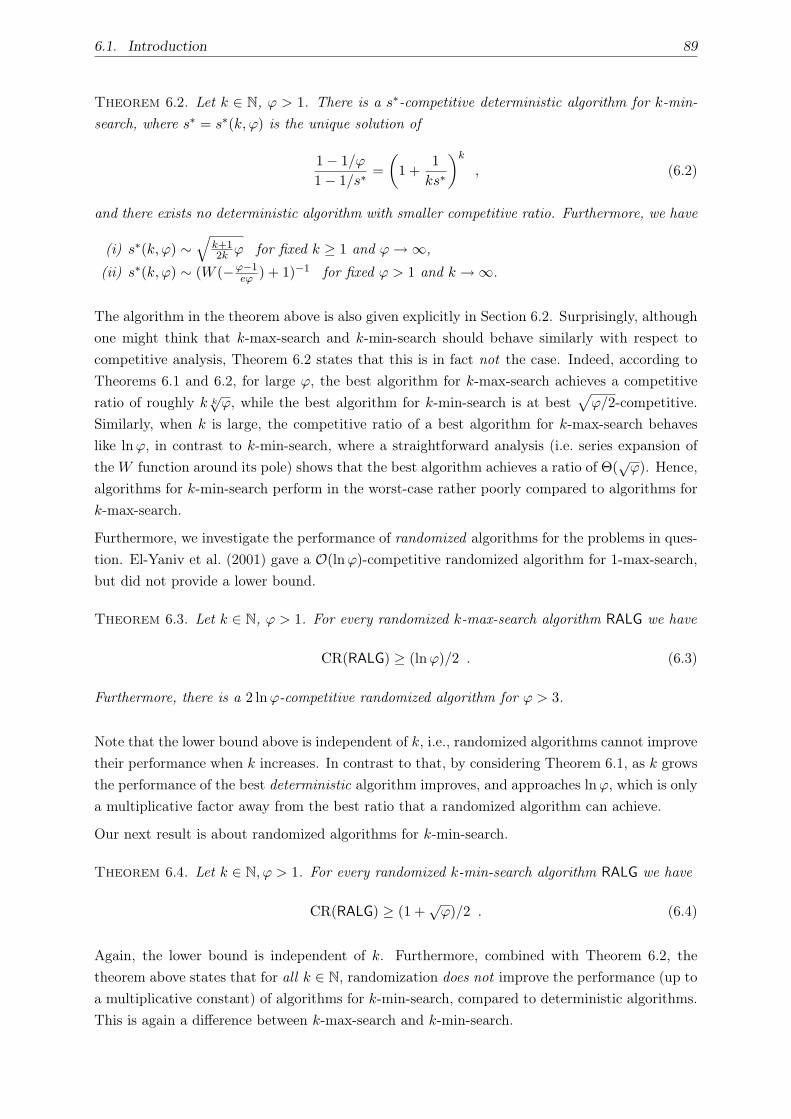
6.1. Introduction 89
Theorem 6.2. Let k ∈ N, ϕ > 1. There is a s∗-competitive deterministic algorithm for k-min-
search, where s∗ = s∗(k, ϕ) is the unique solution of
1− 1/ϕ
1− 1/s∗=
(1 +
1
ks∗
)k
, (6.2)
and there exists no deterministic algorithm with smaller competitive ratio. Furthermore, we have
(i) s∗(k, ϕ) ∼√
k+12k ϕ for fixed k ≥ 1 and ϕ→∞,
(ii) s∗(k, ϕ) ∼ (W (−ϕ−1eϕ ) + 1)−1 for fixed ϕ > 1 and k →∞.
The algorithm in the theorem above is also given explicitly in Section 6.2. Surprisingly, although
one might think that k-max-search and k-min-search should behave similarly with respect to
competitive analysis, Theorem 6.2 states that this is in fact not the case. Indeed, according to
Theorems 6.1 and 6.2, for large ϕ, the best algorithm for k-max-search achieves a competitive
ratio of roughly k k√
ϕ, while the best algorithm for k-min-search is at best√
ϕ/2-competitive.
Similarly, when k is large, the competitive ratio of a best algorithm for k-max-search behaves
like lnϕ, in contrast to k-min-search, where a straightforward analysis (i.e. series expansion of
the W function around its pole) shows that the best algorithm achieves a ratio of Θ(√
ϕ). Hence,
algorithms for k-min-search perform in the worst-case rather poorly compared to algorithms for
k-max-search.
Furthermore, we investigate the performance of randomized algorithms for the problems in ques-
tion. El-Yaniv et al. (2001) gave a O(lnϕ)-competitive randomized algorithm for 1-max-search,
but did not provide a lower bound.
Theorem 6.3. Let k ∈ N, ϕ > 1. For every randomized k-max-search algorithm RALG we have
CR(RALG) ≥ (lnϕ)/2 . (6.3)
Furthermore, there is a 2 lnϕ-competitive randomized algorithm for ϕ > 3.
Note that the lower bound above is independent of k, i.e., randomized algorithms cannot improve
their performance when k increases. In contrast to that, by considering Theorem 6.1, as k grows
the performance of the best deterministic algorithm improves, and approaches lnϕ, which is only
a multiplicative factor away from the best ratio that a randomized algorithm can achieve.
Our next result is about randomized algorithms for k-min-search.
Theorem 6.4. Let k ∈ N, ϕ > 1. For every randomized k-min-search algorithm RALG we have
CR(RALG) ≥ (1 +√
ϕ)/2 . (6.4)
Again, the lower bound is independent of k. Furthermore, combined with Theorem 6.2, the
theorem above states that for all k ∈ N, randomization does not improve the performance (up to
a multiplicative constant) of algorithms for k-min-search, compared to deterministic algorithms.
This is again a difference between k-max-search and k-min-search.
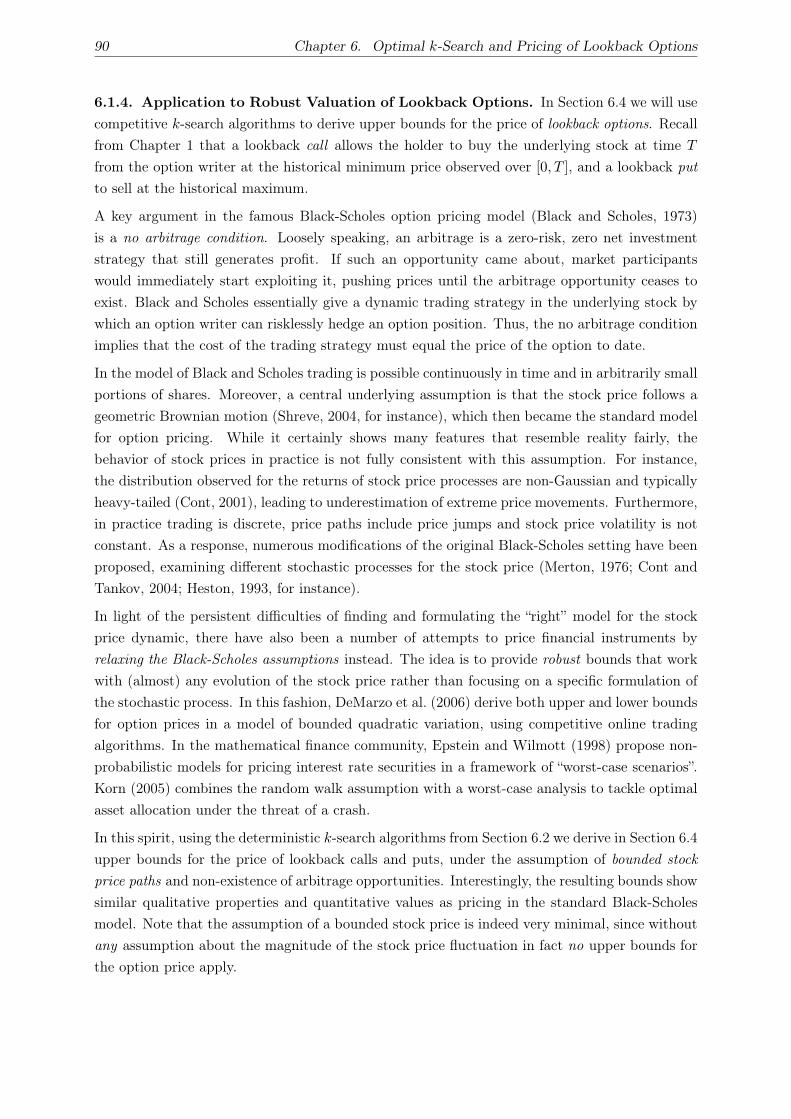
90 Chapter 6. Optimal k-Search and Pricing of Lookback Options
6.1.4. Application to Robust Valuation of Lookback Options. In Section 6.4 we will use
competitive k-search algorithms to derive upper bounds for the price of lookback options. Recall
from Chapter 1 that a lookback call allows the holder to buy the underlying stock at time T
from the option writer at the historical minimum price observed over [0, T ], and a lookback put
to sell at the historical maximum.
A key argument in the famous Black-Scholes option pricing model (Black and Scholes, 1973)
is a no arbitrage condition. Loosely speaking, an arbitrage is a zero-risk, zero net investment
strategy that still generates profit. If such an opportunity came about, market participants
would immediately start exploiting it, pushing prices until the arbitrage opportunity ceases to
exist. Black and Scholes essentially give a dynamic trading strategy in the underlying stock by
which an option writer can risklessly hedge an option position. Thus, the no arbitrage condition
implies that the cost of the trading strategy must equal the price of the option to date.
In the model of Black and Scholes trading is possible continuously in time and in arbitrarily small
portions of shares. Moreover, a central underlying assumption is that the stock price follows a
geometric Brownian motion (Shreve, 2004, for instance), which then became the standard model
for option pricing. While it certainly shows many features that resemble reality fairly, the
behavior of stock prices in practice is not fully consistent with this assumption. For instance,
the distribution observed for the returns of stock price processes are non-Gaussian and typically
heavy-tailed (Cont, 2001), leading to underestimation of extreme price movements. Furthermore,
in practice trading is discrete, price paths include price jumps and stock price volatility is not
constant. As a response, numerous modifications of the original Black-Scholes setting have been
proposed, examining different stochastic processes for the stock price (Merton, 1976; Cont and
Tankov, 2004; Heston, 1993, for instance).
In light of the persistent difficulties of finding and formulating the “right” model for the stock
price dynamic, there have also been a number of attempts to price financial instruments by
relaxing the Black-Scholes assumptions instead. The idea is to provide robust bounds that work
with (almost) any evolution of the stock price rather than focusing on a specific formulation of
the stochastic process. In this fashion, DeMarzo et al. (2006) derive both upper and lower bounds
for option prices in a model of bounded quadratic variation, using competitive online trading
algorithms. In the mathematical finance community, Epstein and Wilmott (1998) propose non-
probabilistic models for pricing interest rate securities in a framework of “worst-case scenarios”.
Korn (2005) combines the random walk assumption with a worst-case analysis to tackle optimal
asset allocation under the threat of a crash.
In this spirit, using the deterministic k-search algorithms from Section 6.2 we derive in Section 6.4
upper bounds for the price of lookback calls and puts, under the assumption of bounded stock
price paths and non-existence of arbitrage opportunities. Interestingly, the resulting bounds show
similar qualitative properties and quantitative values as pricing in the standard Black-Scholes
model. Note that the assumption of a bounded stock price is indeed very minimal, since without
any assumption about the magnitude of the stock price fluctuation in fact no upper bounds for
the option price apply.
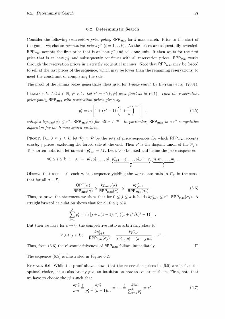
6.2. Deterministic Search 91
6.2. Deterministic Search
Consider the following reservation price policy RPPmax for k-max-search. Prior to the start of
the game, we choose reservation prices p∗i (i = 1 . . . k). As the prices are sequentially revealed,
RPPmax accepts the first price that is at least p∗1 and sells one unit. It then waits for the first
price that is at least p∗2, and subsequently continues with all reservation prices. RPPmax works
through the reservation prices in a strictly sequential manner. Note that RPPmax may be forced
to sell at the last prices of the sequence, which may be lower than the remaining reservations, to
meet the constraint of completing the sale.
The proof of the lemma below generalizes ideas used for 1-max-search by El-Yaniv et al. (2001).
Lemma 6.5. Let k ∈ N, ϕ > 1. Let r∗ = r∗(k, ϕ) be defined as in (6.1). Then the reservation
price policy RPPmax with reservation prices given by
p∗i = m
[1 + (r∗ − 1)
(1 +
r∗
k
)i−1]
, (6.5)
satisfies k pmax(σ) ≤ r∗ · RPPmax(σ) for all σ ∈ P. In particular, RPPmax is a r∗-competitive
algorithm for the k-max-search problem.
Proof. For 0 ≤ j ≤ k, let Pj ⊆ P be the sets of price sequences for which RPPmax accepts
exactly j prices, excluding the forced sale at the end. Then P is the disjoint union of the Pj ’s.
To shorten notation, let us write p∗k+1 = M . Let ε > 0 be fixed and define the price sequences
∀0 ≤ i ≤ k : σi = p∗1, p∗2, . . . , p
∗i , p∗i+1 − ε, . . . , p∗i+1 − ε︸ ︷︷ ︸
k
, m, m, . . . , m︸ ︷︷ ︸k
.
Observe that as ε → 0, each σj is a sequence yielding the worst-case ratio in Pj , in the sense
that for all σ ∈ Pj
OPT(σ)
RPPmax(σ)≤ kpmax(σ)
RPPmax(σ)≤
kp∗j+1
RPPmax(σj). (6.6)
Thus, to prove the statement we show that for 0 ≤ j ≤ k it holds kp∗j+1 ≤ r∗ · RPPmax(σj). A
straightforward calculation shows that for all 0 ≤ j ≤ k
j∑
i=1
p∗i = m[j + k(1− 1/r∗)
((1 + r∗/k)j − 1
)].
But then we have for ε→ 0, the competitive ratio is arbitrarily close to
∀ 0 ≤ j ≤ k :kp∗j+1
RPPmax(σj)=
kp∗j+1∑ji=1 p∗i + (k − j)m
= r∗ .
Thus, from (6.6) the r∗-competitiveness of RPPmax follows immediately.
The sequence (6.5) is illustrated in Figure 6.2.
Remark 6.6. While the proof above shows that the reservation prices in (6.5) are in fact the
optimal choice, let us also briefly give an intuition on how to construct them. First, note that
we have to choose the p∗i ’s such that
kp∗1km
!=
kp∗2p∗1 + (k − 1)m
!= · · · !
=kM
∑ki=1 p∗i
!= r∗. (6.7)
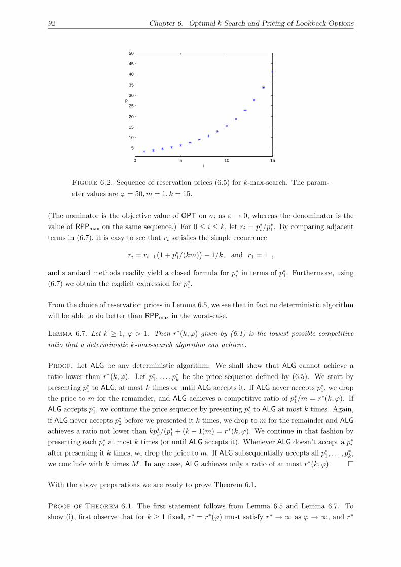
92 Chapter 6. Optimal k-Search and Pricing of Lookback Options
0 5 10 15
5
10
15
20
25
30
35
40
45
50
i
pi
Figure 6.2. Sequence of reservation prices (6.5) for k-max-search. The param-
eter values are ϕ = 50, m = 1, k = 15.
(The nominator is the objective value of OPT on σi as ε → 0, whereas the denominator is the
value of RPPmax on the same sequence.) For 0 ≤ i ≤ k, let ri = p∗i /p∗1. By comparing adjacent
terms in (6.7), it is easy to see that ri satisfies the simple recurrence
ri = ri−1
(1 + p∗1/(km)
)− 1/k, and r1 = 1 ,
and standard methods readily yield a closed formula for p∗i in terms of p∗1. Furthermore, using
(6.7) we obtain the explicit expression for p∗1.
From the choice of reservation prices in Lemma 6.5, we see that in fact no deterministic algorithm
will be able to do better than RPPmax in the worst-case.
Lemma 6.7. Let k ≥ 1, ϕ > 1. Then r∗(k, ϕ) given by (6.1) is the lowest possible competitive
ratio that a deterministic k-max-search algorithm can achieve.
Proof. Let ALG be any deterministic algorithm. We shall show that ALG cannot achieve a
ratio lower than r∗(k, ϕ). Let p∗1, . . . , p∗k be the price sequence defined by (6.5). We start by
presenting p∗1 to ALG, at most k times or until ALG accepts it. If ALG never accepts p∗1, we drop
the price to m for the remainder, and ALG achieves a competitive ratio of p∗1/m = r∗(k, ϕ). If
ALG accepts p∗1, we continue the price sequence by presenting p∗2 to ALG at most k times. Again,
if ALG never accepts p∗2 before we presented it k times, we drop to m for the remainder and ALG
achieves a ratio not lower than kp∗2/(p∗1 + (k − 1)m) = r∗(k, ϕ). We continue in that fashion by
presenting each p∗i at most k times (or until ALG accepts it). Whenever ALG doesn’t accept a p∗iafter presenting it k times, we drop the price to m. If ALG subsequentially accepts all p∗1, . . . , p
∗k,
we conclude with k times M . In any case, ALG achieves only a ratio of at most r∗(k, ϕ).
With the above preparations we are ready to prove Theorem 6.1.
Proof of Theorem 6.1. The first statement follows from Lemma 6.5 and Lemma 6.7. To
show (i), first observe that for k ≥ 1 fixed, r∗ = r∗(ϕ) must satisfy r∗ → ∞ as ϕ → ∞, and r∗

6.2. Deterministic Search 93
is an increasing function of ϕ. Let r+ = kk
k+1 k+1√
ϕ. Then, for ϕ→∞, we have
(r+ − 1)(1 +
r+
k
)k= (1 + o(1))
(k
kk+1 k+1
√ϕ ·(k− 1
k+1 k+1√
ϕ)k)
= (1 + o(1))ϕ .
Furthermore, let ε > 0 and set r− = (1 − ε)kk
k+1 k+1√
ϕ. A similar calculation as above shows
that for sufficiently large ϕ we have
(r− − 1)(1 +
r−k
)k≥ (1− 3kε) ϕ .
Thus, r = (1 + o(1)) kk
k+1 k+1√
ϕ indeed satisfies (6.1) for ϕ→∞. For the proof of (ii), note that
for k →∞ and ϕ fixed, equation (6.1) becomes (ϕ− 1)/(r∗ − 1) = er∗ , and thus
(ϕ− 1)/e = (r∗ − 1) er∗−1 .
The claim follows from the definition of the W -function.
Similarly, we can construct a reservation price policy RPPmin for k-min-search. Naturally, RPPmin
is modified such that it accepts the first price lower than the current reservation price.
Lemma 6.8. Let k ∈ N, ϕ > 1. Let s∗ = s∗(k, ϕ) be defined as in (6.2). Then the reservation
price policy RPPmin with reservation prices p∗1 > · · · > p∗k,
p∗i = M
[1−
(1− 1
s∗
)(1 +
1
ks∗
)i−1]
, (6.8)
satisfies RPPmin(σ) ≤ s∗(k, ϕ) · k pmin(σ), and is a s∗(k, ϕ)-competitive deterministic algorithm
for k-min-search.
Proof. The proof is analogous to the proof of Lemma 6.5. Again, for 0 ≤ j ≤ k, let Pj ⊆ Pbe the sets of price sequences for which RPPmin accepts exactly j prices, excluding the forced
sale at the end. To shorten notation, define p∗k+1 = m. Let ε > 0 be fixed and define the price
sequences
σi = p∗1, p∗2, . . . , p
∗i , p
∗i+1 + ε, . . . , p∗i+1 + ε︸ ︷︷ ︸
k
, M, . . . , M︸ ︷︷ ︸k
, for 0 ≤ i ≤ k .
As ε → 0, each σj is a sequence yielding the worst-case ratio in Pj , in the sense that for all
σ ∈ Pj , 0 ≤ j ≤ k,RPPmin(σ)
OPT(σ)≤ RPPmin(σ)
kpmin(σ)≤ RPPmin(σj)
kp∗j+1
. (6.9)
Straightforward calculation shows that for ε→ 0
∀ 0 ≤ j ≤ k :RPPmin(σj)
kp∗j+1
=
∑ji=1 p∗i + (k − j)M
kp∗j+1
= s∗ ,
and hence
∀σ ∈ P :RPPmin(σ)
kpmin(σ)≤ s∗ .
Since OPT(σ) ≥ kpmin(σ) for all σ ∈ P, this also implies that RPPmin is s∗-competitive.
The sequence (6.8) is illustrated in Figure 6.3.
Again, no deterministic algorithm can do better than RPPmin in Lemma 6.8.

94 Chapter 6. Optimal k-Search and Pricing of Lookback Options
0 5 10 15
5
10
15
20
25
30
35
40
45
50
i
pi
Figure 6.3. Sequence of reservation prices (6.8) for k-min-search. The parame-
ter values are ϕ = 50, m = 1, k = 15.
Lemma 6.9. Let k ≥ 1, ϕ > 1. Then s∗(k, ϕ) given by (6.2) is the lowest possible competitive
ratio that a deterministic k-min-search algorithm can achieve.
The proof of Lemma 6.9 is identical to the proof of Lemma 6.7, except that the adversary now
uses the prices defined by (6.8) and the roles of m and M are interchanged.
Using Lemma 6.8 and Lemma 6.9 we can now prove Theorem 6.2.
Proof of Theorem 6.2. The first part of the Theorem follows directly from Lemma 6.8 and
Lemma 6.9. To show (i), first observe that for k ≥ 1 fixed, s∗ = s∗(ϕ) must satisfy s∗ → ∞as ϕ → ∞, and s∗ is an increasing function of ϕ. With this assumption we can expand the
right-hand side of (6.2) with the binomial theorem to obtain
1− 1/ϕ
1− 1/s∗= 1 +
1
s∗+
k − 1
2k (s∗)2+ Θ
((s∗)−3
)=⇒ 1
ϕ=
k + 1
2k (s∗)2+ Θ
((s∗)−3
).
By solving this equation for s∗ we obtain (i). For the proof of (ii), first observe that for ϕ ≥ 1
fixed, s∗ = s∗(k) must satisfy s∗(k) ≤ C, for some constant C which may depend on ϕ. Indeed,
if s∗(k)→∞ with k →∞, then by taking limits on both sides of (6.2) yields
1− 1
ϕ= lim
k→∞
(1 +
1
ks∗(k)
)k
= 1 ,
which is a contradiction. Thus, s∗ = Θ(1) and we obtain from (6.2) by taking limits
1− 1/ϕ
1− 1/s∗= lim
k→∞
(1 +
1
ks∗
)k
= e1/s∗ ,
and (ii) follows immediately by the definition of the W -function.
6.3. Randomized Search
6.3.1. Lower Bound for Randomized k-max-search. We consider k = 1 first. The optimal
deterministic online algorithm achieves a competitive ratio of r∗(1, ϕ) =√
ϕ. As shown by El-
Yaniv et al. (2001), randomization can dramatically improve this. Assume for simplicity that

6.3. Randomized Search 95
ϕ = 2ℓ for some integer ℓ. For 0 ≤ j < ℓ let RPPmax(j) be the reservation price policy with
reservation m2j , and define EXPO to be a uniform probability mixture over RPPmax(j)ℓ−1j=0.
Lemma 6.10 (Levin, see El-Yaniv et al. (2001)). Algorithm EXPO is O(lnϕ)-competitive.
We shall prove that EXPO is in fact the optimal randomized online algorithm for 1-max-search.
We will use the following version of Yao’s principle (Yao, 1977).
Theorem 6.11 (Yao’s principle). For an online maximization problem denote by S the set of
possible input sequences, and by A the set of deterministic algorithms, and assume that S and Aare finite. Fix any probability distribution y(σ) on S, and let S be a random sequence according
to this distribution. Let RALG be any mixed strategy, given by a probability distribution on A.
Then,
CR(RALG) = maxσ∈S
OPT(σ)
E [RALG(σ)]≥(
maxALG∈A
E
[ALG(S)OPT(S)
])−1
. (6.10)
Note that the first expectation is taken with respect to the randomization of the algorithm RALG,
whereas the second expectation is taken with respect to the input distribution y(σ).
The reader is referred to standard textbooks for a proof (e.g. Chapter 6 and 8 of Borodin and El-
Yaniv (1998)). In words, Yao’s principle states that we obtain a lower bound on the competitive
ratio of the best randomized algorithm by calculating the performance of the best deterministic
algorithm for a chosen probability distribution of input sequences. Note that (6.10) gives a lower
bound for arbitrary chosen input distributions. However, only for well-chosen y’s we will obtain
strong lower bounds.
We first need to establish the following lemma on the representation of an arbitrary randomized
algorithm for k-search.
Lemma 6.12. Let RALG be a randomized algorithm for the k-max-search problem. Then RALG
can be represented by a probability distribution on the set of all deterministic algorithms for the
k-max-search problem.
Proof. The proof of the statement is along the lines of the proof of Theorem 1 in El-Yaniv
et al. (2001). Here we only sketch the proof idea. Using game-theoretic terminology, RALG
may be either a mixed strategy (a distribution on deterministic algorithms, from which one is
randomly chosen prior to the start of the game) or a behavioral strategy (where an independent
random choice may be made at each point during the game). As we have perfect recall in k-search
(player has no memory restrictions), k-search is a linear game. For linear games, every behavioral
strategy has an equivalent mixed algorithm. Thus, we can always assume that RALG is a mixed
strategy given by a probability distribution on the set of all deterministic algorithms.
The next lemma yields the desired lower bound.
Lemma 6.13. Let ϕ > 1. Every randomized 1-max-search algorithm RALG satisfies
CR(RALG) ≥ (lnϕ)/2 .

96 Chapter 6. Optimal k-Search and Pricing of Lookback Options
Proof. Let b > 1 and ℓ = logb ϕ. We define a finite approximation of I by Ib = mbi | i =
0 . . . ℓ, and let Pb =⋃
n≥k Inb . We consider the 1-max-search problem on Pb. As Pb is finite, also
the set of deterministic algorithms Ab is finite. For 0 ≤ i ≤ ℓ− 1, define sequences of length ℓ by
σi = mb0, . . . , mbi, m, . . . , m . (6.11)
Let Sb = σi | 0 ≤ i ≤ ℓ− 1 and define the probability distribution y on Pb by
y(σ) =
1/ℓ for σ ∈ Sb ,
0 otherwise .
Let ALG ∈ Ab. Note that for all 1 ≤ i ≤ ℓ, the first i prices of the sequences σj with j ≥ i − 1
coincide, and ALG cannot distinguish them up to time i. As ALG is deterministic, it follows that
if ALG accepts the i-th price in σℓ−1, it will accept the i-th price in all σj with j ≥ i− 1. Thus,
for every ALG, let 0 ≤ χ(ALG) ≤ ℓ − 1 be such that ALG accepts the (χ(ALG) + 1)-th price,
i.e. mbχ(ALG), in σℓ−1. ALG will then earn mbχ(ALG) on all σj with j ≥ χ(ALG), and m on all σj
with j < χ(ALG). To shorten notation, we write χ instead of χ(ALG) in the following. Thus, we
have
E
[ALG
OPT
]=
1
ℓ
χ−1∑
j=0
m
mbj+
ℓ−1∑
j=χ
mbχ
mbj
=
1
ℓ
[1− b−χ
1− b−1+
1− b−(ℓ−χ)
1− b−1
],
where the expectation E [·] is with respect to the probability distribution y(σ). If we consider the
above term as a function of χ, then it is easily verified that it attains its maximum at χ = ℓ/2.
Thus,
maxALG∈Ab
E
[ALG
OPT
]≤ 1
ℓ
(1− 1√
ϕ
)2b
b− 1≤ 1
lnϕ· 2b ln b
b− 1. (6.12)
Let Υb be the set of all randomized algorithms for 1-max-search with possible price sequences
Pb. By Lemma 6.12, each RALGb ∈ Υb may be given as a probability distribution on Ab. Since
Ab and Sb are both finite, we can apply Theorem 6.11. Thus, for all b > 1 and all RALGb ∈ Υb,
we have
CR(RALGb) ≥(
maxALG∈Ab
E
[ALG
OPT
])−1
≥ lnϕb− 1
2b ln b.
Let Υ be the set of all randomized algorithms for 1-max-search on P. Since for b→ 1, we have
Ab → A, Υb → Υ and (b− 1)/(2b ln b)→ 12 , the proof is completed.
In fact, Lemma 6.13 can be generalized to arbitrary k ≥ 1.
Lemma 6.14. Let k ∈ N, b > 1 and ϕ > 1. Let RALG be any randomized algorithm for
k-max-search. Then, we have
CR(RALG) ≥ (lnϕ)/2 .
Proof. Let 1 < b < ϕ and ℓ = logb ϕ. We define Pb and Ab as in the proof of Lemma 6.13. For
0 ≤ i ≤ ℓ− 1, define
σi = mb0, . . . , mb0
︸ ︷︷ ︸k
, . . . , mbi, . . . , mbi
︸ ︷︷ ︸k
, m, . . . , m︸ ︷︷ ︸k(ℓ−i−1)
. (6.13)

6.3. Randomized Search 97
Let Sb =⋃
0≤i≤ℓ−1 σi and define the probability distribution y on Pb by
y(σ) =
1/ℓ for σ ∈ Sb ,
0 otherwise .
Similarly as in the proof of Lemma 6.13, we characterize every algorithm ALG ∈ Ab by a vector
(χi)1≤i≤k where mbχi is the price for which ALG sells the i-th unit on σℓ−1. By construction,
we have χ1 ≤ · · · ≤ χk. (Recall that σℓ−1 is the sequence that is increasing until the very
end.) Note that for all 1 ≤ i ≤ ℓ, the sequences σj | j ≥ i − 1 are not distinguishable up
to time ik, since the first ik prices of those sequences are identical. Let 0 ≤ j ≤ ℓ − 1 and
t = maxi |χi ≤ j. When presented σj , ALG accepts all prices mbχi for which χi ≤ j. Hence,
we have OPT(σj) = kmbj and ALG(σj) = (k − t)m +∑t
s=1 mbχs , i.e. ALG can successfully sell
for its first t reservation prices. To abbreviate notation, let χ0 = 0 and χk+1 = ℓ, and define
δt = χt+1 − χt. Taking expectation with respect to y(σ), we have
E
[ALG
OPT
]=
1
ℓ
k∑
t=0
χt+1−1∑
j=χt
(k − t)m +∑t
s=1 mbχs
kmbj
=1
ℓ
k∑
t=0
(k − t +
∑ts=1 bχs
)∑δt−1j=0 b−j
kbχt
=1
ℓ
k∑
t=0
(k − t +
∑ts=1 bχs
)(1− b−δt)
kbχt(1− b−1).
Straightforward yet tedious algebra simplifies this expression to
E
[ALG
OPT
]=
∑kt=1 1− b−χt +
∑kt=1 1− b−(ℓ−χt)
ℓk(1− b−1),
and the maximum over χ1, . . . , χk is attained at χ1 = · · · = χk = ℓ/2. Thus, defining χ = ℓ/2
we have
maxALG∈Ab
E
[ALG
OPT
]≤ 1
ℓ
[1− b−χ
1− b−1+
1− b−(ℓ−χ)
1− b−1
]=
2b
ℓ (b− 1)
(1− 1√
ϕ
),
which is exactly (6.12) in the proof of Lemma 6.13. Thus, we can argue as in the remainder of
the proof of Lemma 6.13, and let again b → 1 to conclude that CR(RALG) ≥ (lnϕ)/2 for all
randomized algorithms RALG for k-max-search.
Giving an optimal randomized algorithm for k-max-search is straightforward. For 1 < b < ϕ
and ℓ = logb ϕ, EXPOk chooses j uniformly at random from 0, . . . , ℓ − 1, and sets all its k
reservation prices to mbj .
Lemma 6.15. Let k ∈ N. EXPOk is an asymptotically optimal randomized algorithm for the
k-max-search problem with CR(EXPOk) = lnϕ · (b−1)ln b
ϕϕ−1 .
Proof. We want to determine
CR(EXPOk) = maxσ∈P
R(σ), where R(σ) =OPT(σ)
E [EXPOk(σ)]. (6.14)

98 Chapter 6. Optimal k-Search and Pricing of Lookback Options
Obviously, a sequence σ that maximizes R is non-decreasing, since rearranging σ does not change
the objective value of OPT, but may increase the objective value of EXPOk. Let
σ = m, . . . , m︸ ︷︷ ︸k
, mb1, . . . , mb1
︸ ︷︷ ︸k
, mb2, . . . , mb2
︸ ︷︷ ︸k
, . . . , mbℓ−1, . . . , mbℓ−1
︸ ︷︷ ︸k
, M, . . . , M︸ ︷︷ ︸k
.
In the following, we will prove that σ is a worst-case sequence for (6.14). We will first show that
for every non-decreasing sequence σ = p1, p2, . . . , pN it holds
R(σ) ≤ R(σ σ) , (6.15)
where σ σ is the concatenation of σ and σ. Let P be the reservation price of EXPOk, and
let EXPOjk(σ) = E
[EXPOk(σ) | P = mbj
]. To see the first inequality we shall show that for all
0 ≤ j < ℓ,
EXPOjk(σ σ)
OPT(σ σ)≤ EXPO
jk(σ)
OPT(σ), (6.16)
which yields
1
R(σ)= E
[EXPOk(σ)
OPT(σ)
]≥ E
[EXPOk(σ σ)
OPT(σ σ)
]=
1
R(σ σ),
i.e., R(σ) ≤ R(σ σ). To see (6.16), note that if pl is the first price accepted by EXPOjk in σ, then
EXPOjk will also accept pl+1, . . . , pl+k−1. This follows from the property of σ being non-decreasing
and from the fact that all reservation prices of EXPOjk are identical. Now we distinguish two cases:
either l = N − k + 1 (i.e. EXPOjk accepts the last k prices in σ, possibly forced by the constraint
to finish the sale by the end of the sequence σ) or l < N −k +1 (i.e. EXPOjk can successfully sell
all k units for prices of at least its reservation price mbj). In the first case, EXPOjk(σ) = OPT(σ)
and (6.16) follows trivially, since we always have EXPOjk(σ σ) ≤ OPT(σ σ). In the second
case, OPT(σ σ) = kM ≥ OPT(σ) and EXPOjk(σ σ) = EXPO
jk(σ), since EXPO
jk accepted k
prices before the end of σ was reached, and it cannot accept any prices in the second part of
σ σ. Hence, (6.16) also holds in this case. This shows (6.15).
Now observe that for any non-decreasing σ we have
E [EXPOk(σ σ)] ≥ E [EXPOk(σ)] ,
since for every j algorithm EXPOjk accepts k prices in σ σ that are at least mbj , but in σ it
accepts k times exactly its reservation price mbj . Combined with the fact that OPT(σ σ) =
OPT(σ) = kM , this yields
R(σ σ) ≤ R(σ) .
With (6.15), this implies that σ is a worst-case sequence for (6.14). Therefore, we have
CR(EXPOk) = R(σ) =kM
1ℓ
∑ℓ−1j=0 kmbj
= ℓϕ (b− 1)
ϕ− 1= lnϕ
ϕ
ϕ− 1· (b− 1)
ln b,
since M = ϕm and bℓ = ϕ.
For ϕ > 3 and b < 3/2, we have ϕϕ−1
(b−1)ln b < 2, and hence combining Lemma 6.14 and 6.15 we
immediately obtain Theorem 6.3.

6.4. Robust Valuation of Lookback Options 99
6.3.2. Randomized k-Min-Search. The proof of the lower bound for k-min-search, Theo-
rem 6.4, uses an analogous version of Yao’s principle (see for instance Theorem 8.5 in Borodin
and El-Yaniv (1998)).
Theorem 6.16 (Yao’s principle for cost minimization problems). For an online cost minimization
problem Π, let the set of possible input sequences S and the set of deterministic algorithms
A be finite, and given by S = σ1, . . . , σn and A = ALG1, . . . ,ALGm. Fix any probability
distribution y(σ) on S. Let RALG be any mixed strategy, given by a probability distribution x(a)
on A. Then,
CR(RALG) = maxσ∈S
E [RALG(σ)]
OPT(σ)≥ min
ALG∈AE
[ALG
OPT
].
We are now ready to prove Theorem 6.4.
Proof of Theorem 6.4. We shall consider first the case k = 1. Let S = σ1, σ2 with
σ1 = m√
ϕ, M, . . . , M and σ2 = m√
ϕ, m, M, . . . , M ,
and let y(σ) be the uniform distribution on S. For i ∈ 1, 2, let ALGi be the reservation
price policy with reservation prices p∗1 = m√
ϕ and p∗2 = m, respectively. Obviously, the best
deterministic algorithm against the randomized input given by the distribution y(σ) behaves
either like ALG1 or ALG2. Since
E
[ALGi
OPT
]= (1 +
√ϕ)/2, i ∈ 1, 2 ,
the desired lower bound follows from the min-cost version of Yao’s principle. For general k ≥ 1,
we repeat the prices m√
ϕ and m in σ1 and σ2 k times each. Observe that in that case we can
partition the set of all deterministic algorithms into k + 1 equivalence classes, according to the
number price quotations accepted from the first k prices m√
ϕ, . . . , m√
ϕ, as σ1 and σ2 are not
distinguishable until the (k + 1)th price. Suppose ALG accepts j times the price m√
ϕ. Then we
have
E
[ALG
OPT
]=
1
2
(jm√
ϕ + (k − j)M
km√
ϕ+
jm√
ϕ + (k − j)m
km
)= (1 +
√ϕ)/2
for all 0 ≤ j ≤ k, and the lower bound follows again from Yao’s principle.
6.4. Robust Valuation of Lookback Options
In this section, we use the deterministic k-search algorithms from Section 6.2 to derive upper
bounds for the price of lookback options under the assumption of bounded stock price paths
and non-existence of arbitrage opportunities. We consider a discrete-time model of trading. For
simplicity we assume that the interest rate is zero. The price of the stock at time t ∈ 0, 1, . . . , Tis given by St, with S0 being the price when seller and buyer enter the option contract.
Recall that the holder of a lookback call has the right to buy shares from the option writer for
the price Smin = minSt | 0 ≤ t ≤ T. We shall assume that the lookback call is on k ≥ 1 units
of the underlying stock.
Note that since Smin ≤ ST , the option holder is never worse off executing the option at the
expiry date T (and then immediately selling the shares for ST ) rather than to forgo his option.
Hence, a lookback call option can always be considered as executed at expiry. This is in contrast

100 Chapter 6. Optimal k-Search and Pricing of Lookback Options
to a European call option, where the option holder is not interested in executing his option if
the price ST at expiry is below the pre-specified strike price K.
Neglecting stock price appreciation, upwards and downwards movement of the stock price is
equally likely. Consequently, we will assume a symmetric trading range [ϕ−1/2S0, ϕ1/2 S0] with
ϕ > 1. We shall refer to a stock price path that satisfies St ∈ [ϕ−1/2S0, ϕ1/2 S0] for all 1 ≤ t ≤ T
as a (S0, ϕ) price path.
Theorem 6.17. Assume (St)0≤t≤T is a (S0, ϕ) stock price path. Let s∗(k, ϕ) be given by (6.2),
and let
V ∗Call(S0, ϕ) = S0(s
∗(k, ϕ)− 1)/√
ϕ . (6.17)
Let V be the option premium paid at time t = 0 for a lookback call option on k shares expiring
at time T . Suppose we have V > V ∗Call(k, S0, ϕ). Then there exists an arbitrage opportunity for
the option writer, i.e., there is a zero-net-investment strategy which yields a profit for all (S0, ϕ)
stock price paths.
Proof. In the following, let Ct denote the money in the option writer’s cash account at time t.
At time t = 0, the option writer receives V from the option buyer, and we have C0 = V . The
option writer then successively buys k shares, one-by-one, applying RPPmin for k-min-search with
reservation prices as given by (6.8). Let H be the total sum of money spent for purchasing k units
of stock. By Lemma 6.8 we have H ≤ ks∗(k, ϕ)Smin. At time T the option holder purchases
k shares from the option writer for kSmin in cash. As noted above, a lookback call option can
always be considered executed at the expiration time T ; if the option holder does not execute
his option, the option writer simply sells the k shares again on the market for kST ≥ kSmin.
After everything has been settled, we have
CT = V −H + kSmin ≥ V + kSmin(1− s∗(k, ϕ)) .
Because of Smin ≥ S0/√
ϕ and V > V ∗Call(S0, ϕ), we conclude that CT > 0 for all possible (S0, ϕ)
stock price paths. Hence, this is indeed a zero net investment profit for the option writer on all
(S0, ϕ) stock price paths.
Under the no-arbitrage assumption, we immediately obtain an upper bound for the value of a
lookback call option.
Corollary 6.18. Under the no-arbitrage assumption, V ≤ V ∗Call(k, S0, ϕ), with V ∗
Call defined
in (6.17).
Using Lemma 6.5 and similar no-arbitrage arguments, also an upper bound for the price of a
lookback put option can be established.
Note that it is not possible to derive non-trivial lower bounds for lookback options in the bounded
stock price model, as a (S0, ϕ)-price path may stay at S0 throughout, making the option mature
worthless for the holder. To derive lower bounds, there must be a promised fluctuation of the
stock. In the classical Black-Scholes pricing model, this is given by the volatility of the Brownian
motion.

6.4. Robust Valuation of Lookback Options 101
We shall remark that in practice there is of course no trading range in which the stock price
stays with certainty; what we rather can give are trading ranges in which the price stays with
sufficiently high probability. V ∗Call is then to be understood as a bound for the option price up to
a certain residual risk. Note that whereas the Black-Scholes-type price (6.18), which shall be in
the next paragraph, has no such residual risk within the Black-Scholes model, it does certainly
have significant model risk due to the fact that the Black-Scholes assumptions might turn out to
be incorrect in the first place.
Comparison to Pricing in Black-Scholes Model. In the classical Black-Scholes setting,
Goldman, Sosin, and Gatto (1979) give closed form solutions for the value of lookback puts
and calls. Let σ be the volatility of the stock price, modeled by a geometric Brownian motion,
S(t) = S0 exp(−σ2t/2 + σB(t)), where B(t) is a standard Brownian motion. Let Φ(x) denote
the cumulative distribution function of the standard normal distribution. Then, for zero interest
rate, at time t = 0 the value of a lookback call on one share of stock, expiring at time T , is given
by
V BSCall(S0, T, σ) = S0
(2 Φ(σ
√T/2)− 1
). (6.18)
The hedging strategy is a certain roll-over replication strategy of a series of European call options.
Everytime the stock price hits a new all-time low, the hedger has to “roll-over” his position in
the call to one with a new strike. Interestingly, this kind of behavior to act only when a new
all-time low is reached resembles the behavior of RPPmin for k-min-search.
For a numerical comparison of the bound V ∗Call(k, S0, ϕ, T ) with the Black-Scholes-type pricing
formula (6.18), we choose the fluctuation rate ϕ = ϕ(T ) such that the expected trading range[E(min0≤t≤T St), E(max0≤t≤T St)
]of a geometric Brownian motion starting at S0 with volatility
σ is the interval[ϕ−1/2S0, ϕ
1/2S0
].
Figure 6.4 shows the results for σ = 0.2, S0 = 20 and k = 10. As can be seen from the graph, the
bound V ∗Call is qualitatively and quantitatively similar to the Black-Scholes-type pricing (6.18).
However, it is important to note that the two pricing formulas rely on two very different models.
In the Black-Scholes model, (6.18) is the correct price for a lookback option. On the other
hand, the key advantage of the price bound (6.17) are its weak modeling assumptions on the
price dynamics, and hence the price bound holds even in situations where the Black-Scholes
assumptions might break down. Certainly, both concepts have strengths and weaknesses, and a
good analysis consults both.
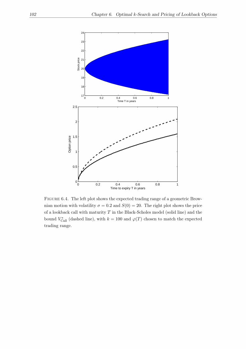
102 Chapter 6. Optimal k-Search and Pricing of Lookback Options
0 0.2 0.4 0.6 0.8 117
18
19
20
21
22
23
24
Time T in years
Sto
ck p
rice
0 0.2 0.4 0.6 0.8 10
0.5
1
1.5
2
2.5
Time to expiry T in years
Opt
ion
pric
e
Figure 6.4. The left plot shows the expected trading range of a geometric Brow-
nian motion with volatility σ = 0.2 and S(0) = 20. The right plot shows the price
of a lookback call with maturity T in the Black-Scholes model (solid line) and the
bound V ∗Call (dashed line), with k = 100 and ϕ(T ) chosen to match the expected
trading range.
APPENDIX A
Trading with Market Impact: Optimization of Expected Utility
In this section, we shall briefly outline expected utility optimization for the continuous-time
trading model with market impact introduced in Chapter 2, Section 2.2. Instead of the mean-
variance framework as in Chapters 2 and 3, a risk-reward balance is sought by optimizing the
expected utility of the final total amount captured. Different types of utility functions u(·) can
be used, and varying levels of risk aversion can be captured by parameters in u(·).As discussed in Chapters 1–3, mean-variance optimization retains practical advantages compared
to the optimization of expected utility. Mean and variance are very easily understood, and
correspond to how trade results are reported in practice. The broker/dealer can provide a
family of efficient strategies without assumptions on the clients’ utility and his other investment
activities. Furthermore, another problem with utility functions is that the risk-aversion depends
on the initial wealth, and in an institutional context it is very difficult to assign a value to this
wealth: is it the size of the individual order, the size of the day’s orders, or the client’s total
wealth under management?
For expected utility optimization, it is convenient to formulate the problem as a set of stochastic
differential equations, which incorporate a control function that we seek to optimize. As in
Chapter 2, suppose we are doing a sell program to complete at time T . Then the control, the
state variables, and the dynamic equations are
v(t) = rate of selling
x(t) = shares remaining to sell dx = −v dt
y(t) = dollars in bank account dy = (s− ηv) v dt
s(t) = stock price ds = σ dB
where dB is the increment of a Brownian motion, η is the coefficient of linear market impact,
and σ is absolute volatility. We begin at t = 0 with shares x(0) = X, cash y(0) = 0, and initial
stock price s(0) = S. The strategy v(t) must be adapted to the filtration of B.
We define the value function at time t in state (x, y, s) as the maximal achievable expected utility
of the final dollar amount in the bank account,
J(t, x, y, s) = maxv(t′)| t≤t′≤Ts.t. x(T )=0
E[u(y(T )
)∣∣t, x, y, s]
for a utility function u(·). The utility function is increasing (“more is always better than less”).
Its curvature reflects whether decision makers are risk averse (concave utility functions) or risk
seeking (convex utility functions).
103

104 Chapter A. Trading with Market Impact: Optimization of Expected Utility
Standard techniques (see e.g. textbooks by Yong and Zhou (1999); Fleming and Rishel (1975);
Korn (1997)) lead to the Hamilton-Jacobi Bellman (HJB) partial differential equation
0 = Jt +1
2σ2Jss + max
v
((sJy − Jx)v − ηJyv
2)
,
where subscripts denote partial derivatives. The quadratic is easily maximized explicitly, giving
the optimal trade rate
v∗ =sJy − Jx
2η Jy
and the final PDE for J(τ, x, y, s)
Jτ =1
2σ2Jss +
(sJy − Jx)2
4η Jy(A.1)
with τ = T − t. This is to be solved on τ > 0, with initial condition
J(0, x, y, s) = u(y) for x = 0 . (A.2)
It is crucial to handle the constraint x(T ) = 0 correctly. One way to do so is by adding the
expected cost of selling any remaining shares at time T with a linear liquidation strategy in an
extra time period [T, T + ǫ], and then let ǫ→ 0 (see Chapter 4, proof of Theorem 4.4).
While the PDE (A.1) is the same for all utility functions u(·), different solutions arise for different
choices of u(·) due to the initial condition (A.2). Schied and Schöneborn (2007) consider expo-
nential utility, u(y) = − exp(−αy) with risk-aversion parameter α > 0. This utility function has
constant absolute risk-aversion (CARA), and it can be shown that the static trading trajectories
of Almgren and Chriss (2000), see Lemma 2.2, are the optimal strategies; that is, the optimal
control v(t, x, y, s) = v(t, x) is deterministic and does not depend on the stock price s or the dol-
lar amount in the bank account y, which are driven by the realization of the Brownian motion.
For other utility functions with non-constant absolute risk-aversion (for instance, power utility
functions u(y) = (y1−γ − 1)/(1 − γ), 0 < γ 6= 1, or logarithmic utility u(y) = log y), optimal
strategies will in general be dynamic and may depend on s and y as well. As discussed by Li
and Ng (2000) and Zhou and Li (2000), the family of quadratic utility functions u(y) = ρy−λy2
may be used to derive mean-variance optimal strategies.
Problems in solving the problem for utility functions other than exponential utility arise from
the high nonlinearity of the PDE (A.1), especially the term Jy in the denominator; in the case of
exponential utility, Jy turns out to be constant (as a result of the constant risk-aversion), which
significantly simplifies the PDE. We leave the solution of the PDE for other utility functions and
the interpretation of these results as an open question for future research.

Notation
N, R natural and real numbers, respectively
log n, ln n logarithms of n to base 2 and e, respectively
o(f(n)) ,O(f(n)) Landau symbols
dom f domain of the function f
fx partial derivative ∂f
∂xof function f with respect to x
N (µ, σ2) normal distribution with mean µ and variance σ2
Φ cumulative distribution function of N (0, 1)
B(t) Brownian motion
P [E ] probability of event E
P [E | E ′] probability of event E conditioned on E ′
E [X] expectation of random variable X
E [X | E ] expectation of the random variable X conditioned on E
Var [X] variance of X, Var [X] = Eˆ
X2˜
− E [X]2
Var [X | E ] variance of the random variable X conditioned on E
Cov [X, Y ] covariance of the random variables X and Y ,
i.e. Cov [X, Y ] = E [XY ] − E [X] E [Y ]
ρ(X, Y ) correlation coefficient of the random variables X and Y ,
i.e. ρ(X, Y ) = Cov [X, Y ] /p
Var [X] Var [Y ]
Skew [X] skewness of the random variable X,
i.e. Skew [X] = Eˆ
(X − E [X])3˜
/p
Var [X]3
W (x) Lambert’s W-function 88
CR(ALG) competitive ratio of algorithm ALG 86
OPT offline optimum algorithm 86
105


List of Figures
2.1 Illustration of temporary market impact. . . . . . . . . . . . . . . . . . . . . . . . . . 14
2.2 Efficient frontiers for different values of market power µ, using single-update strategies. 22
2.3 Example of a single-update trading trajectory. . . . . . . . . . . . . . . . . . . . . . . 23
3.1 Illustration of temporary market impact in the discrete trading model. . . . . . . . . . 28
3.2 Illustration of the backwards optimization in Section 3.5. . . . . . . . . . . . . . . . . 43
3.3 Illustration of optimal adaptive trading for N = 4 time steps. . . . . . . . . . . . . . . 49
3.4 Adaptive efficient trading frontiers for different values of the market power. . . . . . . 50
3.5 Distributions of total cost corresponding to four points on the efficient trading frontier. 51
3.6 Sample path optimal adaptive strategy. . . . . . . . . . . . . . . . . . . . . . . . . . . 53
3.7 Comparison of J ′N (x, c) and JN (x, c). . . . . . . . . . . . . . . . . . . . . . . . . . . . 54
3.8 Comparison of J2(x, c) and J ′2(x, c) for different values of µ . . . . . . . . . . . . . . . 54
3.9 Comparison of single-update and multi-update adaptive frontiers . . . . . . . . . . . . 55
4.1 Sign-constrained static trading trajectories with drift estimate α . . . . . . . . . . . . 67
4.2 Sample trajectories of the Bayesian adaptive trading strategy with high drift. . . . . . 70
4.3 Sample trajectories of the Bayesian adaptive trading strategy with medium drift. . . . 70
6.1 Example of a bounded price path with m = 100, ϕ = 2. . . . . . . . . . . . . . . . . . 85
6.2 Sequence of reservation prices for k-max-search. . . . . . . . . . . . . . . . . . . . . . . 92
6.3 Sequence of reservation prices for k-min-search. . . . . . . . . . . . . . . . . . . . . . . 94
6.4 Expected trading range of a geometric Brownian motion with σ = 0.2 and S(0) = 20. 102
107


Bibliography
Ajtai, M., N. Megiddo, and O. Waarts (2001). Improved algorithms and analysis for secretary
problems and generalizations. SIAM Journal on Disc. Math. 14 (1), 1–27.
Almgren, R. and N. Chriss (1999). Value under liquidation. Risk 12 (12), 61–63.
Almgren, R. and N. Chriss (2000). Optimal execution of portfolio transactions. J. Risk 3 (2),
5–39.
Almgren, R. and N. Chriss (2003, June). Bidding principles. Risk .
Almgren, R. and J. Lorenz (2006). Bayesian adaptive trading with a daily cycle. J. Trading 1 (4),
38–46.
Almgren, R. and J. Lorenz (2007). Adaptive arrival price. Algorithmic Trading III , 59–66.
Almgren, R., C. Thum, E. Hauptmann, and H. Li (2005). Equity market impact. Risk 18 (7,
July), 57–62.
Almgren, R. F. (2003). Optimal execution with nonlinear impact functions and trading-enhanced
risk. Appl. Math. Fin. 10, 1–18.
Artzner, P., F. Delbaen, J.-M. Eber, and D. Heath (1999). Coherent measures of risk. Math.
Finance 9 (3), 203–228.
Artzner, P., F. Delbaen, J.-M. Eber, D. Heath, and H. Ku (2007). Coherent multiperiod risk
adjusted values and bellman’s principle. Annals of Operations Research 152 (1), 5–22.
Bajeux-Besnainou, I. and R. Portait (2002). Dynamic, deterministic and static optimal portfolio
strategies in a mean-variance framework under stochastic interest rates. In P. Willmott (Ed.),
New Directions in Mathematical Finance, pp. 101–114. New York: Wiley.
Bellman, R. (1957). Dynamic programming. Princeton Univeristy Press, Princeton, N. J.
Bertsimas, D., G. J. Lauprete, and A. Samarov (2004). Shortfall as a risk measure: properties,
optimization and applications. Journal of Economic Dynamics and Control 28 (7), 1353–1381.
Bertsimas, D. and A. W. Lo (1998). Optimal control of execution costs. J. Financial Markets 1,
1–50.
Bielecki, T. R., H. Jin, S. R. Pliska, and X. Y. Zhou (2005). Continuous-time mean-variance
portfolio selection with bankruptcy prohibition. Math. Finance 15 (2), 213–244.
Black, F. and M. S. Scholes (1973). The pricing of options and corporate liabilities. Journal of
Political Economy 81 (3), 637–54.
Borodin, A. and R. El-Yaniv (1998). Online computation and competitive analysis. New York:
Cambridge University Press.
109

110 Bibliography
Boyd, S. and L. Vandenberghe (2004). Convex optimization. Cambridge: Cambridge University
Press.
Butenko, S., A. Golodnikov, and S. Uryasev (2005). Optimal security liquidation algorithms.
Computational Optimization and Applications 32 (1), 9–27.
Cont, R. (2001). Empirical properties of asset returns: stylized facts and statistical issues.
Quantitative Finance 1, 223–236.
Cont, R. and P. Tankov (2004). Financial Modelling with Jump Processes. CRC Press.
Dantzig, G. B. and G. Infanger (1993). Multi-stage stochastic linear programs for portfolio
optimization. Ann. Oper. Res. 45 (1-4), 59–76.
DeMarzo, P., I. Kremer, and Y. Mansour (2006). Online trading algorithms and robust option
pricing. In Proc. of the ACM Symp. on Theory of Comp., STOC, pp. 477–486.
Densing, M. (2007). Hydro-Electric Power Plant Dispatch-Planning – Multi-Stage Stochastic
Programming with Time-Consistent Constraints on Risk. Ph. D. thesis, ETH Zurich. DISS.
ETH Nr. 17244.
Duffie, D. and H. R. Richardson (1991). Mean-variance hedging in continuous time. The Annals
of Applied Probability 1 (1), 1–15.
El-Yaniv, R., A. Fiat, R. M. Karp, and G. Turpin (2001). Optimal search and one-way trading
online algorithms. Algorithmica 30 (1), 101–139.
Engle, R. and R. Ferstenberg (2007). Execution risk. Journal of Portfolio Management (Winter).
Epstein, D. and P. Wilmott (1998). A new model for interest rates. International Journal of
Theoretical and Applied Finance 1 (2), 195–226.
Fleming, W. H. and R. W. Rishel (1975). Deterministic and Stochastic Optimal Control. Springer-
Verlag.
Fujiwara, H. and Y. Sekiguchi (2007). Average-Case Threat-Based Strategies for One-Way-
Trading.
Gandhi, D. K. and A. Saunders (1981). The superiority of stochastic dominance over mean vari-
ance efficiency criteria: Some clarifications. Journal of Business Finance and Accounting 8 (1),
p51 – 59.
Goldman, M. B., H. B. Sosin, and M. A. Gatto (1979). Path dependent options: "buy at the
low, sell at the high". The Journal of Finance 34 (5), 1111–1127.
He, H. and H. Mamaysky (2005). Dynamic trading policies with price impact. Journal of
Economic Dynamics and Control 29 (5), 891–930.
Heston, S. L. (1993). A closed-form solution for options with stochastic volatility with applica-
tions to bond and currency options. Rev. of Fin. Stud. 6 (2), 327–343.
Huberman, G. and W. Stanzl (2005). Optimal liquidity trading. Review of Finance 9 (2), 165–
200.
Hull, J. C. (2002). Options, Futures, and Other Derivatives. Prentice Hall.
Jin, H. and X. Zhou (2007). Stochastic Analysis and Applications, Chapter Continuous-Time
Markowitz’s Problems in an Incomplete Market, with No-Shorting Portfolios, pp. 435–459.

Bibliography 111
Springer-Verlag.
Karlin, A. R., M. S. Manasse, L. Rudolph, and D. D. Sleator (1988). Competitive snoopy caching.
Algorithmica 3 (1), 79–119.
Kissell, R. and M. Glantz (2003). Optimal Trading Strategies. Amacom.
Kissell, R. and R. Malamut (2005). Understanding the profit and loss distribution of trading
algorithms. In B. R. Bruce (Ed.), Algorithmic Trading, pp. 41–49. Institutional Investor.
Kleinberg, R. D. (2005). A multiple-choice secretary algorithm with applications to online auc-
tions. In SODA, pp. 630–631. SIAM.
Konishi, H. and N. Makimoto (2001). Optimal slice of a block trade. Journal of Risk 3 (4),
33–51.
Korn, R. (1997). Optimal Portfolios: Stochastic Models for Optimal Investment and Risk Man-
agement in Continuous Time. World Scientific.
Korn, R. (2005). Worst-case scenario investment for insurers. Insurance Math. Econom. 36 (1),
1–11.
Krokhmal, P. and S. Uryasev (2007). A sample-path approach to optimal position liquidation.
Annals of Operations Research 152 (1), 193–225.
Kroll, Y., H. Levy, and H. M. Markowitz (1984). Mean-variance versus direct utility maximiza-
tion. The Journal of Finance 39 (1), 47–61.
Leippold, M., F. Trojani, and P. Vanini (2004). A geometric approach to multiperiod mean
variance optimization of assets and liabilities. J. Econom. Dynam. Control 28 (6), 1079–1113.
Levy, H. (1992). Stochastic dominance and expected utility: Survey and analysis. Management
Science 38 (4), 555–593.
Levy, H. (2006). Stochastic dominance (Second ed.), Volume 12 of Studies in Risk and Uncer-
tainty. New York: Springer. Investment decision making under uncertainty.
Li, D. and W.-L. Ng (2000). Optimal dynamic portfolio selection: multiperiod mean-variance
formulation. Math. Finance 10 (3), 387–406.
Li, X. and X. Y. Zhou (2006). Continuous-time mean-variance efficiency: the 80% rule. Annals
of Applied Probability 16, 1751.
Li, X., X. Y. Zhou, and A. E. B. Lim (2002). Dynamic mean-variance portfolio selection with
no-shorting constraints. SIAM J. Control Optim. 40 (5), 1540–1555.
Lim, A. E. B. and X. Y. Zhou (2002). Mean-Variance Portfolio Selection with Random Param-
eters in a Complete Market. Mathematics of Operations Research 27 (1), 101–120.
Lintner, J. (1965). The valuation of risk assets and the selection of risky investments in stock
portfolios and capital budgets. The Review of Economics and Statistics 47 (1), 13–37.
Lippmann, S. A. and J. J. McCall (1976). The economics of job search: a survey. Economic
Inquiry XIV, 155–189.
Lippmann, S. A. and J. J. McCall (1981). The economics of uncertainty: selected topics and
probabilistic methods. Handbook of mathematical economics 1, 211–284.
112 Bibliography
Liptser, R. S. and A. N. Shiryaev (2001). Statistics of random processes. II (expanded ed.),
Volume 6 of Applications of Mathematics (New York). Berlin: Springer-Verlag. Applications,
Translated from the 1974 Russian original by A. B. Aries, Stochastic Modelling and Applied
Probability.
Lorenz, J., K. Panagiotou, and A. Steger (2007). Optimal algorithms for k-search with application
in option pricing. In Proc. of the 15th European Symp. on Algorithms (ESA 2007)., pp. 275–
286.
Lorenz, J., K. Panagiotou, and A. Steger (2008). Optimal algorithms for k-search with application
in option pricing. Algorithmica. To appear .
Maccheroni, F., M. Marinacci, A. Rustichini, and M. Taboga (2004). Portfolio selection with
monotone mean-variance preferences. ICER Working Papers - Applied Mathematics Series
27-2004, ICER - International Centre for Economic Research.
Madhavan, A. (2002). Vwap strategies. Transaction Performance: The Changing Face of Trading
Investment Guides Series. Institutional Investor Inc., 32–38.
Markowitz, H. (1952). Portfolio selection. The Journal of Finance 7 (1), 77–91.
Markowitz, H. M. (1959). Portfolio selection: Efficient diversification of investments. Cowles
Foundation for Research in Economics at Yale University, Monograph 16. New York: John
Wiley & Sons Inc.
Markowitz, H. M. (1991). Foundations of portfolio theory. Journal of Finance 46 (2), 469–77.
Merton, R. C. (1969). Lifetime portfolio selection under uncertainty: The continuous-time case.
The Review of Economics and Statistics 51 (3), 247–257.
Merton, R. C. (1971). Optimum consumption and portfolio rules in a continuous-time model.
Journal of Economic Theory 3 (4), 373–413.
Merton, R. C. (1972). An analytic derivation of the efficient portfolio frontier. The Journal of
Financial and Quantitative Analysis 7 (4), 1851–1872.
Merton, R. C. (1976). Option pricing when underlying stock returns are discontinuous. Journal
of Financial Economics 3 (1-2), 125–144.
Mossin, J. (1966). Equilibrium in a capital asset market. Econometrica 34 (4), 768–783.
Mossin, J. (1968). Optimal multiperiod portfolio policies. The Journal of Business 41 (2), 215–
229.
Oksendal, B. (2003). Stochastic differential equations (Sixth ed.). Universitext. Berlin: Springer-
Verlag. An introduction with applications.
Perold, A. F. (1988). The implementation shortfall: Paper versus reality. Journal of Portfolio
Management 14 (3), 4–9.
Pliska, S. R. (1986). A stochastic calculus model of continuous trading: optimal portfolios. Math.
Oper. Res. 11 (2), 370–382.
Richardson, H. R. (1989). A minimum variance result in continuous trading portfolio optimiza-
tion. Management Sci. 35 (9), 1045–1055.

Bibliography 113
Rosenfield, D. B. and R. D. Shapiro (1981). Optimal adaptive price search. Journal of Economic
Theory 25 (1), 1–20.
Samuelson, P. A. (1969). Lifetime portfolio selection by dynamic stochastic programming. The
Review of Economics and Statistics 51 (3), 239–246.
Schied, A. and T. Schöneborn (2007). Optimal portfolio liquidation for cara investors.
Schweizer, M. (1995). Variance-optimal hedging in discrete time. Math. Oper. Res. 20 (1), 1–32.
Sharpe, W. F. (1964). Capital asset prices: A theory of market equilibrium under conditions of
risk. The Journal of Finance 19 (3), 425–442.
Shreve, S. E. (2004). Stochastic calculus for finance. II. Springer Finance. New York: Springer-
Verlag. Continuous-time models.
Sleator, D. D. and R. E. Tarjan (1985). Amortized efficiency of list update and paging rules.
Comm. ACM 28 (2), 202–208.
Steinbach, M. C. (2001). Markowitz revisited: mean-variance models in financial portfolio anal-
ysis. SIAM Rev. 43 (1), 31–85.
The Economist (2005). The march of the robo-traders. In The Economist Technology Quarterly,
September 17th, pp. 13. The Economist.
The Economist (2007). Algorithmic trading: Ahead of the tape. In The Economist, June 21st,
pp. 85. The Economist.
von Neumann, J. and O. Morgenstern (1953). Theory of Games and Economic Behavior, 3rd ed.
Princeton: Princeton University Press.
Walia, N. (2006). Optimal trading: Dynamic stock liquidation strategies. Senior thesis, Princeton
University.
Wan, F. Y. M. (1995). Introduction to the calculus of variations and its applications. Chapman
and Hall Mathematics Series. New York: Chapman & Hall.
White, D. J. (1998). A parametric characterization of mean-variance efficient solutions for general
feasible action sets. Journal of Multi-Criteria Decision Analysis 7 (2), 109–119.
Yao, A. C. C. (1977). Probabilistic computations: toward a unified measure of complexity. In
18th Symp. on Foundations of Comp. Sci. (1977), pp. 222–227. IEEE Computer Society.
Yao, A. C. C. (1980). New algorithms for bin packing. J. Assoc. Comput. Mach. 27 (2), 207–227.
Yong, J. and X. Y. Zhou (1999). Stochastic controls: Hamiltonian systems and HJB equations.
Springer-Verlag.
Zhou, X. Y. and D. Li (2000). Continuous-time mean-variance portfolio selection: a stochastic
LQ framework. Appl. Math. Optim. 42 (1), 19–33.
Zhou, X. Y. and G. Yin (2003). Markowitz’s mean-variance portfolio selection with regime
switching: A continuous-time model. SIAM Journal on Control and Optimization 42 (4),
1466–1482.


Curriculum Vitae
Julian Michael Lorenz
born on December 19, 1978 in Pfaffenhofen a.d. Ilm, Germany
1987 – 1998 Secondary Education
Schyrengymnasium Pfaffenhofen, Germany
1998 – 1999 Mandatory Military / Civilian Service
BRK Pfaffenhofen
1999 – 2004 Studies in Mathematics at TU München, Germany
Degree: Diplom-Mathematiker
Scholarship of German National Academic Foundation
(Studienstiftung des Deutschen Volkes)
2003 Studies at National University of Singapore, Singapore
LAOTSE Exchange Program
since March 2005 Ph.D. student at ETH Zürich, Switzerland
115