Optimal Taxation with Risky Human Capital∗

Marek KapickaU.C. Santa Barbara

and CERGE-EI

Julian NeiraUniversity of Exeter

March 25, 2015

Abstract

We study optimal tax policies in a life-cycle economy with risky human capitaland permanent ability differences, where both ability and learning effort are privateinformation of the agents. The optimal policies balance several goals: redistributionacross agents, insurance against human capital shocks, incentives to accumulate hu-man capital, and incentives to work. We show that, in the optimum, i) high-abilityagents face risky consumption in order to elicit learning effort while low-abilityagents are insured, ii) high-ability agents face a higher savings tax to discouragethem from self-insuring, iii) under certain conditions, the inverse marginal labor in-come tax rate follows a random walk, and iv) the “no distortion at the top” resultdoes not apply if discouraging labor supply increases incentives to invest in humancapital. Quantitatively, we find large welfare gains for the U.S. from switching to anoptimal tax system.

J.E.L Codes: E6, H2Keywords: optimal taxation, income taxation, human capital

∗A previous version of this paper was circulated under the title Optimal Taxation in a Life-Cycle Economywith Endogenous Human Capital Formation. We are grateful to Laurence Ales, Javier Birchenall, AspenGorry, Finn Kydland, Ioana Marinescu, Gareth Myles, Peter Rupert, B. Ravikumar, Christian Siegel, RishSinghania, Ali Shourideh, Aleh Tsyvinski, Andres Zambrano and Yuzhe Zhang for insightful comments,as well as to seminar participants at the NBER Summer Institute, Stony Brook, the St. Louis Fed, theChicago Fed, U. of Los Andes, SED, Midwest Macro, LAEF and other seminars and conferences. Allerrors are our own.

1

1 Introduction

Models of life-cycle economies with agents who have permanent differences in ability

and face shocks to their human capital have been successful in understanding and quan-

tifying the sources of inequality over the life cycle. Huggett, Ventura, and Yaron (2011)

show that such a model is able to account for key empirical features of the dynamics

of earnings and consumption. We show that this model is also a useful and tractable

framework for studying optimal taxation. We assume that the government’s choices

are limited by two frictions: a standard Mirrleesean private information friction where

ability and labor effort are unobservable by the government, and a moral hazard fric-

tion where human capital investments (learning effort) and human capital shocks are also

unobservable by the government. In the optimum, the government faces a nontrivial

problem of balancing several competing objectives: redistribution of resources across

agents of different abilities; provision of insurance against human capital shocks; provi-

sion of incentives to accumulate human capital; and provision of incentives to elicit high

labor effort from agents with high human capital or ability.

We calibrate a two period version of the model to match a number of moments of

the U.S. economy (a ”status quo” model) and investigate the optimal tax policies and

efficient allocations. We find that it is optimal to provide high learning effort only for

about top 1% of agents. This is achieved mainly by making their consumption very

risky relative to the status quo economy. Specifically, high-ability agents face very low

consumption after very low realizations of human capital shocks, and this gives them

incentives to increase their learning effort. On the other hand, second period utility

is also low for very high realizations of human capital shocks, where the provision of

high labor effort becomes important. This conflicts with the government’s desire to elicit

high learning effort. For middle-ability agents, consumption risk is lower but still higher

than in the status quo economy. However, the incentives to provide high labor effort after

high human capital shocks lower their learning effort below the status quo economy. For

low-ability agents the desire to provide consumption insurance dominates, and they also

choose a relatively low learning effort. The private information friction interacts with the

moral hazard friction by limiting the amount of consumption risk that high-ability agents

face: in its absence, high ability agents would face even more consumption risk, and their

2

learning effort would be higher. Interestingly, our results regarding the distribution of

consumption risk stand in contrast to some of the previous literature with exogenous

i.i.d. productivity shocks (for example, Albanesi and Sleet (2006)) where high-ability

agents typically have more consumption insurance.

Following Werning (2011), we show that efficient allocation can be implemented by a

tax system with nonlinear income and capital taxes, where income taxes depend on the

realized human capital shock. Higher ability agents also face a higher marginal savings

tax rate to deter them from self insuring against their consumption risk. When the utility

function is additively separable in labor effort and learning effort, we show theoretically

that the inverse of the labor wedge follows a random walk, implying that the expected

labor wedge increases with age. This result is, to the best of our knowledge, novel

and allows us to identify a new role of age-dependent taxes: they correct the undesired

distortion in the intertemporal labor effort margin implied by a positive intertemporal

wedge. The intuition is as follows. A positive savings tax increases the present value

of future labor income, acting thus as a labor subsidy. Hence, the optimal future labor

wedge increases to “correct” for this. The second period marginal labor income tax rate

is decreasing in human capital shocks. The tax rate is decreasing faster for higher ability

agents, reflecting the fact that their consumption is more sensitive to human capital

shock realizations. We also show that the well-known “no distortion at the top” result

from the Mirrleesean literature does not apply if the utility function is not additively

separable in labor effort and learning effort. If, for example, discouraging labor effort

increases incentives to invest in human capital, even the “top” agent will optimally face

a positive marginal tax.

We find large welfare gains from implementing the efficient tax system. The unborn

agent is indifferent between the efficient tax system and the status quo economy with

4.5% higher consumption in every period and state of the world. We shut down each of the

two frictions and find that the private information friction is significantly more costly

than the moral hazard friction.

In solving the model we extend the method developed in Bohácek and Kapicka (2008)

(for riskless observable human capital) and Kapicka (2015) (for riskless unobservable

human capital). Both papers show that with a first-order approach one can partially

separate the redistributional dimension of the optimal tax problem, where the social

3

planner redistributes resources across agents, and the dynamic dimension of the optimal

tax problem, where the social planner chooses the optimal sequences of labor effort and

learning effort. The result relies on the assumption that abilities are permanent. The

assumption that human capital is observable is also important for preserving tractability.

It is, however, worth noting that due to unobservability of learning effort the model

shares some features typically associated with models with unobservable human capital,

namely that the incentives to accumulate human capital must be provided indirectly,

through income taxes. There is no scope for human capital subsidies in the model.

1.1 Relationship to the existing literature

We build on a large literature that looks at models with Ben-Porath’s (1967) technol-

ogy for human capital formation. Properly parameterized life-cycle versions of such

economies have been studied by Huggett, Ventura, and Yaron (2006) and Huggett, Ven-

tura, and Yaron (2011) who are able to quantitatively account for the hump-shaped pro-

file of average earnings and an increase in the earnings dispersion and skewness over the

life-cycle. Moreover, the stochastic process for earnings generated by the model is consis-

tent with both leading statistical models, the RIP (restricted income profile) models (see

e.g. MaCurdy (1982), Storesletten, Telmer, and Yaron (2004)) and the HIP (heterogeneous

income profile) models (see e.g. Lillard and Weiss (1979), Guvenen (2007)).1 Finally, the

Ben-Porath framework is also consistent with the increased dispersion in consumption

over the life-cycle, as documented by Aguiar and Hurst (2013) or Primiceri and van Rens

(2009). Our paper takes the economy with risky human capital and permanent ability

differences as a starting point for the optimal taxation analysis.

On the normative side, the paper uses the Mirrlees approach (Mirrlees (1971),Mir-

rlees (1976)) to optimal taxation. Recent literature has mostly focused on cases when

the individual skills are exogenous.2 In contrast, this paper focuses on a case when

individual skills are endogenous. Recent related contributions include Grochulski and

1The difference between RIP and HIP models is that in HIP models people face heterogeneous life-cycleearning profiles, while in RIP models individuals face similar life-cycle earning profiles.

2Main contributions include Golosov, Kocherlakota, and Tsyvinski (2003), Kocherlakota (2005), Al-banesi and Sleet (2006), Battaglini and Coate (2008), Farhi and Werning (2005), Werning (2007)). Golosov,Tsyvinski, and Troshkin (2015) and Farhi and Werning (2013) analyze optimal taxation in an environmentwhere individual skills are Markov.

4

Piskorski (2010) who study a problem with unobservable risky human capital. However,

investment in human capital in their model is only possible in the initial period and the

dynamics in the remaining periods are technically similar to the models with exogenous

skills. da Costa and Maestri (2007) consider a two-period economy with human capi-

tal investment where all risk is attributed to stochastic productive abilities. Stantcheva

(2015a) also studies optimal taxation with risky abilities and a Ben-Porath technology.

Human capital investments in her model are observable, and the model thus allows for

direct human capital subsidies. In our paper the source of risk are human capital shocks

while abilities are deterministic. Observable and risky human capital is also studied

by Findeisen and Sachs (2013), Findeisen and Sachs (2014) and Stantcheva (2015b), who

assume that human capital investments are in terms of goods, rather than time. Envi-

ronments with riskless human capital but a richer human capital technology have been

previously studied by Bohácek and Kapicka (2008) and Kapicka (2015).3 While each of

those models captures some important component of endogenous skill formation, nei-

ther of them is rich enough to fully capture the earnings and consumption dynamics

observed in the data. Our paper is also related to research on optimal Ramsey taxation

with endogenous human capital, such as Gorry and Oberfield (2012), Peterman (2012),

and Krueger and Ludwig (2013). This literature is able to consider richer frameworks

than ours by restricting taxes to specific functional forms. We view this line of research

as complementary to ours.

A related literature has studied the impact of moral hazard on optimal tax structures.

In Abraham, Koehne, and Pavoni (2012), hidden effort affects risky labor income out-

comes whereas in Albanesi (2007) hidden effort affects risky physical capital outcomes.

In contrast, our paper focuses on the interaction between moral hazard and private in-

formation. Another related study is Shourideh (2011), who studies an economy with

unobservable risky physical capital investments and unobservable abilities. Our paper

is technically related to his in that he also considers the interplay between moral haz-

ard and private information frictions. However, an important difference between hidden

savings and hidden human capital investments is that hidden savings imply hidden con-

3Kapicka (2006) analyzes the optimal steady state allocations in a similar environment with unobserv-able human capital and a restriction that the government can only use current income taxes and agentscannot borrow or save. See also Diamond and Mirrlees (2002) who analyze unobservable human capitalinvestments in a static framework.

5

sumption. Hidden consumption, in turn, implies that incentive compatibility constraints

might be upward binding, potentially changing the nature of the redistributive problem.

2 The Model

Consider the following life-cycle economy. Agents live for two periods. They like to

consume, dislike working and exerting learning effort, and have preferences given by

U(c1)−V(`1, e1) + βE [U(c2)−V(`2, 0)] , (1)

where j is age, cj is consumption, `j is labor effort, and ej is learning effort. The function

U is strictly increasing, strictly concave, and differentiable. The function V is strictly

increasing, strictly convex, and differentiable in both arguments. We further restrict the

function V by assuming that, conditionally on the learning effort being zero, the function

V exhibits a constant Frisch elasticity of labor γ(`, e) = V`(`,e)`V``(`,e) :

Assumption 1. The elasticity of labor effort γ(`, 0) is independent of `.

An agent’s earnings yj are determined by the agent’s ability a, current human capital

hj, and current labor effort `j:

yj = ahj`j. (2)

Ability is constant over an agent’s lifetime and is known to the agents at the beginning

of the first period. The ability has continuous support A = (a, a), with a possibly being

infinite. All agents are born with the same initial human capital h1. Human capital in

the second period h2 has continuous support H = (h, h), with h possibly infinite, and

depends on an idiosyncratic human capital depreciation shock z2, initial human capital

h1, and on learning effort e1:

h2 = exp(z2)F(h1, e1). (3)

The function F is strictly increasing, strictly concave, and differentiable in both argu-

ments. As is standard in the moral hazard literature, we transform the state-space repre-

sentation of the problem to work directly with the distribution induced over h2. To that

6

end, we construct a probability density function of human capital in the second period

conditional on first period effort and denote it p(h2|e1). The derivative of the density

with respect to effort pe(h|e) exists, and we assume that the conditional distribution of

the second period human capital satisfies the Monotone Likelihood Ratio Property:

Assumption 2 (MLRP). pe(h|e)p(h|e) is strictly increasing in h for all e.

The MLRP property has the usual interpretation that higher effort induces a more

favorable distribution of human capital outcomes.

This economy is identical to Huggett, Ventura, and Yaron (2011), with two exceptions.

First, this model includes leisure. That is essential for thinking about optimal taxation.

Second, the ability a affects earnings directly, rather than indirectly through the human

capital production function. That is irrelevant in the incomplete markets economy stud-

ied by Huggett, Ventura, and Yaron (2011) if the human capital production function

takes the Ben-Porath form.4 However, both formulations have different implications in

a Mirrleesean economy with private information and observable human capital where

it makes a difference whether h or ha is observed.5 The formulation chosen in this pa-

per has the advantage that it is entirely consistent with the existing Mirrleesean optimal

taxation literature.

Our preferred interpretation of observable risky human capital is the observability of

a person’s industry, firm, or occupation. Human capital shocks then take the interpre-

tation of shocks to industries, firms, or occupations. Support for this view comes from

the literature which argues that human capital is occupation, firm, or industry-specific

(see Jacobson, LaLonde, and Sullivan (1993), Neal (1995), Parent (2000), Poletaev and

Robinson (2008), and Kambourov and Manovskii (2009)).

4To see that both formulations are isomorphic, let F(h, e) = h + (eh)α. Redefine human capital asfollows: Let h = ha and a = a1−α. Then the law of motion for human capital is F(h, e) = h + a(eh)α, andthe earnings are y = h`, identical to the ones in Huggett, Ventura, and Yaron (2011).

5Both formulations are again isomorphic if both h and a are either observable or unobservable. Thefirst case is inconsistent with the Mirrleesean framework, while the second one would be extremely hardto solve in general.

7

3 Efficient Allocations

The information structure is as follows: ability a, labor effort `1 and `2, learning effort e1

and e2, and human capital shock z2 are private information of the agent. Consumption

c1 and c2, earnings y1 and y2, and human capital h1 and h2, are publicly observable.

Agents report their ability level to the social planner in the first period. An agent’s true

ability is denoted by a whereas a denotes the ability report.

An allocation (c, y) consists of consumption c = {c1(a), c2(a, h2)} and earnings y =

{y1(a), y2(a, h2)}. Consumption and earnings in the first period are conditional on ability

report a ∈ A. In the second period they are both conditional on the ability report in the

first period and realization of human capital in the second period, h2 ∈ H. Define the

lifetime utility of an a-type agent who reports ability a and exerts effort e as W(a, e|a),where

W(a, e|a) ≡ U(c1(a))−V(

y1(a)ah1

, e)+ β

∫H

[U (c2(a, h2))−V

(y2(a, h2)

ah2, 0)]

p(h2|e)dh2.

Effort in the second period is trivially equal to zero. The first period effort e1(a|a)maximizes the lifetime utility of an a−type agent who reports a:

e1(a|a) ≡ arg maxe

W(a, e|a). (4)

By the revelation principle, we restrict attention to the allocations that are incentive

compatible, i.e. where the agent prefers to tell the truth about his ability:

W(a, e1(a|a)|a) ≥W(a, e1(a|a)|a) ∀a, a ∈ A. (5)

In order to reduce notational complexity we define the utility maximizing effort plan

conditional on truthtelling by e1(a) ≡ e1(a|a), and let W(a) = W(a, e(a)|a) be the corre-

sponding truthteller’s lifetime utility.

An allocation is feasible if it satisfies the resource constraint

∫A

[c1(a)− y1(a) + R−1

∫H[c2(a, h2)− y2(a, h2)] p(h2|e1(a)) dh2

]q(a) da ≤ 0. (6)

8

where R is the gross interest rate. For simplicity, we assume that R = β−1.

The social welfare function is simply the expected utility of an agent who does not

yet know his ability:

W =∫

AW(a)q(a) da. (7)

Definition 1. An allocation is constrained efficient if it maximizes welfare (7) subject to the

resource constraint (6) and the incentive compatibility constraint (5), where the learning effort is

given by (4).

First-Order Approach. The first-order approach replaces the constraints (4) and (5)

with two conditions. The first one is the first-order condition in effort and says that,

at the optimum, the marginal costs of learning effort must be equal to the expected

marginal benefit of learning effort (given by the additional utility arising from the fact

that the distribution of future human capital shocks is now more favorable):

Ve

(y1(a)ah1

, e1(a))= β

∫H

[U(c2(a, h2))−V

(y2(a, h2)

ah2, 0)]

pe(h2|e1(a)) dh2. (8)

The second condition is an envelope condition governing how the lifetime utility needs

to vary with ability in order to deter the agent from misreporting his type. Let W(a)

denote the lifetime utility of the least able agent. The envelope condition is

W(a) = W(a)+∫ a

a

{V`

(y1(a)ah1

, e1(a))

y1(a)ah1

+ β∫

HV`

(y2(a, h2)

ah2, 0)

y2(a, h2)

ah2p(h2|e1(a)) dh2

}daa

. (9)

The envelope condition states that the variation in lifetime utility for an agent a is the

lifetime utility of the least able agent plus the informational rent the agent obtains from

having his given ability level. Replacing the incentive constraint with the first order

condition in effort and the envelope condition leads to a relaxed planning problem:

Definition 2. An allocation solves the relaxed planning problem if it maximizes welfare (7)

subject to the resource constraint (6), the first-order condition in effort (8) and the envelope

9

condition (9) .

For now, we assume that the first-order approach is valid and the set of constrained

efficient allocations are identical to the set of allocations that satisfy the relaxed planning

problem. We examine its validity in Section 3.2.

3.1 Theoretical Implications

We will now characterize the properties of the efficient allocation and of the labor and

savings wedges. Let λ, φ(a)q(a) and θ(a)q(a) be the Lagrange multipliers on the resource

constraint (6), the first order condition (8) and on the envelope condition (9).6 The first-

order conditions in consumption are

1U′(c1(a))

=1 + θ(a)

λ(10a)

1U′(c2(a, h2))

=1 + θ(a) + φ(a) pe(h2|e1(a))

p(h2|e1(a))

λ. (10b)

The following proposition shows that if the assumption on the elasticity of labor

effort and the MLRP assumption hold, the Lagrange multiplier on the first-order condi-

tion in effort is positive and second period consumption is increasing in human capital

realizations:

Proposition 1. Suppose that Assumptions (1) and (2) hold. Then φ(a) > 0 and c2(a, h2) is

strictly increasing in h2.

Proof. Consider a doubly relaxed problem where the first order condition in effort (8) is not

imposed. Then φ(a) = 0, which implies that c2(a, h2) is independent of h2 by (10b). The first-

order condition in `2(a, h2) is

λah2

V` (`2(a, h2))= 1 + θ(a) + Θ(a)

(1

γ (`2(a, h2), 0)+ 1)

, (11)

where Θ(a) ≥ 0 is the cumulative multiplier on the envelope condition (9). By Assumption 1,

γ(`, 0) is independent of `. Equation (11) then implies that `2(a, h2) is strictly increasing in h2.

By Assumption 2, the right-hand side of (8) must be strictly negative. However, the left-hand

6See Appendix A for the full Langrangean solution method.

10

side of (8) is nonnegative. Hence, in order for (8) to hold as equality, it is sufficient to impose (8)

as an inequality with the right-hand side no smaller than the left-hand side. The Kuhn-Tucker

theorem then implies φ(a) > 0. Strict monotonicity of c then follows from Assumption 2 and

equation (10b).

A strictly positive Lagrange multiplier φ implies that the social planner would, in

the absence of the constraint (8), increase private marginal costs of effort above the

private marginal benefits of effort. In fact, as the proof shows, while the marginal costs

would be positive, the marginal benefits of effort would be negative: agents with higher

human capital would see no consumption increase, but would work more. The moral

hazard friction prevents the social planner from achieving such allocations, and the social

planner responds by making second period consumption increasing in human capital.

The intertemporal allocation of consumption is characterized in the next proposition,

and shows that consumption satisfies, conditional on an ability type, the Inverse Euler

Equation:

Proposition 2. Consumption c satisfies

1U′(c1(a))

=∫

H

1U′(c2(a, h2))

p (h2|e1(a)) dh2 ∀a ∈ A. (12)

Proof. Take the expectation of (10b) and note that∫

H pe (h2|e1(a)) dh2 = 0.

The result of the proposition is relatively standard. It would hold in the absence of

the moral hazard friction as well. In that case, however, the second period consumption

would be deterministic, conditional on ability.

Savings wedge. Define the savings wedge δ as the gap between the current marginal

utility of consumption and the expected future marginal utility of consumption:

U′(c1(a)) =(1− δ(a)

) ∫H

U′(c2(a, h2))p (h2|e1(a)) dh2.

Proposition 2 immediately implies, by Jensen’s inequality, that δ(a) is strictly positive for

each ability level a.

11

Labor wedge. Similarly, define the labor wedge τ`j as the gap between the marginal

product of labor and the intratemporal marginal rate of substitution at age j = 1, 2:

ah1(1− τ`

1 (a))=

V`

(`1(a), e1(a)

)U′(c1(a))

,

ah2(1− τ`

2 (a, h2))=

V`

(`2(a, h2), e2(a, h2)

)U′(c2(a, h2))

.

In the optimum, the labor wedges τ`1 and τ`

2 satisfy

1U′(c1(a))

τ`1 (a)

1− τ`1 (a)

=

(1 +

1γ(`1(a), e1(a))

)Θ(a) +

φ(a)λ

V`e (`1(a), e1(a))V` (`1(a), e1(a))

(14a)

1U′(c2(a, h2))

τ`2 (a, h2)

1− τ`2 (a, h2)

=

(1 +

1γ(`2(a, h2), 0)

)Θ(a), (14b)

where Θ(a) = (aq(a))−1 ∫ aa θ(a)q(a) da is the cumulative Lagrange multiplier on the

envelope condition. In the following two propositions, we characterize the labor wedge.

The proofs are omitted, since the results follow directly from the optimality conditions

(14a) and (14b), and from Lemma 1.

Proposition 3. Suppose that Assumptions (1) and (2) hold. Then τ`2 (a, h2) is strictly decreasing

in h2.

The second period labor wedge is decreasing in the human capital shock because

people with higher shock realizations are assigned higher consumption (Proposition 1),

but for efficiency reasons they must be given enough incentives to supply labor. It is

easy to see that if the support is unbounded and U satisfies the second Inada condition

then the second period tax wedge converges to zero as h2 converges to infinity. Those

conditions will be satisfied, for example, if the distribution of h2 is lognormal and the

utility function U is of the CRRA form. The limits of the labor wedge in the ability

dimension is characterized in the next proposition:

Proposition 4. Suppose that lima→a Θ(a) = 0. Then lima→a τ`1 (a) is positive (negative) if V`e

is positive (negative). In addition, lima→a τ`2 (a, h2) = 0 for all h2 ∈ H.

Thus, the “no distortion at the top” result from Mirrlees (1971) does not apply when-

ever the utility is not additively separable in labor and effort. Nonseparability allows the

12

planner to change incentives to exert learning effort by changing first period labor effort.

If V`e > 0, discouraging labor effort in the first period increases incentives to exert learn-

ing effort. Hence it is optimal to do so, even for the ”top” agent. This channel is absent

in the second period where the “no distortion at the top” result applies. Grochulski and

Piskorski (2010) obtain a similar result, but their argument behind the nonzero tax at

the top is quite different. In their model, the high-ability agents always face a negative

marginal tax rate, because that helps to separate the truthtellers from deviators: devia-

tors underinvest in human capital, have lower productivity, and are hurt by the negative

marginal tax at the top more than truthtellers. This mechanism does not appear in our

model because human capital realizations are observable. On the other hand, our mech-

anism is absent in Grochulski and Piskorski (2010), who do not allow for simultaneous

labor effort and investment in human capital. Note also that the result is different from

Kapicka (2015) where human capital is unobservable but riskless. The absence of risk

means that there is no scope for insurance against human capital risk. If the “top” agent

faces a zero marginal tax she will choose the efficient amount of learning effort, because

she bears all the costs and benefits of the investment (the Lagrange multiplier φ is zero

for the top agent, rather than being strictly positive). As a result, it is optimal to have a

zero marginal tax on the “top” agent.7

If labor effort and learning effort are additively separable and labor effort has a con-

stant elasticity then the inverse of the labor wedge follows a random walk:

Proposition 5. Suppose that γ(`, e) is a constant and that V`e = 0. Then

1τ`

1 (a)=∫

H

1τ`

2 (a, h2)p(h2|e1(a)) dh2.

Proof. Since the right-hand sides of (14a) and (14b) are equal when V`e = 0,

τ`1 (a)

1− τ`1 (a)

1− τ`2 (a, h2)

τ`2 (a, h2)

=U′(c1(a))

U′(c2(a, h2)).

Using (12) and rearranging, the result follows.

7There are additional arguments for violation of the no distortion on the top result in the literature:Stiglitz (1982) obtains a negative tax on the top when skilled and unskilled labor are imperfect substitutes.Slavík and Yazici (2014) establish the same result when there is capital-skill complementarity. Thosearguments rely on general equilibrium effects that are absent in our paper.

13

The result is due to several facts. First, a marginal tax revenue is proportional to

τ`j /(1− τ`

j ) for j = 1, 2 (see e.g. Saez (2001)). Second, since the ability shock is perma-

nent, the social planner wants to keep the tax revenue valued at its marginal utility cost

1/U′(cj) constant over time and state. Since 1/U′(cj) follows a random walk, (1− τ`j )/τ`

j

must follow a random walk as well. Jensen’s inequality then implies that the average

labor wedge is increasing over time:

Corollary 1.

τ`1 (a) <

∫H

τ`2 (a, h2)p (h2|e1(a)) dh2. (15)

To understand the intuition for the result, consider an individual who faces no risk,

can borrow and save, his labor is taxed at rate τ`j , and his savings are taxed at a rate τk.8

The present value of the agent’s earnings can be written as

w1`1(1− τ`1 ) +

w2`2

1 + r(1 + r)(1− τ`

2 )

1 + r(1− τk).

The savings tax affects the relative marginal labor tax in both periods by increasing the

present value of future wages. A tax on savings thus decreases the effective tax rate

on second period labor given by τ`2 = 1− (1+r)(1−τ`

2 )

1+r(1−τk). The optimal tax on labor is thus

higher when the tax on savings is higher to compensate for the implicit subsidy. When

the savings tax is zero, δ = 0 and Corollary 1 specializes to the case of perfect tax

smoothing, τ`1 = τ`

2 . In our model the savings tax is positive and this implicit subsidy is

corrected by setting τ`1 < Eτ`

2 .

Additively separable utility in labor effort and learning effort serves as a useful

benchmark. If labor and effort are complements, the Frisch elasticity γ(`j, ej) changes

endogenously and the expected labor wedge may no longer be increasing. Estimates

from Peterman (2012) suggest that the elasticity decreases over time in this scenario: it

is higher when agents spend more time exerting effort, which happens at younger ages.

This reinforces the increasing intertemporal profile of the labor wedge. On the other

hand, V`e > 0 increases the labor wedge in the first period. Since V`e is zero in the

second period (because of zero effort), this weakens, or reverts, the increasing profile of

the labor wedge.

8In Section B we show how to implement the savings wedge as a one-to-one mapping to a regular taxon savings, τk.

14

Special Cases It is instructive to explore the effect of each of the frictions on the wedges

by shutting down the moral hazard and the private information individually. We do this

by setting the Lagrange multipliers φ(a) = 0 and θ(a) = 0, respectively. If there is no

moral hazard, the planner can then dictate learning effort directly. Thus, consumption

no longer needs to vary with human capital realizations and is deterministic. Proposi-

tion 2 implies that the savings wedge is zero. From Proposition 5, there is perfect tax

smoothing across time and the labor wedge varies only with ability, as in a static Mir-

rlees model. With no private information, the planner can dictate labor effort directly.

As a consequence, there is no need for the planner to induce labor effort through the

labor wedge and τ`1 = τ`

2 = 0. The savings wedge remains positive, as the moral hazard

requires consumption uncertainty to induce optimal learning effort.

Implementation. We show in Appendix B that the efficient allocation can be imple-

mented by a tax system consisting of income tax functions T1(y1), T2(y1, y2, h2) and a

savings tax τk(s, y), where s are first period savings. While the first period income tax

depends only on the current income, the second period income tax depends on the

second period human capital realization, and can potentially depend on the history of

incomes. In the optimum, the effective marginal income tax rate equals to the labor

wedge, and the marginal savings tax rate equals to the intertemporal wedge.

3.2 Validity of the First-Order Approach

The first-order approach might fail either because the first-order condition (8) fails to

detect a utility maximizing schooling choice, or because the envelope condition (9) fails

to detect the utility maximizing report. Proposition 6 shows the conditions for sufficiency

of (8) and Proposition 7 does the same for (9). In what follows, let P(h|e) =∫ h

h p(h|e) dh.

Proposition 6. Suppose that e∗(a|a) satisfies (8), and that (i)∫ h

h P(h|e) dh is nonincreasing and

convex in e for each h, (ii)∫

H hp(h|e) dh is nondecreasing concave in e, and (iii) U(c2(a, h))−V(

y2(a,h)ah , 0

)is nondecreasing and concave in h. Then (4) holds.

The proof is omitted because it follows directly from Jewitt (1988) (Theorem 1). It

shows that under the conditions of the proposition the objective function is strictly con-

cave in e, implying sufficiency of the first-order conditions. The main difference from

15

Jewitt (1988) is that it must be assumed that the second period utility is nondecreasing

and concave in h2. It cannot be inferred from the primitives because if labor effort is

increasing in h2 sufficiently fast, the second period utility may decrease in h2.

The next proposition shows that if both earnings and learning effort are monotone

in the report, one can recover the global incentive compatibility constraint (5) from the

envelope condition (9):

Proposition 7. Suppose that the allocation satisfies (9). If (i) e∗(a|a), y1(a) and y2(a, h2) are all

nondecreasing in a for each h2, and (ii) y2(a,h2)h2

is nondecreasing in h2 for each a, then (5) holds.

Proof. Suppose that an allocation satisfies (9). Assume that a < a. Then (9) implies that (bold

symbols indicate changes from the previous equation)

W(a)−W(a)

=∫ a

a

{V`

(y1(a)ah1

, e∗1(a|a))

y1(a)ah1

+ β∫

HV`

(y2(a, h2)

ah2, 0)

y2(a, h2)

ah2p(h2|e∗1(a|a)) dh2

}daa

≥∫ a

a

{V`

(y1(a)ah1

, e∗1(a|a))

y1(a)ah1

+ β∫

HV`

(y2(a, h2)

ah2, 0)

y2(a, h2)

ah2p(h2|e∗1(a|a)) dh2

}daa

≥∫ a

a

{V`

(y1(a)ah1

, e∗1(a|a))

y1(a)ah1

+ β∫

HV`

(y2(a, h2)

ah2, 0)

y2(a, h2)

ah2p(h2|e∗1(a|a)) dh2

}daa

= W(a, e∗1(a|a)|a)−W(a).

The first equality applies (9). The first inequality follows from the assumption that e∗(a|a), y1(a)

and y2(a, h2) are all increasing in a. The second inequality follows from the fact that y2(a,h2)h2

increases in h2 for all a, that the distribution p is such that, for any increasing function f (h),∫H f (h)p(h|e) dh increases in e, and that e∗(a|a) increases in a again. Finally, the last equality

follows from the fundamental theorem of calculus. The proof is similar for a > a. Therefore,

global incentive compatibility (5) holds.

Taken together, Propositions 6 and 7 give a set of monotonicity conditions that en-

sure validity of the first order approach. They can be checked numerically by computing

ex-post the schooling plan e∗(a|a) and verifying the monotonicity and concavity require-

ments, which we do in Section 4.3. It is worth noting that those conditions are sufficient,

but not necessary. If they fail, one may still be able to verify incentive compatibility by

checking directly the conditions (4) and (5).

16

4 Quantitative Analysis

The benchmark model is the decentralized incomplete markets economy with observed

U.S. capital and labor income tax rates, which we refer to as the ”status quo”. The status

quo model is used to calibrate the initial human capital level and the parameters of the

ability distribution. We then calculate the constrained efficient outcomes by replacing

the status quo tax system for an efficient tax system, while keeping all other parameters

of the status quo model unchanged.

4.1 Calibration

Parameters are set in two steps. First, standard parameters and those for which there

are available estimates are set before solving the model. The remaining parameters are

set to match moments from the data. Tables 1 and 2 summarize the calibration.

Table 1: Parameters Set Exogenously

Definition Symbol Value Source/Target

Number of periods J 2 20 years per periodCRRA parameter ρ 1 Browning, Hansen, and Heckman (1999)

Frisch elasticity of labor γ 0.5 Chetty, Guren, Manoli, and Weber (2011)Elasticity of effort ε 0.5 Same as Frisch elasticity

Discount factor β 0.442 0.96 annualInterest rate r 119% 4% annual

HC technology α 0.7 Browning, Hansen, and Heckman (1999)Capital income tax rate τk 45.88% 37% effective annual; McDaniel (2007)

Labor tax function (ν0, ν1, ν2) (0.182, 0.008, 1.496) Guner, Kaygusuz, and Ventura (2014)Shock distribution (µz, σz) (-0.58, 0.496) Huggett, Ventura, and Yaron (2011)

Table 2: Calibrated Parameters

Definition Symbol Value Target Moment Model U.S. Data Source

Initial human capital h1 0.680 y1/y2 0.868 0.868 HVY (2011)St. dev. log-ability σa 0.585 Earnings Gini 0.341 0.343 HVY (2011)

Mean log-ability µa 0.170 Earnings Var. 0.390 0.390 HVY (2011)

We set J = 2 periods. A model period is 20 years. The first period represents agents

between 20 and 40 years of age, and the second period represents agents between 40 and

60 years of age.

17

Preferences. The instantaneous utility function for consumption is CRRA,

U(c) =c1−ρ

1− ρ.

The value of the parameter controlling intertemporal substitution and risk-aversion is set

to ρ = 1, within the range of estimates surveyed by Browning, Hansen, and Heckman

(1999). Preferences are additively separable in labor and effort with constant elasticities:

V(`, e) =`1+1/γ

1 + 1/γ+

e1+1/ε

1 + 1/ε.

The Frisch elasticity of labor supply is set to γ = 0.5, consistent with micro estimates

surveyed in Chetty, Guren, Manoli, and Weber (2011). The elasticity of learning effort

is set to ε = 0.5, equal to the Frisch elasticity. Agents’ discount factor is set to β =

(0.96)20 = 0.442. Recall that we set R = β−1.

Technology. The human capital production function is of the Ben-Porath form. Human

capital in the second period h2, depends on idiosyncratic human capital shock z2, initial

human capital h1, and first period learning effort e1:

F(h1, e1) = h1 + (e1h1)α.

The value of the human capital concavity parameter α = 0.7 is the same used in Huggett,

Ventura, and Yaron (2011), and is in the middle of the range of estimates surveyed by

Browning, Hansen, and Heckman (1999).

The shock process is assumed to be i.i.d. and the shocks are drawn from a truncated

normal distribution, z ∼ N(µz, σz). The human capital shock process is estimated in

Huggett, Ventura, and Yaron (2011). The Ben-Porath functional form implies that to-

wards the end of the lifetime agents accumulate little human capital and the changes

in human capital are mostly due to shocks. Thus, the parameters of the shock process

can be approximated by assuming older workers in the data exert zero learning effort.9

9Huggett, Ventura, and Yaron (2011) calculate wages from the Panel Study of Income Dynamics (PSID)for males between 55 and 65 years of age. Wages are total male labor earnings divided by total hours forthe male head of household, using the Consumer Price Index to convert nominal wages to real wages.Then they estimate the parameters of the shock process from a log-wage difference regression. In our

18

Huggett, Ventura, and Yaron (2011) estimate σaz = 0.111 and µa

z = −0.029 annually. We

transform the shock process to its 20-year period equivalent, σz =√

20(σaz )

2 = 0.496

and µz = 20µaz = −0.58. These estimates imply that, in 20 years, a one-standard devi-

ation shock moves wages by about 49.6% and human capital depreciates on average by

36.69%.

Status Quo Tax System. We approximate the U.S. tax system with a flat tax on capital

income and a progressive tax on labor income. Tax revenues are redistributed lump-sum

in the first period. The budget constraint for a given agent takes the form

c1 + k2 =(1 + r(1− τk)

)k1 + ah1`1 − T(ah1`1) + LS1

c2 =(1 + r(1− τk)

)k2 + ah2`2 − T(ah2`2),

where LS1 is the lump-sum transfer in the first period. Without loss of generality, we set

the lump-sum transfer in the second period to zero. Labor taxes take the Gouveia-Strauss

form

T(y) = ν0[1− (ν1yν2 + 1)−1/ν2 ].

Guner, Kaygusuz, and Ventura (2014) estimate that the values of the Gouveia-Strauss

function for individuals with no capital income are ν0 = 0.182, ν1 = 0.008, and ν2 =

1.496. These parameters imply progressive marginal tax rates starting at 8% and in-

creasing to 24.5%. We obtain mean average tax rates for capital and consumption from

McDaniel (2007).10 We adjust labor and capital tax rates by the average consumption

tax. This yields an effective annual capital tax rate of τka = 37%, which we transform to

a 20-year value.11 The effective 20-year tax rate on capital income is τk = 45.88%.

Initial Conditions. Following Huggett, Ventura, and Yaron (2006) and Huggett, Ven-

tura, and Yaron (2011), we posit that the ability distribution is log-normally distributed,

q(a) = LN(µa, σ2a ). The initial human capital, h1, is the same for all agents. We set µa,

model, wages are unobservable but differences in log-wages are observable since abilities are permanentand are factored out.

10We use tax rates for the 1969-2004 period for compatibility with the PSID sample used to calculate thehuman capital shocks.

11The effective 20-year capital income tax rate is the solution to the (1 + ra(1− τka ))

20 = 1 + r(1− τk).

19

σ2a , and h1 so that the equilibrium distribution of earnings matches data earnings mo-

ments. Huggett, Ventura, and Yaron (2011) estimate age profiles of mean earnings from

the PSID 1969-2004 family files. We target three moments: The ratio of mean earnings of

younger workers (ages 23 to 40) to mean earnings of older workers (ages 40 to 60), the

earnings Gini coefficient, and the variance of earnings. Table 2 reports the results of the

calibration. Parameters values h1 = 0.68, σ2a = 0.585, and µa = 0.170 best approximate

the model to the data targets.

10 50 90 990

0.2

0.4

0.6

0.8

1

1.2

1.4

Ability Percent ile

Std

.Deviationofln

c2

Effic

ient

Status Quo

(a) Standard deviation of log-consumption insecond period

10 50 90 990

0.1

0.2

0.3

0.4

0.5

Ability Percentile

Learn

ingEffort

e1

Efficient

Status Quo

(b) Effort

Figure 1: Consumption Risk and Effort

4.2 Findings

Insurance, Redistribution and Incentives. Proposition 1 shows that a risky second

period consumption is necessary to provide optimal incentives to accumulate human

capital. Figure 1a shows that the standard deviation of log-consumption in the second

period increases dramatically with ability. Relative to the status quo economy, the effi-

cient tax system yields lower consumption risk for low-ability and medium-ability agents

but significantly higher consumption risk for high-ability agents (about 99th percentile).

Figure 1b shows the corresponding effort elicited from the agents in both the efficient

20

and in the status quo allocation. For agents above the 99th percentile the efficient allo-

cation elicits higher learning effort. However, for agents below the 99th percentile the

efficient effort is lower than in the status quo economy. In particular, the agents between

the 77th percentile and the 99th percentile experience, both an increase in the variability

of consumption and a decrease in effort. Higher dispersion of consumption does not

seem to motivate them to increase effort.

Human Capital h2

0 1 2

Utility

u2

-2

-1.5

-1

-0.5

0

Efficient

Status Quo

(a) Low Ability (0%)

Human Capital h2

0 1 2

Utility

u2

-2.5

-2

-1.5

-1

-0.5

0

0.5

1

1.5

2

Efficient

Status Quo

(b) High Ability (80%)

Human Capital h2

0 1 2

Utility

u2

-3

-2

-1

0

1

2

3

Efficient

Status Quo

(c) Very High Ability (99.9%)

Figure 2: Second Period Utility Profiles. Darker shades represent higher probabilities.

To understand this surprising result, one needs to realize that, for each type, the

efficient distribution of second period consumption and utilities reflects the conflicting

objectives of providing incentives to accumulate human capital, providing consumption

insurance, and eliciting efficient labor effort in the second period. Figure 2 shows the

distribution of second period utilities for three ability levels (darker segments of the

lines represent higher probability realizations). Second period utilities are, in general,

hump shaped in the human capital shock: the agents face a downside risk both at the

left-tail and in the right-tail of the distribution. Consider the picture in the middle,

showing second period utilities for an agent with higher dispersion of consumption and

lower effort (between 77th and 99th percentile). For the lowest realizations of h2 the

efficient allocation provides a very low second period utility, significantly lower than the

21

status quo allocation. This increases the incentives to accumulate human capital and

is also responsible for the high standard deviation of second period log-consumption.

For the highest realizations of h2 the efficient allocation is decreasing in the shock. It is

efficient to have the agents exert high labor effort in the second period, and consumption

insurance limits the rewards for doing so. Finally, for the likeliest realizations of h2 in the

middle range, the desire to insure against those shocks dominates other considerations,

and the second period utility is relatively flat. Both the efficiency consideration at the

top and insurance consideration in the middle of the distribution decrease the learning

effort, which is then mainly elicited by the first effect, essentially a threat of very low

consumption in the unlikely case of a low shock realization.12 For the agent in the

middle picture, the last two effects dominate and their learning effort is lower than in

the status quo economy. For agents at the bottom of the ability distribution, like the one

in the left picture, the insurance objective clearly dominates, their second period utility

is almost flat, and their learning effort is very low. At the top of the ability distribution

(pictured on the right), on the other hand, the motivations to provide higher learning

effort and higher labor effort for high shocks outweigh the insurance motive.

Figure 2 also shows that low-ability agents enjoy higher utility in the second period,

while high-ability agents face the largest decrease in the second period utility. Relative

to the status quo, the consumption distribution thus becomes more equal within each

period. Low-ability agents enjoy, in expectation, higher consumption than in the status

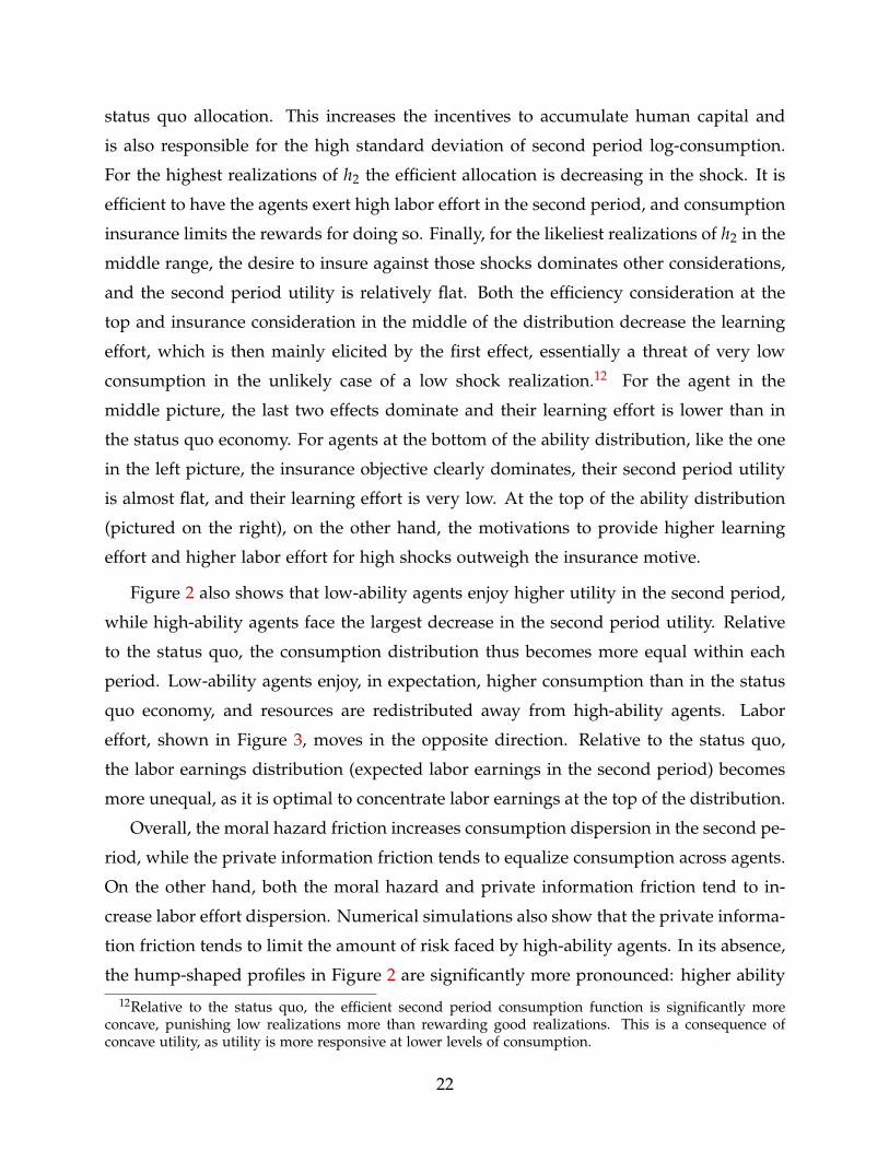
quo economy, and resources are redistributed away from high-ability agents. Labor

effort, shown in Figure 3, moves in the opposite direction. Relative to the status quo,

the labor earnings distribution (expected labor earnings in the second period) becomes

more unequal, as it is optimal to concentrate labor earnings at the top of the distribution.

Overall, the moral hazard friction increases consumption dispersion in the second pe-

riod, while the private information friction tends to equalize consumption across agents.

On the other hand, both the moral hazard and private information friction tend to in-

crease labor effort dispersion. Numerical simulations also show that the private informa-

tion friction tends to limit the amount of risk faced by high-ability agents. In its absence,

the hump-shaped profiles in Figure 2 are significantly more pronounced: higher ability12Relative to the status quo, the efficient second period consumption function is significantly more

concave, punishing low realizations more than rewarding good realizations. This is a consequence ofconcave utility, as utility is more responsive at lower levels of consumption.

22

10 50 90 990

0.2

0.4

0.6

0.8

1

1.2

1.4

Ability Percentile

Laborℓ 1

Efficient

Status Quo

(a) First period.

10 50 90 990

0.2

0.4

0.6

0.8

1

1.2

1.4

Ability Percentile

LaborE(ℓ

2)

Efficient

Status Quo

(b) Second period (expected values).

Figure 3: Labor, by ability percentiles.

agents face more left-tail downside risk, but they also face more right-tail downside risk

of having lower utility after receiving high shocks.

Savings wedge. Figure 4 illustrates that the savings wedge is strictly increasing in abil-

ity. Since high-ability agents face the riskiest second period consumption, they have the

highest incentive to self-insure through savings. In order to discourage that, the social

planner imposes a higher savings tax on them. This result stands in contrast to the previ-

ous literature that features exogenous i.i.d. shocks (e.g. Albanesi and Sleet (2006)), where

high-ability agents typically face less consumption risk, and a lower savings wedge than

low-ability agents.

Labor wedge. The labor wedge in the first period and the expected labor wedge in the

second period are shown in Figure 5a. Several features stand out. First, since high-ability

agents are faced with the highest savings tax, they also need the highest increase in the

labor wedge. Hence the difference between the first period labor wedge and the second

period expected labor wedge is highest for high-ability agents (but small, at about 2%

increase). Second, the labor wedge in period 1 decreases with abilities and converges to

zero. This is due to the assumption of lognormally distributed abilities, as in the static

23

10 50 90 990

0.05

0.1

0.15

0.2

0.25

0.3

0.35

Ability Percentile

Inte

rtempora

lW

edge

Figure 4: Savings Wedge

10 50 90 990

0.1

0.2

0.3

0.4

0.5

0.6

0.7

0.8

0.9

1

Ability Percentile

Wedge

Intratemporal wedge, first period

Expected intratemporal wedge,

second period

(a)

1 2 3 4 50

0.1

0.2

0.3

0.4

0.5

0.6

0.7

0.8

0.9

1

Human Capital h 2

Wedge

Low Ability (0%)

Medium Ability (50%)

High Ability (99.9%)

(b)

Figure 5: Labor Wedge

Mirrlees case, and the fact that the utility function is additively separable in labor supply

and effort. The second period labor wedge is shown in Figure 5b. The labor wedge is

very high for low human capital realizations and then decreases with human capital, as

24

predicted in Proposition 3. The decrease is most rapid for higher ability levels, reflecting

the fact that higher ability agents face a more risky consumption profile.

Welfare. We now compute the welfare gains relative to the status quo. The overall

welfare gain is defined as the percentage increase in period consumption that would

make an agent who does not yet know her type indifferent between the status quo

allocation and the constrained efficient allocation, keeping labor and effort unchanged.

Specifically, the welfare gain is the η that solves,

W((1 + η)cSQ

1 , (1 + η)cSQ2 , `SQ

1 , `SQ2 , eSQ

1

)= WCE.

where the SQ denote status quo allocations and CE denotes constrained efficient alloca-

tions. We find that the welfare gains of switching to an optimal tax system are equivalent

to a η = 4.5% increase in consumption in every period and state of the world.

Table 3: Welfare Gains

Welfare Gains

Status Quo 0%Constrained Efficient 4.5%No moral hazard 6.4%No private information 26.8%No frictions 32.7%

We report the welfare gains in Table 3. Shutting down the moral hazard friction com-

pletely (by setting the Lagrange multiplier φ(a) = 0) yields welfare gains of 6.4% over

the status quo. Shutting down the private information friction completely (by setting the

Lagrange multiplier θ(a) = 0) yields a much larger gain in welfare of 26.8%. Shutting

down both constraints completely yields a first-best welfare gain of 32.7%.

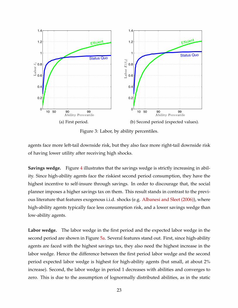
The distribution of welfare changes across types is illustrated in Figure 6. The large

welfare gains accrue at the bottom of the ability distribution. In contrast, the top abilities

lose a substantial amount of welfare compared to the status quo economy. However, it is

worth noting that welfare is increasing with ability in the constrained efficient economy.

Recall that welfare must be increasing with ability level in order to prevent agents from

misreporting their ability level, as expressed by the envelope condition (9).

25

1% 16% 50% 84% 99%−60

−40

−20

0

20

40

60

Ability Percentile

%W

elfare

Change

Figure 6: Welfare change of the unborn agent, from the status quo to the constrainedefficient economy, by ability percentiles.

4.3 Verifying the validity of the First Order Approach

Since second period utility is not monotonically increasing in human capital realizations,

as shown in Figure 2, the sufficient conditions in Proposition 6 are not satisfied. We

therefore verified directly that the expected lifetime utility is concave in the effort. Figure

7 shows that this is indeed the case, and that the first order approach is valid.

5 Conclusion

This paper addresses two questions: What is the optimal tax structure when there is

endogenous human capital accumulation? What are the welfare gains for the U.S. from

switching to an optimal tax system? We answer these normative questions in a hu-

man capital framework that has been successful at positive analysis. The prominent

features of the framework are permanent ability differences, Ben-Porath human capital

accumulation technology, and risky returns to investments in human capital. The model

is sufficiently rich to be useful for policy analysis, and we show that it is also tractable

enough for the normative analysis.

26

0 0.2 0.4 0.6 0.8 1−1

−0.8

−0.6

−0.4

−0.2

0

0.2

0.4

Effort e1

LifetimeUtility

99% ability97%84%

50%

16%

1% ability

Figure 7: Verification of concavity of effort decision

We highlight five main findings. First, it is efficient to design the tax system so that

higher ability people face higher consumption risk in order to provide them with incen-

tives to accumulate human capital. Second, we provide a sharp characterization of the

labor wedge. Under certain conditions, the average intratemporal wedge is increasing

over an agent’s lifetime in order to correct for undesired distortions from the savings

tax. Third, the “no distortion at the top” result from Mirrlees (1971) might not apply

when taxing labor encourages human capital accumulation. Fourth, the savings wedge

is increasing in ability. Finally, we find that there are large welfare gains from switching

to an optimal tax system in the benchmark.

We have assumed that human capital investments are completely unobservable. While

this is more likely the case for older workers who have completed their formal education,

human capital investments earlier in life have a significant observable component, such

as schooling hours. It would be interesting to explore how incentives to elicit unobserv-

able human capital investments interact with schooling subsidies and other incentives to

elicit observable human capital investments.

27

Appendix A A Lagrangean Solution Method

Let λ, φ(a)q(a) and θ(a)q(a) be the Lagrange multipliers on the resource constraint (6),

the first order condition (8) and on the envelope condition (9). The planning problem

can be written as a saddle point of the Lagrangean

maxc,y,e

minλ,θ,φL,

where

L =∫

A

{(1 + θ(a)

)W(a)− θ(a)W(a)

− λ

[c1(a)− y1(a) + β

∫H[c2(a, h2)− y2(a, h2)] p(h2|e1(a)) dh2

]− θ(a)

∫ a

a

[V`

(y1(a)ah1

, e1(a))

y1(a)ah1

+ β∫

HV`

(y2(a, h2)

ah2, 0)

y2(a, h2)

ah2p(h2|e1(a)) dh2

]daa

− φ(a)[

Ve

(y1(a)ah1

, e1(a))− β

∫H

[U(c2(a, h2))−V

(y2(a, h2)

ah2, 0)]

pe(h2|e1(a)) dh2

]}q(a) da

The first-order condition in W(a) implies∫

A θ(a)q(a) da = 0. Using this, integrating by

parts and rearranging terms, one obtains

L =∫

A

{(1 + θ(a)

)W(a)− λ

[c1(a)− y1(a) + β

∫H[c2(a, h2)− y2(a, h2)] p(h2|e1(a)) dh2

]−Θ(a)

[V`

(y1(a)ah1

, e1(a))

y1(a)ah1

+ β∫

HV`

(y2(a, h2)

ah2, 0)

y2(a, h2)

ah2p(h2|e1(a)) dh2

]− φ(a)

[Ve

(y1(a)ah1

, e1(a))+ β

∫H

[U(c2(a, h2))−V

(y2(a, h2)

ah2, 0)]

pe(h2|e1(a))p(h2|e1(a))

p(h2|e1(a)) dh2

]}q(a) da

where Θ(a) = (aq(a))−1∫ a

a θ(a)q(a) da is the cross-sectional cumulative of the Lagrange

multipliers on the envelope condition.

Appendix B Implementation

In this section we decentralize the efficient allocations through a tax system. We describe

the tax system in two steps. In the first one, we follow Werning (2011) to augment the

28

direct mechanism and allow the agents to borrow and save, but design the savings tax in

such a way that the agents choose not to do so. In the second step, we design an indirect

tax mechanism that implements the efficient allocation.

Step 1. In the first step, define the tax on savings as follows. Suppose that an a-type

agent reports a. Enlarge the direct mechanism by allowing the agent to borrow and save.

Let s be pre-tax savings, and x(s) be second period after-tax savings satisfying x(0) = 0.

The agent’s budget constraints are

c1 + s ≤ c1(a) (A-1)

c2 ≤ c2(a, h2) + x(s) ∀h2. (A-2)

x(s) can be easily transformed to a more usual tax on interest income τk(s) by x(s) =[1 + r

(1− τk(s)

)]s. Let the lifetime utility from the utility-maximizing report, condi-

tional on savings being s be

W(s; x|a) = maxa

{U(c1(a)− s)−V

(y1(a)ah1

, e)

+ β∫

H

[U(c2(a, h2) + x(s))−V

(y2(a, h2)

ah2, 0)]

p(h2|e)dh2

}.

For each ability level a, define now a function x∗(·, a) to be a function x such that the

agent is indifferent among all the savings levels:

W(s; x∗(·, a)|a) = W(a) ∀s.

Differentiating the function x∗ and evaluating at s = 0, one obtains x∗s (0, a) = 1− δ(a)

and x∗a(0, a) = 0. That is, the derivative with respect to the savings is equal to the inverse

of the savings wedge, and the derivative with respect to one’s type is always zero, when

evaluated at zero savings.13

13The second derivative follows simply from the fact that x∗(0, a) = 0 for all a.

29

Step 2. In the second step consider a tax system consisting of income tax functions

T1(y1), T2(y1, y2, h2) and a savings tax X(s, y1) satisfying X(0, y1) = 0. While the first

period income tax depends only on the current income, the second period income tax

depends on the second period human capital realization, and can potentially depend on

the history of incomes. The agent faces the following budget constraints:

c1 + s ≤ y1 − T1(y1) (A-3)

c2 ≤ X(s, y1) + y2 − T2(y1, y2, h2) ∀h2. (A-4)

A consumer with ability a maximizes the expected utility

U(c1)−V(

y1

ah1, e)+ β

∫H

[U(c2(h2))−V

(y2(h2)

ah2, 0)]

p(h2|e)dh2 (A-5)

subject to the budget constraints (A-3) and (A-4). The solution to this market problem for

all abilities is given by (c, y, s), where (c, y) is an allocation and s(a) are savings. We

prove the following version of the taxation principle (see Hammond (1979)):

Proposition 8. If an allocation (c, y) satisfies the incentive constraint (5) then there exists a

tax system (T1, T2, X) such that X(0, y) = 0 for all y, and (c, y, 0) solves the market problem.

Conversely, let (T1, T2, X) be a tax system such and (c, y, 0) solves the market problem. Then the

allocation (c, y) is incentive compatible.

Proof. Suppose that an allocation (c, y) satisfies the incentive constraint (5). Define the tax

functions (T1, T2, X) to be such that they satisfy

T1 (y1(a)) = c1(a)− y1(a)

T2 (y1(a), y2(a, h2), h2) = c2(a, h2)− y2(a, h2)

X(s, y1(a)) = x∗(s, a).

For other values in the domain set the taxes T1 and T2 high enough so that no agent chooses such

values. Let

W(s, a|a) = U (c1(a)− s)−V(

y1(a)ah1

, e)

+ β∫

H

[U (c2(a, h2) + x∗(s))−V

(y2(a, h2)

ah2, 0)]

p(h2|e) dh2.

30

Note that W(s; x∗|a) = maxa W(s, a|a). By the definition of x∗,

W(a|a) = W(0, a|a) ≥ maxs

W(s, a|a) ≥ W(0, a|a) = W(a|a) ∀a ∈ A,

Choosing (c, y, 0) yields lifetime utility W(a|a). Any other choice yields W(s, a|a) or lower. Hence

(c, y, 0) solves the market problem.

Conversely, take any tax system (T1, T2, M), and let (c, y, s) be the solution to the market

problem. Then a type a agent prefers (c(a), y(a), 0) to (c(a), y(a), 0). The allocation (c, y) is thus

incentive compatible.

References

Abraham, A., S. Koehne, and N. Pavoni (2012). Optimal income taxation with asset

accumulation. Working paper. 5

Aguiar, M. and E. Hurst (2013). Deconstructing life-cycle expenditure. Journal of Polit-

ical Economy 121(3), 437 – 492. 4

Albanesi, S. (2007). Optimal taxation of entrepreneurial capital with private informa-

tion. Working paper, Columbia University. 5

Albanesi, S. and C. Sleet (2006). Dynamic optimal taxation with private information.

The Review of Economic Studies 73(1), 1–30. 3, 4, 23

Battaglini, M. and S. Coate (2008). Pareto efficient income taxation with stochastic

abilities. Journal of Public Economics 92(3-4), 844–868. 4

Ben-Porath, Y. (1967). The production of human capital and the life cycle of earnings.

Journal of Political Economy 75(4), pp. 352–365. 4

Bohácek, R. and M. Kapicka (2008). Optimal human capital policies. Journal of Mone-

tary Economics 55, 1–16. 3, 5

Browning, M., L. P. Hansen, and J. J. Heckman (1999). Micro data and general equi-

librium models. In M. Woodford and J. Taylor (Eds.), Handbook of Macroeconomics,

Volume 1, Chapter 8. North Holland. 17, 18

Chetty, R., A. Guren, D. Manoli, and A. Weber (2011, May). Are micro and macro labor

31

supply elasticities consistent? a review of evidence on the intensive and extensive

margins. American Economic Review 101(3), 471–75. 17, 18

da Costa, C. E. and L. J. Maestri (2007). The risk properties of human capital and the

design of government policies. European Economic Review 51(3), 695 – 713. 5

Diamond, P. and J. Mirrlees (2002). Optimal taxation and the le chatelier principle.

Working paper, MIT. 5

Farhi, E. and I. Werning (2005). Inequality and social discounting. Journal of Political

Economy 115(1), 365–402. 4

Farhi, E. and I. Werning (2013). Insurance and taxation over the life cycle. The Review

of Economic Studies 80(2), 596–635. 4

Findeisen, S. and D. Sachs (2013). Education and optimal dynamic taxation: The role

of income-contingent student loans. Working paper, University of Mannheim. 5

Findeisen, S. and D. Sachs (2014). Designing efficient college and tax policies. Working

paper, University of Mannheim. 5

Golosov, M., N. R. Kocherlakota, and A. Tsyvinski (2003). Optimal indirect and capital

taxation. The Review of Economic Studies 70, 569–587. 4

Golosov, M., A. Tsyvinski, and M. Troshkin (2015). Redistribution and social insur-

ance. Working paper, Yale University. 4

Gorry, A. and E. Oberfield (2012, October). Optimal taxation over the life cycle. Review

of Economic Dynamics 15(4), 551–572. 5

Grochulski, B. and T. Piskorski (2010). Risky human capital and deferred capital in-

come taxation. Journal of Economic Theory 145(3), 908 – 943. 5, 13

Guner, N., R. Kaygusuz, and G. Ventura (2014, October). Income Taxation of U.S.

Households: Facts and Parametric Estimates. Review of Economic Dynamics 17(4),

559–581. 17, 19

Guvenen, F. (2007). Learning your earning: Are labor income shocks really very per-

sistent? American Economic Review 97(3), 687–712. 4

Hammond, P. J. (1979). Straightforward individual incentive compatibility in large

economies. The Review of Economic Studies 46, 263–282. 30

32

Huggett, M., G. Ventura, and A. Yaron (2006). Human capital and earnings distribu-

tion dynamics. Journal of Monetary Economics 53, 265–290. 4, 19

Huggett, M., G. Ventura, and A. Yaron (2011). Sources of lifetime inequality. American

Economic Review 101(7), 2923–54. 2, 4, 7, 17, 18, 19, 20

Jacobson, L. S., R. J. LaLonde, and D. G. Sullivan (1993, September). Earnings losses

of displaced workers. American Economic Review 83(4), 685–709. 7

Jewitt, I. (1988). Justifying the first-order approach to principal-agent problems. Econo-

metrica 56(5), pp. 1177–1190. 15, 16

Kambourov, G. and I. Manovskii (2009, 02). Occupational specificity of human capital.

International Economic Review 50(1), 63–115. 7

Kapicka, M. (2006). Optimal taxation and human capital accumulation. Review of Eco-

nomic Dynamics 9, 612–639. 5

Kapicka, M. (2015). Optimal mirrleesean taxation with unobservable human capital

formation. AEJ: Macroeconomics, forthcoming. 3, 5, 13

Kocherlakota, N. R. (2005). Zero expected wealth taxes: A Mirrless approach to dy-

namic optimal taxation. Econometrica 73, 1587–1621. 4

Krueger, D. and A. Ludwig (2013, January). Optimal progressive taxation and ed-

ucation subsidies in a model of endogenous human capital formation. American

Economic Review P&P 103, 496–501. 5

Lillard, L. A. and Y. Weiss (1979). Components of variation in panel earnings data:

American scientists 1960-70. Econometrica 47, 437–453. 4

MaCurdy, T. (1982). The use of time-series processes to model the er- ror structure of

earnings in a longitudinal data analysis. Journal of Econometrics, 18, 83–114. 4

McDaniel, C. (2007). Average tax rates on consumption, investment, labor and capital

in the oecd 1950-2003. Working paper, Arizona State University. 17, 19

Mirrlees, J. A. (1971). An exploration in the theory of optimum income taxation. The

Review of Economic Studies 38, 175–208. 4, 12, 27

Mirrlees, J. A. (1976). Optimal tax theory: A synthesis. Journal of Public Economics 6,

327–358. 4

33

Neal, D. (1995). Industry-specific human capital: Evidence from displaced workers.

Journal of Labor Economics 13(4), pp. 653–677. 7

Parent, D. (2000). Industry-specific capital and the wage profile: Evidence from the

national longitudinal survey of youth and the panel study of income dynamics.

Journal of Labor Economics 18(2), pp. 306–323. 7

Peterman, W. B. (2012). The effect of endogenous human capital accumulation on

optimal taxation. Finance and Economics Discussion Series 2012-03, Board of Gov-

ernors of the Federal Reserve System (U.S.). 5, 14

Poletaev, M. and C. Robinson (2008, 07). Human capital specificity: Evidence from the

dictionary of occupational titles and displaced worker surveys, 1984-2000. Journal

of Labor Economics 26(3), 387–420. 7

Primiceri, G. E. and T. van Rens (2009). Heterogeneous life-cycle profiles, income risk

and consumption inequality. Journal of Monetary Economics 56, 20–39. 4

Saez, E. (2001). Using elasticities to derive optimal income tax rates. The Review of

Economic Studies 68, 205–229. 14

Shourideh, A. (2011). Optimal taxation of wealthy individuals. Working paper, Uni-

versity of Minnesota. 5

Slavík, C. and H. Yazici (2014). Machines, buildings, and optimal dynamic taxes. Jour-

nal of Monetary Economics 66(0), 47 – 61. 13

Stantcheva, S. (2015a). Learning and (or) doing: Human capital investments and opti-

mal taxation. Working paper, Harvard. 5

Stantcheva, S. (2015b). Optimal taxation and human capital policies over the life cycle.

Working paper, Harvard. 5

Stiglitz, J. E. (1982). Self-selection and pareto efficient taxation. Journal of Public Eco-

nomics 1(2), 213 – 240. 13

Storesletten, K., C. Telmer, and A. Yaron (2004). Consumption and risk sharing over

the life cycle. Journal of Monetary Economics 51, 609–633. 4

Werning, I. (2007). Optimal fiscal policy with redistribution. Quarterly Journal of Eco-

nomics 22(3), 925967. 4

34

Werning, I. (2011). Nonlinear capital taxation. Working paper, MIT. 3, 28

35