Optimal Taxation in Theory and PracticeThe Harvard community has made this

article openly available. Please share howthis access benefits you. Your story matters

Citation Mankiw, N. Gregory, Matthew Charles Weinzierl, and Danny FerrisYagan. 2009. Optimal taxation in theory and practice. Journal ofEconomic Perspectives 23(4): 147-174.

Published Version doi:10.1257/jep.23.4.147

Citable link http://nrs.harvard.edu/urn-3:HUL.InstRepos:4263739

Terms of Use This article was downloaded from Harvard University’s DASHrepository, and is made available under the terms and conditionsapplicable to Open Access Policy Articles, as set forth at http://nrs.harvard.edu/urn-3:HUL.InstRepos:dash.current.terms-of-use#OAP

1

Optimal Taxation in Theory and Practice

N. Gregory Mankiw, Matthew Weinzierl, and Danny Yagan

Abstract: We highlight and explain eight lessons from optimal tax theory and compare them to the last few decades of OECD tax policy. As recommended by theory, top marginal income tax rates have declined, marginal income tax schedules have flattened, redistribution has risen with income inequality, and commodity taxes are more uniform and are typically assessed on final goods. However, trends in capital taxation are mixed, and capital income tax rates remain well above the zero level recommended by theory. Moreover, some of theory's more subtle prescriptions, such as taxes that involve personal characteristics, asset-testing, and history-dependence, remain rare in practice. Where large gaps between theory and policy remain, the difficult question is whether policymakers need to learn more from theorists, or the other way around.

N. Gregory Mankiw is Professor of Economics, Matthew Weinzierl is Assistant Professor of

Business Administration, and Danny Yagan is a Ph.D. candidate in Economics, all at Harvard

University, Cambridge, Massachusetts. Their e-mail addresses are <ngmankiw@harvard.edu>,

<mweinzierl@hbs.edu>, and <yagan@fas.harvard.edu>.

2

The optimal design of a tax system is a topic that has long fascinated economic theorists

and flummoxed economic policymakers. This paper explores the interplay between tax theory

and tax policy. It identifies key lessons policymakers might take from the academic literature on

how taxes ought to be designed, and it discusses the extent to which these lessons are reflected in

actual tax policy.

We begin with a brief overview of how economists think about optimal tax policy, based

largely on the foundational work of Ramsey (1927) and Mirrlees (1971). We then put forward

eight general lessons suggested by optimal tax theory as it has developed in recent decades: 1)

Optimal marginal tax rate schedules depend on the distribution of ability; 2) The optimal

marginal tax schedule could decline at high incomes; 3) A flat tax, with a universal lump-sum

transfer, could be close to optimal; 4) The optimal extent of redistribution rises with wage

inequality; 5) Taxes should depend on personal characteristics as well as income; 6) Only final

goods ought to be taxed, and typically they ought to be taxed uniformly; 7) Capital income ought

to be untaxed, at least in expectation; and 8) In stochastic, dynamic economies, optimal tax

policy requires increased sophistication. For each lesson, we discuss its theoretical underpinnings

and the extent to which it is consistent with actual tax policy.

To preview our conclusions, we find that there has been considerable change in the

theory and practice of taxation over the past several decades—although the two paths have been

far from parallel. Overall, tax policy has moved in the directions suggested by theory along a

few dimensions, even though the recommendations of theory along these dimensions are not

always definitive. In particular, among OECD countries, top marginal rates have declined,

marginal income tax schedules have flattened, and commodity taxes are more uniform and are

typically assessed on final goods. However, trends in capital taxation are mixed, and rates still

are well above the zero level recommended by theory. Moreover, some of theory’s more subtle

prescriptions, such as taxes that involve personal characteristics, asset-testing, and history-

dependence, remain rare. Where large gaps between theory and policy remain, the harder

question is whether policymakers need to learn more from theorists, or the other way around.

Both possibilities have historical precedents.

The Theory of Optimal Taxation

3

The standard theory of optimal taxation posits that a tax system should be chosen to

maximize a social welfare function subject to a set of constraints. The literature on optimal

taxation typically treats the social planner as a utilitarian: that is, the social welfare function is

based on the utilities of individuals in the society. In its most general analyses, this literature uses

a social welfare function that is a nonlinear function of individual utilities. Nonlinearity allows

for a social planner who prefers, for example, more equal distributions of utility. However, some

studies in this literature assume that the social planner cares solely about average utility,

implying a social welfare function that is linear in individual utilities. For our purposes in this

essay, these differences are of secondary importance, and one would not go far wrong in thinking

of the social planner as a classic “linear” utilitarian.1

To simplify the problem facing the social planner, it is often assumed that everyone in

society has the same preferences over, say, consumption and leisure. Sometimes this

homogeneity assumption is taken one step further by assuming the economy is populated by

completely identical individuals. The social planner’s goal is to choose the tax system that

maximizes the representative consumer’s welfare, knowing that the consumer will respond to

whatever incentives the tax system provides. In some studies of taxation, assuming a

representative consumer may be a useful simplification. However, as we will see, drawing

policy conclusions from a model with a representative consumer can also in some cases lead to

trouble.

After determining an objective function, the next step is to specify the constraints that the

social planner faces in setting up a tax system. In a major early contribution, Frank Ramsey

(1927) suggested one line of attack: suppose the planner must raise a given amount of tax

revenue through taxes on commodities only. Ramsey showed that such taxes should be imposed

in inverse proportion to the representative consumer’s elasticity of demand for the good, so that

commodities which experience inelastic demand are taxed more heavily. Ramsey’s efforts have

had a profound impact on tax theory as well as other fields such as public goods pricing and

1 Stiglitz (1987) addressed the more restricted agenda of identifying Pareto-efficient taxation, an approach taken up recently by Werning (2007). This approach is important because it suggests that many of the general prescriptions of the optimal taxation models that use utilitarian social welfare functions survive being recast in Pareto terms, which in turn suggests that the precise form of the social welfare function (at least in the class of all Pareto functions) is not very important for some findings. Despite the more solid normative ground on which this approach rests, it so far has had less influence in the development of tax theory than the utilitarian approach of Mirrlees (1971).

4

regulation. However, from the standpoint of the optimal taxation literature, in which the goal is

to derive the best tax system, it is obviously problematic to rule out some conceivable tax

systems by assumption. Why not allow the social planner to consider all possible tax schemes,

including nonlinear and interdependent taxes on goods, income from various sources, and even

non-economic personal characteristics?

But if the social planner is allowed to be unconstrained in choosing a tax system, then the

problem of optimal taxation becomes too easy: the optimal tax is simply a lump-sum tax. After

all, if the economy is described by a representative consumer, that consumer is going to pay the

entire tax bill of the government in one form or another. Absent any market imperfection such as

a preexisting externality, it is best not to distort the choices of that consumer at all. A lump-sum

tax accomplishes exactly what the social planner wants.

In the world, there are good reasons why lump-sum taxes are rarely used. Most

important, this tax falls equally on the rich and poor, placing a greater relative burden on the

latter. When Margaret Thatcher, during her time as the Prime Minister of the United Kingdom,

successfully pushed through a lump-sum tax levied at the local level (a “community charge”)

beginning in 1989, the tax was deeply unpopular. As the New York Times reported in 1990,

“[W]idespread anger over the tax threatens Mrs. Thatcher's political life, if not her physical

safety. And it may prove to be the last hurrah for her philosophy of public finance, in which the

goals of efficiency and accountability take precedence over the values of the welfare state”

(Passell, 1990). The tax was quickly revoked, and not coincidentally, Thatcher’s term of office

ended not long after.

As this episode suggests, the social planner has to come to grips with heterogeneity in

taxpayers’ ability to pay. If the planner could observe differences among taxpayers in inherent

ability, the planner could again rely on lump-sum taxes, but now those lump-sum taxes would be

contingent on ability. These taxes would not depend on any choice an individual makes, so it

would not distort incentives, and the planner could achieve equality with no efficiency costs.2

2 In this case, the optimal policy may yield surprising results. For example, with additively separable utility, once the tax system is in place, the high-ability individuals typically have lower utility than low-ability individuals. Because of diminishing marginal utility, the social planner equalizes consumption of high- and low-ability taxpayers. But it is optimal for the high-ability taxpayers to work more and enjoy less leisure. The planner uses the targeted lump-sum tax to redistribute the product of their additional effort.

5

Actual governments, however, cannot directly observe ability, so the model still fails to deliver

useful and realistic prescriptions.

James Mirrlees (1971) launched the second wave of optimal tax models by suggesting a

way to formalize the planner’s problem that deals explicitly with unobserved heterogeneity

among taxpayers. In the most basic version of the model, individuals differ in their innate ability

to earn income. The planner can observe income, which depends on both ability and effort, but

the planner can observe neither ability nor effort directly. If the planner taxes income in an

attempt to tax those of high ability, individuals will be discouraged from exerting as much effort

to earn that income. By recognizing unobserved heterogeneity, diminishing marginal utility of

consumption, and incentive effects, the Mirrlees approach formalizes the classic tradeoff

between equality and efficiency that real governments face, and it has become the dominant

approach for tax theorists.

In the Mirrlees framework, the optimal tax problem becomes a game of imperfect

information between taxpayers and the social planner. The planner would like to tax those of

high ability and give transfers to those of low ability, but the social planner needs to make sure

that the tax system does not induce those of high ability to feign being of low ability. Indeed,

modern Mirrleesian analysis often relies on the “revelation principle.” According to this classic

game theoretic result, any optimal allocation of resources can be achieved through a policy under

which individuals voluntarily reveal their types in response to the incentives provided.3 In other

words, the social planner has to make sure the tax system provides sufficient incentive for high-

ability taxpayers to keep producing at the high levels that correspond to their ability, even though

the social planner would like to target this group with higher taxes.

The strength of the Mirrlees framework is that it allows the social planner to consider all

feasible tax systems. The weakness of the Mirrlees approach is its high level of complexity.

Keeping track of the incentive-compatibility constraints required so that individuals do not

produce as if they had lower levels of ability makes the optimal tax problem much harder.

Since the initial Mirrlees contribution, however, much progress has been made using this

approach. General treatments of the Mirrlees approach are found in Tuomala (1990), Salanie

(2003), and Kaplow (2008a).

3 Optimal tax research in the spirit of Mirrlees (1971) has generally avoided situations in which the Revelation Principle does not apply, such as if the social planner cannot commit to a future policy plan.

6

In the rest of this paper, we focus on eight of the most prominent lessons suggested by

optimal tax theory. Many of these were first derived in work during the 1970s and 1980s, and

part of this paper’s goal is to update readers on more recent work that has built on or qualified,

sometimes substantially, these results. For each lesson, we lay out the intuition and then examine

data to see whether recent tax policy has moved in the recommended direction.

Lesson 1: Optimal Marginal Tax Rate Schedules Depend On The Distribution Of Ability

A primary focus of modern optimal tax research has been the schedule of marginal tax

rates on labor income. This was the heart of Mirrlees' (1971) contribution, and it remained a

high-profile topic of research—at least until recent work in dynamic models discussed later.

In the Mirrlees model, the schedule of marginal tax rates is the main battleground in the

tradeoff between equality and efficiency. Consider an increase in the marginal tax rate at a given

level of income. This tax hike has an efficiency cost because it discourages the individuals who

earn that income from exerting effort. But the tax change is nondistortionary for individuals who

earn higher incomes. It raises their average tax rate, but not their marginal tax rate. Because this

tax hike raises revenue from the upper part of the income distribution and can be used to finance

transfers to all individuals, it can yield an equality benefit. These factors suggest a cost-benefit

analysis that applies to any proposal to alter the schedule of marginal tax rates. Other things

equal, an increase in a marginal tax rate is more attractive when few individuals would be

affected at the margin and many would be affected inframarginally. Therefore, to strike the right

balance between efficiency and equality, the marginal tax rate schedule must be tailored to the

shape of the ability distribution.

By itself, this lesson is too broad and nonspecific to be of direct help to practical

policymakers. But it lays a foundation for the next few lessons.

Lesson 2: The Optimal Marginal Tax Schedule Could Decline At High Incomes

7

How high should marginal tax rates be for high-income workers? Wide variation in top

marginal rates across time and countries suggests substantial uncertainty, or at least fluctuation,

in policymakers’ answers to this question. Before turning to the data, we examine the answer

from optimal tax theory.

Theory

A well-known early result of the Mirrlees (1971) model is the optimality of a zero top

marginal tax rate. Recent work has undermined the practical relevance of this finding, but the

intuition behind it may still have important implications for the taxation of high earners.

The original Mirrlees argument runs as follows. Suppose there is a positive marginal tax

rate on the individual earning the top income in an economy, and suppose that income is y. The

positive marginal tax rate has a discouraging effect on the individual's effort, generating an

efficiency cost. If the marginal tax rate on that earner was reduced to zero for any income

beyond y, then the same amount of revenue would be collected and the efficiency costs would be

avoided. Thus, a positive marginal tax on the top earner cannot be optimal.

This result, which has been called "striking and controversial" (Tuomala, 1990), is often

discounted as of limited practical relevance. Strictly speaking, this result applies only to a single

person at the very top of the income distribution, suggesting it might be a mere theoretical

curiosity. The potential to redistribute from the highest earner to the population as a whole may

justify large marginal rates on the second-highest earner and other high-ability taxpayers.

Whether it does depends on the shape of the high end of the ability distribution. Moreover, it is

unclear that a "top earner" even exists. For example, Saez (2001) argues that "unbounded

distributions are of much more interest than bounded distributions to address the high income

optimal tax rate problem." Without a top earner, the intuition for the zero top marginal rate does

not apply, and marginal rates near the top of the income distribution may be positive and even

large.

Nonetheless, the intuition behind the zero top rate result suggests that an important task

for policy analysis is to identify the shape of the high end of the ability distribution. In early

numerical simulations of the Mirrlees model, Tuomala (1990) finds, "it will be seen that in all

cases reported ... the marginal tax rate falls as income increases except at income levels within

the bottom decile." In Tuomala's simulations, the efficiency costs of redistribution are large for

8

much of the high end of the income distribution, justifying declining rates for a broad range of

high incomes. These results suggest that the zero top rate result was an instructive, if extreme,

illustration of the power of incentive effects to counteract redistributive motives in setting

marginal rates on high earners. In contrast, Saez (2001), building on the work of Diamond

(1998), also carried out numerical simulations and concluded, in dramatic contrast to earlier

results, that marginal rates should rise between middle- and high-income earners, and that rates

at high incomes should "not be lower than 50% and may be as high as 80%." The primary

difference between these findings seems to reside in the underlying assumptions about the shape

of the distribution of ability. Specifically, Tuomala assumed a lognormal distribution, whereas

Diamond and Saez argued that the right tail is better described by a Pareto distribution, which

has tails thicker than a lognormal.

Estimating the distribution of ability is a task fraught with perils. For example, when

Saez (2001) derives the ability distribution from the observed income distribution, the exercise

requires making assumptions on many topics at and beyond the frontier of the optimal tax

literature. It is unclear to what extent we can rely on this approach’s accuracy.

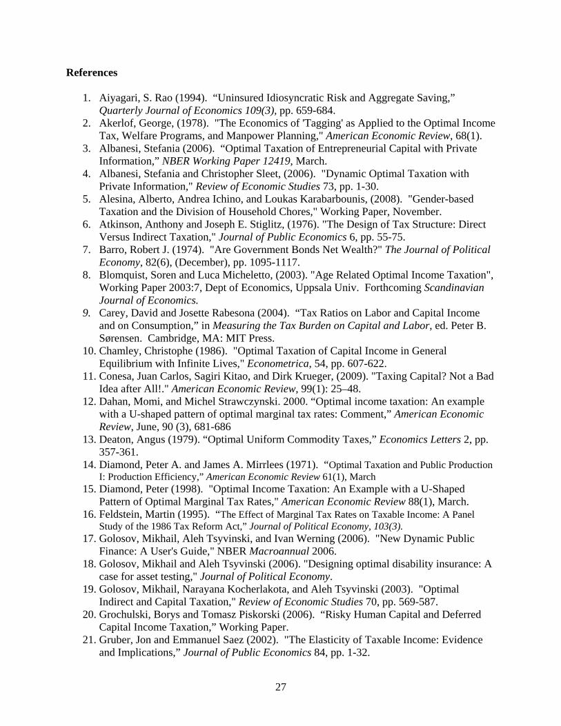
An alternative approach is to use wages as a proxy for ability. Hourly wages, however,

are not a straightforward concept at the top of the income distribution, where labor and capital

income may become intertwined and data on hours worked may not be reliable. Moreover,

available data on wages do not give a clear answer. Using the Current Population Survey rotating

March sample, Figure 1 presents the distribution of wages for individuals earning more than $43

per hour (corresponding to approximately $100,000 annually) and less than $200,000 (to avoid

top-coding). Also shown are two parametric distributions fitted to these data, a lognormal

distribution and a Pareto distribution. As is apparent from the figure, the Pareto and lognormal

fits are virtually indistinguishable over this wage range. Confidential CPS data on the U.S. wage

tail above the level shown in Figure 1 are not publicly available.

Even if the shape of the ability distribution were known, other uncertainties remain. For

example, the question of what appropriate social welfare function to use—and in particular how

much concern there should be over inequality—is a normative question that cannot be answered

with data. In addition, characteristics of the individual’s utility function can affect the pattern of

optimal income tax rates. Dahan and Strawczynski (2000) study the importance of income

effects (equivalently, declining marginal utility of consumption) for the pattern of marginal tax

9

rates. They argue that concave utility lowers optimal tax rates at high incomes and that marginal

tax rates may be declining even for a Pareto distribution of wages. Sandmo (1993), Judd and Su

(2006), Kaplow (2008c), and Weinzierl (2009), among others, study the implications of

interpersonal heterogeneity along dimensions other than ability, such as preferences for

consumption and leisure. They find that additional dimensions of heterogeneity tend to reduce

the optimal extent of redistribution. Finally, the relevant elasticities are crucial for optimal

marginal tax rates. While optimal tax simulations often assume a uniform elasticity, Feldstein

(1995) estimated large elasticities of taxable income with respect to tax rates among high

earners. Gruber and Saez (2002) subsequently estimated smaller elasticities, but their estimates

also support the hypothesis that the elasticity increases with income. If high-income workers are

particularly elastic in how their taxable income decreases with higher tax rates, this would imply

lower optimal marginal tax rates on high incomes, all else the same. But as with the distribution

of abilities and the social welfare function, there is much debate over the true pattern of

elasticities by income.

All this leaves the policy advisor in an uncomfortable position. Early work, following

Mirrlees (1971), assumed a shape for the ability distribution, social welfare and individual utility

functions, and a pattern of labor supply elasticities that yielded clear but surprising results—

declining marginal tax rates at the top of income distribution. Some recent work has yielded

dramatically different results more consistent with existing policy, but many of the key

assumptions are open to debate.

Practice

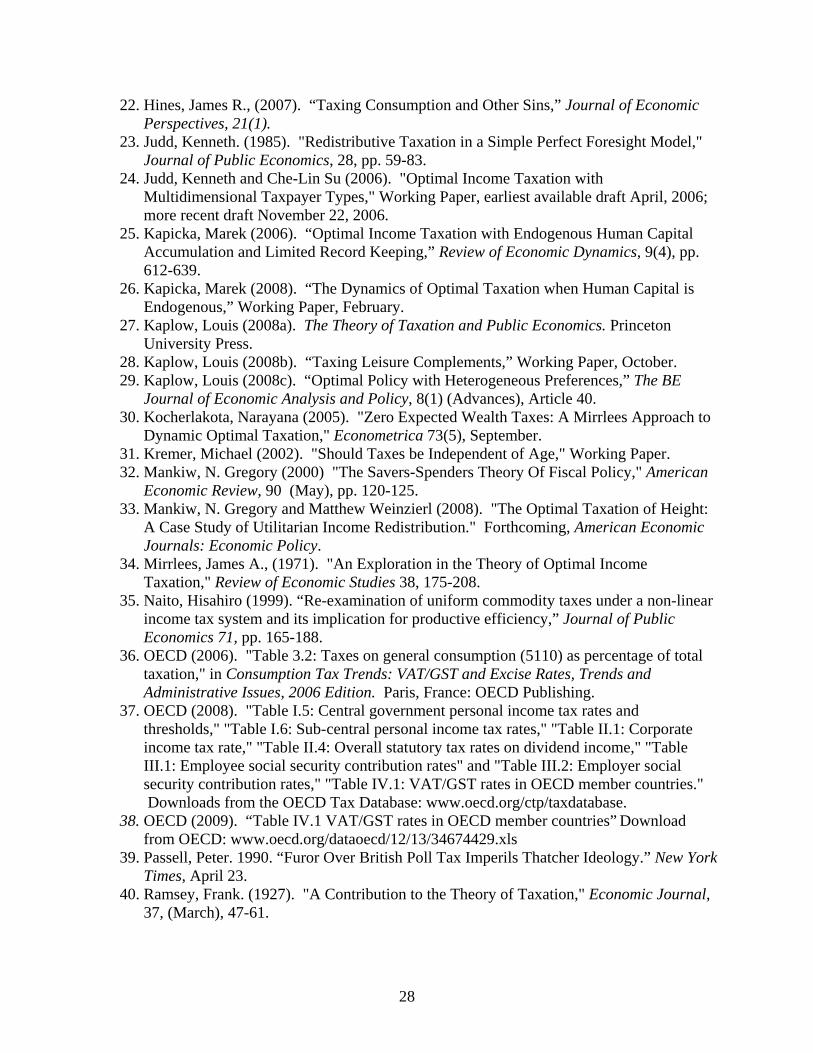
Despite the ambiguity of economic theory, public policy over the last three decades has

steadily moved toward lower marginal tax rates on high earners. Figure 2 shows the top marginal

tax wedge, which combines the top marginal income tax rate with the rate of value-added tax (or

general sales tax) for OECD countries from 1983 to 2007. The average top marginal tax wedge

in OECD countries has fallen steadily over this period, from nearly 80 percent to just above 60

percent. Most of this decline is due to a decline in top marginal income tax rates assessed by the

central government, which have fallen to just above 50 percent over this period. Sub-central and

10

payroll tax rates have remained essentially flat, while value-added and general sales taxes have

increased somewhat.

The very top marginal rate shown in Figure 2, however, may be misleading because it

tells us nothing about the range of incomes over which it applies. For instance, in 2006 the top

marginal rate in the United Kingdom applied to a worker earning 134 percent of the average

employee compensation, while in the United States the corresponding cutoff was 653 percent. If

the minimum income to which top rates apply has fallen over time, then a wider range of high-

income workers are being taxed at a high marginal rate. To take account of this possibility,

Table 1 takes an alternative approach. It shows the top marginal rate assessed on an income that

is 250 percent of average employee compensation in each OECD country where data are readily

available around the endpoints of the period covered in Figure 2: 1981-1982 and 2005-2006.4

The marginal tax rate on high earners has fallen in 11 out of 14 countries, and the few increases

in the rate have been modest. On average, OECD countries have lowered the marginal tax rate at

this high income level by nearly 11 percentage points over the last 25 years.

Lesson 3: A Flat Tax, With A Universal Lump-Sum Transfer, Could Be Close To Optimal

A key determinant of the optimal marginal tax schedule is the shape of the ability

distribution, as discussed earlier. The shapes assumed in early work on optimal taxation tended

to yield relatively flat marginal tax rates. In fact, Mirrlees (1971) wrote: “Perhaps the most

striking feature of the results is the closeness to linearity of the tax schedules.” By linearity,

Mirrlees (and the subsequent literature) is referring to a tax system in which the same marginal

tax rate applies at every income level. Usually, the optimal system combines a flat marginal tax

rate with a lump-sum grant to all individuals, so the average tax rate rises with income even as

the marginal tax rate does not. Here, we examine the debate over that finding.

Theory 4The OECD Tax Database is the broadest and most consistent dataset on income taxes in developed countries. That said, it is imperfect. For example, it appears to include rates on non-labor income for the United States in 1981, raising the reported top marginal rate above 70 percent in that year. We have retained the OECD data as is unless noted otherwise, for transparency. Correcting the U.S. data in 1981 does not significantly affect any of the paper’s discussion. However, for Table 1 we did correct the OECD’s figure for the United States in 1981.

11

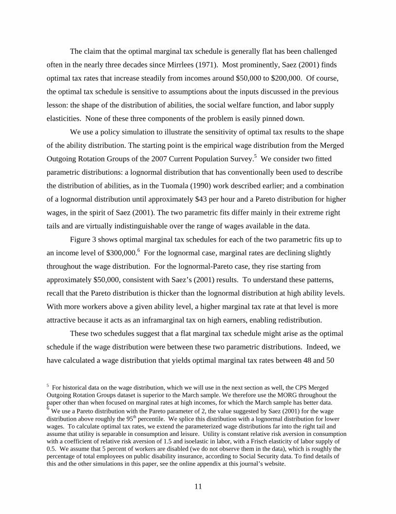
The claim that the optimal marginal tax schedule is generally flat has been challenged

often in the nearly three decades since Mirrlees (1971). Most prominently, Saez (2001) finds

optimal tax rates that increase steadily from incomes around $50,000 to $200,000. Of course,

the optimal tax schedule is sensitive to assumptions about the inputs discussed in the previous

lesson: the shape of the distribution of abilities, the social welfare function, and labor supply

elasticities. None of these three components of the problem is easily pinned down.

We use a policy simulation to illustrate the sensitivity of optimal tax results to the shape

of the ability distribution. The starting point is the empirical wage distribution from the Merged

Outgoing Rotation Groups of the 2007 Current Population Survey.5 We consider two fitted

parametric distributions: a lognormal distribution that has conventionally been used to describe

the distribution of abilities, as in the Tuomala (1990) work described earlier; and a combination

of a lognormal distribution until approximately $43 per hour and a Pareto distribution for higher

wages, in the spirit of Saez (2001). The two parametric fits differ mainly in their extreme right

tails and are virtually indistinguishable over the range of wages available in the data.

Figure 3 shows optimal marginal tax schedules for each of the two parametric fits up to

an income level of $300,000.6 For the lognormal case, marginal rates are declining slightly

throughout the wage distribution. For the lognormal-Pareto case, they rise starting from

approximately $50,000, consistent with Saez’s (2001) results. To understand these patterns,

recall that the Pareto distribution is thicker than the lognormal distribution at high ability levels.

With more workers above a given ability level, a higher marginal tax rate at that level is more

attractive because it acts as an inframarginal tax on high earners, enabling redistribution.

These two schedules suggest that a flat marginal tax schedule might arise as the optimal

schedule if the wage distribution were between these two parametric distributions. Indeed, we

have calculated a wage distribution that yields optimal marginal tax rates between 48 and 50

5 For historical data on the wage distribution, which we will use in the next section as well, the CPS Merged Outgoing Rotation Groups dataset is superior to the March sample. We therefore use the MORG throughout the paper other than when focused on marginal rates at high incomes, for which the March sample has better data. 6 We use a Pareto distribution with the Pareto parameter of 2, the value suggested by Saez (2001) for the wage distribution above roughly the 95th percentile. We splice this distribution with a lognormal distribution for lower wages. To calculate optimal tax rates, we extend the parameterized wage distributions far into the right tail and assume that utility is separable in consumption and leisure. Utility is constant relative risk aversion in consumption with a coefficient of relative risk aversion of 1.5 and isoelastic in labor, with a Frisch elasticity of labor supply of 0.5. We assume that 5 percent of workers are disabled (we do not observe them in the data), which is roughly the percentage of total employees on public disability insurance, according to Social Security data. To find details of this and the other simulations in this paper, see the online appendix at this journal’s website.

12

percent for all but the lowest- and highest-skilled workers and that lies between the lognormal

and lognormal-Pareto distributions except at low wage levels (where fewer disabled and more

low-skilled workers are required to lower the optimal marginal rates shown in Figure 3) and a

few intermediate wage levels (where it slightly exceeds both distributions). This nearly-flat

optimal tax policy provides a lump-sum grant to the lowest-ability worker equal to just over 60

percent of average income per worker in the economy.

One perhaps counterintuitive result of these kinds of simulations is that they imply that

marginal taxes should be higher at low wages than for most of the rest of the distribution. The

intuition behind this result is that high marginal rates at low incomes allow for large lump-sum

transfers to be given to those of the lowest ability levels without tempting higher-ability workers

to work less and claim those transfers. For higher-ability workers, the net value of marginal

income is too high at low incomes, so they are deterred from working less despite the generous

redistribution offered to those with low ability.7

The lesson is that, from the perspective of a Mirrlees-style model, proposals for a flat tax

are not inherently unreasonable. In part, this verdict is due to the many sources of uncertainty

that make it hard to pin down an optimal marginal tax schedule. But it is also due to the

suggestive evidence that simulations can lead to optimal tax schedules that are near, both in

terms of tax rates and welfare impacts, to a flat marginal tax schedule. If a flat marginal tax

schedule has benefits outside the model, such as administrative simplicity, enforceability, and

transparency, the case for it is strengthened.

Practice

Though the optimal tax literature has not conclusively answered the question of how far

from flat is the optimal tax policy, policymakers seem to have decided that flatter is better.

To gauge the flatness of marginal tax schedules, we measure the slopes of the statutory

marginal tax rate schedules for OECD countries from 1981 to 2006. First, we calculate the

7 An important qualification to this result was analyzed by Saez (2002a), who showed that the optimal marginal distortions on low incomes are less, and perhaps even negative at the bottom, if the labor force participation decision is more elastic than the decision about how much effort to supply. However, even in this case, those incentives are taxed away as income rises, much as are the lump-sum grants in the standard analysis. In practice, high marginal tax rates are commonly seen at low incomes, especially in the form of “phase-outs” by which transfer payments are taxed away as income increases.

13

marginal tax rate faced by individuals earning 67, 100, 150, and 250 percent of the average

employee compensation in each country. Then, we calculate the spreads in marginal rates

between those income levels in each year. For instance, the 250-67 spread is the marginal tax

rate on someone who earns 250 percent of the average employee compensation less the marginal

rate on someone who earns 67 percent of the average. These spreads are measures of the slopes

of the tax schedules.

Table 2 shows how the 250-67 spread has changed over the last three decades. Nine of

the 14 countries with available data have moved toward flatter rates, and the average decrease in

the 250-67 spread across these 14 countries was 4.3 percentage points. A similar pattern holds

for the 150-100 spread, which has fallen by over 3 percentage points on average in OECD

countries over this time period. The flat tax has not become the norm among OECD countries,

but many of these nations have moved their tax systems in that direction.

Lesson 4: The Optimal Extent Of Redistribution Rises With Wage Inequality

Economic inequality has risen substantially in recent years, especially in the United

States. From the perspective of the theory of optimal taxation, this change can be seen as a

widening in the distribution of ability. (Labor economists might say that what has changed is the

economic return to ability, not the distribution of innate talent, but the distinction is not crucial

for the matter at hand.) This fact raises an obvious question: How, according to optimal tax

theory, should the social planner respond to such a shift in the economic environment?

Theory

Mirrlees (1971) pointed out that greater inequality in ability makes the optimal tax policy

more redistributive. He suggested that tax rates would generally be higher in less equal societies

and that less of the population would be required to work. Low-ability individuals would enjoy

leisure along with a lump-sum grant to support consumption.

To illustrate this lesson, we simulate optimal tax policy using the observed changes in the

U.S. wage distribution. We begin by taking the data on reported wages from the Merged

Outgoing Rotation Groups of the Current Population Survey for 1979 and 2007. We then

14

calculate the best-fit lognormal distribution to approximate these wages. (Similar results are

obtained for the combination lognormal-Pareto wage distribution.) As one would expect, this

distribution has spread out over the last 30 years, with thicker tails and less mass at average

wages. We treat this distribution of wages as a proxy for ability, and then simulate the

appropriate optimal taxes. Figure 4 shows the simulated optimal average tax schedules using

these two wage distributions. As expected, optimal average tax rates on high earners have

increased. In addition, there is an increase in the transfers made to the low-skilled, visible as the

difference between the left-most points on the two schedules. In an optimal tax model, the

increased earnings potential at the top of the distribution enables more redistribution toward the

low-skilled, so that the increase in earnings inequality does not translate into as great an increase

in disposable income inequality.

Practice

To test whether policy responds to the level of inequality as the optimal tax models

predict, we examine data on earnings inequality from the Luxembourg Income Study and data on

social expenditures as a share of GDP from the OECD, a commonly-used measure of income

redistribution. If the optimal tax model is consistent with policymaking priorities, we would

expect to see policy react to higher earnings inequality by increasing social expenditures as a

share of GDP.

Table 3 shows the relevant data for the 14 countries covered by the Luxembourg Income

Study. Data are available for multiple years from 1979 through 2000 for each country, so we

have 46 observations for 11 countries in total. The third and fourth columns of the table show

the average Gini coefficients of pre-tax and pre-transfer earnings as well as the average levels of

social expenditure as a share of GDP for each country across the observed years. The last two

columns of the table show the results of regressing each country’s time series of social

expenditures as a share of GDP on its time series of Gini coefficients. Nine of the eleven

countries display a positive relationship between these variables, as the model predicts: that is,

years of higher earnings inequality are also years of relatively higher redistribution. Also

reported in the table are the results of a pooled cross-sectional regression that includes all

observations and that controls for country fixed effects. This regression yields a positive and

15

statistically significant relationship between pre-tax inequality and the share of output devoted to

social expenditures. As theory recommends, greater inequality is associated with more

redistribution.

Lesson 5: Optimal Taxes Should Depend On Personal Characteristics As Well As Income

Mirrlees (1971) identified the heart of the problem of tax design to be the tax authority’s

lack of information about individuals’ abilities. He assumed that the tax authority would use

income as the only indicator of ability, but he recognized that many more indicators could be

used: “One might obtain information about a man’s income-earning potential from his apparent

I.Q., the number of his degrees, his address, age or colour; but the natural, and one would

suppose the most reliable, indicator of his income-earning potential is his income.”

Akerlof (1978) soon showed that those other indicators were potentially important, both

theoretically and empirically. He coined the term “tagging” to describe the use of taxes that are

contingent on personal characteristics, and he formally demonstrated that the use of tagging

might improve on an income-based tax system. He also suggested that tagging played a large

role in existing U.S. policy, citing public spending programs for the elderly, the disabled,

children, and other groups.

For tagging to work, however, high-ability individuals cannot pretend to be members of

the tagged group or, at least, the policymaker must make such cheating very costly, such as by

making the process of obtaining benefits cumbersome and time-consuming. Otherwise, the

optimal level of tagging may be negligible or zero. Even if a tag is entirely exogenous, its appeal

as an argument in the tax function depends on the quality of its signal about an individual’s

ability. If the tag is somewhat related to ability, but the correlation only moderately high—that is,

if the tag is “noisy”—then lump-sum taxes on the “high” type will weigh heavily on those

members of the high type who nevertheless have low ability. Intra-type redistribution can offset

this problem, but only by reducing the extent to which the taxes are lump-sum and, therefore, the

benefit of tagging. Finally, tagging has administrative costs that, though perhaps small at first,

might increase quickly with the complexity of a system that used many tags.

The potential power of well-chosen tags, however, is illustrated by two recent studies.

Alesina, Ichino, and Karabarbounis (2008) consider taxes that depend on gender, while Mankiw

16

and Weinzierl (2008) consider height-dependent taxes. In the former, the value of tagging comes

largely from the differences in labor supply elasticities across genders; in the latter it comes

from differences in the levels of ability (as proxied by wages) across height. While Akerlof

(1978) focused on the use of tags to alleviate poverty, these more recent studies highlight a more

extensive role for tagging in an optimal tax system. Tags not only identify the poor; they also

provide additional information to the policymaker, whether about labor supply elasticities or the

distribution of unobserved ability. For example, if a particular demographic group has a very

wide ability distribution relative to other groups, the policymaker can tailor marginal taxes at

each income level to that wider distribution. Theory suggests that any personal characteristic

that is largely exogenous, easy to monitor, and systematically related to ability or preferences

ought to be included as an argument in the optimal tax function. At least in the narrow context of

an optimal tax model, the economic benefits of tagging by gender and height probably

substantially outweigh the likely administrative costs.

Practice

In a few specific and economically significant ways, tagging is widely used in the real

world. Nearly every developed country restricts some tax benefits, special services, and cash

transfers to poor households with young children. In 2003, the OECD estimated public spending

on family benefits to be 2.4 percent of GDP on average among its 24 member countries where

these data were available. In addition, most developed economies provide specific, tagged

support to a few other demographic groups that may be systematically vulnerable to poverty,

such as the disabled and the elderly.

Nevertheless, the theory behind tagging would suggest a much broader application. In

particular, tax schedules ought to vary systematically, the theory tells us, with gender, height,

skin color, physical attractiveness, health, parents’ education, and so on. No modern tax system

has such variation. The exception is age: several countries including Singapore, Australia, and

the United States reduce the tax burden on individuals over 55 and 65 years of age, but separate

treatment of a narrow range of ages near retirement is a relatively mild version of tagging

relative to what the theory would suggest.

Why are some kinds of tagging prominent, while other possible tags are not used?

Optimal tax theory treats all differences between personal characteristics alike, and asks only

17

how such differences are correlated with labor supply elasticities and ability. Societies appear to

be more comfortable, however, using characteristics that arise over the course of the lifecycle

and may directly signal economic disadvantage, such as parenthood, disability, and old age—in

general, characteristics that anyone might potentially experience at some point in their lifetime.

Conversely, society seems less comfortable using characteristics for tagging that are largely

predetermined at birth and whose relationship with ability or preferences is more subtle, such as

gender, skin color, height, and parents’ education.

Consistent with these differences in treatment, certain kinds of tagging may involve costs

that are excluded from a conventional optimal tax analysis. For example, tagging may seem to

violate horizontal equity, the policy design principle that those of like circumstances should be

treated alike. Exactly how “like circumstances” should be defined is left deliberately vague in

this definition, but many believe that two people with similar abilities should pay the same taxes

regardless of their fixed personal characteristics, and that horizontal equity therefore should be

included as an additional constraint in the optimal tax problem. A second example is that the

appeal of tagging relies on the assumption that ability to pay ought to be the basis for taxation,

rather than another criterion such as benefits received. All individuals may benefit from a tax

system that insures against some shocks, such as disability, but tagging based on predetermined

characteristics will be opposed by those who already know they are the “high type.” These

concerns lie outside the standard optimal tax framework, but they may explain the relatively

limited use of tags.

Lesson 6: Only Final Goods Ought To Be Taxed, And Typically They Ought To Be Taxed

Uniformly

While the optimal taxation of labor income remains something of a mystery, two

powerful results have guided intuition about the optimal taxation of goods and services.

Diamond and Mirrlees (1971) suggest that optimal taxes are zero on all intermediate goods.

Atkinson and Stiglitz (1976) suggest that optimal taxes are equal across all final consumption

goods. Exceptions to these benchmark results have been noted. One well-known exception is

for goods that generate externalities and that therefore justify corrective, Pigovian taxes or

subsidies. For more standard goods, differential commodity taxes can be optimal if goods vary

18

in their complementarity with leisure, if these taxes affect the wages paid to workers of different

skills, or if preferences for goods are correlated with individual abilities, as discussed in Kaplow

(2000b), Naito (1999), and Saez (2002b). But the earlier results remain benchmarks because of

the powerful intuitions behind them.

The intuition behind the Diamond and Mirrlees (1971) result regarding intermediate

goods is that, whatever the optimal allocation of final goods, a social planner would ensure that

production of those goods was done as efficiently as possible. The insight of Diamond and

Mirrlees is that the same set of relative prices as would obtain under a social planner can be

achieved by a tax authority in a competitive economy through varying the set of taxes on final

goods. The implication is that optimal taxes can leave the economy on its production frontier.

Maintaining productive efficiency rules out taxes with differential effects across industries,

sectors, or time periods. It generally forbids taxes on intermediate inputs to production because

they distort the allocation of factor inputs. It argues against taxes on corporate accounting profits

because they distort the return to capital for a subset of the economy, encouraging capital to

leave the corporate sector. Finally, it implies no taxation of human and physical capital because

both are used as inputs to future production, so taxing them would put the economy inside its

production frontier.

While the Diamond and Mirrlees (1971) result restricts the set of goods to which taxes

ought to apply, Atkinson and Stiglitz (1976) derived restrictions on the design of the taxes of

final goods. Atkinson and Stiglitz showed that if the utility function is weakly separable in

leisure and all consumption, and if preferences for goods do not depend on ability, the optimal

taxation of final goods is uniform when a fully nonlinear income tax is available.8 This result

emerges because there is no information about unobserved ability in an individual’s consumption

choice that is not also revealed by the individual’s income, and so the income tax can be matched

to ability as desired. In this setting, the intuition for uniform commodity taxation is that,

whatever the optimal distribution of after-tax income across individuals, the disincentive effects

of achieving it are minimized if individuals’ consumption choices are undistorted. For example,

8 Deaton (1979) showed that the Atkinson-Stiglitz result applies with linear income taxes if demand is homothetic. Kaplow (2008a) shows that the if utility functions are weakly separable in leisure and consumption, then a Pareto improvement can result from replacing an arbitrary (suboptimal) nonlinear tax system with differentiated commodity taxation by a different nonlinear income tax system without differentiated commodity taxation.

19

even a social planner who would like to redistribute should not do so by taxing luxury goods

more than necessities.

Together, the Diamond and Mirrlees (1971) and Atkinson and Stiglitz (1976) results

imply that indirect taxation ought to have a simple structure: taxes ought to avoid intermediate

goods and be uniform across final goods.

Practice

A value-added tax, sometimes called the goods and services tax, is well-designed to

implement these recommendations. In principle, it exempts intermediate inputs (including

physical capital, given the form of value-added typically implemented in OECD countries) and

applies equally to all final goods.

The value-added tax is a pervasive policy. The OECD counts more than 130 countries

that use a value-added tax, including 29 of the 30 OECD members (OECD, 2009). In fact, the

United States is the only OECD member country without a national tax of this sort.9 Not only

are value-added and goods and services tax policies common, but their importance is growing.

While 29 OECD countries use a version of value-added taxes at present, only 12 of these

countries did so in 1976. Moreover, 11 of the 12 OECD countries who have used a value-added

tax since 1976 raised their rates over this period, and the average rate among these 12 countries

increased from 15.6 percent to 20.4 percent. The only exception (France) lowered its rate only

slightly from 20 percent to 19.6 percent over this period.

Combined, the increase in countries using a value-added tax and the increased rates in

countries that already had a value-added tax have led to a near doubling of the share of tax

revenues (on an unweighted average basis) collected by general consumption taxes in the OECD

from 1960 to 2003 (OECD, 2006). Furthermore, this growth in the value-added tax has largely

replaced excise taxes on specific goods, which violate either the condition that intermediate

goods (like oil) should not be taxed or the condition that final goods (like tobacco and alcohol)

should all be taxed alike. Figure 5 shows that the share of tax revenue from general value-added

taxes has risen from 9.5 percent to nearly 19 percent from the 1960s to the mid 2000s.

9 In this journal, Hines (2007) documents the relatively small role of consumption taxes in the United States relative to the rest of the developed world.

20

Meanwhile, the share of revenue from specific excise taxes has fallen from 24.1 percent to 11.5

percent.

In practice, value-added taxes are laden with exceptions and rules that violate the

guidelines of optimal tax policy. For example, nearly every country exempts from the value-

added tax some “basic goods,” such as food. While the motive behind these exemptions is

lowering the tax burden on low-income individuals, Atkinson and Stiglitz (1976) suggest that

there are better mechanisms, such as redistributive income taxation, for achieving that goal. On

the whole, however, the large and growing importance of value-added taxes suggests that

policymakers have internalized certain lessons of optimal tax theory with regard to commodity

taxation.

Lesson 7: Capital Income Ought To Be Untaxed, At Least In Expectation

Perhaps the most prominent result from dynamic models of optimal taxation is that the

taxation of capital income ought to be avoided. This result, controversial from its beginning in

the mid-1980s, has been modified in some subtle ways and challenged directly in others, but its

strong underlying logic has made it the benchmark.

Theory

The intuition for a zero capital tax can be developed in a number of ways. Two

possibilities draw on the results from the previous section. First, because capital equipment is an

intermediate input to the production of future output, the Diamond and Mirrlees (1971) result

suggests that it should not be taxed. Second, because a capital tax is effectively a tax on future

consumption but not on current consumption, it violates the Atkinson and Stiglitz (1976)

prescription for uniform taxation. In fact, a capital tax imposes an ever-increasing tax on

consumption further in the future, so its violation of the principle of uniform commodity taxation

is extreme.

A third intuition for a zero capital tax comes from elaborations of the tax problem

considered by Frank Ramsey (1928). In important papers, Chamley (1986) and Judd (1985)

examine optimal capital taxation in this model. They find that, in the short run, a positive capital

tax may be desirable because it is a tax on old capital and, therefore, is not distortionary. In the

21

long run, however, a zero tax on capital is optimal. In the Ramsey model, at least some

households are modeled as having an infinite planning horizon (for example, they may be

dynasties whose generations are altruistically connected as in Barro, 1974). Those households

determine how much to save based on their discounting of the future and the return to capital in

the economy. In the long-run equilibrium, their saving decisions are perfectly elastic with

respect to the after-tax rate of return. Thus, any tax on capital income will leave the after-tax

return to capital unchanged but raise the pre-tax return to capital, reducing the size of the capital

stock and aggregate output in the economy. This distortion is so large as to make any capital

income taxation suboptimal compared with labor income taxation, even from the perspective of

an individual with no savings (Mankiw, 2000). This message is strengthened in the modern

economy by the increasing globalization of capital markets, which can lead to highly elastic

responses of capital flows to tax changes even in the short run.

One can find reasons to question the optimality of zero capital taxes. If all individuals

have relatively short planning horizons, as in overlapping generations models, then capital

taxation can provide redistribution without the dramatic effects on capital accumulation

identified in the Ramsey literature. Conesa, Kitao, and Krueger (2009) explore this argument for

capital taxation. Alternatively, if individuals accumulate buffer stocks of saving to self-insure

against shocks, there may be aggregate overaccumulation of capital, justifying capital taxation,

as in Aiyagari (1994). Despite these potential exceptions, however, the logic for low capital

taxes is powerful: the supply of capital is highly elastic, capital taxes yield large distortions to

intertemporal consumption plans and discourage saving, and capital accumulation is central to

the aggregate output of the economy.

Practice

Do actual capital tax rates over the last several decades reflect these results on optimal

capital taxation? The most consistent data on the taxation of the return to capital in developed

countries are the OECD’s data on statutory corporate income taxation (OECD, 2008). These data

show that statutory corporate tax rates fell sharply in the late 1980s from levels in the range of

45-50 percent and have continued a steady decline since then, falling to an average of below 30

percent by 2007. From 1985 to 1990, in particular, several major economies substantially cut

their corporate tax rates: the United States from 50 to 39 percent; the United Kingdom from 40 to

22

33 percent; Australia from 46 to 39 percent; Germany from 60 to 55 percent; and France from 50

to 42 percent. In 2007, the average corporate tax rate in the OECD was approximately 28

percent. The lowest rate was in Ireland, at 12.5 percent.

Taxation of capital income also occurs at the personal level in most OECD countries.

The unweighted average OECD personal income tax rate on dividend income has plunged from

55 percent in the early 1980s to below 30 percent in 1991 and below 20 percent by 2005. In fact,

in 2007 three OECD countries had zero personal tax rates on dividend income: Greece, Mexico,

and the Slovak Republic.

While statutory tax rates on capital income have fallen, the tax burden on capital income

depends on many other factors, such as the definition of the tax base and the extent of tax credits

and deductions. Studies that try to incorporate these factors have found a variety of patterns for

capital taxation, some of which point in the opposite direction from statutory rate trends. One

approach is to use “tax ratios,” the ratios of taxes actually paid to their relevant tax base. This

measure has the virtue of implicitly including all factors that determine the tax burden borne by

taxpayers. Carey and Rabesona (2004) take this approach and find that: “The tax ratio on capital

income (based on net operating surplus) increased by 6.4 percentage points between 1975-80 and

1990-2000 for OECD countries with complete data sets…” Calculations using gross operating

surplus as the measure of capital income yielded a smaller increase of 3.7 percentage points.

Thus, although falling statutory rates suggest that policymakers have heeded the advice

of optimal tax research and reduced the taxation of capital, the evidence is not conclusive. One

possible reconciliation of the seemingly conflicting evidence is that policymakers have followed

the common rule of thumb that lower tax rates on a broader tax base are less distortionary.

Another possible explanation is that policymakers may have focused on reducing the most

salient part of capital taxation, the statutory rates, while offsetting at least to some extent those

reductions with changes in the other determinants of how much tax is paid on capital income.

Regardless of whether capital taxes are decreasing or increasing, a large gap remains

between theory and policy. Both statutory tax rates on capital and measures of effective tax rates

remain far from zero, the level recommended by standard optimal tax models.

Lesson 8: In Stochastic, Dynamic Economies, Optimal Tax Policy Requires Increased

Sophistication

23

The earliest work on optimal taxation, such as Mirrlees (1971), considered taxation in

single-period settings. Subsequent work in dynamic settings, such as Chamley (1986) and Judd

(1985), typically ignored uncertainty about individual earnings. Recent work on optimal taxation

has considered stochastic dynamic economies and begun to explore new and sophisticated tax

policy designs. The main insight has been that, except in special cases, optimal taxation in

dynamic economies depends on the income histories of individuals and requires interactions

between different types of taxation, such as taxes on capital and labor. Key recent references in

this literature include Golosov, Kocherlakota, and Tsyvinski (2003), Albanesi and Sleet (2006),

Kocherlakota (2005), and Golosov, Tsyvinski, and Werning (2006).

Theory

To understand why optimal taxes might depend on the history of earnings, recall the first

lesson: static optimal taxes depend critically on the shape of the ability distribution. In a

dynamic setting, individuals’ abilities change over time. As a result, an individual’s ability at

any moment is only a partial indicator of that individual’s ability to earn income over the life-

cycle. Moreover, individuals respond to taxes not only in the period during which those taxes

are levied, but also in preceding and subsequent periods. If tax policy is to efficiently

redistribute in a dynamic environment, it must be both backward- and forward-looking.

The most powerful way for taxation to respond to the challenges of a dynamic

environment is to make an individual’s taxes in any given year a function of that individual’s

income history. History dependence allows the tax system to do two things. First, it can treat an

individual’s evolving path of income, in combination with that individual’s place in the life-

cycle, as a signal of the individual’s place in the ability distribution. Second, it can design

sophisticated taxes that include interdependence among sources of income. For example, two

individuals with similar current ability may have very different levels of savings, and optimal

policy may wish to take that into account.

To take full advantage of history dependence, optimal taxes in dynamic settings use

coordinated taxation of labor and capital income. In fact, the most prominent policy

recommendation to come out of this research has been quite shocking: other things equal, taxes

24

on capital income should be higher for those who report surprisingly low current labor income.

That is, capital taxes should be regressive in labor income changes.

The intuition behind this result goes back to the central problem with redistributive

income taxation: it tempts individuals to work less in order to obtain a more generous tax

treatment. In a static economy, a tax system counters this temptation by stopping short of

complete redistribution. In a dynamic economy, a tax system has a harder job, because

individuals can accumulate assets and use them to supplement consumption at times when they

feign low ability and earn less. A capital tax that is higher when labor income falls makes this

strategy more costly, because it reduces the return to saving if one earns less labor income. It

thereby discourages individuals from cheating the system, enabling more redistribution.

According to this analysis, optimal capital taxes are regressive in labor income changes,

but they are not necessarily positive. In fact, Kocherlakota (2005) shows that the expected

capital tax for an individual before that individual’s ability is realized is zero. Thus, these new

dynamic optimal tax results are consistent with the idea that capital taxation ought to raise no

revenue, even though they recommend that individuals face non-zero capital taxes. In other

words, households with surprisingly low labor income face positive capital taxes and those with

surprisingly high labor income receive subsidies to their capital income.

The theory of optimal taxation has yet to deliver clear guidance on a general system of

history-dependent, coordinated labor and capital taxation for a realistically-calibrated economy.

Instead, it has supplied more limited recommendations. One early example is the proposal by

Vickrey (1939) to use average income over the life-cycle as a basis for taxation. A more recent

example is that, following the argument for regressive capital taxes, disability insurance (and

perhaps other social insurance programs) ought to be asset-tested (Golosov and Tsyvinski, 2006).

Asset-testing prevents individuals from claiming these benefits when, optimally, they should not,

because they are actually supporting their consumption with oversaving from earlier in life.

Finally, one element of history-dependent taxes is straightforward to implement but nevertheless

has the potential for large benefits: making taxes a function of age, as discussed in Kremer

(2002), Blomquist and Micheletto (2003), Judd and Su (2006), and Weinzierl (2008). Age

dependence allows the tax system to respond to the predictable evolution of abilities over the

life-cycle.

25

Research is only beginning to address large questions whose importance for optimal

taxation becomes apparent in dynamic Mirrleesian settings. For example, abilities are almost

always modeled as exogenous, but the tax system likely affects investments in human capital; for

recent studies in which ability becomes endogenous, see Grochulski and Piskorski (2006) and

Kapicka (2006, 2008). Similarly, entrepreneurship and occupational choice are endogenous to

the tax system but usually are excluded from optimal tax models, although Albanesi (2006)

offers a notable exception. Such factors can be expected to increase the sophistication required

of taxes in a dynamic environment.

Practice

Most of the recommendations of dynamic optimal tax theory are recent and complex. It is

probably too early to gauge their impact on policymaking.

One clear recommendation, however, is asset-testing of public disability insurance. We

found no database that catalogs the eligibility criteria of disability insurance across countries, but

we investigated the programs of ten major countries: Australia, Canada, France, Germany, Italy,

Japan, Mexico, Sweden, the United Kingdom, and the United States.10 All ten countries provide

some form of public support to working-age individuals who are deemed unable to earn a

sufficient living, but only three – Australia, the United Kingdom, and the United States – appear

to asset-test at least some disability payments. It appears that, so far, the effect of this branch of

the literature on policy has been modest.

Conclusion

Are developments in the theory of taxation improving tax policies around the world?

In answering this question, it is impossible not to call to mind President Harry Truman’s

famously lampooned two-armed economist.

On the one hand, some trends in tax policy look like at least partial victories for optimal

tax theory. Perhaps the most important is the worldwide trend toward reduced taxation of capital

income, at least in statutory tax rates. In addition, the worldwide trend toward tax systems with

10 We examined the English-language countries documents in detail and were assisted with the French documents. For the remaining six countries, we relied on a study by the U.S. Social Security Administration (2008).

26

flatter tax rates might be seen as a reflection of lessons from theoretical work. Recall that the

motivation of the original Mirrlees (1971) model was to provide a framework in which to derive

an optimal structure of tax rates, which (surprisingly) often turned out to be nearly flat over a

broad range. The robustness of this conclusion remains open to debate, as it depends on details

of the ability distribution and individual utility function that are hard to pin down. But it is at

least arguable that the movement toward flatter taxes is consistent with prescriptions from

theory.

On the other hand, some results from optimal tax theory cannot be easily identified in

actual policy and seem unlikely to be found there anytime soon. The theory predicts that

policymakers should use exogenous “tags” that are correlated with income-producing ability,

such as gender, height, and race. Recent work recommends capital taxation that is regressive in

labor income changes, according to which capital income is taxed for those who earn

surprisingly little and subsidized for those who earn surprisingly much. Few economists

advising political candidates or elected government officials would have the temerity to advance

these ideas in any practical discussion of tax policy.

Why not? One possibility is that theory is right and that policymakers and the public are

slow to appreciate certain valuable but counterintuitive insights. Another possibility, at least as

plausible, is that broader tradition in public finance includes other ideas that are often ignored in

modern optimal tax theory, such as the benefits principle that a person’s tax liability should be

related to the benefits that individual receives from the government and the horizontal equity

principle that similar people should face similar tax burdens. Whether and how to incorporate

such ideas into the theory of optimal taxation remain open questions.

27

References

1. Aiyagari, S. Rao (1994). “Uninsured Idiosyncratic Risk and Aggregate Saving,” Quarterly Journal of Economics 109(3), pp. 659-684.

2. Akerlof, George, (1978). "The Economics of 'Tagging' as Applied to the Optimal Income Tax, Welfare Programs, and Manpower Planning," American Economic Review, 68(1).

3. Albanesi, Stefania (2006). “Optimal Taxation of Entrepreneurial Capital with Private Information,” NBER Working Paper 12419, March.

4. Albanesi, Stefania and Christopher Sleet, (2006). "Dynamic Optimal Taxation with Private Information," Review of Economic Studies 73, pp. 1-30.

5. Alesina, Alberto, Andrea Ichino, and Loukas Karabarbounis, (2008). "Gender-based Taxation and the Division of Household Chores," Working Paper, November.

6. Atkinson, Anthony and Joseph E. Stiglitz, (1976). "The Design of Tax Structure: Direct Versus Indirect Taxation," Journal of Public Economics 6, pp. 55-75.

7. Barro, Robert J. (1974). "Are Government Bonds Net Wealth?" The Journal of Political Economy, 82(6), (December), pp. 1095-1117.

8. Blomquist, Soren and Luca Micheletto, (2003). "Age Related Optimal Income Taxation", Working Paper 2003:7, Dept of Economics, Uppsala Univ. Forthcoming Scandinavian Journal of Economics.

9. Carey, David and Josette Rabesona (2004). “Tax Ratios on Labor and Capital Income and on Consumption,” in Measuring the Tax Burden on Capital and Labor, ed. Peter B. Sørensen. Cambridge, MA: MIT Press.

10. Chamley, Christophe (1986). "Optimal Taxation of Capital Income in General Equilibrium with Infinite Lives," Econometrica, 54, pp. 607-622.

11. Conesa, Juan Carlos, Sagiri Kitao, and Dirk Krueger, (2009). "Taxing Capital? Not a Bad Idea after All!." American Economic Review, 99(1): 25–48.

12. Dahan, Momi, and Michel Strawczynski. 2000. “Optimal income taxation: An example with a U-shaped pattern of optimal marginal tax rates: Comment,” American Economic Review, June, 90 (3), 681-686

13. Deaton, Angus (1979). “Optimal Uniform Commodity Taxes,” Economics Letters 2, pp. 357-361.

14. Diamond, Peter A. and James A. Mirrlees (1971). “Optimal Taxation and Public Production I: Production Efficiency,” American Economic Review 61(1), March

15. Diamond, Peter (1998). "Optimal Income Taxation: An Example with a U-Shaped Pattern of Optimal Marginal Tax Rates," American Economic Review 88(1), March.

16. Feldstein, Martin (1995). “The Effect of Marginal Tax Rates on Taxable Income: A Panel Study of the 1986 Tax Reform Act,” Journal of Political Economy, 103(3).

17. Golosov, Mikhail, Aleh Tsyvinski, and Ivan Werning (2006). "New Dynamic Public Finance: A User's Guide," NBER Macroannual 2006.

18. Golosov, Mikhail and Aleh Tsyvinski (2006). "Designing optimal disability insurance: A case for asset testing," Journal of Political Economy.

19. Golosov, Mikhail, Narayana Kocherlakota, and Aleh Tsyvinski (2003). "Optimal Indirect and Capital Taxation," Review of Economic Studies 70, pp. 569-587.

20. Grochulski, Borys and Tomasz Piskorski (2006). “Risky Human Capital and Deferred Capital Income Taxation,” Working Paper.

21. Gruber, Jon and Emmanuel Saez (2002). "The Elasticity of Taxable Income: Evidence and Implications,” Journal of Public Economics 84, pp. 1-32.

28

22. Hines, James R., (2007). “Taxing Consumption and Other Sins,” Journal of Economic Perspectives, 21(1).

23. Judd, Kenneth. (1985). "Redistributive Taxation in a Simple Perfect Foresight Model," Journal of Public Economics, 28, pp. 59-83.

24. Judd, Kenneth and Che-Lin Su (2006). "Optimal Income Taxation with Multidimensional Taxpayer Types," Working Paper, earliest available draft April, 2006; more recent draft November 22, 2006.

25. Kapicka, Marek (2006). “Optimal Income Taxation with Endogenous Human Capital Accumulation and Limited Record Keeping,” Review of Economic Dynamics, 9(4), pp. 612-639.

26. Kapicka, Marek (2008). “The Dynamics of Optimal Taxation when Human Capital is Endogenous,” Working Paper, February.

27. Kaplow, Louis (2008a). The Theory of Taxation and Public Economics. Princeton University Press.

28. Kaplow, Louis (2008b). “Taxing Leisure Complements,” Working Paper, October. 29. Kaplow, Louis (2008c). “Optimal Policy with Heterogeneous Preferences,” The BE

Journal of Economic Analysis and Policy, 8(1) (Advances), Article 40. 30. Kocherlakota, Narayana (2005). "Zero Expected Wealth Taxes: A Mirrlees Approach to

Dynamic Optimal Taxation," Econometrica 73(5), September. 31. Kremer, Michael (2002). "Should Taxes be Independent of Age," Working Paper. 32. Mankiw, N. Gregory (2000) "The Savers-Spenders Theory Of Fiscal Policy," American

Economic Review, 90 (May), pp. 120-125. 33. Mankiw, N. Gregory and Matthew Weinzierl (2008). "The Optimal Taxation of Height:

A Case Study of Utilitarian Income Redistribution." Forthcoming, American Economic Journals: Economic Policy.

34. Mirrlees, James A., (1971). "An Exploration in the Theory of Optimal Income Taxation," Review of Economic Studies 38, 175-208.

35. Naito, Hisahiro (1999). “Re-examination of uniform commodity taxes under a non-linear income tax system and its implication for productive efficiency,” Journal of Public Economics 71, pp. 165-188.

36. OECD (2006). "Table 3.2: Taxes on general consumption (5110) as percentage of total taxation," in Consumption Tax Trends: VAT/GST and Excise Rates, Trends and Administrative Issues, 2006 Edition. Paris, France: OECD Publishing.

37. OECD (2008). "Table I.5: Central government personal income tax rates and thresholds," "Table I.6: Sub-central personal income tax rates," "Table II.1: Corporate income tax rate," "Table II.4: Overall statutory tax rates on dividend income," "Table III.1: Employee social security contribution rates" and "Table III.2: Employer social security contribution rates," "Table IV.1: VAT/GST rates in OECD member countries." Downloads from the OECD Tax Database: www.oecd.org/ctp/taxdatabase.

38. OECD (2009). “Table IV.1 VAT/GST rates in OECD member countries” Download from OECD: www.oecd.org/dataoecd/12/13/34674429.xls

39. Passell, Peter. 1990. “Furor Over British Poll Tax Imperils Thatcher Ideology.” New York Times, April 23.

40. Ramsey, Frank. (1927). "A Contribution to the Theory of Taxation," Economic Journal, 37, (March), 47-61.

29

41. Ramsey, Frank. (1928). "A Mathematical Theory of Saving," Economic Journal, 38, (December), 543-559.

42. Saez, Emmanuel, (2001). "Using Elasticities to Derive Optimal Income tax Rates," Review of Economic Studies 68, pp. 205-229.

43. Saez, Emmanuel, (2002a). “Optimal Income Transfer Programs: Intensive Versus Extensive Labor Supply Responses,” Quarterly Journal of Economics, 117(3), 1039-1072.

44. Saez, Emmanuel, (2002b). “The Desirability of Commodity Taxation under Non-linear Income Taxation and Heterogeneous Tastes,” Journal of Public Economics, 83, pp. 217-230.

45. Salanie, Bernard (2003). The Economics of Taxation. MIT Press. 46. Sandmo, Agnar (1993). “Optimal Redistribution when Tastes Differ,” Finanzarchiv,

50(2). 47. Stiglitz, Joseph E. (1987). “Pareto Efficient and Optimal Taxation and the New New

Welfare Economics.” in Handbook on Public Economics, ed. Alan Auerbach and Martin Feldstein, pp. 991–1042. North Holland: Elsevier Science Publishers.

48. Tuomala, Matti (1990). Optimal Income Tax and Redistribution. New York: Oxford University Press.

49. United States Social Security Administration (2008). “Social Security Systems throughout the World: Europe, 2008”

50. Vickrey, William (1939). “Averaging of Income for Income-Tax Purposes.” Journal of Political Economy 47.

51. Weinzierl, Matthew (2008). "The Surprising Power of Age-Dependent Taxation," Working Paper, April.

52. Weinzierl, Matthew (2009). “Incorporating Preference Heterogeneity into Optimal Tax Models: De Gustibus non est Taxandum,” Working Paper, May.

53. Werning, Iván (2007). “Pareto Efficient Income Taxation,” Working Paper, April.

0

0.01

0.02

0.03

0.04

0.05

42 47 52 57 62 67 72 77

Wage bin (lower bound)

Figure 1: Right tail of U.S. wage distribution, 2003

Empirical frequency

Best-fit Lognormal distribution

Best-fit Pareto distribution

Notes: We do not show two wages with large shares, $48 and $58, that correspond to the"round number" reports of $120,000 and $100,000 in annual incomeat 40 hours per week. All seriesare normalized so that the cumulative sum of the frequencies in this range is one.  

0.00

0.10

0.20

0.30

0.40

0.50

0.60

0.70

0.80

0.90

1.00

1983 1985 1987 1989 1991 1993 1995 1997 1999 2001 2003 2005 2007

Figure 2: Top marginal tax wedge, OECD 1983-2007

Full OECD

Complete series only

Notes: The tax wedge combines the top marginal income tax rate (MTR) and the value-added tax (VAT), so that the wedge=1-(1-MTR)/(1+VAT). Shown are the unweighted averages across all 30 OECD countries and the 16 countries with a continuous MTR series, respectively. Includes central and sub-central income taxes as well as payroll taxes (the sum of employer and employee contributions when applicable). The wedge is interpolated for the years in which VAT data is not provided by the OECD.  

 

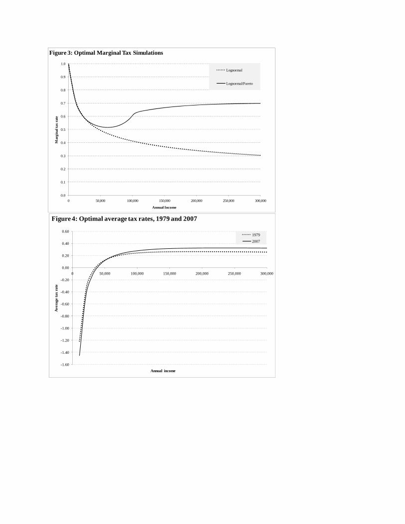
0.0

0.1

0.2

0.3

0.4

0.5

0.6

0.7

0.8

0.9

1.0

0 50,000 100,000 150,000 200,000 250,000 300,000

Mar

gina

l tax

rat

e

Annual Income

Figure 3: Optimal Marginal Tax Simulations

Lognormal

Lognormal/Pareto

-1.60

-1.40

-1.20

-1.00

-0.80

-0.60

-0.40

-0.20

0.00

0.20

0.40

0.60

0 50,000 100,000 150,000 200,000 250,000 300,000

Ave

rage

tax

rate

Annual income

1979

2007

Figure 4: Optimal average tax rates, 1979 and 2007

                          

 

  

 

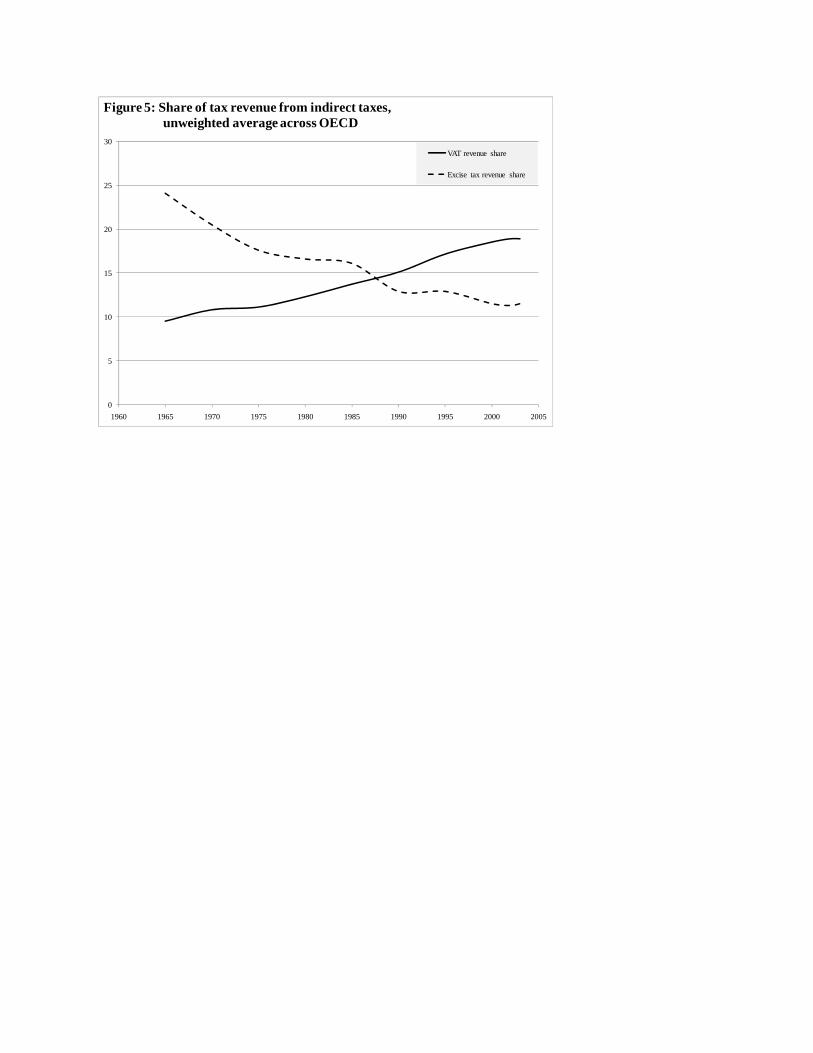
0

5

10

15

20

25

30

1960 1965 1970 1975 1980 1985 1990 1995 2000 2005

VAT revenue share

Excise tax revenue share

Figure 5: Share of tax revenue from indirect taxes,unweighted average across OECD

 

 

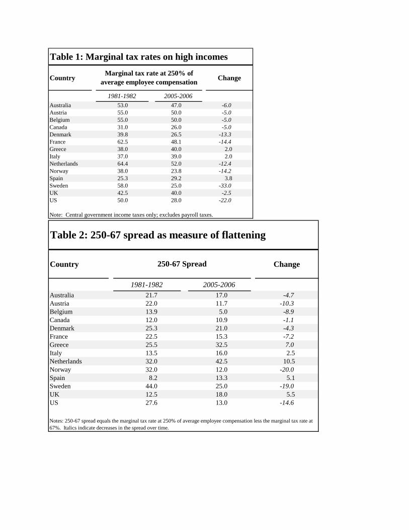
Country Change

1981-1982 2005-2006Australia 53.0 47.0 -6.0Austria 55.0 50.0 -5.0Belgium 55.0 50.0 -5.0Canada 31.0 26.0 -5.0Denmark 39.8 26.5 -13.3France 62.5 48.1 -14.4Greece 38.0 40.0 2.0Italy 37.0 39.0 2.0Netherlands 64.4 52.0 -12.4Norway 38.0 23.8 -14.2Spain 25.3 29.2 3.8Sweden 58.0 25.0 -33.0UK 42.5 40.0 -2.5US 50.0 28.0 -22.0

Table 1: Marginal tax rates on high incomes

Marginal tax rate at 250% of average employee compensation

Note: Central government income taxes only; excludes payroll taxes.   

Country Change

1981-1982 2005-2006Australia 21.7 17.0 -4.7Austria 22.0 11.7 -10.3Belgium 13.9 5.0 -8.9Canada 12.0 10.9 -1.1Denmark 25.3 21.0 -4.3France 22.5 15.3 -7.2Greece 25.5 32.5 7.0Italy 13.5 16.0 2.5Netherlands 32.0 42.5 10.5Norway 32.0 12.0 -20.0Spain 8.2 13.3 5.1Sweden 44.0 25.0 -19.0UK 12.5 18.0 5.5US 27.6 13.0 -14.6

Table 2: 250-67 spread as measure of flattening

250-67 Spread

Notes: 250-67 spread equals the marginal tax rate at 250% of average employee compensation less the marginal tax rate at 67%. Italics indicate decreases in the spread over time.  

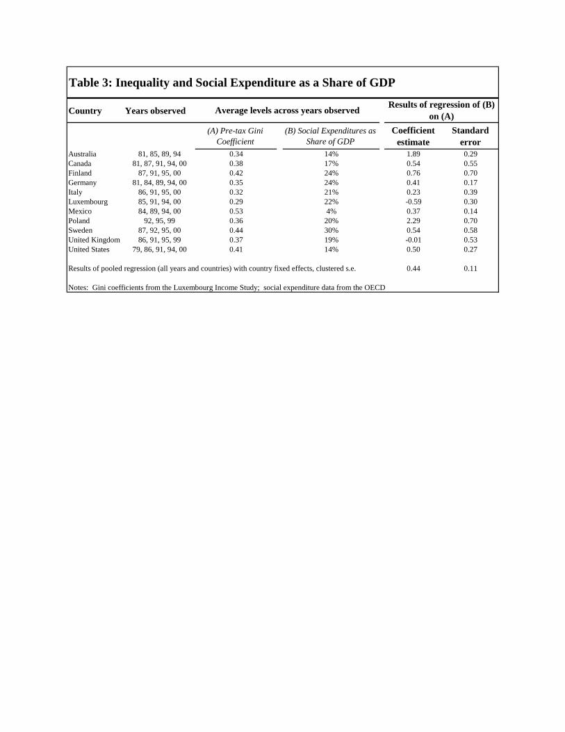
Country Years observed

(A) Pre-tax Gini Coefficient

(B) Social Expenditures as Share of GDP

Coefficient estimate

Standard error

Australia 81, 85, 89, 94 0.34 14% 1.89 0.29Canada 81, 87, 91, 94, 00 0.38 17% 0.54 0.55Finland 87, 91, 95, 00 0.42 24% 0.76 0.70Germany 81, 84, 89, 94, 00 0.35 24% 0.41 0.17Italy 86, 91, 95, 00 0.32 21% 0.23 0.39Luxembourg 85, 91, 94, 00 0.29 22% -0.59 0.30Mexico 84, 89, 94, 00 0.53 4% 0.37 0.14Poland 92, 95, 99 0.36 20% 2.29 0.70Sweden 87, 92, 95, 00 0.44 30% 0.54 0.58United Kingdom 86, 91, 95, 99 0.37 19% -0.01 0.53United States 79, 86, 91, 94, 00 0.41 14% 0.50 0.27

Results of pooled regression (all years and countries) with country fixed effects, clustered s.e. 0.44 0.11

Notes: Gini coefficients from the Luxembourg Income Study; social expenditure data from the OECD

Table 3: Inequality and Social Expenditure as a Share of GDP

Average levels across years observedResults of regression of (B)

on (A)