Optimal Sparse Matrix Dense Vector

Multiplication in the I/O-Model

Michael A. BenderDepartment of Computer Science,

Stony Brook University,Stony Brook, NY 11794-4400, USA.

bender@cs.sunysb.edu

Gerth Stølting BrodalMADALGO∗, Department of Computer Science,

Aarhus University,Aarhus, Denmark.

gerth@cs.au.dk

Rolf FagerbergDepartment of Mathematics and Computer Science,

University of Southern Denmark,Odense, Denmark.rolf@imada.sdu.dk

Riko JacobTechnische Universitat Munchen,Department of Computer Science,

Munich, Germany.jacob@in.tum.de

Elias VicariETH Zurich,

Institute of Theoretical Computer Science,8092 Zurich, Switzerland.

vicariel@inf.ethz.ch

August 23, 2010

∗Center for Massive Data Algorithmics - a Center of the Danish National Research Foun-dation

1

Abstract

We study the problem of sparse-matrix dense-vector multiplication(SpMV) in external memory. The task of SpMV is to compute y := Ax,where A is a sparse N ×N matrix and x is a vector. We express sparsityby a parameter k, and for each choice of k consider the class of matriceswhere the number of nonzero entries is kN , i.e., where the average numberof nonzero entries per column is k.

We investigate what is the external worst-case complexity, i.e., thebest possible upper bound on the number of I/Os, as a function of k, Nand the parameters M (memory size) and B (track size) of the I/O-model.We determine this complexity up to a constant factor for all meaningfulchoices of these parameters, as long as k ≤ N1−ε, where ε depends onthe problem variant. Our model of computation for the lower bound is acombination of the I/O-models of Aggarwal and Vitter, and of Hong andKung.

We study variants of the problem, differing in the memory layout of A.If A is stored in column major layout, we prove that SpMV has I/O com-

plexity Θ“

minn

kNB

maxn

1, logM/BN

maxk,M

o, kN

o”for k ≤ N1−ε and

any constant 0 < ε < 1. If the algorithm can choose the memory layout,

the I/O complexity reduces to Θ“

minn

kNB

maxn

1, logM/BN

kM

o, kN

o”for k ≤ 3

√N . In contrast, if the algorithm must be able to

handle an arbitrary layout of the matrix, the I/O complexity is

Θ“

minn

kNB

maxn

1, logM/BNM

o, kN

o”for k ≤ N/2.

In the cache oblivious setting we prove that with tall cache assumption

M ≥ B1+ε, the I/O complexity is O“

kNB

maxn

1, logM/BN

maxk,M

o”for

A in column major layout.

Categories and Subject Descriptors: F.2 [Theory of Computation]: Anal-ysis of Algorithms and Problem ComplexityGeneral Terms: Algorithms, TheoryKeywords: I/O-Model, External Memory Algorithms, Lower Bound, SparseMatrix Dense Vector Multiplication

2

1 Introduction

Sparse-matrix dense-vector multiplication (SpMV) is one of the core operationsin the computational sciences. The task of SpMV is to compute y := Ax, whereA is a sparse matrix (most of its entries are zero) and x is a vector. Applicationsabound in scientific computing, computer science, and engineering, including it-erative linear-system solvers, least-squares problems, eigenvalue problems, datamining, and web search (e.g., computing page rank). In these and other appli-cations, the same sparse matrix is used repeatedly; only the vector x changes.

From a traditional algorithmic point of view (e.g., the RAM model), theproblem is easily solved with a number of operations proportional to the num-ber of nonzero entries in the matrix, which is optimal. In contrast, empiricalstudies show that this naıve algorithm does not use the hardware efficiently;for example [18] reports that CPU-utilization is typically as low as 10% for thisalgorithm. The explanation lies in the memory system of modern computers,where access to a data item takes a few CPU cycles when the item is currentlystored in cache memory, but significantly more if the item needs to be fetchedfrom main memory, and much more if the item resides on disk. Hence, opti-mizing for the memory hierarchy is important for achieving efficiency in manycomputational tasks, including the SpMV problem.

Previous theoretical considerations The memory hierarchy of a computeris usually modeled by the I/O-model [1] (also known as the DAM-model) andthe cache-oblivious model [8]. The I/O-model is a two-level abstraction ofa memory hierarchy, modeling either cache and main memory, or main mem-ory and disk. The inner memory level has limited size M , the outer level isunbounded, and transfers between the two levels take place in tracks of size B.Computation can only take place on data residing in the inner memory level,and the cost of an algorithm is the number of track transfers, or I/Os, performedbetween the two memory levels. The cache-oblivious model is essentially theI/O-model, except that the track size B and main memory size M are unknownto the algorithm designer. More precisely, algorithms are expressed in the RAMmodel, but analyzed in the I/O-model (assuming an optimal cache replacementpolicy). The main virtue of the model is that an algorithm proven efficientin the I/O-model for all values of B and M is automatically efficient on anunknown, multilevel memory hierarchy [8]. Thus, the cache-oblivious modelenables one to reason about a two-level model while proving results about anunknown multilevel memory hierarchy.

These models were successfully used to analyze the I/O complexity of sort-ing and permuting. In the I/O-model it was shown that the optimal boundfor comparison based sorting N data items is O

(NB logM/B

NM

)I/Os and for

permuting N data items it is O(

minN, NB logM/BNM )

I/Os [1].1

1Throughout the paper log stands for the binary logarithm and logb x := max1, logb x.We also use notation ` = O (f(N, k, M, B)) with the established meaning that there exists aconstant c > 0 such that ` ≤ c · f(N, k, M, B) for all valid N, k, M , and B.

3

In the cache-oblivious model permuting and sorting can both be performedin O

(NB logM/B

NM

)I/Os, provided M ≥ B1+ε for some constant ε > 0 (the

so-called tall cache assumption) [8], and provably no algorithm can achieve theI/O bounds from the I/O-model in the cache-oblivious model [3]. Permuting isa special case of sparse matrix-vector multiplication (with sparsity parameterk = 1), namely where the matrix is a permutation matrix. There are classes ofpermutation matrices for which the complexity of the problem is known [5]. Inits classical formulation [1], the I/O-model assumes that data items are atomicrecords which can only be moved, copied, or destroyed. Hence, the I/O-modeldoes not directly allow to consider algebraic tasks, as we do here. In particular,for lower bounds a specification of the algebraic capabilities of the model isneeded. One specification was introduced in the red-blue pebble game of Hongand Kung [9] (which captures the existence of two levels of memory, but does notassume that I/O operations consist of tracks, i.e., it assumes B = 1). Another isimplicit in the lower bound proof for FFT in [1]. There are other modificationsof the I/O-model known which are geared towards computational geometryproblems [2].

Previous practical considerations In many applications where sparse ma-trices arise, these matrices have a certain well-understood structure. Exploitingsuch structure to define a good memory layout of the matrix has been donesuccessfully; examples of techniques applicable in several settings include “reg-ister blocking” and “cache blocking,” which are designed to optimize registerand cache use, respectively. See, e.g., [18, 6] for excellent surveys of the dozensof papers on this topic, and [18, 17, 10, 13, 12, 7] for sparse matrix libraries. Inthis line of work, the metric is the running time on test instances and currenthardware. This is in contrast to our considerations, where the track size Band the memory size M are the parameters and the focus is on asymptotic I/Operformance.

Problem definition and new results In this paper, we consider N×N ma-trices A and quantify their sparsity by their number of nonzero entries. Moreprecisely, a sparsity parameter k bounds the total number of nonzero entriesof A by kN , i.e., the average number of nonzero entries per column is at most k.For a given value of k, we consider algorithms that work for all matrices withat most kN nonzero entries, and we are interested in the worst-case I/O perfor-mance of such algorithms as a function of the dimension N of the matrix, thesparsity parameter k, and the parameters M and B of the I/O-model. Whenwe need to refer to the actual positions of the nonzero entries of a given matrix,we denote these the conformation of the matrix.

We assume that a sparse matrix is stored as a list of triples (i, j, x) describingthat at position (row i, column j) the value of the nonzero entry aij is x. Theorder of this list corresponds to the layout of the matrix in memory. In thispaper, we consider the following types of layouts. Column major layoutmeans that the triples are sorted lexicographically according to j (primarily)

4

Table 1: Summary of the I/O performance of the algorithms in Section 3(∗cache-oblivious).

Sect. 3.1 Naıve algorithm, row and column major O (kN)∗

Sect. 3.2 Worst case (all layouts) O(kNB logM/B

NM

)∗Sect. 3.3 Column major O

(kNB logM/B

Nmaxk,M

)∗Sect. 3.4 Best case (blocked row major) O

(kNB logM/B

NkM

)

and i (to break ties). Symmetrically, row major layout means that the triplesare sorted lexicographically according to i (primarily) and j (to break ties). Ifthe algorithm is allowed to choose any contiguous layout of the matrix, we referto this situation as the best case layout. If an arbitrary contiguous layout ispart of the problem specification, it is called worst case layout. Regarding thelayout of the input and output vectors, we most of the time assume the elementsto be stored contiguous in the order x1, x2, . . . , xN , but we also consider the casewhere the algorithm is allowed to choose a best case contiguous layout of thesevectors.

Our contributions in this paper are as follows and summarized in Table 1:

• We extend the I/O-model Aggarwal and Vitter [1] by specific algebraiccapabilities, giving a model of computation which can be seen as a com-bination of the I/O-model and the model of Hong and Kung [9].

• We give an upper bound parameterized by k on the cost for SpMV whenthe (nonzero) entries of the matrices are stored in column major layout.Specifically, the I/O cost for SpMV isO

(min

kNB logM/B

Nmaxk,M , kN

).

This bound generalizes the permuting bound, where the first term de-scribes a generalization of sorting by destination, and the second termdescribes moving each element directly to its final destination.

• We show that when the (nonzero) entries of the matrices are stored in anorder specified by the algorithm (best case layout), the I/O cost for SpMVreduces to O

(min

kNB logM/B

NkM , kN

).

• We give a lower bound parameterized by k on the cost for SpMV whenthe nonzero entries of the matrices are stored in column major layout ofΩ(

minkNB logM/B

Nmaxk,M , kN

)I/Os. This result applies for k ≤

N1−ε, for all constant 0 < ε < 1. This shows that our correspondingalgorithm is optimal up to a constant factor.

• We determine the I/O-complexity parameterized by k on the cost forSpMV when the layout of the matrix is part of the problem specifica-

5

tion (worst case layout) for k ≤ 3√N to be Θ

(min

kNB logM/B

NM , kN

)I/Os.

• We show a lower bound parameterized by k on the cost for SpMV whenthe layout of the matrix and the vectors is chosen by the algorithm: for kwith 8 ≤ k ≤ 3

√N we show that Ω

(min

kNB logM/B

NkM , kN

)I/Os are

required. This result shows that in this case the choice of the layout ofthe vector does not allow asymptotically faster algorithms.

• Finally, we show that in the cache oblivious setting with the tall cacheassumption M ≥ B1+ε, SpMV can be done withO

(kNB logM/B

Nmaxk,M

)I/Os if the matrix is stored in column major layout.

In this, the lower bounds take most of the effort. They rely upon a countingargument already used in [1] which we outline here: We define the notion of asemiring I/O-program (details in Section 2.2) that captures the I/O-data flowof an algorithm. We use this to compare the number of different programsusing ` I/O operations with the number of inputs that are possible for thedifferent tasks. From this we can conclude that some inputs (matrices) requirea certain number of I/O-operations. As a side result, our arguments show that auniformly chosen random sparse matrix will almost surely require half the I/Osclaimed by the worst-case lower bounds (see Section 9).

Road map of the paper In Section 2, we describe the computational modelsin which our lower bounds are proved. In Section 3, we present our upperbounds. The presentation of the lower bound results starts in Section 4 with alower bound for a simple data copying problem. In Section 5 we use the lowerbound for the data copying problem to derive a lower bound for SpMV for thecase of worst case layout. In Section 6 we present the lower bound for the case ofcolumn major layout, and in Section 7 we presents the lower bound for best caselayouts. We may also consider allowing the algorithm to choose the layout of theinput and output vectors. In Section 8, we show that this essentially does nothelp algorithms already allowed to choose the layout of the matrix. Section 9discusses additional variations on the results, and possible future work.

2 Models of Computation

Our aim is to analyze the I/O cost of SpMV. As I/Os are generated by movementof data, we effectively are studying what data flows are necessary for performingthe computations involved in SpMV, and how these data flows interact with thememory hierarchy. The final result, i.e., the entries of the output vector, is aset of algebraic expressions, so we need a model specifying both the memoryhierarchy and the algebraic capabilities of our machine.

In this section, we define two such models, one to formulate algorithms, andanother one to prove lower bounds. By I/O-model we mean in this paper

6

the model used to formulate algorithms as explained in Section 2.1 and usedin Section 3. In contrast, we prove the lower bounds for so called semiringI/O-programs, as explained in detail in Section 2.2. The relation between thetwo models is explained in Section 2.3, where we argue that a lower bound forsemiring I/O-programs also applies to the I/O-model used to formulate algo-rithms.

Both models combine ideas from the I/O-model of Aggarwal and Vitter [1]previously used to analyze the problem of permuting (a special case of SpMV),with the algebraic capabilities used by Hong and Kung [9] under the name “in-dependent evaluation of multivariate expressions” for analyzing matrix-matrixmultiplication. They are based on the notion of a commutative semiring S.This is a set of elements with addition (x+ y) and multiplication (x× y or xy)operations. These operations are associative and commutative, and distributive.There is a neutral element 0 for addition, a neutral element 1 for multiplication,and multiplication with 0 yields 0. In contrast to a field, there are no inverseelements guaranteed, neither for addition nor for multiplication. One well inves-tigated example of such a semiring (actually having multiplicative inverses) isthe max-plus algebra (tropical algebra), in which matrix multiplication can beused, for example, to compute shortest paths with negative edge length. Otherwell known semirings are the natural, rational, real or complex numbers withthe usual addition and multiplication operations. In the following, we denotethe elements of the semiring as numbers.

2.1 The I/O-model

The I/O-model is the natural extension of the I/O-model of Aggarwal andVitter [1] to the situation of matrix-vector multiplication. It models main mem-ory to consist of M data atoms, and disk tracks of B data atoms. We countthe number of I/O-operations that transfer such a track between main memoryand the disk. Here, data atoms are either integers (e.g., used to specify rowsor columns of the matrix and positions in a layout) or they are elements froma semiring. In particular, elements of the semiring cannot be compared witheach other. All computation operations require that the used data items arecurrently stored in main memory.

2.2 Semiring I/O-programs

In contrast to the algorithmic model, for the lower bound we consider a non-uniform setting. This means that an algorithm is given by a family of semiringI/O-programs, one program for each conformation (including N and k) of thematrix, irrespective of the underlying semiring and numbers. The layout ofthe matrix can be implied by the conformation (e.g., column major layout),part of the conformation (worst-case layout), or part of the program (best-case layout). Such a semiring I/O-program is a finite sequence of operationsexecuted sequentially (without branches or loops) on the following abstract ma-chine: there is a disk D of infinite size, organized in tracks of B numbers each,

7

and a main memory containing M numbers, with all numbers belonging toa commutative semiring S. A configuration of the model is a vector of Mnumbers M = (m1, . . . ,mM ) ∈ SM , and an infinite sequence D of track vec-tors ti ∈ SB . Initially, all numbers not part of the input have the value 0. Astep of a computation leads to a new configuration according to the followingallowed operations:

• Computation on semiring numbers in main memory: algebraic opera-tions mi := mj + mk, mi := mj ×mk, setting mi := 0, setting mi := 1,and assigning mi := mj .

• Read: move an arbitrary track of the disk into the first B cells of memory,(m1, . . . ,mB) := ti; ti := 0. The cells are required to be empty prior tothe read ((m1, . . . ,mB) = 0).

• Write: move the first B cells of memory to an arbitrary track, ti :=(m1, . . . ,mB); (m1, . . . ,mB) := 0. The track is required to be emptyprior to the write (ti = 0).

Read and write operations are collectively called I/O-operations. We say thatan algorithm for SpMV runs in (worst-case) `(k,N) I/Os if for all N , all k, andall conformations for N×N matrices with kN nonzero coefficients, the programchosen by the algorithm performs at most `(k,N) I/Os.

Intermediate results During the execution of a program, the disk and themain memory contain numbers, which are either part of the input (i.e., matrixand input vector entries), are one of the two neutral elements 0 and 1 of thesemiring, or are the result of a series of semiring operations. We call the num-bers appearing during the run of a program for intermediate results. Oneintermediate result p is a predecessor of another p′ if it is an input to theaddition or multiplication leading to p′, and is said to be used for calculatingp′ if p is related to p′ through the closure of the predecessor relation. By thecommutativity of addition and multiplication, every intermediate result may bewritten in the form of a polynomial, with integer coefficients, in the xj ’s of theinput vector and the nonzero aij ’s of the matrix—that is, as a sum of monomialswhere each monomial is a product of xj ’s and aij ’s, each raised to some power,and one element from 1, 1+1, 1+1+1, . . . . We call this the canonical formof an intermediate result.

The degree of a canonical form is the largest sum of powers that occur in oneof the monomials. If two canonical forms f and g are multiplied or added, thenthe set of variables in the resulting canonical form is the union of the variablesof f and g. For multiplication, the degree is equal to the sum of the degrees.For addition, the number of monomials and the degree cannot decrease.

Note that the canonical forms themselves form a semiring, called the freecommutative semiring over the input numbers. Because of this it is impossiblethat two different canonical forms stand for the same element in all possiblesemirings. Hence, the final results yi of SpMV are the unique canonical forms

8

yi =∑j∈Ri 1× aij × xj of degree at most two. Here Ri is the set of columns in

which row i has nonzero entries, which depends only on the conformation of thematrix. By a similar reasoning, as detailed in Lemma 2.1 below, we may assumethat each intermediate value is a “subset” of a final result, i.e., it has one ofthe following forms: xj , aij , aijxj , or si =

∑j∈S aijxj , where 1 ≤ i, j ≤ N ,

S ⊆ Ri ⊆ 1, . . . , N. These forms are called, respectively, input variable,coefficient, elementary product, and partial sum. We call i the row of thepartial sum. If S = Ri, we simply denote the partial sum a result. Collectively,we call these forms canonical partial results. Every canonical partial resultbelongs in a natural way to either a column (j for xj) or a row (i for the rest ofthe canonical partial results).

Lemma 2.1 If there is a program which multiplies a given matrix A with anyvector in the semiring I/O-model using ` I/Os, then there is also a programperforming the same computation using ` I/Os, but computing only canonicalpartial results and never having two canonical partial sums of the same row inmemory immediately before an I/O is performed.

Proof. Assume that the canonical form f represents an intermediate result.If f contains a monomial of degree one (i.e., single variables or coefficients), itneeds to be multiplied with a non-constant canonical form before it can becomea final result. Hence, if it contains two different monomials of degree one, therewill be products of two variables or two coefficients, or a product of a variablewith a coefficient of the wrong column. Such an f cannot be used for a finalresult. The following four properties of f will be inherited by anything derivedfrom f and hence prevent f from being used for any final result.

1. f has degree of three or more,

2. f has a poly-coefficient of 1 + 1 or larger,

3. f contains matrix entries from different rows,

4. f contains the product of two vector variables or two matrix entries.

From this we can conclude that a useful intermediate result f must be a canon-ical partial result (by case analysis of the degree of f).

Clearly, intermediate results that are computed but are not used for a finalresult may as well not be computed. Similarly, the 0-canonical form is equivalentto the constant 0 and any occurrence of it as intermediate result can be replacedby the constant 0.

Finally, observe that partial sums can only be used in summations thatderive new partial sums or final results. Hence, if two partial sums pi and qithat both are used to eventually derive yi are simultaneously in memory, theycan be replaced by p′i = pi + qi and the constant q′i = 0 (not a partial sum)without changing the final result. ut

9

2.3 Connection between algorithmic and lower bound model

The two introduced models only make sense if the complexities in the two modelsare essentially the same:

Lemma 2.2 Every algorithm A for SpMV in the I/O-model with I/O-complexity`(k,N) gives rise to a family of semiring I/O-programs using at most `(k,N)I/Os.

Proof. Fix k, N , a matrix conformation and its layout. Because the branchesand loops of the algorithm do not depend on the semiring values, we can sym-bolically execute the algorithm A and finally ignore all computations on non-semiring variables. This leads to a family of semiring I/O-programs that use nomore I/Os than A. Here the layout of the matrix can either be fixed, part ofthe input or part of the program, precisely in the same way as for A. ut

It follows that lower bounds for semiring I/O-programs translate into lowerbounds for algorithms in the I/O-model. For the case of worst-case layout, itis noteworthy that the algorithms we propose in Section 3 do not need to knowthe layout in advance.

3 Algorithms

In this section we describe several algorithms for solving SpMV. All algorithmscompute the necessary elementary products aijxj (in some order) and thencompute the sums yi =

∑Nj=1 aijxj (in some order). We describe different algo-

rithms for each of the possible layouts: row major, column major, worst case,and best case. The bounds achieved are summarized in Table 1. Through-out this section we assume that x is given in an array such that we can scanthe sequence x1, x2, . . . , xN using O (N/B) I/Os. We assume 1 ≤ k ≤ N andM ≥ 3B.

3.1 Naıve Algorithm

We first describe how the layout of a matrix influences the I/O performanceif we simply perform a sequential scan over all triples (i, j, aij) and repeatedlyupdate yi := yi + aijxj to solve the SpMV problem. In internal memory thisapproach yields an optimal O (kN) time algorithm, but for both row major andcolumn major layouts we get poor I/O performance—but for different reasons.

Row major layout In row major layout we finish computing yi before ad-vancing to compute yi+1. The nonzero entries in a row i of A are in the worstcase sparsely distributed such that each xj accessed while computing yi is in anew track, in the worst case causing an I/O to fetch each xj . While scanningall triples in total costs O (kN/B) I/Os and updating y costs O (N/B) I/Os,the bottleneck becomes accessing x, causing in the worst case a total of O (kN)I/Os.

10

Column major layout The algorithm performs a single sequential scan of thelist of the kN triples for the nonzero entries of A while simultaneously perform-ing a single scan of all entries in x, i.e. we compute all products yijxj involvingxj before advancing to xj+1. The cost of accessing A and x is O (kN/B) I/Os.While updating yi := yi + aijxj we potentially skip many entries of y betweenconsecutive updates, such that each of the kN updates to y in the worst casecauses one read and one write I/O. It follows that in the worst-case the totalnumber of I/Os is O (kN).

Note that while for row major layout the I/O bottleneck was to access x itfor column major layout are the updates to y that become the bottleneck.

3.2 Worst Case Layout

A generic algorithm to multiply A with x, without any assumption on the layoutof the nonzero entries of A, is the following.

1. Sort all triples (i, j, aij) by j.

2. Scan the list of all triples (i, j, aij) (in increasing j order) while simulta-neous scanning x and generating all triples (i, j, aijxj).

3. Sort all triples (i, j, aijxj) by i.

4. Scan the list of all triples (i, j, aij) (in increasing i order) while addingconsecutive triples generating the sums yi =

∑Nj=1 aijxj .

Steps 1 and 3 sort kN elements using O(kNB logM/B

kNM

)I/Os [1], while

Steps 2 and 4 scanO (kN) elements usingO (kN/B) I/Os. In totalO(kNB logM/B

kNM

)I/Os are used.

The logarithm in the above bound can be reduced by partitioning the kNcoefficients into k groups each of size N (using an arbitrary partitioning). Byusing the above algorithm for each of the k groups we use O

(NB logM/B

NM

)I/Os per group. The results are k vectors of size N with partial results. Byadding the k vectors using O (kN/B) I/Os we compute the final output vector y.In total we use O

(kNB logM/B

NM

)I/Os.

3.3 Column Major Layout

If A is given in column major layout the algorithm in Section 3.2 can be im-proved. Step 1 can be omitted since the triples are already sorted by increas-ing j. Step 2 remains unchanged. After Step 2 we have for each column j alltriples (i, j, aijxj) sorted by i. We split the columns into at most 2k groups,each group consisting of at most N/k columns and at most N triples. For eachgroup we have at most N/k sequences of triples sorted by i. For each group we

11

compute the merged sequence of triples using an I/O-optimal merger. Since t se-quences with a total of s elements can be merged usingO

(sB logM/B mint, sM

)I/Os [4], the merging in total for all groups requires O

(kNB logM/B

Nmaxk,M

)I/Os. By scanning the output of each group we can compute a vector of N par-tial results for each group using a total of O (kN/B) I/Os, since groups aresorted by i. Finally we add the k vectors using O (kN/B) I/Os. The total I/Ocost becomes O

(kNB logM/B

Nmaxk,M

).

3.4 Best Case Layout

By adopting a different input layout to the algorithm in Section 3.3 we canachieve a further speedup. Assume we store the coefficients of A in slabs ofM − 2B consecutive full columns, where each such slab is stored in row majorlayout. This layout allows a sequentially scan of the triples (i, j, aij) to generatethe triples (i, j, aijxj) in total O (kN/B) I/Os, by having the window of theM−2B elements from x in memory corresponding to the columns of the currentslab. The resulting sequence of triples consists of N/(M − 2B) subsequencessorted by i. As in Section 3.3 we split the generated triples into 2k groups, butnow each group only consists of N

k(M−2B) = O(NkM

)sorted sequences to merge.

The rest of the algorithm and analysis remains unchanged. The total I/O costbecomes O

(kNB logM/B

NkM

).

3.5 Cache Oblivious Algorithms

The algorithms in Section 3.2 and Section 3.3 can be implemented cache obliv-iously (under the tall cache assumption M ≥ B1+ε, as is needed for optimalsorting in this model [3]), by using a cache-oblivious sorting algorithm [8] forsorting steps and using the Run-optimal cache-oblivious adaptive sorting algo-rithm of [4, Section 5] for merging steps. Under the tall cache assumption theasymptotic I/O complexities remain unchanged.

4 Lower Bound for a Copying Problem

Central to our lower bound arguments for the SpMV problem will be the analysisof a copying problem which distributes N input values into H specified outputpositions in memory. In this section, we consider that problem on its own, ina way which will allow us to reuse the central part of the analysis in differentsettings in later sections. Specifically, Lemma 4.2 will be referenced repeatedly(Section 5 can reuse a bit more of the analysis, and therefore references laterlemmas of Section 4).

In the N-H copy problem, an instance is specified by an index ij ∈ [N ]for each j ∈ [H], where [N ] = 1, . . . , N, and the task is to transform an inputvector (x1, . . . , xN ) of N variables into the vector (xi1 , xi2 , xi3 , . . . , xiH ). In this

12

section, we show a lower bound on `(H,N), the worst case number of I/Osnecessary to perform any such task, seen as a function of H and N . We for thisproblem assume the I/O-model of Aggarwal and Vitter [1], i.e., the entries xiof the input vector are atomic and can only be moved, copied, or deleted.

The remaining of this section is devoted to prove the following lower boundtheorem:

Theorem 4.1 For every N and H where N/B ≤ H ≤ N2, there exists anN -H copy problem (i1, . . . , iH) ∈ [N ]H that requires at least

minH

6,H

4BlogM

B

N

M

I/Os in the I/O-model of Aggarwal and Vitter [1].

In our analysis, we will during the execution of the algorithm consider thecontents of the main memory, and of each track on disk, as sets. That is, insideeach of these, we will disregard order and multiplicities of elements. This viewallows us to analyze tightly the development in combinatorial possibilities asthe number of I/Os grows.

We call the values of these sets the state at a given point in time, and thesequence of states we call the trace of the program. For a state, the contentof the main memory is described by a subset M ⊆ [N ], |M| ≤ M (the indicesof the variables currently in memory). Similarly, the tracks of the disk aredescribed by a list of subsets Ti ⊆ [N ], |Ti| ≤ B (for i ≥ 1).

Note that between I/Os, the contents of main memory and of each track ondisk do not change seen as sets, if the program only copies and moves elements.For the N -H copy problem, any element created which is not used for the outputmay as well not be created. If there is an input element which does not appearin the output, we may as well assume it is deleted immediately when it entersmain memory the first time (which gives rise to no combinatorial choices in theanalysis). Hence, we can during the analysis assume deletions do not take place.

Lemma 4.2 Consider a family of programs in the I/O-model starting from theunique (set-based) state 1, . . . , B, B + 1, . . . , 2B, . . . , . . . , N and using atmost ` I/Os, assuming ` ≥ (N +H)/B and M ≥ 4B. The number of different(set-based) traces, and hence output (set-based) states, is at most((

4MB

)B4`

)`.

Proof. We assume that the program complies with the following rules: Theprogram executes precisely ` I/Os (if fewer I/Os are executed we pad the pro-gram with repeatedly writing and reading an empty track). Tracks used forintermediate results are numbered consecutively and hence require an addressspace of at most ` positions, such that together with the at most (N + H)/BI/Os to read input and write output, we get an address space of at most

13

(N +H)/B + ` ≤ 2` tracks. Any correct program can easily be transformed tocomply with the above rules without increasing the number of I/Os.

We can now bound the number of traces (equivalently, number of final states)that can be created with ` I/Os, by bounding the number of choices for gener-ating a new state when performing an I/O.

For a write operation, there is the choice of the up to B elements out ofM when creating the contents of the track. There is a difference in resultingstate if an element moved out of main memory by a write is the last copy inmain memory, or if it is not—in the former case, the content of main memory,seen as a set value, changes, in the latter case, it does not. In the analysis, wemove this combinatorial choice to the reads (since the combinatorial choices ofwrites already dominate in the argument), and we do this by never changingthe set value of the main memory when performing a write, but instead leavethe elements of the former case as dead elements of the set. To avoid the setsize growing above M , reads now must remove enough such dead elements tomake room for the up to B elements entering main memory. Because in theactual program there is room for the elements entering main memory, there arein the analysis always enough dead elements for such a removal to be feasible.Thus, in our analysis reads also have a choice of up to B elements out of Mwhen choosing which dead elements to remove.

For writes, the number of elements written is not necessarily B, since weare considering set-based traces. Rather, a write may write out sets of sizes1, 2, . . . , B. Hence, the number of different sets which a write can choose is∑Bi=1

(Mi

). From the standard identity

∑ni=0

(ri

)(sn−i)

=(r+sn

)it follows that∑B

i=0

(Mi

)≤∑Bi=0

(Mi

)(BB−i)

=(M+BB

). With M ≥ 4B, implying M + B ≤

5M/4, and e5M/4 < 4M we get by(xy

)≤ (xe/y)y the bound

(M+BB

)≤(

4MB

)B.

For each I/O, there is also the choice of which of the at most 2` tracks ondisk it pertains to, and there is a factor of 2 to choose between read and writeoperations. ut

The above finishes our analysis of algorithms for the N -H copy problem interms of set-based traces. To account for the actual ordering and multiplicities ofelements of the output when the algorithm stops, we must add a final step in theanalysis where for each non-empty track (main memory must be empty by thedefinition of the output), a multiset is created from its set-based representation,to give the actual output of the algorithm. Multiplying with the combinatorialpossibilities for that step gives a bound on the total number of different outputswhich can be generated by ` I/Os. This number can then be compared to thenumber of different outputs the algorithm is required to be able to create. Wedo this in the following lemma.

Lemma 4.3 Assume there is a family of programs in the I/O-model computingall copying tasks using N variables and producing H outputs with ` = `(H,N)I/Os for memory size M and track size B. Then, for H ≥ N/B and M ≥ 4B

14

it must hold that

NH ≤

((4MB

)B4`

)`·BH .

Proof. During execution, we consider the contents of the main memory, andof each track on disk, as sets, and we now have to count the number of ways inwhich a set-based state describing the tracks output can be interpreted as a listof copies. Given a specific subset of [N ] residing on an output track, a variablein the final (ordered, multiset) version of the track can be expressed by the rank(a number in [B]) of the index of the variable within the subset of the track.Hence, one (set-based) trace can solve at most BH different copying tasks whenadding order and multiplicity in the end. Because there are NH copying tasks,the lemma follows from Lemma 4.2, provided ` ≥ (N +H)/B. Since H ≥ N/Bthere exists an N -H copy problem that outputs H/B blocks all different froman input block, and all N/B input blocks contain at least one element that ispart of the output, i.e., we have ` ≥ (N +H)/B. ut

To finish the proof of Theorem 4.1, we need to solve the equation of Lemma 4.3for `. We do this in the following lemma. Note that H ≥ N/B implies` ≥ (N+H)/B, as shown in the proof of Lemma 4.3, so the assumption ` ≥ H/Bbelow is justified.

Comparing to Lemma 4.3, one notes that the assumption (1) of the lemmais slightly weakened. This is done in order to match conditions in Section 5,such that we there can refer directly to Lemma 4.4.

Lemma 4.4 Assume M ≥ 4B, H ≤ N2, and ` ≥ H/B. Then(N

2

)H≤

((4MB

)B4`

)`·BH (1)

implies

` ≥ minH

4BlogM/B

N

M,H

6

.

Proof. For B ≤ 6 the bound ` ≥ H/B justifies the theorem, hence we assumeB ≥ 6. For N ≤ 210 the lemma holds trivially: Because of B ≥ 6 we haveM ≥ 24 and N/M < 26. Using M/B ≥ 4 we get logM/B

NM < 3, and hence

again the bound ` ≥ H/B justifies the theorem. Therefore, we assume N ≥ 210.If ` > H/6, the lemma holds trivially. Hence, in the following we assume` ≤ H/6, implying 4` ≤ H.

Taking logs on the main assumption (1), we get

H logN

2≤ `

(logH +B log

4MB

)+H logB .

which rewrites as

` ≥ Hlog N

2B

logH +B log 4MB

.

15

Now, we distinguish by the leading term of the denominator: If logH <B log 4M

B , we get (using log MB ≥ 2 and 2B ≤M)

` ≥ Hlog N

2B

2B(2 + log M

B

) ≥ H

4BlogM

B

N

M.

If logH ≥ B log 4MB , we use log 4M

B ≥ log 16 = 4, which leads (using H ≤N2) to B ≤ logH

log 4MB

≤ 24 logN ≤ 1

23√N for N ≥ 210. We conclude with

` ≥ Hlog(

N

2· 12 ·3√N

)2 log(N2)

= H23 logN4 logN

=H

6.

ut

5 Lower Bound for Worst-Case Layout

In this section, we give a lower bound for the SpMV problem with worst caselayout of the matrix. We consider the special case where the input vector is theall ones vector (xi = 1), i.e., we consider programs computing the row-sums ofthe matrix.

The idea of the proof is to trace backwards in time the computation of eachof the N output results si =

∑j∈Ri aij to the kN coefficients aij of the matrix

(recall that Ri is the set of column indexes of the nonzero entries of row i ofthe matrix). We will show how to interpret this time-reversed execution of asemiring I/O-program for computing row-sums as solving an instance of theN -H copy problem. This will allow us to reuse the analysis of Section 4.

To trace the program execution backwards in time, we annotate each resultsi by its row index i, and propagate these annotations backwards in time toother values appearing during the execution of the program. By Lemma 2.1and the discussion preceding it, we may assume that all values appearing areeither 0, 1, coefficients, or partial sums. We may also assume that additionsby 0 and multiplication by 1 do not take place, as such operations can beomitted without changing the output. By a case analysis of possible value typesand the operations allowed in the model (and the uniqueness of the canonicalform of a value, cf. text preceding Lemma 2.1), one sees that a partial summt =

∑j∈S aijxj with |S| ≥ 2 can only arise as the result of either the addition

mt :=∑j∈S1

aijxj +∑j∈S2

aijxj , where S1, S2 is a nontrivial partitioning of S(S1 ∪ S2 = S, S1 ∩ S2 = ∅, |S1|, |S2| ≥ 1), or the assignment mt := ms, wherems =

∑j∈S aij . In the former case, we propagate the annotation i backwards

in time to both operands of the addition. In the latter case, we propagate theannotation i backwards in time to ms. Similarly, we propagate the annotationof an elementary product aijxj back to aij at the multiplication creating thiselementary product. For read and write operations, note that these are timereverses of each other, due to the definitions of reads and writes in our model

16

(which are symmetrical, and involve moving rather than copying). For theseoperations, annotations just follow the values moved.

By induction on the number of time steps backwards in time, it follows thatat all times, all entries aij are annotated exactly once (by their row index i) if theannotation of a partial sum

∑j∈S aijxj is seen as pertaining to all coefficients aij

appearing in the sum.Given a vector (x1, . . . , xN ) of N variables, we may change the annotation

to use the variable xi instead of the integer i. This annotation, when viewedbackwards in time, defines a program for copying a vector (x1, . . . , xN ) of Nvariables into kN positions in memory, with xi being copied to the positionson disk where the nonzero coefficients of row i of the matrix reside in the givenlayout of the matrix. In other words, it is a program solving an instance of theN -H copy problem for H = kN , with the output vector (xi1 , xi2 , xi3 , . . . , xiH )specified by the matrix and its layout. It works in the I/O-model of Aggarwaland Vitter [1], and uses copying (the time reverse of addition of two partialsums), movement (the time reverse of assignment), and reads and writes (thetime reverses of each other). The number of I/Os performed is the same as theoriginal program for computing row-sums.

However, not all of the NkN instances of the N -H copy problem withH = kN can be specified by a matrix in this way, since no row has morethan N nonzero entries. More precisely, the possible instances are exactly thosewhere the output vector (xi1 , xi2 , xi3 , . . . , xikN ) has no input variable xi appear-ing more than N times. We claim that for k ≤ N/2, the number of such outputvectors is at least (N/2)kN : Construct the vector by choosing xij for increas-ing j. At some point, a given variable xi may no longer be available because ithas been used N times already. However, if this is true for more than N/2 of theN variables, more than N2/2 entries in the vector have been chosen, which is acontradiction to the assumption k ≤ N/2. Hence, at each of the kN positionsof the input vector, we have at least N/2 choices.

Therefore, by adjusting the last line of the proof of Lemma 4.3, we arrive atthe following variant of that lemma.

Lemma 5.1 Assume there is a family of semiring I/O-programs, one for eachkN -dense N × N matrix and each layout of it, computing the matrix vectorproduct. Assume all programs use ` = `(H,N) I/Os. Then, for M ≥ 4B and1 ≤ k ≤ N/2 it holds that(

N

2

)kN≤

((4MB

)B4`

)`·BkN .

Using Lemma 4.4, we get the following theorem.

Theorem 5.2 Let ` = `(k,N) be an upper bound on the number of I/O-operations necessary to solve the SpMV problem with worst case layout in thesemiring I/O-model. Then, for M ≥ 4B and 1 ≤ k ≤ N/2 it holds that

` ≥ minkN

4BlogM/B

N

M,kN

6

.

17

6 Lower Bound for Column Major Layout

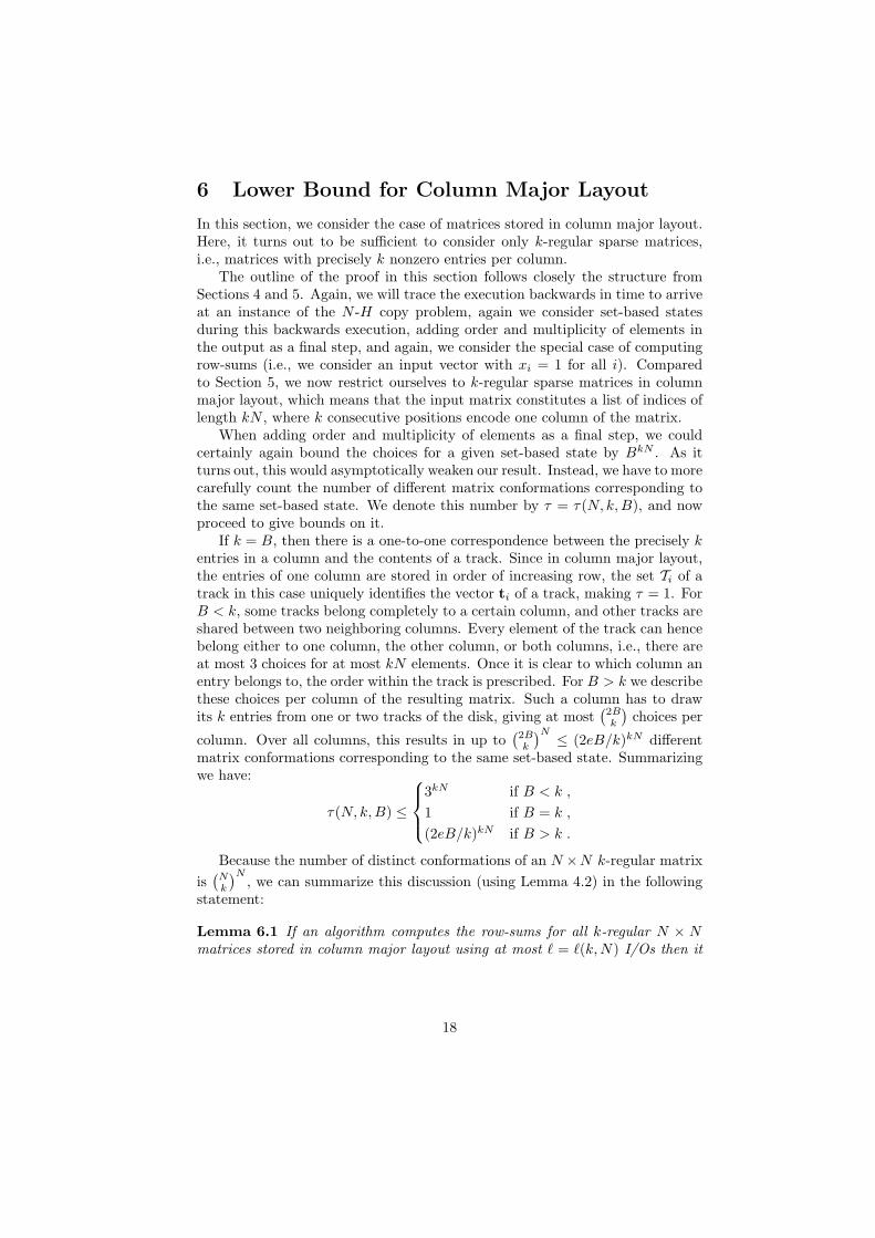
In this section, we consider the case of matrices stored in column major layout.Here, it turns out to be sufficient to consider only k-regular sparse matrices,i.e., matrices with precisely k nonzero entries per column.

The outline of the proof in this section follows closely the structure fromSections 4 and 5. Again, we will trace the execution backwards in time to arriveat an instance of the N -H copy problem, again we consider set-based statesduring this backwards execution, adding order and multiplicity of elements inthe output as a final step, and again, we consider the special case of computingrow-sums (i.e., we consider an input vector with xi = 1 for all i). Comparedto Section 5, we now restrict ourselves to k-regular sparse matrices in columnmajor layout, which means that the input matrix constitutes a list of indices oflength kN , where k consecutive positions encode one column of the matrix.

When adding order and multiplicity of elements as a final step, we couldcertainly again bound the choices for a given set-based state by BkN . As itturns out, this would asymptotically weaken our result. Instead, we have to morecarefully count the number of different matrix conformations corresponding tothe same set-based state. We denote this number by τ = τ(N, k,B), and nowproceed to give bounds on it.

If k = B, then there is a one-to-one correspondence between the precisely kentries in a column and the contents of a track. Since in column major layout,the entries of one column are stored in order of increasing row, the set Ti of atrack in this case uniquely identifies the vector ti of a track, making τ = 1. ForB < k, some tracks belong completely to a certain column, and other tracks areshared between two neighboring columns. Every element of the track can hencebelong either to one column, the other column, or both columns, i.e., there areat most 3 choices for at most kN elements. Once it is clear to which column anentry belongs to, the order within the track is prescribed. For B > k we describethese choices per column of the resulting matrix. Such a column has to drawits k entries from one or two tracks of the disk, giving at most

(2Bk

)choices per

column. Over all columns, this results in up to(2Bk

)N ≤ (2eB/k)kN differentmatrix conformations corresponding to the same set-based state. Summarizingwe have:

τ(N, k,B) ≤

3kN if B < k ,

1 if B = k ,

(2eB/k)kN if B > k .

Because the number of distinct conformations of an N ×N k-regular matrixis(Nk

)N, we can summarize this discussion (using Lemma 4.2) in the following

statement:

Lemma 6.1 If an algorithm computes the row-sums for all k-regular N × Nmatrices stored in column major layout using at most ` = `(k,N) I/Os then it

18

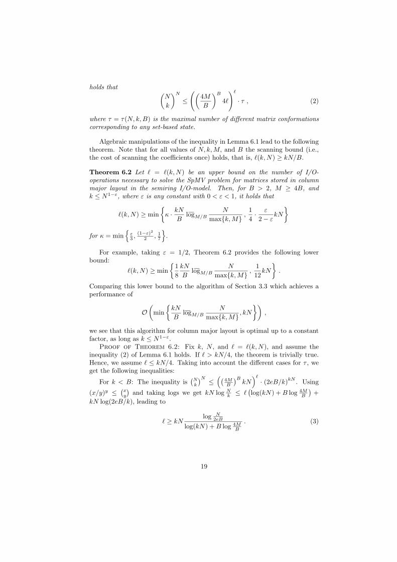
holds that (N

k

)N≤

((4MB

)B4`

)`· τ , (2)

where τ = τ(N, k,B) is the maximal number of different matrix conformationscorresponding to any set-based state.

Algebraic manipulations of the inequality in Lemma 6.1 lead to the followingtheorem. Note that for all values of N, k,M, and B the scanning bound (i.e.,the cost of scanning the coefficients once) holds, that is, `(k,N) ≥ kN/B.

Theorem 6.2 Let ` = `(k,N) be an upper bound on the number of I/O-operations necessary to solve the SpMV problem for matrices stored in columnmajor layout in the semiring I/O-model. Then, for B > 2, M ≥ 4B, andk ≤ N1−ε, where ε is any constant with 0 < ε < 1, it holds that

`(k,N) ≥ minκ · kN

BlogM/B

N

maxk,M,

14· ε

2− εkN

for κ = min

ε3 ,

(1−ε)22 , 1

7

.

For example, taking ε = 1/2, Theorem 6.2 provides the following lowerbound:

`(k,N) ≥ min

18kN

BlogM/B

N

maxk,M,

112kN

.

Comparing this lower bound to the algorithm of Section 3.3 which achieves aperformance of

O(

minkN

BlogM/B

N

maxk,M, kN

),

we see that this algorithm for column major layout is optimal up to a constantfactor, as long as k ≤ N1−ε.

Proof of Theorem 6.2: Fix k, N , and ` = `(k,N), and assume theinequality (2) of Lemma 6.1 holds. If ` > kN/4, the theorem is trivially true.Hence, we assume ` ≤ kN/4. Taking into account the different cases for τ , weget the following inequalities:

For k < B: The inequality is(Nk

)N ≤ (( 4MB

)BkN)`· (2eB/k)kN . Using

(x/y)y ≤(xy

)and taking logs we get kN log N

k ≤ `(log(kN) +B log 4M

B

)+

kN log(2eB/k), leading to

` ≥ kNlog N

2eB

log(kN) +B log 4MB

. (3)

19

For k ≥ B: From(Nk

)N ≤ ((4MB

)BkN)`· 3kN by taking logs we get

kN log Nk ≤ `

(log(kN) +B log 4M

B

)+ kN log 3, i.e.,

` ≥ kNlog N

3k

log(kN) +B log 4MB

. (4)

Combining (3) and (4) we get

` ≥ kNlog N

max3k,2eB

log(kN) +B log 4MB

. (5)

For small N ≤ max22/(1−ε)2 , 161/ε, 91/ε, 210, 16B, this bound is perhapsweak, but the statement of the theorem is justified by the scanning bound` ≥ kN/B for accessing all kN entries of the matrix: If N ≤ 22/(1−ε)2 , thenlogM/B N ≤ 2/(1 − ε)2. If N ≤ 161/ε then logM/B N ≤ 2/ε. If N ≤ 16B thenlogM/B

NM ≤ −1 + log2 16 = 3. Similarly, N ≤ 210 implies logM/B

NM ≤ 7.

Otherwise, for large N , distinguish between the dominating term in thedenominator. Fix an 0 < ε < 1 and assume that k ≤ N1−ε; if log(kN) ≥B log 4M

B we get

` ≥ kNlog N

max3k,2eB

2 log(kN)

Now, Lemma A.3 gives B ≤ 3N1−ε/2e, and using k ≤ N1−ε, N > 32/ε we get

` ≥ kN log N

3N1−ε2 log(kN) ≥ kN

ε logN−log 32(2−ε) logN ≥ kN

ε/2 logN2(2−ε) logN ≥

εkN8−4ε .

Otherwise (log(kN) < B log 4MB )), by using log M

B ≥ 2 and e < 4 (in eB ≤

M), we get ` ≥ kNlog N

max3k,2eB

2B log 4MB

≥ kN2B ·

log N3 maxk,M

log MB +2

≥ kN2B ·

− 85+log N

maxk,M

2 log MB

.

Now, we use N ≥ 16B, which, together with N/k ≥ Nε ≥ 16 for N ≥ 161/ε,implies log N

maxk,B > 4. Hence,

` ≥ kN

2B·

35 log N

maxk,M

2 log MB

≥ kN

7B· logM

B

N

maxk,M.

The log in the statement of the theorem is justified by the scanning bound. ut

7 Lower Bound for Best Case Layout

In this section, we consider algorithms that are free to choose the layout of thematrix on the disk; we refer to this case as the best case matrix layout. In thissetting, computing row-sums can be done by a single scan if the matrix is storedin row major layout. Hence, the input vector needs to become part of the lowerbound argument, and we will now trace both the movements of input variablesand the movements of partial sums while the algorithm is executing.

20

Intuitively, each input variable xj needs to disperse to meet and join a partialresult

∑j∈S aijxj for all i with aij 6= 0, while the partial results created during

the run of the program need to be combined to the final output results. The firstis a copying process in the forward direction, while the latter may be seen as acopying process in the backwards direction (similar to the analysis in Section 5and 6). Note that once the algorithm has chosen how to copy the input variables,and at what points in time they should join partial results, the access to therelevant matrix coefficient aij (for creating the elementary product aijxj to beadded to a partial result, or form one itself) is basically for free: each matrixcoefficient aij is needed exactly once, and for best case layout, the algorithmcan choose to lay out the matrix in access order, making the entire access tomatrix coefficients become a single scan.

Set up To formalize the intuition above, we use an accounting scheme whichencapsulates the internal operations between each pair of consecutive I/Os andabstracts away the specific multiplications and additions, while capturing thecreation and movement of partial results and variables. We call the semiringI/O-model extended with this accounting scheme the separated model. Wenow describe the accounting scheme.

In between two I/Os, we define the input variable memory MV ⊆ [N ],|MV | ≤ M to be the set of indices of input variables contained in memoryright after the preceding I/O, before the internal computation between the I/Osstarts, and we define the result memoryMR ⊆ [N ], |MR| ≤M to be the set ofrow indices of the matrix for which some partial sum or coefficient is in mem-ory after the internal computation has taken place, right before the succeedingI/O. We define the multiplication step P ⊆ MR ×MV , representing whichcoefficients of the matrix A are used in this internal computation, by (i, j) ∈ Piff the partial result (only one can be present, cf. Lemma 2.1) for row i containsthe term aijxj after the internal computation, but not before. Note that thiscan only be the case if xj is in memory at the start of this sequence of internalcomputations. Additionally, we can assume that every coefficient aij is onlyused once (cf. Lemma 2.1), and that this use is as early as possible, i.e., at theearliest memory configuration where a copy of variable xj and the coefficient aijare simultaneously in memory (if not, another program fulfilling this and usingthe same number of I/Os is easily constructed). We call the total sequence ofsuch multiplication steps the multiplication trace.

Additionally, the separated model splits the disk D into DV containing thevariables present on D, and DR containing the partial results and coefficientspresent on D.

Identification of the conformation Since we may assume that all interme-diate values are used for some output value (if not, another program fulfillingthis and using the same number of I/Os is easily constructed), the multiplicationtrace of a correct program specifies the conformation of the matrix uniquely. In-deed, the pairs (i, j) in the multiplication trace are exactly the nonzero elements

21

of the matrix. In other words, we have the following lemma.

Lemma 7.1 The conformation of the input matrix is determined uniquely bythe multiplication trace.

Counting traces We now bound the number of multiplication traces as afunction of `, the number of I/Os performed.

In our accounting scheme, the separated memories MV and MR are sets.Hence, the possible numbers of different traces during execution for these can

by Lemma 4.2 each be bounded by((

4MB

)B4`)`

, if we think of MV , DV andMR, DR as separate copying computations (the latter when seen as runningbackwards in time, as follows from the arguments in Section 5).

We analyze the algorithm as choosing a trace for each of these, and for eachfixed choice specifying when the multiplications take place. Each fixed choice oftraces for MV and MR makes some set of multiplications (i, j) possible, fromwhich the algorithm during its execution chooses kN , thereby determining themultiplication trace and hence the conformation of the matrix, cf. Lemma 7.1.We now bound the number of ways the algorithm can make this choice.

Remember that we assume that every coefficient aij is used only once, andas early as possible, i.e., when either its corresponding variable or itself has justbeen loaded into memory and was not present in the predecessor configuration.That is, a multiplication (i, j) can only be specified when both j ∈ MV andi ∈ MR hold, and additionally at least one of them did not hold before thelast I/O. Differences in memory configurations stem from I/Os, each of whichmoves at most B elements, leading to at most B new members of MV andat most B new members of MV after each I/O. Each of these new memberspotentially gives M new possible multiplications. Thus, in total over the runof the algorithm, there arise at most 2`MB possibilities for multiplications.Out of these, the algorithm by its chosen multiplications identifies a subset ofsize precisely kN . Hence the number of possible multiplication traces for thecomplete computation is at most

(2`MBkN

), given a fixed choice of traces forMV

and MR.Combining the above with the fact that the number of distinct conformations

of an N ×N k-regular matrix is(Nk

)N, we arrive at the following statement:

Lemma 7.2 If an algorithm computes the matrix-vector product for all k-regularN ×N matrices in the semiring I/O-model with best case matrix layout with atmost ` = `(k,N) I/Os, then for M ≥ 4B it holds:

(N

k

)N≤

((4MB

)B4`

)2`

·(

2`BMkN

).

From this, we can conclude the following theorem, which shows that thealgorithm presented in Section 3 is optimal up to a constant factor.

22

Theorem 7.3 Assume that an algorithm computes the matrix-vector productfor all k-regular N×N matrices in the semiring I/O-model with best case matrixlayout with at most `(k,N) I/Os. Then for M ≥ 4B, and k ≤ 3

√N there is the

lower bound

`(k,N) ≥ min

114· kN, 1

8· kNB

logMB

N

kM

Proof. The inequality claimed in Lemma 7.2 allows the application of Lemma A.4as follows: Fix k, N , and ` = `(k,N). If ` > kN/4, the theorem is triviallytrue. Hence, we assume ` ≤ kN/4. Assume B ≥ 12, otherwise the first termof the statement is weaker than the scanning lower bound and the theorem istrue. This implies M ≥ 4B > 24. Assume further N ≥ 220, otherwise N

kM < 215

and hence the logarithmic term (the base MB is at least 4) is weaker than the

scanning bound. To apply Lemma A.4 with α = Nk and β = 18/7, we have to

check the implication kN ≥ (4M/B)B ⇒ NkM ≥

18/7√N , which is the statement

of Lemma A.3 (iii), using the bounds on B and N . Hence, we conclude

` ≥ min

316· 7

18kN,

18· kNB

logMB

N

kM

which implies the statement of the theorem by observing that 7

16·6 >114 . ut

8 Lower Bound for Best Case Layout of Vector

We may consider allowing the algorithm to choose also the layout of the inputand output vectors. In this section, we show that this essentially does not helpalgorithms already allowed to choose the layout of the matrix.

Theorem 8.1 Assume that an algorithm computes the matrix-vector productfor all k-regular N×N matrices in the semiring I/O-model with best case matrixand best case vector layout, using at most ` = `(k,N) I/Os. Then for M ≥ 4Band 8 ≤ k ≤ 3

√N it holds that:

`(k,N) ≥ min

143kN,

116· kNB

logMB

N

kM

Proof. We proceed as in the proof of Lemma 7.2 and Theorem 7.3. If thereis no layout and program that perform the task in kN/4 I/Os, the theorem istrivially true. Hence, we assume ` ≤ kN/4. If B < 35, then the scanning lowerbound implies the statement of the theorem. Similarly, if N < 216 the scanninglower bound justifies the second term. The input vector can be stored in N !different orders. To count how many different set-based states this correspondsto, note that one set-based state of the vector gives rise to B!

NB different orders

(by ordering each of the N/B blocks of the vector), which implies that there areN !/B!

NB different set-based states possible for the input vector. This arguments

applies also for the output vector. Hence, the following inequality must hold:

23

(N

k

)N≤

((4MB

)BkN

)2`

·(

2`BMkN

)·(N !

B!NB

)2

.

Rearranging terms and using (x/y)y ≤(xy

)≤ (xe/y)y and (x/e)x ≤ x! ≤ xx,

this yields

(N

k

)kN·(B

eN

)2N

=(N1−2/kB2/k

e2/kk

)kN≤

((4MB

)BkN

)2`

·(

2`BMkN

).

To apply Lemma A.4 with α = N1−2/kB2/k

e2/kkand β = 8 we have to check the

implication kN ≥ (4M/B)B ⇒ αM ≥

8√N , which follows from Lemma A.3 (iv)

using that k ≥ 8 gives N1−2/k ≥ N3/4. Hence we get

` ≥ min

316 · 8

kN,18· kNB

logMB

N1−2/kB2/k

e2/kkM

,

where the first term implies the first term of the theorem. It remains to showthat under the assumptions made it holds that

logMB

N1−2/kB2/k

e2/kkM≥ 1

2logM

B

N

kM

which is equivalent to

logMB

N

kM− 2k

logMB

eN

B≥ 1

2logM

B

N

kM

which is equivalent to

12

logMB

N

kM≥ 2k

logMB

eN

B

which is equivalent to

4 logMB

eN

B= 4

(1 + logM

B

eN

M

)≤ k logM

B

N

kM

which is, using logMBe ≤ 1, implied by

4(

2 + logMB

N

M

)≤ k logM

B

N

kM

which is because of logMB

NM ≥ 8 (otherwise the lemma holds trivially by the

scanning bound) implied by

5 logMB

N

M≤ k logM

B

N

kM

24

which is equivalent to

5 lnN

M≤ k ln

N

kM.

The derivative with respect to k of the r.h.s. is ln NkM −1 ≥ 0 (otherwise we again

refer to the scanning bound), hence it is sufficient to show that the inequalityholds for the smallest claimed k = 8:

5 logN

M≤ 8 log

N

M− 8 log 8 ⇔ 8 log 8 ≤ 3 log

N

M

which holds because 8 log 8 = 8 · 3 ≤ 3 · 10, assuming log NM ≥ 10 (otherwise the

lemma holds trivially by the scanning bound). ut

9 Extensions, Discussion, and Future Work

This section collects ideas and insights that extend the presentation of the earliersections, but are somehow a distraction from the main flow of thought.

9.1 High probability

Having seen the argument of the lower bounds, we observe that the number ofprograms depends exponentially on the allowed running time. This immediatelysuggest that allowing somewhat less running time will reduce the number ofachievable tasks dramatically, as exemplified in detail by the following theorem.

Theorem 9.1 Let ` = `(k,N,M,B) be an upper bound on the number of I/O-operations necessary to compute a uniformly chosen instance of the N -kN copyproblem (create kN copies of N variables) with probability at least 2−kN . Then,for M ≥ 4B there is the lower bound

` ≥ minkN

4BlogM/B

N

M,kN

6

.

Proof. We get the following slightly weaker version of Lemma 4.3

2−kN ·NkN =(N

2

)kN≤

((4MB

)B4`

)`·BkN .

From this the statement of the theorem follows by Lemma 4.4 with H = kN ,where we again profit from the slightly weaker assumption of Lemma 4.4, whencompared to the conclusion of Lemma 4.3. ut

9.2 Smaller M/B

Throughout the sections, we used the assumption M ≥ 4B without furthercomment because it simplified the calculations and lead to reasonable constantsin the lower bounds. It is not surprising that we can relax this assumption andonly slightly weaken the results.

25

Theorem 9.2 Assume we have for task T a lower bound on the number ofI/Os `(k,N,M,B) under the assumption M ≥ 4B. Then under the weakerassumptions M ≥ 2B′ we have the lower bound for T of `′(k,N,M,B′) ≥12`(k,N,M, 1

2B′).

Proof. A program that works for B′ can be simulated to work with track sizeB = B′/2, which doubles the number of I/Os. For this program, we get thelower bound of `, and we conclude 2`′ ≥ `, hence the statement of the theorem.

ut

As an example, we formulate the immediate consequence of this and Theo-rem 7.3, similar statements follow for the other considered tasks.

Theorem 9.3 Let ` = `(k,N) be an upper bound on the number of I/O-operations necessary to solve the SpMV problem with worst case layout. Then,for M ≥ 2B and k ≤ N/2 there is the lower bound

`(k,N) ≥ min

128· kN, 1

16· kNB

logMB

N

kM

Proof. Remember the bound given in Theorem 7.3 for M ≥ 4B:

`(k,N) ≥ min

114· kN, 1

8· kNB

logMB

N

kM

Changing to B/2 increases the base of the logarithmic term, such that this termreduces its value in the worst case to half its original value. This is counterbal-anced by the kN

B term doubling. Hence, the overall effect on the lower bound isthat it is weakened by a factor 1/2 as claimed. ut

9.3 Discussion of the model of Computation

Another point worth of discussion is the model of computation used in the lowerbound proofs. This model might seem somewhat arbitrary, and hence we wantto justify some of our modeling choices in this section.

Ideally, we would like to make as few algebraic assumptions as possible. Inour context, some assumptions are necessary: If we would, for example, considera model that has integer numbers and arbitrary operations, then it would bepossible to encode a pair of numbers into a single number, and the notion oflimited space would be meaningless, and all computational tasks would requireprecisely scanning the input and scanning the output.

The model we used is natural because all efficient algorithms for matrix-vector multiplication known to us work in it. As do many natural algorithmsfor related problems, in particular matrix multiplication, but not all—the mostnotable exception is the algorithm for general dense matrix multiplication byStrassen [14] that relies upon subtraction and with this achieves a better run-ning than is possible in the semiring model, as argued by Hong and Kung [9].

26

It is unclear if ideas similar to Strassen’s can be useful for the matrix-vectormultiplication problem.

Models similar to the semiring I/O-model have been considered before,mainly in the context of matrix-matrix multiplication, in [16], implicitly in [15],and also in [9]. Another backing for the model is that all known efficient circuitsto compute multilinear results (as we do here) use only multilinear intermediateresults, as described in [11].

We note that the model is non-uniform, not only allowing an arbitrary de-pendence on the size of the input, but even on the conformation of the inputmatrix. In this, there is similarity to the non-uniformity of algebraic circuits,comparison trees for sorting, and lower bounds in the standard I/O-model of [1].In contrast, the algorithms are uniform, only relying on the comparison of in-dices, and standard address arithmetic.

A possible apparent strengthening of the model of computation is to allowcomparisons. More precisely, we could assume that the elements of the semiringcannot only be added and multiplied, but there is additionally a total orderon the semiring, i.e., that two elements can be compared (≤). For the realnumbers R, this comparison could coincide with the usual “not smaller than”ordering. A program for the machine then consists of a tree Tp, with ternarycomparison nodes, and all other nodes being unary. The input is given as theinitial configuration of the disk and all memory cells empty. The root nodeof the tree is labeled with this initial configuration, and the label of a childof a unary node is given by applying the operation (read, write or computein internal memory) the node represents. A comparison amounts to checkingwhether a non-trivial polynomial of the data present in the memory is greaterthan zero, equal to zero, or smaller than zero. For branching nodes, only thechild corresponding to the outcome of the comparison is labeled. The final con-figuration is given by the only labeled leaf node. We measure the performanceof Tp on input x by counting the number of read and write nodes encounteredwhen following Tp on input x.

It would perhaps be reasonable to assume that Tp is finite, but this mightexclude interesting programs that perform complicated computations in internalmemory and still use only few I/Os. Hence, we allow Tp to be infinite as longas every allowed input leads to a finite computation, i.e., a path in Tp endingat a leaf.

The following lemma shows that all this apparent additional computationalpower is in fact not usable.

Lemma 9.4 Assume that a semiring comparison I/O-tree Tp computes a poly-nomial p : Rd → Re with worst-case ` I/Os using comparisons (≤), then there isa semiring comparison I/O-tree T ′p without any comparisons computing p withat most ` I/Os.

Proof. Every node v of Tp is reached by a certain set Sv ⊆ Rd of inputs. Itis possible that Tp is infinite, but every x ∈ Rd must lead to a leaf of Tp (on afinite path).

27

We start by picking an arbitrary point x0 ∈ Rd, set ε0 = 1, and start thecomputation at the root n0 of Tp. We define a sequence of xi’s by the followingrule: As long as the open ball Bi of radius εi around xi behaves in the sameway by the comparison at node nj (or this node is not a comparison node), weset nj+1 to the corresponding child of nj . If it is a comparison, the < and >outcomes are defined by open sets (defined by some polynomial in the inputvariables being positive or negative), and one of them must have non-emptyintersection O with Bi. In this case, we choose xi+1 and εi+1 such that theball Bi+1 is contained in O, and 0 < εi+1 ≤ εi/2. This construction mustlead to a leaf w of Tp: Otherwise, the xi’s form a Cauchy-sequence and henceconverge to an input vector x, and for this x the computation path would be theinfinite sequence of the nj , contradicting the definition that every input mustlead to a leaf.

The new tree T ′p is induced by following the path in Tp to w, and leaving outall the comparisons. The result of T ′p is given by a polynomial q over the inputvariables, and we have to show p = q. This is true because p and q evaluateto the same number in an open subset of Rd around x = xi. Hence for anyy ∈ Rd different from x, the single-variable polynomials p′ and q′ that map theline through x and y to the value given by p and respectively q have infinitelymany equality points and are equal. By the fundamental theorem of algebra wecan conclude p(y) = q(y), which means that T ′p is correct. ut

9.4 Context and Future Work

Ideally, what we would like to have is some kind of compiler that takes thematrix A, analyzes it, and then efficiently produces a program and a goodlayout of the matrix, such that the multiplication Ax with any input vector xis as quick as possible. To complete the wish list, this compiler should producethe program more quickly than the program takes to run. Today, this goalseems very ambitious, both from a practical and theoretical viewpoint. Ourinvestigations are a theoretical step toward this goal.

28

Appendix

A Technical Lemmas

Lemma A.1 For every x > 1 and b ≥ 2, the following inequality holds: logb 2x ≥2 logb logb x.

Proof. By exponentiating both sides of the inequality we get 2x ≥ log2b x.

Define g(x) := 2x − log2b x, then, g(1) = 2 > 0 and g′(x) = 2 − 2

ln2 bln xx ≥

2 − 2ln2 b· 1e ≥ 2 − 2

ln2 2· 1e > 0 for all x ≥ 1, since ln(x)/x ≤ 1/e. Thus g is

always positive and the claim follows. ut

Lemma A.2 Let b ≥ 2 and s, t > 0. For all positive real numbers x, we havex ≥ logb(s/x)

t implies x ≥ 12

logb(s·t)t .

Proof. If s · t ≤ 1, the implied inequality holds trivially. Hence, in thefollowing we assume s · t > 1. Assume x ≥ logb(s/x)/t and, for a contradic-

tion, also x < 1/2 logb(s · t)/t. Then we get x ≥ logb(s/x)t >

logb2s·t

logb(s·t)t =

logb(2s·t)−logb logb(s·t)t ≥ logb(2s·t)− 1

2 logb(2s·t)t = 1

2logb(2s·t)

t , where the last inequal-ity stems from Lemma A.1. This contradiction to the assumed upper boundon x establishes the lemma. ut

Lemma A.3 Assume kN ≥ (4M/B)B, k ≤ N , B ≥ 2, and M ≥ 2B. Then

(i) N ≥ 220 implies B ≤ 4e

6√N .

(ii) 0 < ε < 1, N ≥ 22/(1−ε)2 implies B ≤ 32eN

1−ε.(iii) N ≥ 220, B ≥ 12, and k ≤ 3

√N implies N

keM ≥18/7√N .

(iv) N ≥ 216, B ≥ 35, and k ≤ 3√N implies N3/4

ekM ≥8√N.

Proof. By M ≥ 2B, we have log 4MB ≥ log 8 = 3. Thus B ≤ log kN

log 4MB

≤23 logN 6

e6√N . for N ≥ 220, which proves (i), by the additionally observation

that log 220 ≤ 6e

6√

220.Similarly follows statement (ii): It is clear, that once the lemma is true for

some N > 1, it holds for all N . Hence, it remains to show the lemma forN = 22/(1−ε)2 . The important inequality certainly holds for ε = 0, which issufficient if the derivative with respect to ε is positive. To see this, we checkthat the derivative evaluates positively at 0 and compute the second derivative,which can easily be seen to be positive in the considered range.

To see (iii), we rewrite the main assumption as (kN)1/B ≥ 4M/B. With B ≥12, k ≤ 3

√N , and (i) we get: eM ≤ e

4B(kN)1/B ≤ e4

4e

6√N(kN)1/12 ≤ N 1

6+ 43 ·

112 =

N518 . Hence N

keM ≥18/7√N .

To see (iv), we rewrite the main assumption as (kN)1/B > 4M/B. With B ≥35, k ≤ 3

√N , and (i) we get: M ≤ 1

4B(kN)1/B ≤ 29

4√N(kN)1/35 ≤ 2

9N14+ 4

3 ·135 ≤

13N

51/140 . Hence N3/4

keM ≥3N3/4

4√NeN51/140 ≥ N

34−

14−

51140 ≥ N 19

140 ≥ 8√N .

ut

29

Lemma A.4 Assume M ≥ 4B, kN/B ≤ ` ≤ kN , α > 0, β > 0, k ≤ 3√N , and

that kN ≥ (4M/B)B implies αM ≥

β√N . Then

αkN ≤

((4MB

)BkN

)2`

·(

2`BMkN

)implies

` ≥ min

316β

kN,18· kNB

logMB

α

M

.

Proof. Using (x/y)y ≤(xy

)≤ (xe/y)y we arrive at

kN logα ≤ 2`(

log(kN) +B log4MB

)+ kN log

2e`BMkN

by taking logarithms. Rearranging terms yields

2`kN≥

log kN2`

αeBM

log(kN) +B log 4MB

.

We take the statement of Lemma A.2 with s := αeBM , t := log(kN) +B log 4M

B ,and x := 2`/kN , and conclude

2`kN≥ log(st)

2t≥

log αM

2t.

Now, we distinguish according to the leading term of t. If log(kN) < B log 4MB ,

then we get

2`kN≥

log αM

2B log 4MB

=log α

M

2B(2 + log MB )≥

log αM

2B(2 · log MB )

,

where the last inequality follows from log MB ≥ 2. Hence, in this case, the

statement of the lemma follows.Otherwise, if log(kN) ≥ B log 4M

B , from the assumptions α/M ≥ β√N fol-

lows, and hence4`kN≥

1β logN

log kN≥

1β logN43 logN

=3

4β

from which the lemma follows. ut

30

References

[1] A. Aggarwal and J. S. Vitter. The input/output complexity of sorting andrelated problems. Comm. ACM, 31(9):1116–1127, September 1988.

[2] L. Arge and P. B. Miltersen. On showing lower bounds for external-memorycomputational geometry problems. In J. M. Abello and J. S. Vitter, editors,External Memory Algorithms and Visualization, volume 50 of DIMACSSeries in Discrete Mathematics and Theoretical Computer Science, pages139–159. American Mathematical Society, Providence, RI, 1999.

[3] G. S. Brodal and R. Fagerberg. On the limits of cache-obliviousness. InProc. 35th Annual ACM Symposium on Theory of Computing (STOC),pages 307–315, San Diego, CA, 2003. ACM Press.

[4] G. S. Brodal, R. Fagerberg, and G. Moruz. Cache-aware and cache-oblivious adaptive sorting. In Proc. 32nd International Colloquium onAutomata, Languages, and Programming, volume 3580 of Lecture Notesin Computer Science, pages 576–588. Springer Verlag, Berlin, 2005.

[5] T. H. Cormen, T. Sundquist, and L. F. Wisniewski. Asymptoticallytight bounds for performing BMMC permutations on parallel disk systems.SIAM J. Comput., 28(1):105–136, 1999.

[6] J. Demmel, J. Dongarra, V. Eijkhout, E. Fuentes, R. V. Antoine Petitet,R. C. Whaley, and K. Yelick. Self-adapting linear algebra algorithms andsoftware. Proc. of the IEEE, Special Issue on Program Generation, Opti-mization, and Adaptation, 93(2), 2005.

[7] S. Filippone and M. Colajanni. PSBLAS: A library for parallel linear al-gebra computation on sparse matrices. ACM Trans. on Math. Software,26(4):527–550, December 2000.

[8] M. Frigo, C. E. Leiserson, H. Prokop, and S. Ramachandran. Cache-oblivious algorithms. In Proc. 40th Annual Symposium on Foundationsof Computer Science (FOCS), pages 285–297, New York, NY, 1999. IEEEComputer Society.

[9] J.-W. Hong and H. T. Kung. I/O complexity: The red-blue pebble game.In Proc. 13th Annual ACM Symposium on Theory of Computing (STOC),pages 326–333, New York, NY, USA, 1981. ACM Press.

[10] E. J. Im. Optimizing the Performance of Sparse Matrix-Vector Multiplica-tion. PhD thesis, University of California, Berkeley, May 2000.

[11] R. Raz. Multi-linear formulas for permanent and determinant are of super-polynomial size. In Proc. 36th Annual ACM Symposium on Theory ofComputing (STOC), pages 633–641, Chicago, IL, USA, 2004. ACM Press.

31

[12] K. Remington and R. Pozo. NIST sparse BLAS user’s guide. Techni-cal report, National Institute of Standards and Technology, Gaithersburg,Maryland, 1996.

[13] Y. Saad. Sparsekit: a basic tool kit for sparse matrix computations. Tech-nical report, Computer Science Department, University of Minnesota, June1994.

[14] V. Strassen. Gaussian elimination is not optimal. Numerische Mathematik,13(4):354–356, 1969.

[15] S. Toledo. A survey of out-of-core algorithms in numerical linear algebra.In J. M. Abello and J. S. Vitter, editors, External Memory Algorithmsand Visualization, volume 50 of DIMACS Series in Discrete Mathematicsand Theoretical Computer Science, pages 161–179. American MathematicalSociety, Providence, RI, 1999.

[16] J. S. Vitter. External memory algorithms and data structures. In J. M.Abello and J. S. Vitter, editors, External Memory Algorithms and Visual-ization, volume 50 of DIMACS Series in Discrete Mathematics and The-oretical Computer Science, pages 1–38. American Mathematical SocietyPress, Providence, RI, 1999.

[17] R. Vudac, J. W. Demmel, and K. A. Yelick. The Optimized Sparse Ker-nel Interface (OSKI) Library: User’s Guide for Version 1.0.1b. BerkeleyBenchmarking and OPtimization (BeBOP) Group, 15 March 2006.

[18] R. W. Vuduc. Automatic Performance Tuning of Sparse Matrix Kernels.PhD thesis, University of California, Berkeley, Fall 2003.

32