OPTIMAL SIZING OF A COMPLEX ENERGY SYSTEM … · OPTIMAL SIZING OF A COMPLEX ENERGY SYSTEM...
8
OPTIMAL SIZING OF A COMPLEX ENERGY SYSTEM INTEGRATING MANAGEMENT STRATEGIES FOR A GRID-CONNECTED BUILDING Van-Binh Dinh, Benoit Delinchant, and Frederic Wurtz Univ. Grenoble Alps, CNRS, G2Elab, F-38000 Grenoble, France ABSTRACT This paper presents the simultaneous design and energy management of a complex energy system (heating, air conditioning, PV using battery bank) for a grid-connected building. The thermal comfort, determined by a low order dynamic thermal envelope model, and the life cycle cost (LCC) will be taken into account as optimization criterions meanwhile the load demand covering requirements will be considered as a constraint. This results in the formulation of a complex optimization problem with a lot of parameters and constraints, but we will show that it can be quickly computed using a gradient based optimization approach. A study case is a building that is being constructed in South-East of France. INTRODUCTION The building sector is the most important consumer of energy in the world. In France, it consumes 43% of primary energy and 66% of electrical energy of which the cooling and heating section accounts for 50%. Besides, solar photovoltaics is growing rapidly in the world. Between years 2008 and 2013, the installed solar photovoltaic power was multiplied by 8, from 15.8 GW to 136.7 GW (e.g. Report IEA- PVPS T1-24:2014). Considering a global energy system design depending on its use, in the actual state of art, the design is very sequential. Firstly the building with its thermal envelope is designed, then, a heating and air conditioning (HAC) system is sized, and at last an energy generation system is taken in consideration. The energy management is then designed just before the operation phase. But we would like to show that considering it earlier at the design stage, can bring new design opportunities. In this paper, we investigate a HAC-PV-Battery system design and management all together. Our approach considers all the constraints at the same time and therefore we can hope to find solutions with best compromises (between comfort and global cost, between investment and energy cost, …) for the multi-objective problem. We also would like to see, in final results, the interaction between the heating- air conditioning load management and the renewable energy production. In this study, a low order thermal envelope model is constructed, which allows to determine the thermal comfort according to the heating power, the internal gains and the weather. Battery charge and discharge management depends on the energy generation from PV, appliances and HAC system consumption, electricity prices. The global cost for optimization is taken into account over the life cycle including the investment cost, maintenance cost, replacement cost and the cost of energy consumed from the grid. The modelling for optimization purpose will be presented in the first part of this paper. The second section will focus on the multi-objective optimization problem formulation. In the final stage, the results of sizing and management strategies will be given and discussed. CASE STUDY Building presentation The case study is the building which is in the ADEME 1 research project “COMEPOS 2 ” aiming at constructing twenty five positive energy buildings in France by 2018. This house is built with more than 200 m 2 of ground surface, one heated zone, one garage and two basements. It is designed with the good insulation materials to save the energy consumed by heating and air conditioning systems. An energy management system based on optimal predictive control will be installed by Vesta-System 3 . Then, we would like to apply our new methodology to size the energetic system based on the fact that it would be managed optimally. Description of the thermal envelope model A first model (Figure 1) which enables the dynamic thermal simulation was developed by our partner LOCIE 4 laboratory, using EnergyPlus 5 (E+) software. Figure 1 Energy Plus model This model is considered as a reference model from which we built a reduced order model in the form of 1 www.ademe.fr 2 www.comepos.fr 3 www.vesta-system.fr 4 www.polytech.univ-savoie.fr/locie 5 http://apps1.eere.energy.gov/buildings/energyplus Heated zone Garage Room Basement Office Basement 1 2 3 4 Outdoor 5 Proceedings of BS2015: 14th Conference of International Building Performance Simulation Association, Hyderabad, India, Dec. 7-9, 2015. - 1275 -
Transcript of OPTIMAL SIZING OF A COMPLEX ENERGY SYSTEM … · OPTIMAL SIZING OF A COMPLEX ENERGY SYSTEM...

OPTIMAL SIZING OF A COMPLEX ENERGY SYSTEM INTEGRATING
MANAGEMENT STRATEGIES FOR A GRID-CONNECTED BUILDING
Van-Binh Dinh, Benoit Delinchant, and Frederic Wurtz
Univ. Grenoble Alps, CNRS, G2Elab, F-38000 Grenoble, France
ABSTRACT
This paper presents the simultaneous design and
energy management of a complex energy system
(heating, air conditioning, PV using battery bank) for
a grid-connected building. The thermal comfort,
determined by a low order dynamic thermal envelope
model, and the life cycle cost (LCC) will be taken
into account as optimization criterions meanwhile the
load demand covering requirements will be
considered as a constraint. This results in the
formulation of a complex optimization problem with
a lot of parameters and constraints, but we will show
that it can be quickly computed using a gradient
based optimization approach. A study case is a
building that is being constructed in South-East of
France.
INTRODUCTION
The building sector is the most important consumer
of energy in the world. In France, it consumes 43%
of primary energy and 66% of electrical energy of
which the cooling and heating section accounts for
50%. Besides, solar photovoltaics is growing rapidly
in the world. Between years 2008 and 2013, the
installed solar photovoltaic power was multiplied by
8, from 15.8 GW to 136.7 GW (e.g. Report IEA-
PVPS T1-24:2014).
Considering a global energy system design
depending on its use, in the actual state of art, the
design is very sequential. Firstly the building with its
thermal envelope is designed, then, a heating and air
conditioning (HAC) system is sized, and at last an
energy generation system is taken in consideration.
The energy management is then designed just before
the operation phase. But we would like to show that
considering it earlier at the design stage, can bring
new design opportunities.
In this paper, we investigate a HAC-PV-Battery
system design and management all together. Our
approach considers all the constraints at the same
time and therefore we can hope to find solutions with
best compromises (between comfort and global cost,
between investment and energy cost, …) for the
multi-objective problem. We also would like to see,
in final results, the interaction between the heating-
air conditioning load management and the renewable
energy production. In this study, a low order thermal
envelope model is constructed, which allows to
determine the thermal comfort according to the
heating power, the internal gains and the weather.
Battery charge and discharge management depends
on the energy generation from PV, appliances and
HAC system consumption, electricity prices. The
global cost for optimization is taken into account
over the life cycle including the investment cost,
maintenance cost, replacement cost and the cost of
energy consumed from the grid.
The modelling for optimization purpose will be
presented in the first part of this paper. The second
section will focus on the multi-objective optimization
problem formulation. In the final stage, the results of
sizing and management strategies will be given and
discussed.
CASE STUDY
Building presentation
The case study is the building which is in the
ADEME1 research project “COMEPOS
2” aiming at
constructing twenty five positive energy buildings in
France by 2018. This house is built with more than
200 m2
of ground surface, one heated zone, one
garage and two basements. It is designed with the
good insulation materials to save the energy
consumed by heating and air conditioning systems.
An energy management system based on optimal
predictive control will be installed by Vesta-System3.
Then, we would like to apply our new methodology
to size the energetic system based on the fact that it
would be managed optimally.
Description of the thermal envelope model
A first model (Figure 1) which enables the dynamic
thermal simulation was developed by our partner
LOCIE4 laboratory, using EnergyPlus
5 (E+) software.
Figure 1 Energy Plus model
This model is considered as a reference model from
which we built a reduced order model in the form of
1 www.ademe.fr
2 www.comepos.fr
3 www.vesta-system.fr
4 www.polytech.univ-savoie.fr/locie
5 http://apps1.eere.energy.gov/buildings/energyplus
Heated zone
Garage
Room Basement Office Basement
1
2
3
4
Outdoor 5
Proceedings of BS2015: 14th Conference of International Building Performance Simulation Association, Hyderabad, India, Dec. 7-9, 2015.
- 1275 -

an equivalent electrical circuit (9R5C) for
optimization purpose.
Figure 2 Electrical equivalent circuit
The electrical equivalent circuit is firstly integrated in
PSIM software as shown in Figure 2. This circuit is
saved as a “netlist” (a standard format for electrical
circuit description). Starting from it, the model
equations and simulation are generated
automatically, as well as the jacobian, thanks to
Thermotool (an experimental software developed in
our team). Indeed, the equation system is transformed
using a dedicated scheme for time integration of the
form:
)1()()( tC.TtB.UtA.T (1)
Where )(tT and )1( tT contain heated zone
inside air temperature intT and walls temperatures
wbsowbsrwgarwe TTTT ,,, at hour t and t-1
respectively; )(tU includes sources of gains from
heating, solar, occupants, electrical equipments
elecoccupantsolarheat PPPP ,,, , Outdoor Dry Bulb
temperature extT and unheated zone air
temperatures BSroomBSofficegar TTT ,, ; CBA ,, are
incidence matrix that represents all the circuit
elements and nodes to which they relate. The
equation (1) can be solved by the LU algorithm at
each time step.
Identification of parameters of the low order
envelope model
An optimization procedure has been implemented in
order to identify the model parameters R (K/W) and
C (J/K). This identification uses the SQP5 algorithm
(quasi Newton approach) aiming to minimize the
difference between the computed heated zone inside
5 SQP : Sequential Quadratic Programming
air temperature and the simulation result under E+.
We use data profile of one year for the identification
then we validate the parameters obtained for another
year data.
Table 1
Identified parameters R, C
PARAMETERS
IDENTIFIED
VALUES
Cair (J/K) 3747281.44
Cext (J/K) 38832547.60
Cgar (J/K) 233332.53
CBSoffice (J/K) 3038849.96
CBSroom (J/K) 8110949.64
Rext1 (K/W) 0.00789
Rext2 (K/W) 0.00417
Rgar1 (K/W) 0.17195
Rgar2 (K/W) 0.16600
Rv (K/W) 0.00738
RBSoffice1 (K/W) 0.06713
RBSoffice2 (K/W) 0.01350
RBSroom1 (K/W) 0.12775
RBSroom2 (K/W) 0.00220
3200 3250 3300 3350
16
18
20
22
24
26
28
30
Time (h)
Tem
pera
ture
(°C)
RC model
EnergyPlus model
Figure 3 Temperature by Energy Plus and RC model
Table 1 presents the identified parameters R, C of
low order envelope model. Figure 3 shows the
difference between the temperature calculated by
electrical equivalent model from parameters
identified and energy plus simulation result for 1
summer week. The mean error value over 1 year
between the two models is about 0.48°C.
ENERGY SYSTEM MODEL
Photovoltaic panel model
The hourly power output of the PV generator, PVP
can be calculated by equation (e.g. Kaabeche et al.,
2010):
PVPVPVPV GSP .. (2)
Where PV is the PV generator efficiency, PVS is
the PV panel area (2m ), PVG represents the global
incident irradiance on the titled plane (W/2m ).
The last element PVG is given by (e.g. Ahmad et al.,
2010):
1
2
3
4
5
Cair: Capacity of air
Cext, Rext1, Rext2: Capacity,
external resistance, internal
resistance of wall linked to exterior
Cgar, Rgar1, Rgar2: Capacity,
external resistance, internal
resistance of wall linked to garage
CBSoffice, RBSoffice1, RBSoffice2:
Capacity, external resistance,
internal resistance of slap linked to
office basement
CBSroom, RBSroom1, RBSroom2:
Capacity, external resistance,
internal resistance of slap linked to
room basement
Rv: Resistance linked to ventilation
Proceedings of BS2015: 14th Conference of International Building Performance Simulation Association, Hyderabad, India, Dec. 7-9, 2015.
- 1276 -
2
)cos(1..
2
)cos(1..
IIrIG dbDPV (3)
In which, DI , dI and I are the horizontal direct,
diffuse and total irradiance respectively (W/2m );
is tilted angle of plane (rad); is the reflection
coefficient of ground; br is ratio between the direct
irradiance on the titled plane and the horizontal direct
irradiance, which is given by:
)cos(
)cos(
z
br
(4)
is incident angle of direct radiance on the tilted
plane (rad) and z is the solar zenithal angle (rad).
The combination of (2), (3), (4) allows to size PV
area with the input data of horizontal solar irradiance.
Battery bank model
At any hour the state of battery is related to the
previous state of charge and to the charge or
discharge power during the time from t-1 to t. The
available battery bank capacity at hour t can be
described by (e.g. Diaf et al., 2007):
ttPtCtC batbatbat ).()1).(1()( (5)
In which, )(tPbat (W) depends on energy
production, consumption and grid:
bat
inv
load
PVgridbat
tPtPtPtP
.
)()()()(
(6)
)(tPbat represents the charging and discharge
process corresponding to its positive and negative
value respectively; )(tCbat and )1( tCbat are the
available battery bank capacity (Wh) at hour t and t-1
respectively; is the self-discharge rate of the
battery bank; t is the time step (h); )(tPgrid is the
electrical power bought from grid (W); bat is the
battery efficiency; inv is the inverter efficiency;
)(tPload is the total load demand at hour t (W),
which is sum of appliances load and heating or
cooling load:
)()()( tPtPtP heatelecload for winter
(7)
)()()( tPtPtP coolelecload for summer
ECONOMIC MODEL
Besides the physical criterion, the economic indicator
plays an important role in order to size the energy
system. In our study, we use the life cycle cost (LCC)
which takes into consideration the initial capital cost,
the present value of replacement cost, the present
value of operation and maintenance cost of the whole
energy system and the energy cost bought from the
grid. Therefore, LCC (€) is expressed as follows:
gridbuyOMrepinv CCCCLCC , (8)
Initial capital cost
The initial capital cost of the whole system invC (€)
is the total of the initial capital cost of each system
component:
).().(
).().(
,,,,
,,,
coolunitnomcoolheatunitnomheat
PVunitPVbatunitnombatinv
cPcP
cScCC
(9)
nombatC , and batunitc , are the nominal capacity (Wh)
and unit cost (€/Wh) of the battery bank; PVunitc , is
the unit cost (€/2m ) of the PV array; nomheatP , and
heatunitc , are the nominal power (W) and unit cost
(€/W) of the heating system; nomcoolP , and coolunitc ,
are the nominal power (W) and unit cost (€/W) of the
air conditioning system.
Replacement cost
The present value of replacement cost of a system
component depends on its life cycle. In our study, the
heating and cooling system, battery bank are
included in the total replacement cost but the PV
replacement cost is negligible because its life span is
considered as the building life span PL (30 years).
The replacement cost of a system component
cpnrepC , (€) can be expressed by (e.g. Kamjoo et al.,
2012):
iLCNrep
i d
cpnunitnomcpncpnrepk
fcCC
.
1
,,,1
1..
(10)
In which, cpn express the component name (battery,
heating or cooling); f is the inflation rate (8%) of
component replacements; dk is the annual real
interest rate (4%); LC is the life cycle of component
(years); repN is the number of component
replacements over the building life period, which can
be given by the following equation (e.g. Ramoji et
al., 2014):
LC
LfloorN
p
rep
1
(11)
The total replacement cost of system is so deduced:
coolheatbat
cpnreprep CC,,
, (12)
Proceedings of BS2015: 14th Conference of International Building Performance Simulation Association, Hyderabad, India, Dec. 7-9, 2015.
- 1277 -

Operation and maintenance cost
The present value of operation and maintenance cost
OMC (€) is taken into consideration for all system
components:
PL
dd
invOMk
f
fk
fCkC
1
11.
1..
fkd
(13)
pinvOM LCkC .. fkd
The value of k is assumed to be as 1%.
The present value of buying electricity from grid
The electricity bill at the initial year 0gridC (€) is
described by:
subs
T
t
grid
grid
grid cT
tctP
C
1
0
8760.)(.
1000
)( (14)
Where )(tcgrid expresses the electricity unit price
(€/KW) at step t; subsc is the subscription cost (€)
with the electrical producer; T is the computing
period.
As a result, the cost of buying electricity over the
building life period is deduced by:
Lp
i
i
d
gridgridbuyk
fCC
1
1
0,1
1. (15)
PROBLEM FORMULATION AND
DESIGN SCENARIO
Objective function
In order to size optimally the global energy system,
we would like to determine optimum configurations
for maximizing the inhabitant comfort and
minimizing the life cycle cost in satisfying the load
demand (equation 6). In other words, it deals with
multi- objective optimization problem which can be
formulated as follows:
min LCCdiscomffobj ).1(. (16)
Where LCC is the normalized global cost:
maxLCC
LCCLCC
(17)
maxLCC can be chosen thanks to the simulation such
that LCC and discomf have the same order of
magnitude. discomf expresses the sum of winter
thermal discomfort normalized erw
discomfint
(°C)
and summer thermal discomfort normalized
summerdiscomf (°C) which are defined as follows:
WT
tT
T
w
erw
te
te
Tdiscomf
1int
)(max
)(1
for 0)( teT
(18)
ST
tT
T
s
summer
te
te
Tdiscomf
1 )(max
)(1
for 0)( teT
(19)
With )(teT is the difference between the heated
zone inside air temperature and the set point
temperature at hour t:
)()()( int tTtTte setT (20)
TS and TW are the computing period in winter and
summer respectively. The thermal discomfort is
increasing when the building inside temperature is
smaller, respectively greater, than the set point value
in winter, respectively in summer.
1;0 is the weight adjusting the compromise
between the 2 optimization criterions.
Design scenario
In this paper, appliances load profiles and weather
data supporting to the design are derived from one
typical winter day (TW =24) and one typical summer
day (TS =24) with the time step of one hour (Figure 4,
5, 6, 7).
Figure 4 Appliances load demand
Figure 5 Winter horizontal solar irradiance
Proceedings of BS2015: 14th Conference of International Building Performance Simulation Association, Hyderabad, India, Dec. 7-9, 2015.
- 1278 -
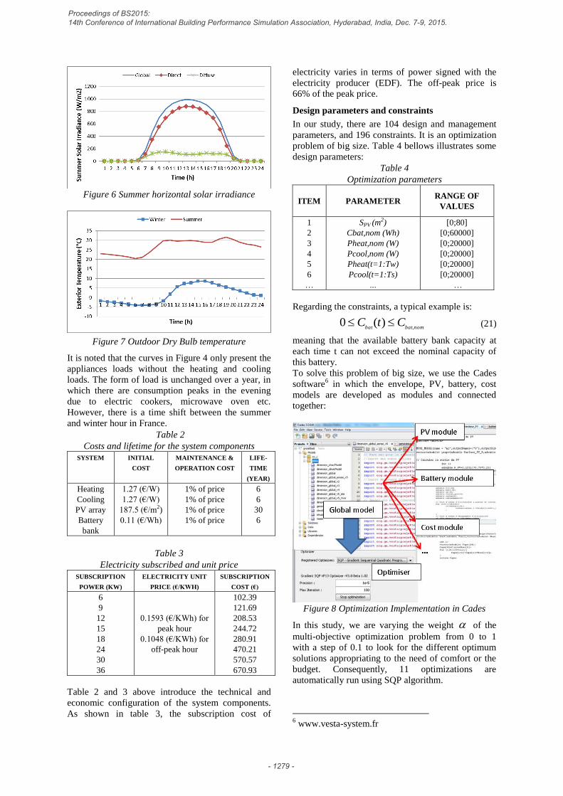
Figure 6 Summer horizontal solar irradiance
Figure 7 Outdoor Dry Bulb temperature
It is noted that the curves in Figure 4 only present the
appliances loads without the heating and cooling
loads. The form of load is unchanged over a year, in
which there are consumption peaks in the evening
due to electric cookers, microwave oven etc.
However, there is a time shift between the summer
and winter hour in France.
Table 2
Costs and lifetime for the system components
SYSTEM
INITIAL
COST
MAINTENANCE &
OPERATION COST
LIFE-
TIME
(YEAR)
Heating
Cooling
PV array
Battery
bank
1.27 (€/W)
1.27 (€/W)
187.5 (€/m2)
0.11 (€/Wh)
1% of price
1% of price
1% of price
1% of price
6
6
30
6
Table 3
Electricity subscribed and unit price
SUBSCRIPTION
POWER (KW)
ELECTRICITY UNIT
PRICE (€/KWH)
SUBSCRIPTION
COST (€)
6
9
12
15
18
24
30
36
0.1593 (€/KWh) for
peak hour
0.1048 (€/KWh) for
off-peak hour
102.39
121.69
208.53
244.72
280.91
470.21
570.57
670.93
Table 2 and 3 above introduce the technical and
economic configuration of the system components.
As shown in table 3, the subscription cost of
electricity varies in terms of power signed with the
electricity producer (EDF). The off-peak price is
66% of the peak price.
Design parameters and constraints
In our study, there are 104 design and management
parameters, and 196 constraints. It is an optimization
problem of big size. Table 4 bellows illustrates some
design parameters:
Table 4
Optimization parameters
ITEM
PARAMETER RANGE OF
VALUES
1
2
3
4
5
6
…
SPV (m2)
Cbat,nom (Wh)
Pheat,nom (W)
Pcool,nom (W)
Pheat(t=1:Tw)
Pcool(t=1:Ts)
…
[0;80]
[0;60000]
[0;20000]
[0;20000]
[0;20000]
[0;20000]
…
Regarding the constraints, a typical example is:
nombatbatCtC
,)(0 (21)
meaning that the available battery bank capacity at
each time t can not exceed the nominal capacity of
this battery.
To solve this problem of big size, we use the Cades
software6 in which the envelope, PV, battery, cost
models are developed as modules and connected
together:
Figure 8 Optimization Implementation in Cades
In this study, we are varying the weight of the
multi-objective optimization problem from 0 to 1
with a step of 0.1 to look for the different optimum
solutions appropriating to the need of comfort or the
budget. Consequently, 11 optimizations are
automatically run using SQP algorithm.
6 www.vesta-system.fr
Proceedings of BS2015: 14th Conference of International Building Performance Simulation Association, Hyderabad, India, Dec. 7-9, 2015.
- 1279 -

RESULTS AND DISCUSSION Table 5
Optimization results
OPTIM
GLOBAL
COST
(€)
WINTER
MEAN
DISCOMFORT
(°C)
SUMMER
MEAN
DISCOMFORT
(°C)
Pheat,nom
(W)
Pcool,nom
(W)
SPV
(m2)
Cbat,nom
(Wh)
1 0 19572 2.56 4.30 0 0 0 0
2 0.1 19572 2.56 4.30 0 0 0 0
3 0.2 44576 0.69 2.62 1800 1461 26 17856
4 0.3 64753 0.33 0.84 2318 3402 43 21905
5 0.4 74061 0.22 0.28 2458 3574 50 28498
6 0.5 74571 0.21 0.26 2486 3621 51 28541
7 0.6 90135 0.006 0.02 4216 4590 63 34918
8 0.7 90295 0.001 0.0018 4298 4594 64 35371
9 0.8 91365 0 0 4313 4787 67 37508
10 0.9 91365 0 0 4313 4787 67 37508
11 1 91365 0 0 4313 4787 67 37508
Once optimiser runs, we obtain the result of 11
optimisations within a short time (1m55s). This short
time is due to the use of partial derivatives (e.g.
Delinchant et al., 2007) of the variables of interest in
relation to design parameters, including the dynamic
integration on one side. On the other side, it is due to
the use of a deterministic SQP algorithm exploiting
this information of the gradient.
Table 5 shows all design results according to the
weight . When the value of is equal to 0 (no
requirement of comfort ), the optimiser indicates that
no energy system is necessary. In constrast, the
heating, air-conditioning, PV and battery bank
system should be installed with the nominal capacity
of 4313 (W), 4787 (W), 67 (m2) and 37508 (Wh)
respectively for the maximal comfort.
For the other values of , the nominal capacity of
system components is shown in the last 4 columns of
Table 5. The columns 3, 4, 5 of this table present the
compromise between the thermal comfort and the
global cost, which can be graphically illustrated as
bellow:
Figure 9 Pareto curve
In Figure 9, we only see 6 results instead of 11
because some optimization results are very similar. It
is found that the more money we spend the more
comfort we receive in winter and summer. This
compromise can be also seen in the analysis of
desired temperature response.
Indeed, in winter, the building interior temperatures
in Figure 10 depend on the heating power in Figure
11 for different cases of .
Figure 10 Winter interior temperature with
1;3.0;0
Figure 11 Winter heating power with
1;3.0;0
With 0 , we do not provide the heating power,
the interior temperature is much lower than the set
point for all time of winter day. In other words, the
building is always in the situation of discomfort
during 24 hours. With 3.0 , the building
Proceedings of BS2015: 14th Conference of International Building Performance Simulation Association, Hyderabad, India, Dec. 7-9, 2015.
- 1280 -

temperature is heated thanks to a heating system of
2.3KW but the desired temperature is not still
completely satisfied. With 1 , a heating system
of 4.3KW produces more heating energy so that the
building interior temperature respects perfectly the
set point. As a result, we can see the different
solutions of heating system (cheap or expensive)
according to the need of comfort.
In summer, in the same way, we can find out the
trade-off between the comfort and the cost generated
by air conditioning system in Figure 12 and 13.
Furthermore, we would like to show another trade
off: investment cost and energy cost. For example,
we consider the case 3.0 (Figure 12 and 13).
Figure 12 Summer interior temperature with
1;3.0;0
Figure 13 Summer cooling power with
1;3.0;0
It is seen in Figure 13 that air conditioning system
(red curve) is turned on early in the morning (pre-
cooling) and not turn off when the heated zone inside
air temperature (Figure 12) is better than the desired
temperature (at 9h for instance). It causes a
consumption increase but helps to avoid a peak
power at the next time (at 14h for example), which
will require a big investment cost of system. When
the unit investment cost of cooling system is so small
in comparison to the electricity unit price, we will
undoubtedly obtain the bigger cooling size but
consume the smaller total energy.
Finally, the global system management strategy in
summer and winter can be presented in the figures
below.
Figure 14 Summer and winter electricity unit price
Figure 15 Summer management strategy with
3.0
Figure 16 Summer state of charge of battery with
3.0
In summer, the air conditioning system was nearly all
the time activated when PV is producing (Figure 15).
From 9h to 17h, all loads were covered by the
renewable energy generation (auto-production). In
the early morning, the battery was discharged to
provide the energy to the load. When the sun is
rising, the produced energy surplus is charged in the
battery. At the end of the day, the discharge state is
reestablished in order to mitigate the load peak. It is
observed in Figure 15 that at 20h the electricity
power bought from the grid was reduced from 10KW
(total load) to 5.9KW thanks to the discharge of
battery. Compared to Table 3 we see that the
optimization is done such that the subscription power
is the lowest (type of 6KW). It can be noticed that the
electricity was not bought at the off-peak hour on
account of battery bank sizing problem. An
assumption is made, we buy the electricity at the off-
peak hours, 3h-8h for example (Figure 14), the state
of charge of battery will be higher than the actual
Proceedings of BS2015: 14th Conference of International Building Performance Simulation Association, Hyderabad, India, Dec. 7-9, 2015.
- 1281 -
value (22KWh, Figure 16). As a consequence, the
nominal capacity of storage will have to be bigger to
ensure the battery operation, which takes a higher
investment cost so that the global cost can be more
expensive. Thus, a decrease of battery size is more
effective than buying electricity from the grid in off-
peak hours in this case.
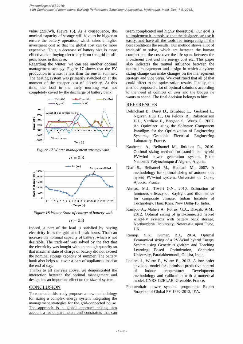
Regarding the winter, we can see another optimal
management strategy. Figure 17 shows that the PV
production in winter is less than the one in summer.
The heating system was primarily switched on at the
moment of the cheaper cost of electricity. At this
time, the load in the early morning was not
completely coved by the discharge of battery bank.
Figure 17 Winter management strategy with
3.0
Figure 18 Winter State of charge of battery with
3.0
Indeed, a part of the load is satisfied by buying
electricity from the grid at off-peak hours. That can
increase the nominal capacity of battery, which is not
desirable. The trade-off was solved by the fact that
the electricity was bought with an enough quantity so
that maximal state of charge of battery did not exceed
the nominal storage capacity of summer. The battery
bank also helps to cover a part of appliances load at
the end of day.
Thanks to all analysis above, we demonstrated the
interaction between the optimal management and
design has an important effect on the size of system.
CONCLUSION
To conclude, this study proposes a new methodology
for sizing a complex energy system integrating the
management strategies for the grid-connected house.
The approach is a global approach taking into
account a lot of parameters and constraints that can
seem complicated and highly theoretical. Our goal is
to implement it in tools so that the designer can use it
easily, and have all the tools for interpreting in the
best conditions the results. Our method shows a lot of
trade-off to solve, which are between the human
comfort and the cost over the life span, between the
investment cost and the energy cost etc. This paper
also indicates the mutual influence between the
optimal management and design in which a system
sizing change can make changes on the management
strategy and vice versa. We confirmed that all of that
could affect to the optimization results. Finally, this
method proposed a lot of optimal solutions according
to the need of comfort of user and the budget he
wants to spend. The final decision belongs to him.
REFERENCES
Delinchant B., Duret D., Estrabaut L., Gerbaud L.,
Nguyen Huu H., Du Peloux B., Rakotoarison
H.L., Verdiere F., Bergeon S., Wurtz F., 2007.
An Optimizer using the Software Component
Paradigm for the Optimization of Engineering
Systems, Grenoble Electrical Engineering
Laboratory, France.
Kaabeche A., Belhamel M., Ibtiouen R., 2010.
Optimal sizing method for stand-alone hybrid
PV/wind power generation system, Ecole
Nationale Polytechnique d’Algiers, Algeria.
Diaf S., Belhamel M., Haddadi M., 2007. A
methodology for optimal sizing of autonomous
hybrid PV/wind system, Université de Corse,
Ajaccio, France.
Ahmad, M.J., Tiwari G.N., 2010. Estimation of
luminous efficacy of daylight and illuminance
for composite climate, Indian Institute of
Technology, Hauz Khas, New Delhi-16, India.
Kamjoo A., Maheri A., Putrus, G.A., Dizqah, A.M.,
2012. Optimal sizing of grid-connected hybrid
wind-PV systems with battery bank storage,
Northumbria University, Newcastle upon Tyne,
UK.
Ramoji, S.K., Kumar, B.J., 2014. Optimal
Economical sizing of a PV-Wind hybrid Energy
System using Genetic Algorithm and Teaching
Learning Based Optimization, Centurion
University, Paralakhemundi, Odisha, India.
Leclere J., Wurtz F., Wurtz E., 2013. A low order
envelope model for optimised predictive control
of indoor temperature: Development
methodology and calibration with a numerical
model, CNRS-G2ELAB, Grenoble, France.
Photovoltaic power systems programme Report
Snapshot of Global PV 1992-2013, IEA.
Proceedings of BS2015: 14th Conference of International Building Performance Simulation Association, Hyderabad, India, Dec. 7-9, 2015.
- 1282 -