Optimal Retrospective Voting - University of Chicagohome.uchicago.edu/~bdm/PDF/retrospective.pdf ·...

Optimal Retrospective Voting∗

Ethan Bueno de Mesquita† Amanda Friedenberg‡

First Draft: August 11, 2005

Current Draft: July 12, 2006

Abstract

We argue that optimal retrospective voting can be thought of as an equilibrium selectioncriterion—specifically, a criterion that selects so as to maximize voter welfare. Formalized thisway, we go on to provide an informational rationale for retrospective voting. We show that aVoter can use retrospective voting to extract information from a Legislator with policy expertise.In particular, when the Voter’s strategy set is sufficiently rich, he can design a retrospectivevoting rule that ensures him expected payoffs as high as those he could achieve in the gamewhere he is a policy expert.

Keywords: Retrospective Voting, Political Economy, Electoral Control, Information ExtractionJEL Classification: D02, D72, D78, D81, D82

∗We are indebted to Randy Calvert for many conversations related to this project. We have also benefited fromcomments by Jim Alt, Heski Bar-Isaac, Adam Brandenburger, Catherine Hafer, Bard Harstad, Dimitri Landa, MottyPerry, Yuliy Sannikov, Jeroen Swinkels, and seminar participants at Berkely, Columbia, Hebrew University, andNYU. Bueno de Mesquita thanks the Center for the Study of Rationality, Political Science Department, and LadyDavis Fellowship, at Hebrew University for their hospitality and support.

†Department of Political Science, Washington University, 1 Brookings Drive, Campus Box 1063, St. Louis, MO63130, [email protected].

‡Olin School of Business, Washington University, 1 Brookings Drive, Campus Box 1133, St. Louis, MO 63130,[email protected]

Introduction

The political economy literature focuses on two accounts of voter behavior, retrospective andprospective voting. Retrospective voting is the idea that voters are backward-looking, conditioningtheir electoral decisions on politicians’ past performance without concern for their expected futureperformance (Key [17, 1966], Fiorina [15, 1981]). For instance, voters may reward politicians forhaving achieved economic growth or implemented environmental policies they like, even if suchoutcomes do not indicate a higher probability of similar outcomes in the future. Prospective votingis the idea that voters are forward-looking, conditioning their electoral decisions on expectationsabout the future (Kuklinski and West [18, 1981], Lewis-Beck [19, 1988], Lockerbie [21, 1992]). Forinstance, voters might support a politician because they believe that while in office, she will provideeconomic growth or environmental policies that benefit voters.

There is a long research tradition studying retrospective voting (see, for example, Key [17,1966], Barro [6, 1973], Fiorina [15, 1981], Ferejohn [14, 1986], Austen-Smith and Banks [5, 1989],Maskin and Tirole [22, 2004]). Moreover, retrospective voting has been supported empirically—i.e.,a variety of papers show that voters condition their electoral behavior on the past performance ofpoliticians. While some of this evidence is consistent with both retrospective and prospective voting(Lockerbie [20, 1991], Clarke and Stewart [10, 1995]), there is also direct evidence of backward-looking behavior (Alesina, Londregan and Rosenthal [1, 1993], Norpoth [25, 1996]).

This paper makes two contributions—one conceptual and one substantive. Conceptually, wesuggest that optimal retrospective voting is an equilibrium selection criterion. Substantively, weprovide an informational rationalle for retrospective voting. That is, we show that voters can useretrospective voting to extract information from politicians with policy expertise.

1 Optimal Retrospective Voting as Equilibrium Selection

What advantage do voters get from backward-looking behavior? An answer, dating back at least toV.O. Key, is that by threatening not to reelect politicians who perform poorly, voters can introducea degree of political accountability or electoral control.1 To borrow from Key (1966, page 77):

The odds are that the electorate as a whole is better able to make a retrospective ap-praisal of the work of governments than it is to make estimates of the future performanceof nonincumbent candidates. Yet by virtue of the combination of the electorate’s retro-spective judgement and the custom of party accountability, the electorate can exert aprospective influence if not control. Governments must worry, not about the meaningof past elections, but about their fate at future elections.

1There is also a literature that shows how past performance can convey information about expected future per-formance that prospective voters may use (Alesina and Rosenthal [2, 1995], Fearon [13, 1999], Persson and Tabellini[26, 2000], Ashworth [3, 2005], Besley [8, 2005]). We address that literature, and its critique of retrospective voting,in Section 3.

1

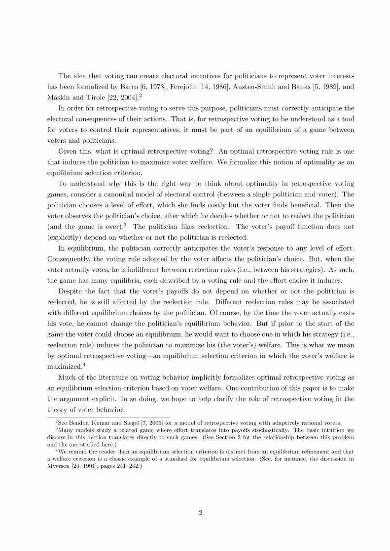
The idea that voting can create electoral incentives for politicians to represent voter interestshas been formalized by Barro [6, 1973], Ferejohn [14, 1986], Austen-Smith and Banks [5, 1989], andMaskin and Tirole [22, 2004].2

In order for retrospective voting to serve this purpose, politicians must correctly anticipate theelectoral consequences of their actions. That is, for retrospective voting to be understood as a toolfor voters to control their representatives, it must be part of an equilibrium of a game betweenvoters and politicians.

Given this, what is optimal retrospective voting? An optimal retrospective voting rule is onethat induces the politician to maximize voter welfare. We formalize this notion of optimality as anequilibrium selection criterion.

To understand why this is the right way to think about optimality in retrospective votinggames, consider a canonical model of electoral control (between a single politician and voter). Thepolitician chooses a level of effort, which she finds costly but the voter finds beneficial. Then thevoter observes the politician’s choice, after which he decides whether or not to reelect the politician(and the game is over).3 The politician likes reelection. The voter’s payoff function does not(explicitly) depend on whether or not the politician is reelected.

In equilibrium, the politician correctly anticipates the voter’s response to any level of effort.Consequently, the voting rule adopted by the voter affects the politician’s choice. But, when thevoter actually votes, he is indifferent between reelection rules (i.e., between his strategies). As such,the game has many equilibria, each described by a voting rule and the effort choice it induces.

Despite the fact that the voter’s payoffs do not depend on whether or not the politician isreelected, he is still affected by the reelection rule. Different reelection rules may be associatedwith different equilibrium choices by the politician. Of course, by the time the voter actually castshis vote, he cannot change the politician’s equilibrium behavior. But if prior to the start of thegame the voter could choose an equilibrium, he would want to choose one in which his strategy (i.e.,reelection rule) induces the politician to maximize his (the voter’s) welfare. This is what we meanby optimal retrospective voting—an equilibrium selection criterion in which the voter’s welfare ismaximized.4

Much of the literature on voting behavior implicitly formalizes optimal retrospective voting asan equilibrium selection criterion based on voter welfare. One contribution of this paper is to makethe argument explicit. In so doing, we hope to help clarify the role of retrospective voting in thetheory of voter behavior.

2See Bendor, Kumar and Siegel [7, 2005] for a model of retrospective voting with adaptively rational voters.3Many models study a related game where effort translates into payoffs stochastically. The basic intuition we

discuss in this Section translates directly to such games. (See Section 2 for the relationship between this problemand the one studied here.)

4We remind the reader than an equilibrium selection criterion is distinct from an equilibrium refinement and thata welfare criterion is a classic example of a standard for equilibrium selection. (See, for instance, the discussion inMyerson [24, 1991], pages 241–242.)

2

2 Electoral Control and Information Extraction

We provide a new substantive insight into the study of retrospective voting. In particular, we showthat voters can use retrospective voting both to control politicians and to extract information frompoliticians with policy expertise.

In many existing models of retrospective voting, the focus is on giving a politician incentivesto take a costly action: in Barro [6, 1973] and Ferejohn [14, 1986], this is on an “effort” dimension,and in Austen-Smith and Banks [5, 1989], this is on a “policy” dimension. Any uncertainty isabout the politician’s actions, not about the voter’s preferences over policy outcomes. That is, inthese models the voter knows what he wants (high effort) but not what the politician did. As such,the optimal retrospective voting rule has features familliar from the canonical model of contractingunder moral hazard.

Yet, in many interesting settings, politicians are policy experts relative to voters. That is, thepolitician’s private information is about the likely impact of policies. This type of information mayinfluence the voter’s preferences over policy outcomes. Here, the voter knows what the politiciandid (the policy she chose) but not what he (the voter) wants.5 In this environment, the challengein designing an optimal retrospective voting rule is that the voter does not know in advance whatbehavior he wants to induce.

One conjecture is that, when the voter is uncertain about his preferences (i.e., his most preferredpolicy or “ideal point”), the optimal retrospective voting rule would at best result in the politicianchoosing the voter’s expected ideal point. After all, this is the policy the voter himself wouldimplement, if he were empowered to choose policy directly. We show that the voter can alwaysdesign a retrospective voting rule that provides higher payoffs than this. Since the voter could nothave done so well on his own, he must be extracting information from the politician.

The level of information extraction that the voter can achieve depends on how rich his strategyset is. We allow this richness to vary in two ways.

First, we restrict the voter to pure strategies but allow for the possibility that, after the policyis chosen, the voter may become informed of the true state. We show that even if the voter only hasa fifty-fifty chance of learning the true state, he can design a retrospective voting rule that ensureshim expected payoffs as high as those he could achieve in a game where he is perfectly informed.That is, the voter achieves full information extraction.

Second, we allow the voter to employ mixed strategies. Here we show that even if the voter hasno chance of ever learning the true state directly, he can nonetheless design a retrospective votingrule that extracts full information.

These information extraction results are surprising because they show that the voter’s lack ofinformation comes at no cost to him. Even when the voter has a significant level uncertainty, hecan still induce the legislator to choose his ideal point in the same set of states he could whenperfectly informed.

5We thank Motty Perry for suggesting this turn of phrase.

3

We provide tight characterizations of the optimal retrospective voting rule. For instance, wewill see that, in pure strategies, the optimal rule always takes one of two forms, regardless of theprobability that the voter learns the true state.

It is worth noting that Maskin and Tirole [22, 2004] also study a game in which the politicianhas private information that influences the voters’ preferences. However, they focus on a differentset of issues and so a different game. There, voting not only serves to control politicians, but also toselect politicians with the same preferences as the voter. If the politician’s preferences are alignedwith the voter’s, the voter’s electoral control and information extraction problems disappear. Here,we show that in a wide variety of circumstances, voters can solve the problems of electoral controland information extraction for a given preference ranking of the legislator. Put differently, to solvethese problems, voters need not select a legislator whose preferences are aligned with their own.

3 Is Retrospective Voting Ever Optimal?

We formalize optimal retrospective voting as an equilibrium selection criterion and provide an infor-mational rationalle for retrospective voting. Together, these two points provide a new perspectiveon a common critique of restrospective voting.

Critics have argued that, while voters would like to adopt retrospective voting rules that givepoliticians optimal incentives, such rules are not credible. At the point when voters actuallyvote, their electoral decisions do not affect politicians’ past actions. Thus, rational voters cannotcredibly commit to voting rules for the purpose of providing incentives. Instead, they must beforward-looking, electing politicians who can be expected to deliver the highest payoffs in thefuture (Alesina and Rosenthal [2, 1995], Fearon [13, 1999], Besley [8, 2005]).

We believe that even forward-looking voters can adopt retrospective voting aimed at electoralcontrol and information extraction. Retrospective and prospective voting are not mutually exclu-sive. Rather, they are complementary considerations. We justify this claim in two ways.

First, recall that we formalize optimal retrospective voting as an equilibrium selection criterion.As long as voters are selecting from the set of sequentially rational equilibria, their retrospectivevoting rule is credible—there is no commitment problem. Thus, when conceived of in terms ofequilibrium selection, the rationale for retrospective voting is independent of and does not conflictwith sequential rationality.6

Of course, equilibrium selection is interesting only if the game has multiple sequentially rationalequlibria. While many extant models have a unique equilibrium, this is largely due to their adoptinga stylized approach to highlight their substantive results. For example, these models generallyassume that legislative outputs are a simple combination of “ability” and “effort” (Persson andTabellini [26, 2000], Ashworth [3, 2005], Besley [8, 2005]). Small changes to such models (e.g.,adding a policy dimension or richer electoral or institutional environments) can give rise to multiple

6For a different argument that retrospective and prospective motivations are not mutually exclusive, as well as aformal model in which both types of motivation arise endogenously, see Snyder and Ting [27, 2005].

4

equilibria, even with forward-looking voters (see, for example, Ashworth and Bueno de Mesquita[4, 2006]).

Second, beyond the issue of multiplicity, it is not clear that the commitment problem arisesin all interesting voting games. In some settings, it is natural to assume that voters learn aboutfactors (i.e., their representatives’ ability or trustworthiness) that affect their future payoffs. This isparticularly true in the sort of effort games (without information extraction) that the literature hastended to focus on. For instance, in models of constituency service or local public goods provision,a legislator’s individual characteristics are likely to be important. However, other settings do notnaturally suggest this type of learning. This is particularly true in the sort of games with policyexpertise that we focus on. For example, if the voters already know her policy preferences, thenhow a legislator votes on purely ideological (environmental policy or gay marriage) or redistributiveissues is unlikely to communicate information about her inherent characteristics.7 In such settings,observations of legislative action may not affect voters’ beliefs about likely future performance.Hence, no commitment problem arises.

Given these arguments, we believe that there are good reasons to study retrospective votingas an independent rationale for why voters condition on observations of past performance. Tothis end, we study a simple game of policy choice and elections in which there are no prospectiveconcerns. (The game ends after the election.) This allows us to focus on how retrospective votingcan be used both to extract information and to discipline legislators, abstracting away from anyprospective incentives.

4 Primitives

There are two players, the Legislator and the Voter. We refer to the Legislator as “she” and theVoter as “he.” The order of play is as follows. Nature chooses a state, which determines theVoter’s policy preferences. The Legislator observes the true state and then chooses a policy. Afterthis, Nature chooses whether or not to inform the Voter of the true state. The Voter observes theLegislator’s policy choice and then decides whether or not he will reelect the Legislator.8

The set of states, viz. Ω, is a topological space. Then (Ω,A, µ) is a measure space, where A isthe Borel sigma-algebra and µ is the Voter’s prior. The set of policies is the real line. Write p ∈ Rfor a given policy. Nature chooses ι from i, ni, where i represents the decision to inform the Voterof the true state of the world and ni represents the decision not to inform the Voter of this state. Itis ‘transparent’ to the players that Nature chooses the action ‘inform’ with probability π ∈ [0, 1].9

Reelection is a choice r from 0, 1, where r = 0 represents the Voter’s decision not to reelect the7Under our analysis, it is without loss of generality to assume that there is no uncertainty about the Legislator’s

policy preferences. (See the Online Appendix for a formal treatment.) So, even if the Voter is uncertain about theLegislator’s policy preferences, there is a role for retrospective voting as a selection criterion.

8We do not explicitly include a challenger. Our game does not include a future in order to focus on the use ofretrospective voting to provide incentives. As such, including a challenger (who may or may not be ex ante identicalto the incumbent) would have no affect on the analysis.

9By ‘transparent’ we mean what is colloquially referred to as ‘common knowledge.’

5

Legislator. The Legislator’s policy preferences do not vary with the state. In particular, normalizethe Legislator’s ideal point to 0, for every state. (See Section 8.3 for an extension to the case wherethe Legislator’s ideal point depends on the state.)

Let xv : Ω → R be a surjective real-valued random variable. The interpretation is that xv (ω)is the Voter’s ideal point when the true state is ω. Since the mapping is surjective, for anypolicy p there exists some state ω such that p is the Voter’s ideal point at ω. The Legislator hasquadratic preferences over policy and seeks reelection. Given a policy p and an ideal point of 0,the Legislator gains a payoff −p2. (Our results do not hinge on quadratic payoffs. See Section8.1.) If reelected, the Legislator receives a payoff of B > 0. Taken together, these imply that theLegislator’s extensive-form payoff function is ul : R× 0, 1 → R, where

ul(p, r) = −p2 + rB.

For each state, the Voter has quadratic preferences over policy. Formally, the Voter’s extensive-formpayoff function is uv : Ω× R→ R, where

uv(ω, p) = − (p− xv (ω))2 .

The extensive form described above induces a strategic form. A strategy for the Legislator is amap from states to policies, viz. sl : Ω → R. A strategy for the Voter is a map sv : Ω×R×i, ni →0, 1, where for every policy p and all states ω, ω′ ∈ Ω, sv (ω, p, ni) = sv (ω′, p, ni). That is, if theVoter is uninformed, the true state cannot affect his action. Let Sl (resp. Sv) be the set of purestrategies for the Legislator (resp. Voter). With this, we can specify strategic-form payoff functions,viz. Ul : Ω× i, ni × Sl × Sv → R and Uv : Ω× Sl → R, with

Ul (ω, ι, sl, sv) = ul (sl (ω) , sv (ω, sl (ω) , ι)) = −sl (ω)2 + sv (ω, sl (ω) , ι) B

Uv (ω, sl) = uv (ω, sl (ω)) = − (sl (ω)− xv (ω))2.

Write Eul (p, sv (ω, p, ι)) for the expected payoffs of the Legislator with respect to ι ∈ i, ni, i.e.,

Eul (p, sv (ω, p, ι)) = πul (p, sv (ω, p, i)) + (1− π) ul (p, sv (ω, p, ni)) .

4.1 Equilibrium

The role of retrospective voting is to induce the Legislator to take actions that are beneficial tothe Voter. That is, if the Voter’s actions are responsive to policy, then the Legislator shouldtake this into account when choosing policy. This requires that the Legislator correctly anticipatehow the Voter will respond to her choice of policy. Therefore, studying this role of retrospectivevoting suggests restricting attention to a solution concept where players’ beliefs are correct, namelyequilibrium.

For now, we will restrict attention to pure-strategy Bayesian Equilibrium. In Section 7, we

6

allow players to make use of behavioral strategies. (From here until Section 7, anytime we refer tothe term Bayesian Equilibrium, we mean a pure-strategy Bayesian Equilibrium.)

Definition 4.1 A pair (s∗l , s∗v) is a pure-strategy Bayesian Equilibrium if:

(i) s∗l is measurable;

(ii) for each ω ∈ Ω, Eul (s∗l (ω) , s∗v (ω, s∗l (ω) , ι)) ≥ Eul (p, s∗v (ω, p, ι)) for all p ∈ R.

The first requirement is that the Voter must be able to calculate his expected payoffs. For this,s∗l must be measurable. Because the Voter makes his reelection decision at the end of the game,his choice does not directly affect his payoffs. As such, an explicit optimization requirement for theVoter is omitted.10 The second requirement is that, at each state, the Legislator must choose apolicy that maximizes her expected payoffs, given the Voter’s actual reelection rule.

4.2 Optimal Retrospective Voting

Thus far, we have not considered a non-trivial optimization problem for the Voter. In a BayesianEquilibrium, at each state, the Legislator chooses an optimal policy given the actual electoralstrategy s∗v. But, at the time that the Voter makes his reelection decision, he is indifferent amongall strategies. That said, given that in a Bayesian Equilibrium the Legislator correctly anticipatesthe Voter’s actual electoral strategy, there is a sense in which the Voter has an optimal reelectionrule. In particular, an optimal retrospective voting rule is one the Voter would choose if he couldsurvey the Legislator’s best responses for each reelection rule and choose an equilibrium in whichhis welfare is maximized.

Put differently, optimal retrospective voting identifies the Voter’s most preferred equilibria fromthe set of all Bayesian Equilibria. Notice, for any given strategy of the Voter, the Legislator mayhave multiple best responses. Thus, there may be multiple equilibria associated with any givenVoter strategy. Optimal retrospective voting selects a pair of Voter and Legislator equilibriumstrategies that maximizes the Voter’s welfare.

It is important to note that, in equilibrium, the Legislator correctly anticipates the Voter’sresponse to policy choice. As such, a feature of an equilibrium analysis (as per Definition 4.1) isthat the Voter’s actual reelection rule influences the Legislator’s behavior. We do not say howor why players might arrive at playing an equilibrium. So, in particular, we do not require thatthe Voter ‘announce’ or ‘commit’ to a strategy before the game is played. Of course, we do notrule out that ‘announcement’ or ‘commitment’ can lead to equilibrium play. The point is simplythat, in any equilibrium-based solution concept, the Voter’s actual strategy choice influences theLegislator’s behavior.11

10For the same reason, we omit a requirement on updating beliefs. Imposing the natural requirement yields anequivalent definition.

11This need not be the case for a non-equilibrium solution concept, e.g., rationalizability.

7

Just as we do not say how players arrive at an equilibrium, we do not say how players arriveat an equilibrium that maximizes the Voter’s welfare. Indeed, one need not view the equilibriumselection as a behavioral prediction at all. Rather, we are interested in identifying the best possibleoutcome the Voter can hope to achieve through retrospective voting. (Again, just as we do notrule out that that ‘announcement’ or ‘commitment’ may lead to equilibrium play, we do not ruleout that it could lead to a specific equilibrium.)

We need to specify the Voter’s “most preferred” equilibrium. We formalize this with the fol-lowing two selection criteria:

Definition 4.2 A strategy profile (s∗l , s∗v) is an Expectationally Optimal Equilibrium if it is

a Bayesian Equilibrium and, for all Bayesian Equilibria (sl, sv),

∫

Ωuv (ω, s∗l (ω)) dµ ≥

∫

Ωuv (ω, sl (ω)) dµ.

Definition 4.3 A strategy profile (s∗l , s∗v) is a State-by-State Optimal Equilibrium if it is a

Bayesian Equilibrium and there does not exist a Bayesian Equilibrium (sl, sv) with

uv (ω, sl (ω)) ≥ uv (ω, s∗l (ω)) for all ω ∈ Ωuv (ω, sl (ω)) > uv (ω, s∗l (ω)) for some ω ∈ Ω.

A strategy profile (s∗l , s∗v) is Expectationally Optimal if, among all Bayesian Equilibria, (s∗l , s

∗v)

maximizes the Voter’s expected payoffs given the prior µ. Alternatively, if (s∗l , s∗v) is State-by-State

Optimal, then there does not exist a Bayesian Equilibrium, viz. (sl, sv), where (i) for every stateω ∈ Ω, the Voter’s payoff under (sl, sv) is at least as great as his payoff under (s∗l , s

∗v) and (ii) there

exists a state ω ∈ Ω where the Voter’s payoff under (sl, sv) is strictly greater than his payoff under(s∗l , s

∗v). In Section 8.2, we discuss these criteria and explain why they are distinct.

Before continuing, it will be useful to define some loose terminology. Fix two strategy profiles(sl, sv) and (s∗l , s

∗v). If either

∫Ω uv (ω, sl (ω)) dµ >

∫Ω uv (ω, s∗l (ω)) dµ or the strategy profiles satisfy

the conditions in the display of Definition 4.3, we will say “the Voter strictly prefers (sl, sv) to(s∗l , s

∗v).”

5 Benchmark Result

Here, we analyze a simple version of the game, one in which it is transparent to the players thatNature chooses not to inform the Voter (i.e., π = 0). Even in this case, the Voter can extractinformation.

This version of the game can be translated into one in which Nature must choose not to informthe Voter about the true state. Under that specification, the Voter’s strategy need not specifyan action when Nature chooses to inform him. Therefore, we restrict the domain of the Voter’sstrategy sv to be Ω × R × ni. Since the true state cannot affect the Voter’s action when he isuninformed, we can suppress reference to ω and ι = ni. That is, write sv (p) for sv (ω, p, ni).

8

It will be convenient to begin by characterizing the set of Bayesian Equilibria for this game.Two principles will aid in the characterization. First, by choosing p = 0, the Legislator can assureherself a payoff of at least zero. Thus, the Voter can never induce the Legislator to choose policiesthat are further than

√B from the Legislator’s ideal point. Second, if multiple policies will be

rewarded with reelection, the Legislator never has an incentive to choose any but the policy closestto her ideal point. Given these facts, the following characterization follows.12

Proposition 5.1 If (sl, sv) is a Bayesian Equilibrium, then it must take one of the following forms:

(i)

(a) sl (ω) = 0 for all ω ∈ Ω

(b) sv (p) = 0 for all p ∈ [−√B,√

B],

(ii) there exists B > p ≥ 0 where, for all p ∈ (−p, p), sv (p) = 0 and

(a) sl (ω) ∈ −p, p for all ω ∈ Ω

(b) sv (sl (ω)) = 1 for all ω ∈ Ω,

(iii) for all p ∈ (−√B,√

B), sv (p) = 0 and

(a) sl (ω) ∈ 0,−√B,√

B for all ω ∈ Ω

(b) sv (sl (ω)) = 1 for all sl (ω) ∈ −√B,√

B.

Part (i) says that if the Voter does not reward any policies within√

B of the Legislator’s idealpoint, then the Legislator chooses her ideal point at every state. For Parts (ii)–(iii), consider theset of policies the Voter rewards with reelection. In particular, let −p and p ≥ 0 be the policiesclosest to the Legislator’s ideal point that the Voter rewards with reelection. Part (ii) considers thecase where −p and p lie strictly within

√B of the Legislator’s ideal point. Here, the Legislator’s

best response is to choose either of −p or p. Part (iii) considers the case where p =√

B. Since theVoter rewards −p or p with reelection, the Legislator is indifferent between choosing these policiesand her ideal point.

5.1 Optimal Retrospective Voting in the Benchmark Case

Were the uninformed Voter empowered to choose policy, maximizing his expected payoffs wouldrequire that he choose his expected ideal point. (See Lemma A6.) However, the Voter cannotchoose policy. Rather, the Legislator is his agent. One conjecture is that this agency relationshipleaves the Voter worse off relative to choosing policy himself. In particular, when the Legislator’sand Voter’s preferences diverge sufficiently, the Voter cannot offer the Legislator sufficient electoralincentives to choose his ideal point.

12The proof of this and all subsequent results can be found in the appendices.

9

BB− ( )vE x( )vE x− 0

( ) ( )If 0, choose v vx E xω < − ( ) ( )If 0, choose v vx E xω ≥

Figure 5.1: A legislative choice that improves the voter’s expected utility relative to always choosinghis expected ideal point.

But there is another important aspect of this game. In particular, the Legislator is informed ofthe true state. As such, while the Voter does not know his ideal point, the Legislator does. Thechallenge for the Voter is to use electoral incentives to extract this information from the Legislatorin a way that improves his expected payoffs.

How can the Voter extract such information? Suppose that the Voter could induce the Legislatorto choose his expected ideal point, viz. E (xv). Refer to Figure 5.1 and suppose that E (xv) > 0.Proposition 5.1 suggests that he can also induce the Legislator to choose −E (xv). Indeed, becausethe Legislator’s ideal point is zero, she must be indifferent between (i) choosing E (xv) and beingreelected and (ii) choosing −E (xv) and being reelected. This indicates that the Voter can dobetter than simply inducing the Legislator to choose his expected ideal point. In particular, thereis an equilibrium where the Legislator chooses E (xv) when the Voter’s ideal point is positive and−E (xv) when the Voter’s ideal point is negative.

More precisely, the Voter will strictly prefer a moderate two-sided voting rule: the Voter reelectsthe Legislator if and only if she chooses either −p∗ or p∗. The Legislator chooses the policy p∗ ≥ 0when the Voter’s ideal point is positive and otherwise chooses the policy −p∗. Let Ω+ be theset of states where the Voter’s ideal point is positive, viz. ω : xv (ω) ≥ 0. Under ExpectationalOptimality, the Voter selects this voting rule so that p∗ ≥ 0 maximizes

−∫

Ω+

(xv (ω)− p)2 dµ (ω)−∫

Ω\Ω+

(xv (ω) + p)2 dµ(ω)

subject to p ∈ [−√

B,√

B].

This policy p∗ will be given by

p∗ =∫

Ω+

xv (ω) dµ (ω)−∫

Ω\Ω+

xv (ω) dµ (ω) ≥ 0,

when this value is in [0,√

B], and√

B otherwise. (See Proposition 5.2 below.)Consider the example in Figure 5.2. Here Ω = R and xv is the identity map. Let µ be the

uniform distribution on [−√B,√

B]. Since the distribution is symmetric, p∗ is the expected valueof the Voter’s ideal point, conditional on the ideal point being positive, i.e., p∗ =

√B2 .

10

Reelect if and only if

B- B 12 B

12- B 0

Choose12 BChoose

12- B

Figure 5.2: A moderate two-sided voting rule.


B- B B32B3

2- 12 B

12- B 0

Choose - B Choose BChoose 0

Figure 5.3: An extreme two-sided voting rule.

A moderate two-sided voting rule need not be Expectationally Optimal. To see this, continueto assume that Ω = R and xv is the identity map. Now, let µ be the uniform distribution on[−3

2

√B, 3

2

√B]. The policy p∗ = 3

4

√B maximizes the Voter’s expected payoffs given all moderate

two-sided voting rules. The Voter’s expected payoffs are −38

√B.

However, the Voter can obtain higher expected payoffs. Consider instead the following extremetwo-sided voting rule, illustrated in Figure 5.3: the Voter reelects the Legislator if and only if shechooses a policy of either −√B or

√B. The Legislator (i) chooses her ideal point (zero) when the

Voter’s ideal point is contained in [−12

√B, 1

2

√B], (ii) chooses the policy −√B when the Voter’s

ideal point is strictly less than −12

√B, and (iii) otherwise chooses

√B. Under this voting rule, the

Voter’s expected payoffs are −14

√B. So this voting rule yields strictly higher expected payoffs for

the Voter than any moderate two-sided voting rule.An extreme two-sided voting rule is indeed a Bayesian Equilibrium. (See Lemma A8.) Intu-

itively, at any state, the Legislator is choosing a policy among 0,−√B,√

B. The policies −√B

and√

B are rewarded with reelection and so yield the Legislator a payoff of zero, at any state. Thepolicy zero is not rewarded with reelection. So, at any state, the Legislator is indifferent betweenchoosing any one of these policies.

Under this voting rule, when the Voter’s ideal point lies in [−12

√B, 1

2

√B] and the Legislator

chooses the policy zero, the Legislator does not get reelected. Thus, there is a sense in which theVoter punishes the Legislator for choosing the policy he wants her to choose. This is no coincidence.If the Voter were to reward the Legislator with reelection when she chooses her ideal point, then

11

the Legislator would never choose the policies −√B or√

B. In order to induce the Legislator tochoose policies close to the Voter’s ideal point when this ideal point is extreme, the Voter cannotreward the Legislator with reelection for choosing centrist policies.

Similarly, an extreme two-sided voting rule cannot involve the Legislator being rewarded forchoosing some policy p ∈ (0,

√B). If it did, at any state, the Legislator would strictly prefer to

choose this policy to her own ideal point. Thus, in order to induce the Legislator to choose policiesclose to the Voter’s ideal point when that ideal point is close to zero, the Voter does not rewardany p ∈ (0,

√B) with reelection.

These examples illustrate two possible types of optimal retrospective voting rules. What differ-entiates situations in which optimal retrospective voting will involve a moderate versus an extremetwo-sided voting rule? Under the extreme two-sided rule, the policy the Legislator must choosein order to be reelected is more extreme than under the moderate two-sided rule. In the secondexample, the Voter’s beliefs placed greater probability on his ideal point being further from zero.This is why the Voter favored the extreme two-sided rule.

We now turn to the characterization of the optimal retrospective voting rule in this benchmarkcase. It will be useful to first formally define moderate and extreme two-sided voting rules.

Definition 5.1 Fix a policy p∗

p∗ =∫

Ω+


Ω\Ω+

xv (ω) dµ (ω) .

Say (s∗l , s∗v) is a moderate two-sided voting rule if p∗ ∈ (0,

√B) and the following are satisfied:

(i) s∗l (ω) = −p∗ whenever xv (ω) < 0, s∗l (ω) = p∗ whenever xv (ω) > 0, and s∗l (ω) ∈ −p∗, p∗whenever xv (ω) = 0;

(ii) if p ∈ [−p∗, p∗], then s∗v (p) = 1 if and only if p ∈ −p∗, p∗.

Definition 5.2 Say (s∗l , s∗v) is an extreme two-sided voting rule if the following are satisfied:

(i) s∗l (ω) = 0 whenever xv (ω) ∈ (−12

√B, 1

2

√B), s∗l (ω) = −√B whenever xv (ω) < −1

2

√B,

s∗l (ω) =√

B whenever xv (ω) > 12

√B, s∗l (ω) ∈ −√B, 0 whenever s∗l (ω) = −1

2

√B, and

s∗l (ω) ∈ 0,√

B whenever s∗l (ω) = 12

√B;

(ii) if p ∈ [−√B,√

B], then s∗v (p) = 1 if and only if p ∈ −√B,√

B.

Proposition 5.2 There exists an Expectationally and State-by-State Optimal Equilibrium. Anysuch equilibrium is either a moderate or an extreme two-sided voting rule.

Proposition 5.2 establishes that an optimal retrospective voting rule will take one of two simpleforms, namely a moderate or an extreme two-sided voting rule. When the Voter’s expected idealpoint lies within

√B of zero, he strictly prefers an optimal retrospective voting rule to choosing

12

his expected ideal point at every state. This is one sense in which the Voter can use retrospectivevoting to extract information from the Legislator.

But notice that there are only limited circumstances in which the policies chosen coincide withthe Voter’s actual ideal point. (In the case of a moderate two-sided voting rule associated withpolicy p∗, this will be the set of states (xv)

−1 (−p∗, p∗). For an extreme two-sided voting rule, itis the set (xv)

−1 (0,−√B,√

B).)It will turn out that the Voter can only extract a limited amount of information because his

strategy set is not sufficiently rich. The next two sections enrich the Voter’s strategy set in twoways. In Section 6, we allow for the possibility that the Voter may learn the true state afterthe Legislator chooses the policy. Here, we give conditions under which the Voter achieves fullinformation extraction. In Section 7, we allow the Voter to make use of behavioral strategies.Here, we show that—even when there is no chance that the Voter will learn the true state—he cannonetheless achieve full information extraction.

6 Enriching the Strategy Set: Partially Informed Voter

Contrast the Benchmark specification with the case where it is transparent that Nature alwaysinforms the Voter (i.e., π = 1). Here, the Voter can condition reelection on both the policy andstate. In particular, the Voter can choose a voting rule where, for each state ω, he reelects theLegislator if and only if she chooses his ideal point xv (ω). When the Voter’s ideal point is within√

B of zero, such a voting rule will induce the Legislator to choose this ideal point.In the case where the Voter is fully informed, there is no need to extract information from

the Legislator. The fact that the Voter can induce the Legislator to choose his ideal point doesnot reflect information extraction. Rather, it reflects ‘leverage’ over the Legislator due to the factthat the Voter can condition reelection on his actual ideal point. That is, it reflects a richer set ofstrategies.

Now, consider a game in which it is transparent that the Voter learns the true state with someprobability π ∈ (0, 1). Here, the Voter still has some ‘leverage,’ i.e., a richer set of strategies.But unlike the case where the Voter is fully informed, there is some positive probability that theVoter will never learn the true state. There are two implications of this. First, while, in principle,the Voter can condition reelection on the true state, he may not be able to do so in practice—his‘informed information set’ may not be reached. Second, the Voter would like to use retrospectivevoting for both electoral control and information extraction. Can the Voter use the gained ‘leverage’to extract additional information?

It turns out the answer is yes. To gain an intuition for why, we will begin by looking at aretrospective voting rule that is analogous to the extreme two-sided rule in the Benchmark case(π = 0). We will see how the Voter can use his additional ‘leverage’ to alter this rule and improvehis expected payoffs.

13

If ∉ Φ, reelect if and only if

B- B Bπ- Bπ 0

Choose BChoose - B Choose Voter's Ideal Point

Reelect if ω ∈ Φand informed

Figure 6.1: Modifying an extreme two-sided voting rule.

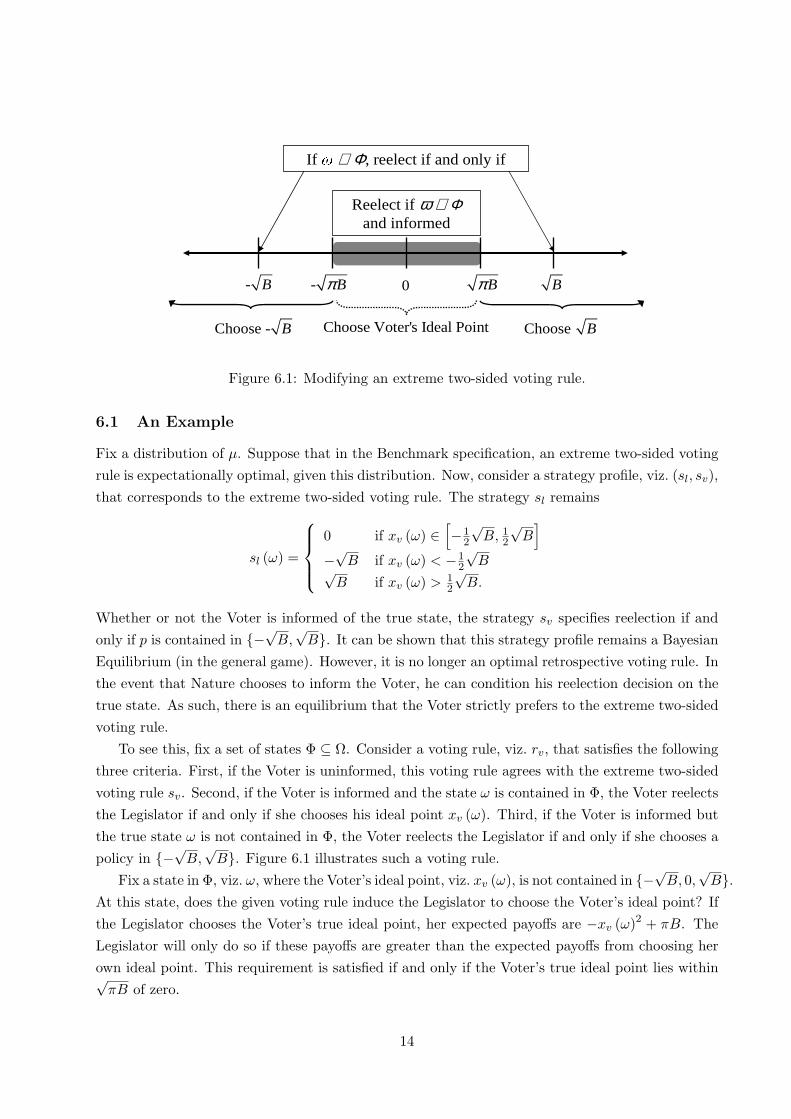
6.1 An Example

Fix a distribution of µ. Suppose that in the Benchmark specification, an extreme two-sided votingrule is expectationally optimal, given this distribution. Now, consider a strategy profile, viz. (sl, sv),that corresponds to the extreme two-sided voting rule. The strategy sl remains

sl (ω) =

0 if xv (ω) ∈[−1

2

√B, 1

2

√B

]

−√B if xv (ω) < −12

√B√

B if xv (ω) > 12

√B.

Whether or not the Voter is informed of the true state, the strategy sv specifies reelection if andonly if p is contained in −√B,

√B. It can be shown that this strategy profile remains a Bayesian

Equilibrium (in the general game). However, it is no longer an optimal retrospective voting rule. Inthe event that Nature chooses to inform the Voter, he can condition his reelection decision on thetrue state. As such, there is an equilibrium that the Voter strictly prefers to the extreme two-sidedvoting rule.

To see this, fix a set of states Φ ⊆ Ω. Consider a voting rule, viz. rv, that satisfies the followingthree criteria. First, if the Voter is uninformed, this voting rule agrees with the extreme two-sidedvoting rule sv. Second, if the Voter is informed and the state ω is contained in Φ, the Voter reelectsthe Legislator if and only if she chooses his ideal point xv (ω). Third, if the Voter is informed butthe true state ω is not contained in Φ, the Voter reelects the Legislator if and only if she chooses apolicy in −√B,

√B. Figure 6.1 illustrates such a voting rule.

Fix a state in Φ, viz. ω, where the Voter’s ideal point, viz. xv (ω), is not contained in −√B, 0,√

B.At this state, does the given voting rule induce the Legislator to choose the Voter’s ideal point? Ifthe Legislator chooses the Voter’s true ideal point, her expected payoffs are −xv (ω)2 + πB. TheLegislator will only do so if these payoffs are greater than the expected payoffs from choosing herown ideal point. This requirement is satisfied if and only if the Voter’s true ideal point lies within√

πB of zero.

14

B- B Bπ- Bπ 0

Choose Voter's Ideal Point

Figure 6.2: Informed incentives.

So, suppose that the Voter chooses Φ to be the set of states where his ideal point is containedin [−√πB,

√πB], i.e., Φ = (xv)

−1 ([−√πB,√

πB]). The above arguments suggest the following:the strategy profile (rl, rv) is a Bayesian Equilibrium, where (i) rl (ω) = xv (ω) when xv (ω) ∈[−√πB,

√πB] and (ii) rl (ω) = sl (ω) otherwise. When the Voter’s true ideal point is contained in

[−√πB,√

πB]\ 0, his payoffs under (rl, rv) are strictly greater than his payoffs under the extremetwo-sided voting rule (sl, sv). In other cases, the payoffs agree. So, an extreme two-sided rule is nolonger State-by-State Optimal.

6.2 Informed vs. Uninformed Incentives

Return to the example in Section 6.1 above. There we constructed a Bayesian equilibrium, viz.(rl, rv), that the Voter strictly prefers to the extreme two-sided voting rule (sl, sv). We will seethat even this voting rule is not an optimal retrospective voting rule. To see this, we will point totwo types of incentives the strategy rv offers: informed and uninformed incentives.

Begin with informed incentives. Say the Voter offers informed incentives to choose policy p ata state ω, if the Voter’s strategy takes the following form: if the true state is ω and the Voter isinformed, he reelects the Legislator if and only if she chooses policy p. Returning to the example,rv offers informed incentives to choose the Voter’s ideal point at any state ω ∈ Φ.

At a given state, can the Voter use informed incentives (alone) to induce the Legislator to choosehis ideal point? If the Voter’s and Legislator’s ideal points are sufficiently divergent—i.e., if theVoter’s ideal point lies further than

√πB from zero—the answer is no. The argument is the same

as the one given for the strategy profile (rl, rv), in Section 6.1 above: the Legislator always hasthe outside option to choose her ideal point and doing so always gives her expected payoffs thatare at least zero. So if, at the state ω, informed incentives are to be effective by themselves, then−xv (ω)2 +πB ≥ 0. This says that the Voter’s ideal point must lie within

√πB of zero, if informed

incentives alone are to be effective.But the good news is that informed incentives are state contingent. As such, they do not conflict

with one another. Fix states ω1, ω2 with xv (ω1) , xv (ω2) ∈ (0,√

πB] and xv (ω1) > xv (ω2). Byoffering informed incentives to choose (i) xv (ω1) at the state ω1 and (ii) xv (ω2) at the state ω2,the Voter can induce the Legislator to choose his respective ideal points at each of these states.

In sum, by using only informed incentives, the Voter can induce the Legislator to choose herideal point if and only if it is contained in [−√πB,

√πB]. This fact is depicted in the shaded region

15

of Figure 6.2.Contrast this with uninformed incentives. Say the Voter offers uninformed incentives to choose

policy p if the Voter’s strategy takes the following form: if the Voter is uninformed, he reelects theLegislator if she chooses policy p. Returning to the example, the strategy rv offered uninformedincentives to choose the policies −√B and

√B.

Much like informed incentives, uninformed incentives (alone) may not be sufficient to inducethe Legislator to choose the Voter’s ideal point. Again, the Legislator always has the outside optionof choosing her own ideal point, and this option gives her expected payoffs of at least zero. So, fora given Voter ideal point xv(ω), if uninformed incentives are to be effective by themselves, then−xv (ω)2 + (1− π) B ≥ 0. Put differently, the Voter’s ideal point must lie within

√(1− π) B of

zero.Unlike informed incentives, uninformed incentives are not state contingent and so may con-

flict with one another. For instance, fix states ω1, ω2 with xv (ω1) , xv (ω2) ∈ (0,√

(1− π) B] andxv (ω1) > xv (ω2). Suppose the Voter only offers uninformed incentives to choose these policies.Then, at any state, the Legislator strictly prefers xv (ω2) over xv (ω1). By choosing xv (ω2), theLegislator gets a policy she prefers and does not forgo the benefits of reelection when the Voteris uninformed. So, the Voter cannot use uninformed incentives (alone) to induce the Legislator tochoose his ideal point at both of these states. That is, because uninformed incentives may conflictwith one another, these incentives are not sufficient to induce the Legislator to choose the Voter’sideal point whenever it lies within

√(1− π) B of zero.

Notice, this conflict need not arise if the Voter offers both (i) informed incentives to choosexv (ω1) at the state ω1 and (ii) uninformed incentives to choose xv (ω1). Then, when the Voter’sideal point is xv (ω1), there is a cost associated with choosing xv (ω2). Specifically, by choosingxv (ω2), the Legislator must forgo the benefit of reelection if the Voter is informed.

This idea holds more generally. Using informed incentives in conjunction with uninformedincentives can eliminate the conflict between uninformed incentives. Moreover, by using both ofthese incentives simultaneously, the Voter can induce the Legislator to choose his ideal point evenwhen it lies farther than

√(1− π) B from zero.

To see this, fix states ω1, ω2 where xv (ω1) , xv (ω2) ∈ [√

(1− π) B,√

B] and xv (ω1) > xv (ω2).Recall, the Voter cannot use uninformed incentives alone to induce the Legislator to choose xv (ω1)when this is his ideal point. Suppose instead the Voter offers both (i) informed incentives to choosexv (ω1) (resp. xv (ω2)) at the state ω1 (resp. ω2) and (ii) uninformed incentives to choose xv (ω1)(resp. xv (ω2)). Not only can the Voter induce the Legislator to choose his ideal point at xv (ω2)—a policy farther than

√(1− π) B from the Legislator’s ideal point—but he can also induce the

Legislator to choose his ideal point at xv (ω1). That is, because of their informed component, theseincentives do not conflict with one another.

For instance, if the true state is ω1 and the Legislator chooses the Voter’s ideal point at thisstate, her expected payoffs, viz. −xv (ω1)

2+B, are positive. As such, she has no incentive to chooseher own ideal point. (If she chooses her own ideal point, she is certain not to be reelected.) She

16

B- B 0 (1- )Bπ- (1- )Bπ

Choose Voter's Ideal PointChoose - B Choose B

Figure 6.3: Informed and uninformed incentives together.

also has no incentive to choose xv (ω2). If the Voter is uninformed, she is reelected if she chooseseither of xv (ω1) or xv (ω2). By choosing xv (ω2) she gets a policy closer to her ideal point, butat the cost of forgoing the informed incentives. Because xv (ω2) is sufficiently close to xv (ω1), thebenefits associated with choosing this more preferred policy are outweighed by the costs of forgoingthe informed incentives. (Indeed, her expected payoffs from xv (ω2) are less than or equal to zero.)

In sum, the Voter can use informed incentives in conjunction with uninformed incentives toinduce the Legislator to choose his ideal point whenever it is contained in [−√B,−

√(1− π) B] ∪

[√

(1− π) B,√

B]. By a similar argument, the Voter can use both informed and uninformed in-centives to induce the Legislator to choose −√B (resp.

√B) whenever his ideal point is less than

−√B (resp. greater than√

B). These facts are described in Figure 6.3.

6.3 Characterization

The key to characterizing the optimal retrospective voting rule is to notice that we can put Figures6.2–6.3 together. That is, the incentives associated with each one of these voting rules do notconflict with one another.

In particular, construct a voting rule that combines the voting rules associated with Figures6.2–6.3. Here, the Voter provides informed incentives to choose her ideal point whenever it iscontained in

[−√

B,−√

(1− π) B] ∪ [−√

πB,√

πB] ∪ [√

(1− π) B,√

B].

The Voter also offers uninformed incentives to choose policies in

[−√

B,−√

(1− π) B] ∪ [√

(1− π) B,√

B].

This voting rule induces the Legislator to choose the Voter’s ideal point whenever it is containedin one of the shaded regions of Figures 6.2–6.3. To see this, first fix a state where the Voter’s idealpoint lies in [−√B,−

√(1− π) B] ∪ [

√(1− π) B,

√B]. At this state, the incentives associated

with this combined voting rule coincide with the incentives associated with Figure 6.3. It followsthat choosing the Voter’s ideal point at this state is indeed optimal. Next, fix a state wherethe Voter’s ideal point lies in [−√πB,

√πB]. At this state, the Legislator has no incentive to

choose a policy in [−√B,−√

(1− π) B]∪ [√

(1− π) B,√

B]. While these policies offer uninformedincentives, they come at the cost of forgoing informed incentives. The uninformed incentives are

17

B- B Bπ- Bπ 0


B- B 0 (1- )Bπ- (1- )Bπ

Figure 6.4: Full information extraction with π ≥ 12 .

insufficient to induce the Legislator to choose these policies over the Voter’s ideal point. (Indeed,it is straightforward to check that choosing the Voter’s ideal point gives the Legislator positiveexpected payoffs, while choosing a policy in this range gives her expected payoffs that are less thanor equal to zero.)

This says that the Voter can get the Legislator to choose her ideal point both when it is containedin [−√πB,

√πB] (the shaded region in Figure 6.2) and when it is contained in [−√B,−

√(1− π) B]∪

[√

(1− π) B,√

B] (the shaded region in Figure 6.3). The question then is how these Figures fittogether? The answer depends on the probability that the Voter is informed, viz. π.

6.4 Full Information Extraction

Fix π ≥ 12 . This implies that πB ≥ (1− π) B. So, putting Figures 6.2–6.3 together, we have no

gaps. That is, the Voter can design a retrospective voting rule that induces the Legislator to choosehis ideal point whenever it is contained in [−√B,

√B]. This is illustrated in Figure 6.4.

Proposition 6.1 Suppose that it is transparent that the Voter will be informed with some prob-ability greater than or equal to one half, i.e., π ≥ 1

2 . Then there exists an Expectationally andState-by-State Optimal Equilibrium, viz. (s∗l , s

∗v). Moreover, in any such equilibrium, the Legislator

chooses:

(i) the Voter’s ideal point, whenever it is contained in [−√B,√

B],

(ii) the policy −√B, whenever the Voter’s ideal point is less than −√B, and

(iii) the policy√

B, whenever the Voter’s ideal point is greater than√

B.

Proposition 6.1 is a full information extraction result. It says: suppose that there is at least afifty-fifty chance of Nature informing the Voter of the true state. Then the optimal retrospectivevoting rule is ‘equivalent’ to the optimal retrospective voting rule when the Voter always knows thetrue state of the world.

18

B- B Bπ- Bπ 0


B- B 0 (1- )Bπ- (1- )Bπ

Figure 6.5: Partial information extraction with π < 12 .

6.5 Partial Information Extraction

Fix π < 12 . Putting Figures 6.2–6.3 together, there is now a gap—i.e., the Legislator does not

choose the Voter’s ideal point whenever it is contained in [−√B,√

B]. The Voter can induce theLegislator to choose his ideal point when it is contained in the shaded regions of Figure 6.5:

[−√

B,−√

(1− π) B] ∪ [−√

πB,√

πB] ∪ [√

(1− π) B,√

B].

Notice, when it is transparent that Nature does not inform the Voter—that is, when π = 0—this‘amounts’ to an extreme two-sided voting rule.13 What we have here is a generalized version of anextreme two-sided voting rule.

In Section 5, we saw that an extreme two-sided voting rule may fail to be ExpectationallyOptimal. Under a given distribution µ, the Voter may consider it very likely that his ideal pointwill be moderate—that is, in [−√B,

√B] but neither too close to −√B (resp.

√B) nor too close

to zero. If so, a moderate two-sided voting rule may be Expectationally Optimal. For similarreasons, a generalized extreme two-sided voting rule may fail to be Expectationally Optimal.

Take the following example: set Ω = R and let xv be the identity map. The Voter’s prior µ isuniform on

[−16

√2B,−1

6

√B] ∪ [16

√B, 1

6

√2B]

and π = 136 .

Consider the generalized extreme two-sided voting rule associated with Figure 6.5. Here, thereare exactly two states in the support of µ, viz. −1

6

√B and 1

6

√B, at which the Legislator chooses

the Voter’s ideal point.But there is an equilibrium where the Legislator chooses the Voter’s ideal point whenever it

is contained in the support of his distribution. Such an equilibrium is a generalized version of amoderate two-sided voting rule.

13We say it ‘amounts’ to an extreme two-sided voting rule because we haven’t specified what the Legislator willchoose outside these ranges. Indeed, once this is specified, taking π = 0 gives an extreme two-sided voting rule.

19

B- B 0 p- p


2- p Bπ+ 2p Bπ+

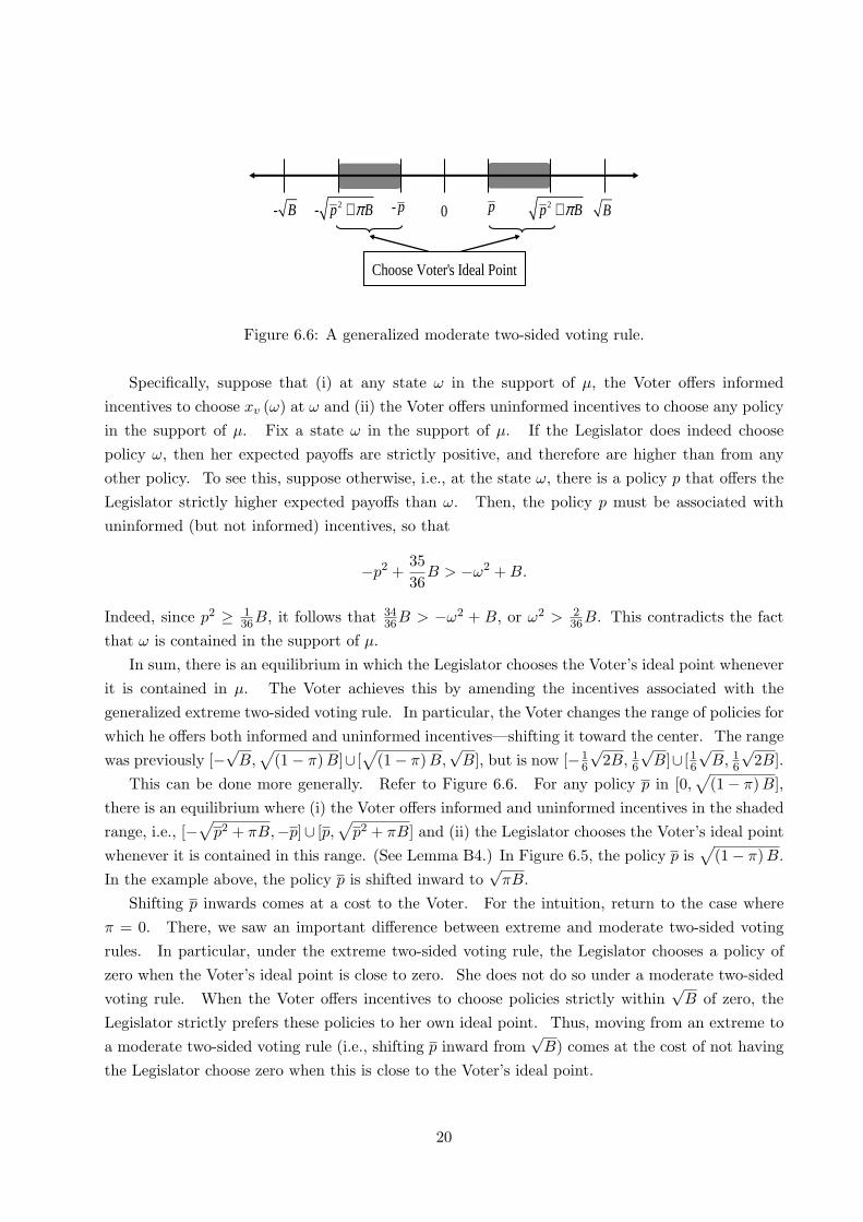
Figure 6.6: A generalized moderate two-sided voting rule.

Specifically, suppose that (i) at any state ω in the support of µ, the Voter offers informedincentives to choose xv (ω) at ω and (ii) the Voter offers uninformed incentives to choose any policyin the support of µ. Fix a state ω in the support of µ. If the Legislator does indeed choosepolicy ω, then her expected payoffs are strictly positive, and therefore are higher than from anyother policy. To see this, suppose otherwise, i.e., at the state ω, there is a policy p that offers theLegislator strictly higher expected payoffs than ω. Then, the policy p must be associated withuninformed (but not informed) incentives, so that

−p2 +3536

B > −ω2 + B.

Indeed, since p2 ≥ 136B, it follows that 34

36B > −ω2 + B, or ω2 > 236B. This contradicts the fact

that ω is contained in the support of µ.In sum, there is an equilibrium in which the Legislator chooses the Voter’s ideal point whenever

it is contained in µ. The Voter achieves this by amending the incentives associated with thegeneralized extreme two-sided voting rule. In particular, the Voter changes the range of policies forwhich he offers both informed and uninformed incentives—shifting it toward the center. The rangewas previously [−√B,

√(1− π) B]∪ [

√(1− π) B,

√B], but is now [−1

6

√2B, 1

6

√B]∪ [16

√B, 1

6

√2B].

This can be done more generally. Refer to Figure 6.6. For any policy p in [0,√

(1− π) B],there is an equilibrium where (i) the Voter offers informed and uninformed incentives in the shadedrange, i.e., [−

√p2 + πB,−p]∪ [p,

√p2 + πB] and (ii) the Legislator chooses the Voter’s ideal point

whenever it is contained in this range. (See Lemma B4.) In Figure 6.5, the policy p is√

(1− π) B.In the example above, the policy p is shifted inward to

√πB.

Shifting p inwards comes at a cost to the Voter. For the intuition, return to the case whereπ = 0. There, we saw an important difference between extreme and moderate two-sided votingrules. In particular, under the extreme two-sided voting rule, the Legislator chooses a policy ofzero when the Voter’s ideal point is close to zero. She does not do so under a moderate two-sidedvoting rule. When the Voter offers incentives to choose policies strictly within

√B of zero, the

Legislator strictly prefers these policies to her own ideal point. Thus, moving from an extreme toa moderate two-sided voting rule (i.e., shifting p inward from

√B) comes at the cost of not having

the Legislator choose zero when this is close to the Voter’s ideal point.

20

An analogous issue arises for generalized two-sided voting rules. Refer to the generalizedextreme two-sided voting rule associated with Figure 6.5. There, the Voter is able to use informedincentives alone to induce the Legislator to choose his ideal point when it is close to zero. As theVoter shifts p inward, the range in which these informed incentives are effective is reduced.

To see this, return to the example above. There p = 16

√B. Fix a state at which the Voter’s

ideal point ω is contained in (−16

√B, 1

6

√B) and suppose the Voter offers informed incentives to

choose the policy ω at this state.14 Then, the Legislator’s expected payoffs from choosing theVoter’s ideal point are −ω2 + 1

36B, while her expected payoffs from choosing the policy p = 16

√B

are 3436B. So, the Legislator will not choose the Voter’s ideal point at this state.In Section 6.3, we argued that we can combine the incentives associated with Figures 6.2 and

6.3, i.e., they do not conflict with one another. Here, we see that we may not be able to combinethe incentives associated with Figures 6.2 and 6.6. In particular, giving uninformed incentives forthe policy p (as in Figure 6.6) may conflict with using informed incentives to induce the Legislatorto choose a policy close to zero (as in Figure 6.2).

Fix a state ω. For these incentives not to conflict with one another, the Legislator’s expectedpayoffs from choosing p must be less than her expected payoffs from choosing the Voter’s idealpoint at this state. That is,

−xv (ω)2 + πB ≥ −p2 + (1− π) B.

There is some state that satisfies this condition if and only if p2 ≥ (1− 2π) B.

Proposition 6.2 Suppose that it is transparent that the Voter will be informed with some proba-bility strictly less than 1

2 , i.e., π ∈ [0, 12). Any State-by-State Optimal Equilibrium takes one of two

forms:

(i) There is a policy p ∈ [0,√

(1− 2π) B) such that the Legislator chooses the Voter’s ideal pointif and only if it is contained in [−

√p2 + πB,−p] ∪ [p,

√p2 + πB].

(ii) There are policies p ∈ [√

(1− 2π) B,√

(1− π)B] and q ∈ [0, p) such that the Legislatorchooses the Voter’s ideal point if and only if it is contained in [−

√p2 + πB,−p] ∪ [−q, q] ∪

[p,√

p2 + πB].

Proposition 6.2 says that, when π is strictly less than a half, an optimal retrospective votingrule must take one of three forms. The first form is a generalized version of a moderate two-sidedvoting rule. The second and form is a generalized version of an extreme two-sided voting rule.

In each of these cases, there is an open set of policies X such that the Legislator chooses theVoter’s true ideal point when it is contained in X. But, again, there is no Bayesian Equilibriumin which the Legislator chooses the Voter’s ideal point whenever it is contained in [−√B,

√B].

14This state is not in the support of the Voter’s prior. The example can be readily amended to include this statein the support (and retain the properties we discuss).

21

7 Enriching the Strategy Set: Behavioral Strategies

Thus far, we have restricted attention to pure-strategy Bayesian Equilibria. In this Section, weenrich the Voter’s strategy set by allowing him to use behavioral strategies. (The restriction tobehavioral, rather than mixed, strategies is without loss of generality.)

When it is transparent that Nature will inform the Voter with probability π ≥ 12 , allowing the

Voter this broader choice has no effect. In particular, as seen in Section 6.4, there exists a pure-strategy equilibrium in which the Legislator chooses the Voter’s ideal point whenever it is containedwithin

√B of zero. Even with the use of behavioral strategies, there do not exist incentives that

can induce the Legislator to choose the Voter’s ideal point when it is further than√

B from zero.So, the voting rule identified remains Expectationally and State-by-State Optimal, even within thislarger set of equilibria.

Turn to the case where it is transparent that Nature informs the Voter with probability π < 12 .

Now, allowing the Voter to play behavioral strategies does have an effect.15

Proposition 7.1 For all π ∈ [0, 1], there exists a Bayesian equilibrium in behavioral strategies, inwhich the Legislator chooses:

(i) the Voter’s ideal point, whenever it is contained within√

B of zero,

(ii) the policy −√B, whenever the Voter’s ideal point is less than −√B, and

(iii) the policy√

B, whenever the Voter’s ideal point is greater than√

B.

To understand this result, it will be useful to begin by assuming that the Voter is restricted tothe use of pure strategies and that π ∈ [0, 1

2). Recall that the Voter cannot induce the Legislator tochoose his ideal point both when his ideal point is a policy p ∈ (

√πB,

√(1− π) B) and when his

ideal point is√

B. To induce the Legislator to choose policy p, he must offer uninformed incentives.With these incentives, at any state, the Legislator’s expected payoffs are strictly greater than zero.But then, when the Voter’s true ideal point is

√B, the Legislator’s expected payoffs from choosing

p are strictly greater than zero, while her expected payoffs from choosing√

B are at most zero.Thus, she would not choose

√B at this state.

With the use of behavioral strategies, such a conflict need not occur. The Voter can offer theLegislator uninformed incentives with some probability less than one. In particular, the electoralrule can have the following features: at any state, if the policy p is chosen and the Voter isinformed, he reelects the Legislator with probability zero. If the policy p is chosen and the Voteris uninformed, he reelects the Legislator with probability p2

(1−π)B . Under this electoral rule, atevery state, the Legislator’s expected payoffs from choosing p are zero. Thus, in equilibrium, theLegislator can still choose

√B when this is the Voter’s ideal point.

This is again a result on full information extraction. In particular, it says that, when selectingamong the set of Bayesian equilibria in behavioral strategies, the optimal retrospective voting rule

15We thank Heski Bar-Isaac for suggesting this line of argument.

22

is ‘equivalent’ to the optimal retrospective voting rule when the Voter knows the true state of theworld. This is true even if it is transparent that the Voter has no chance of being informed, i.e.,if π = 0. The reason is that the Voter has a richer set of strategies and thus has gained ‘leverage.’

8 Discussion

This Section discusses some technical aspects and extensions of the paper.

8.1 The Players’ Payoff Functions

We assume that both players’ policy payoffs are quadratic. This assumption was made for tractabil-ity.

All of the results hold in a more general setting. Take the policy space to be a metrizable topo-logical space. We will require that there is a compatible metric that satisfies a certain ‘symmetry’property. (Lemma A9 suggests what that property must be.) For this metric, a player’s payoffmust be monotonically decreasing as policy moves away from his or her ideal point.

This is a key distinction between our paper and Maskin and Tirole [22, 2004]. In their game,there are only two actions and so the players’ preferences must violate the ‘symmetry’ propertywe require. As a result, their model does not yield the information extraction results on which wefocus.

8.2 Selection Criteria

In Section 4.2, we introduced two selection criteria, namely Expectational Optimality and State-by-State Optimality. The two concepts are distinct. The strategy profile (s∗l , s

∗v) may be a State-by-

State Optimal Equilibrium even though there does not exist a measure under which s∗l maximizesthe Voter’s expected payoffs given all Bayesian Equilibria.16 Conversely, the strategy profile (s∗l , s

∗v)

may be Expectationally Optimal even though it is not State-by-State Optimal. This can occur evenif we require the prior to have full support, i.e., if we can find a Bayesian Equilibrium (sl, sv) wherethe non-empty set

ω ∈ Ω : uv (ω, sl (ω)) > uv (ω, s∗l (ω))

does not contain a non-empty open subset.We note that there is a (conceptual) tension between Expectational Optimality and State-by-

State Optimality. The former requires that the Voter optimize given his prior µ. The latter is aweak dominance criterion—it asks the Voter to consider all possibilities, even though he may notbe able to do so under his prior µ.

That said, there is a rationale for including both requirements. Individually, each requirementcan be viewed as an ex ante optimality criterion. The Voter may be interested in using an interim

16This is for the same reason as the well-known fact: a strategy may be purely undominated even though it is nota best response under any probability measure.

23

optimality criterion, i.e., one where he would not want to revise his selection criterion at anyof his information sets. To the extent that Expectational Optimality is an appropriate ex anteselection criterion, it is an appropriate selection criterion at the information set where the Voteris uninformed. Now, consider an information set in which the Voter is informed that the truestate is ω. Here, the Voter would like to use a selection criterion that requires that there does notexist another Bayesian Equilibrium which yields a strictly higher expected payoff when the Voteris informed that the true state is ω. Collecting all these information sets together, the Voter wouldlike to use a weak dominance criterion—namely, State-by-State Optimality.

Many of the arguments in this paper depend only on State-by-State Optimality.17 To seethis, it will be useful to focus the discussion on the case where π = 0. The argument proceeds byconsidering a Bayesian Equilibrium, viz. (sl, sv), that differs structurally from a moderate or anextreme two-sided voting rule. For instance, suppose that sl is a constant strategy, i.e., specifies thesame policy at every state. We then argue that there is a two-sided Bayesian Equilibrium that (i)yields the Voter strictly higher payoffs for some non-empty set of states Φ and (ii) otherwise agreeswith the strategy sl. Thus, (sl, sv) is inconsistent with State-by-State Optimality. Note that, forthe strategy sl, the set Φ corresponds to an open set of ideal points. So, if xv is continuous andSuppµ = Ω, this also violates Expectational Optimality. But even if we were to assume that xv iscontinuous and µ has full-support, Expectational Optimality alone does not give the conclusionsof Proposition 5.2. Suppose that an extreme two-sided voting rule is Expectationally Optimal.We can find another Bayesian Equilibrium that differs from any extreme two-sided voting rule atexactly one state. Such an equilibrium will also be Expectationally Optimal, even though it is notState-by-State Optimal. As such, State-by-State Optimality is important for our analysis.

From the Voter’s perspective, the choice of an optimal voting rule is akin to finding an optimalmechanism (albeit from a limited set of mechanisms). Dominance has been important in otherareas of mechanism design (Vickery [28, 1961], Chung and Ely [9, 2001], Izmalkov [16, 2004]). Italso has a long history in voting games (Farquharson [12, 1969], Moulin [23, 1979], Dhillon andLockwood [11, 2004]).

8.3 The Legislator’s Policy Preferences

Thus far, we have analyzed the case where the Legislator’s policy preferences are independent ofthe state. In this subsection, we revisit the Benchmark specification, now allowing the Legislator’spolicy preferences to vary with the state.

Assume π = 0 and consider the follwoing example. If the Voter’s ideal point is contained inR\R+, the Legislator’s ideal point is p− ∈ [−√B, 0). Otherwise, the Legislator’s ideal point isp+ ∈ [0,

√B]. Consider any Bayesian Equilibrium in the Benchmark specification. We can find

a Bayesian Equilibrium of this new game that (up to a normalization) is equivalent to the initial17A notable exception is Lemma A13, which uses Expectational Optimality to pin down the policy p∗ associated

with a Moderate Two-Sided Voting Rule. Expectational Optimality is also important in selecting between a Moderateand an Extreme Two-Sided Voting Rule.

24


p q+ ++p q− −− p+p−0

Choose p q− −−

p q− −+ p q+ +−

Choose p q− −+ Choose p q+ +− Choose p q+ ++

Figure 8.1: The analogue to the Moderate Two-Sided Voting Rule with Two Partition Members.

equilibrium when we restrict (i) the Legislator’s ideal point to be negative (resp. positive) and (ii)the domain of the Voter’s strategy to be the set of negative (resp. positive) policies. The conversealso holds, i.e., for every Bayesian Equilibrium in the initial game, we can construct an equivalentBayesian Equilibrium in this new game.18

With this, the Voter can use a voting rule that is essentially one moderate two-sided voting ruleon the set of negative policies and another moderate two-sided voting rule on the set of positivepolicies.19 (See Figure 8.1.) Note that because the Legislator’s and Voter’s ideal points are alwayson the same side of zero, the Legislator never has an incentive to choose a policy in the ‘negativepartition member’ when the Voter would like her to choose a policy in the ‘positive partitionmember.’ So, if E (xv) ∈ [p−−√B, p+ +

√B], there is a Bayesian Equilibrium (sl, sv) where (i) at

every state, the Voter’s payoffs from sl are at least as high as are his payoffs from E (xv) and, (ii)at some states, the Voter’s payoffs from sl are strictly higher than his payoffs from E (xv).20

The basic set-up here suggests a first step toward generalization. In particular, let P be acountable partition of the policy space R. Each partition member, viz. Pk, is an interval of somelength less than or equal to 2

√B. The Legislator’s ideal point at state ω ∈ Ω will be determined

by the random variable xl : Ω → R where

xl (ω) = pk = sup Pk+inf Pk2 whenever xv (ω) ∈ Pk.

That is, whenever the Voter’s ideal point lies in the partition member Pk, the Legislator’s idealpoint is the policy pk, the midpoint of the partition member. Notice that this framework maintainsthe key assumption that the players’ ideal points always lie in the same partition member. Underthese assumptions, the Voter can again design a voting rule that he strictly prefers to the strategywhere he receives his expected ideal point at every state. (See the Online Appendix for a formaltreatment.)

If the Legislator’s policy preferences are associated with K partition members, in any equilib-18The statements in this paragraph hold even when p− +

√B < 0 or p+ −√B > 0.

19A similar argument can be made with respect to an Extreme Two-Sided Voting Rule, though the argument ismore intricate when p− +

√B > 0 or p+ −√B < 0. (See Footnote 18.)

20Note that the constant strategy associated with E (xv) may be inconsistent with any Bayesian Equilibrium.

25

rium, there are, at most, 2K policies for which the Voter offers electoral incentives that actuallyinduce the Legislator to choose such policies. As K increases, the Voter can offer more (effective)electoral incentives. So, if the players’ ideal points always lie in the same partition member, in-creasing K makes it easier for the Voter to extract information.21 However, increasing K has asecond effect. When the partition members are not required to be symmetric around the Legisla-tor’s ideal point, the incentives a Voter provides the Legislator within one partition member canconflict with the incentives provided in another partition member.22 Put differently, as K increases,the informational extraction problem becomes easier, while the discipline problem becomes moredifficult.

One goal of this paper was to provide an informational rationale for retrospective voting. Withthis in mind, we focused on the problem of extracting information. We restricted attention to thecase where the informational extraction problem is most difficult, i.e., K = 1. Of course, it isimportant to understand the ability of the Voter to extract information in the presence of theseconflicting incentives. It is also important to understand the Voter’s ability to extract information(under these conflicting incentives) when he can use a richer set of strategies. We leave thesecharacterizations for future work.

21In the extreme case, the players’ preferences are perfectly aligned, and the information extraction problem istrivial.

22This is why we made the above assumptions about xl. See the Online Appendix for more on these difficulties.

26

Appendix A: Proofs for Section 5

This Appendix provides the proofs for Section 5. As such, throughout this Appendix, we takethe notational conventions outlined at the beginning of that Section. We begin with the proof ofProposition 5.1. This will require a number of auxiliary results, found in Lemmata A1-A5.

Lemma A1 Fix a strategy sv ∈ Sv. Then there exists some sl ∈ Sl such that (sl, sv) ∈ Sl × Sv isa Bayesian Equilibrium if and only if there exists p ∈ R that maximizes ul (·, sv (·)).

Proof. Fix a strategy sv ∈ Sv. First, suppose that there exists p ∈ R that maximizes ul (·, sv (·)).Set sl : Ω → R so that sl (ω) = p for all ω ∈ Ω. It is immediate that sl is Borel measurable. For allω ∈ Ω,

ul (sl (ω) , sv (sl (ω))) ≥ ul (p, sv (p)) for all p ∈ R,

establishing that (sl, sv) is a Bayesian Equilibrium. Conversely, fix a Bayesian Equilibrium (sl, sv).By Condition (ii) of a Bayesian Equilibrium,

ul (sl (ω) , sv (sl (ω))) ≥ ul (p, sv (p)) for all p ∈ R,

holds for all ω ∈ Ω. So, for any given ω ∈ Ω, sl (ω) ∈ R maximizes ul (·, sv (·)), as required.It will be convenient to introduce a piece of notation. Let P be a binary, complete, and transitive

ordering relation on R × R such that 〈p, q〉 ∈ P if and only if p2 ≥ q2. Say q is a lower boundon X ⊆ R with respect to the order relation P if 〈p, q〉 ∈ P for all p ∈ X. Say q is the greatestpositive lower bound on X (with respect to the order relation P) if q is a greatest lower bound onX and q ≥ 0. (So, if X = (−2,−1) then there are two greatest lower bounds, viz. −1 and 1, andone greatest positive lower bound, 1.)

Fix some strategy sv ∈ Sv. Let inf (sv) be the greatest positive lower bound on the set ofpolicies (sv)

−1 (1) with respect to the order relation P. Notice that inf (sv) ≥ 0.

Lemma A2 Fix a strategy sv ∈ Sv where, for some p ∈ R, sv (p) = 1 and B ≥ p2. If sv(− inf (sv) ,

inf (sv)) = 0, then there does not exist a strategy sl ∈ Sl such that (sl, sv) ∈ Sl×Sv is a BayesianEquilibrium.

Proof. Fix a strategy sv ∈ Sv that satisfies the conditions in the statement of the Lemma. Noticethat there exists a policy p ∈ R with sv (p) = 1 and B > p2. To see this, suppose otherwise: usingthe statement of the Lemma, there exists some p ∈ R with sv (p) = 1 and B = p2. Moreover, forall p ∈ R with p2 > p2, sv (p) = 0. So, inf (sv) = |p| contradicting sv (− inf (sv)) = sv (inf (sv)) = 0.

Assume, contra hypothesis, that there exists a strategy sl ∈ Sl where (sl, sv) is a Bayesianequilibrium. Fix some ω ∈ Ω and the policy it induces under sl, viz sl (ω). There will be two cases,the first corresponding to sv (sl (ω)) = 1 and the second corresponding to sv (sl (ω)) = 0.

Case A (sv (sl (ω)) = 1): Since sv (− inf (sv)) = sv (inf (sv)) = 0 and sv (sl (ω)) = 1, itfollows that sl (ω)2 > inf (sv)

2. From this, we know that there must exist some policy p ∈ R with

27

[sl (ω)]2 > p2 > [inf (sv)]2 and sv (p) = 1, else [sl (ω)]2 = [inf (sv)]

2. Now

ul (p, sv (p)) = −p2 + B

> − [sl (ω)]2 + B = ul (sl (ω) , sv (sl (ω))) ,

contradicting Condition (ii) of a Bayesian Equilibrium.Case B (sv (sl (ω)) = 0): Here

ul (p, sv (p)) = −p2 + B

> −B + B ≥ − [sl (ω)]2 ≥ ul (sl (ω) , sv (sl (ω))) ,

contradicting Condition (ii) of a Bayesian Equilibrium.

Lemma A3 Fix a Bayesian Equilibrium (sl, sv) ∈ Sl × Sv. Suppose that either (i) sv (0) = 1 or(ii) for any p ∈ R with sv (p) = 1, p2 > B. Then sl (Ω) = 0.

Proof. First suppose Condition (i) is satisfied. Then

ul (0, sv (0)) = B > −p2 + B ≥ ul (p, sv (p)) ,

for all p ∈ R\ 0. By Condition (ii) of a Bayesian Equilibrium, there cannot exist some ω ∈ Ωwith sl (ω) ∈ R\ 0.

Next, suppose that Condition (ii) is satisfied. Fix some p ∈ R\ 0. If sv (p) = 1 then p2 > B

so that

ul (0, sv (0)) ≥ −B + B

> −p2 + B = ul (p, sv (p)) .

If sv (p) = 0 thenul (0, sv (0)) ≥ 0 > −p2 = ul (p, sv (p)) .

Again, using Condition (ii) of a Bayesian Equilibrium, there cannot exist some ω ∈ Ω with sl (ω) ∈R\ 0.

Lemma A4 Fix a Bayesian Equilibrium (sl, sv) ∈ Sl × Sv with B > inf (sv)2. Then sl (Ω) ⊆

− inf (sv) , inf (sv) and, for all ω ∈ Ω, sv (sl (ω)) = 1.

Proof. Fix a Bayesian Equilibrium (sl, sv). By Lemma A2 and the fact that B > inf (sv)2,

either sv (− inf (sv)) = 1 or sv (inf (sv)) = 1. First, we will show that, for any ω ∈ Ω, sl (ω) ∈− inf (sv) , inf (sv). For the purposes of this argument, suppose that sv (− inf (sv)) = 1. (Acorresponding argument will work if sv (inf (sv)) = 1.) Fix p ∈ R\ − inf (sv) , inf (sv). If sv (p) =

28

1 then p2 > [inf (sv)]2, so that

ul (− inf (sv) , sv (− inf (sv))) = − [inf (sv)]2 + B

> −p2 + B ≥ ul (p, sv (p)) .

If sv (p) = 0 then

ul (− inf (sv) , sv (− inf (sv))) = − [inf (sv)]2 + B

> −B + B ≥ ul (p, sv (p)) .

So, by Condition (ii) of a Bayesian Equilibrium, sl (ω) ∈ − inf (sv) , inf (sv), for any ω ∈ Ω.Next suppose that, for some ω ∈ Ω, sv (sl (ω)) = 0. Since sl (ω) ∈ − inf (sv) , inf (sv) and

sv (− inf (sv) , inf (sv)) 6= 0, sv (−sl (ω)) = 1. From this it follows

ul (−sl (ω) , sv (−sl (ω))) = − [sl (ω)]2 + B

> − [sl (ω)]2 = ul (sl (ω) , sv (sl (ω))) ,


Lemma A5 Fix a Bayesian Equilibrium (sl, sv) ∈ Sl × Sv with B = inf (sv)2. Then sl (Ω) ⊆

0,−√B,√

B, and sv (sl (ω)) = 1 if sl (ω) ∈ −√B,√

B.

Proof. Fix a Bayesian Equilibrium (sl, sv). First, we will show that, for each ω ∈ Ω, sl (ω) is notcontained in R\ 0,− inf (sv) , inf (sv). Then, we will show that, if sl (ω) ∈ − inf (sv) , inf (sv)then sv (sl (ω)) = 1.

Fix some policy p ∈ R\ 0,− inf (sv) , inf (sv). If sv (p) = 1 then p2 > B, and so

ul (0, sv (0)) = −B + B

> −p2 + B = ul (p, sv (p)) .

Similarly, if sv (p) = 0 thenul (0, sv (0)) > −p2 = ul (p, sv (p)) .

¿From this and Condition (ii) of a Bayesian Equilibrium, for all ω ∈ Ω, sl (ω) ∈ 0,− inf (sv) , inf (sv).Next, suppose that sl (ω) ∈ − inf (sv) , inf (sv) and sv (sl (ω)) = 0. Then

ul (0, sv (0)) > −B = ul (sl (ω) , sv (sl (ω))) ,

contradicting Condition (ii) of a Bayesian Equilibrium. This establishes that if sl (ω) ∈ − inf (sv) , inf (sv)then sv (sl (ω)) = 1, as required.Proof of Proposition 5.1. Immediate from Lemmata A2-A3-A4-A5.

29

Next, we turn to the verbal claim that, if the Voter could choose his own policy, then maximizinghis expected utility would require that he always choose his expected ideal point. We formalize thisclaim as follows: suppose that the Voter could choose a strategy sl for the Legislator. Unlike theLegislator’s choice, the Voter’s choice cannot be state-contingent because he does not know the truestate. That is, the Voter can only choose a constant strategy, i.e., a strategy sl with sl (ω) = sl (ω′)for all ω, ω′ ∈ Ω. With this, it suffices to show the following:

Lemma A6 Let E (xv) =∫Ω xv (ω) dµ (ω) and let sl : Ω → R be a constant strategy with sl (Ω) =

E (xv). Then, for any constant strategy rl : Ω → R,

∫

Ωuv (ω, sl (ω)) dµ (ω) ≥

∫

Ωuv (ω, rl (ω)) dµ (ω) .

Proof. Fix a constant strategy rl : Ω → R with rl (Ω) = p. Note

∫

Ωuv (ω, rl (ω)) dµ (ω) = −

∫

Ωrl (ω)2 dµ (ω) + 2

∫

Ωrl (ω) xv (ω) dµ (ω)−

∫

Ωxv (ω)2 dµ (ω)

= −p2 + 2pE (xv)−E (xv)2 + E (xv)

2 −∫

Ωxv (ω)2 dµ (ω)

= − (p−E (xv))2 − var (xv) ,

where var (xv) denotes the variance of the random variable xv with respect to µ. Applying this tosl and an arbitrary constant strategy rl,

∫

Ωuv (ω, sl (ω)) dµ (ω) = − var (xv)

≥ − (rl (ω)− E (xv))2 − var (xv) =

∫

Ωuv (ω, rl (ω)) dµ (ω) ,

as required.We now turn to the proof of Proposition 5.2, which begins with what is known from Proposition

5.1 and then proceeds ‘to rule out’ certain Bayesian Equilibria based on the criteria of Expectational(Lemma A13) and State-by-State Optimality (A9, A11, and A15). We also establish that Moderateand Extreme Two-Sided Voting Rules are indeed State-by-State Optimal Equilibria, and at leastone is Expectationally Optimal. Again, this will require a number of auxiliary results, found below.

Lemma A7 Let P1, P2, .. be a countable partition of R where each partition member Pk is mea-surable. Also fix some countable p1, p2, .. ⊆ R. Fix a strategy sl ∈ Sl with sl (ω) = pk wheneverxv (ω) ∈ Pk. Then sl is measurable.

Proof. Fix some measurable set X ⊆ R. Write Xk = X ∩ Pk and note that it is measurable sincePk is measurable. It suffices to show that each set (sl)

−1 (Xk) is measurable; if so, (sl)−1 (X) is

a countable union of measurable sets and so measurable. If pk /∈ Xk then (sl)−1 (Xk) = ∅ and so

measurable. If pk ∈ Xk then (sl)−1 (Xk) = (xv)

−1 (Xk). Since xv is measurable, (xv)−1 (Xk) is a

measurable set, as required.

30

Lemma A8 Fix (sl, sv) ∈ Sl × Sv satisfying the following properties. The strategy sl ∈ Sl has (i)sl (ω) = 0 if xv (ω) ∈ [−1

2

√B, 1

2

√B], (ii) sl (ω) = −√B if −1

2

√B > xv (ω), and (iii) sl (ω) =

√B

if xv (ω) > 12

√B. For all p ∈ [−√B,

√B], sv (p) = 1 if and only if p ∈ −√B,

√B. Then (sl, sv)

is a Bayesian Equilibrium.

Proof. Condition (i) (of a Bayesian Equilibrium) follows from Lemma A7. Next, fix some ω ∈ Ω.If sl (ω) = 0, ul (sl (ω) , sv (sl (ω))) = 0. If sl (ω) 6= 0, then ul (sl (ω) , sv (sl (ω))) = −B + B = 0.For any p ∈ R\0,−√B,

√B, 0 > −p2 = ul (p, sv (p)). This establishes Condition (ii).

Remark A1 The strategy profile (sl, sv) ∈ Sl × Sv in the statement of Lemma A8 is an ExtremeTwo-Sided Voting Rule. An argument analogous to the proof of Lemma A8 establishes that anyExtreme Two-Sided Voting Rule is a Bayesian Equilibrium.

Recall from the text that Ω+ = ω ∈ Ω : xv (ω) ≥ 0.

Lemma A9 Fix a Bayesian Equilibrium (rl, rv) ∈ Sl × Sv where rl is a constant strategy. Thenthere is a Bayesian Equilibrium (sl, sv) ∈ Sl × Sv and a non-empty set of states Φ ⊆ Ω with

uv (ω, sl (ω)) ≥ uv (ω, rl (ω)) for all ω ∈ Ωuv (ω, sl (ω)) > uv (ω, rl (ω)) for all ω ∈ Φ.

Proof. Fix a Bayesian Equilibrium (rl, rv) where rl is a constant strategy. We will assume that, forall ω ∈ Ω, rl (ω) = p ≥ 0. (A corresponding argument will work when p ≤ 0.) It will be convenientto break up the proof into two cases. The first corresponds to p > 0. The second corresponds top = 0.

Case A (p > 0): First notice that rv (p) = 1. If not,

ul (0, rv (0)) > −p2 = ul (p, rv (p)) ,

contradicting Condition (ii) of a Bayesian Equilibrium. Also note that B ≥ p2. If not,

ul (0, rv (0)) ≥ −B + B

> −p2 + B = ul (p, rv (p)) ,

contradicting Condition (ii) of a Bayesian Equilibrium. Construct (sl, sv) as follows. Let

sl (ω) =

−p if ω ∈ Ω\Ω+

p if ω ∈ Ω+,

and let sv (p) = 1 if and only if p ∈ −p, p. By Lemma A7, sl is measurable. Also notice that, forany ω ∈ Ω,

ul (sl (ω) , sv (sl (ω))) = −p2 + B ≥ 0,

31

since B > p2. For any p ∈ R,

ul (p, sv (p)) =

−p2 + B if p ∈ −p, p−p2 otherwise

.

Put together, this establishes Condition (ii) of a Bayesian Equilibrium. As such, (sl, sv) is aBayesian Equilibrium.

Now note that, for any ω ∈ Ω\Ω+, we have

uv (ω, sl (ω)) = −[p2 + 2pxv (ω) + xv (ω)2

]

> −[p2 − 2pxv (ω) + xv (ω)2

]= uv (ω, rl (ω)) .

Take Φ = Ω\Ω+ and note Φ is non-empty since xv is surjective. Now note that, for ω ∈ Ω+,sl (ω) = rl (ω) and so uv (ω, sl (ω)) = uv (ω, rl (ω)), as required.

Case B (p = 0): Choose (sl, sv) to be a Bayesian Equilibrium, as in the statement of LemmaA8. When xv (ω) ∈ [−1

2

√B, 1

2

√B], sl (ω) = rl (ω) and so uv (ω, sl (ω)) = uv (ω, rl (ω)). Next,

suppose that −12

√B > xv (ω). Here,

uv (ω, sl (ω)) = −[B + 2

√Bxv (ω) + xv (ω)2

]

> − [xv (ω)]2 = uv (ω, rl (ω)) ,

where the second line follows from the fact that −12

√B > xv (ω) and so 0 > B + 2

√Bxv (ω).

Similarly, for xv (ω) > 12

√B,

uv (ω, sl (ω)) = −[B − 2

√Bxv (ω) + xv (ω)2

]

> − [xv (ω)]2 = uv (ω, rl (ω)) ,

where the second line uses the fact that xv (ω) > 12

√B and so 0 > B − 2

√Bxv (ω). Take Φ =

ω ∈ Ω : xv (ω) /∈ [−12

√B, 1

2

√B]

. Since xv is surjective, Φ is non-empty.

Lemma A10 Fix p ∈ (0,√

B) and construct (sl, sv) ∈ Sl × Sv as follows: Let sl (ω) = −p ifω ∈ Ω\Ω+, sl (ω) = p if ω ∈ Ω+\ (xv)

−1 (0), and sl (ω) ∈ −p, p otherwise. For all p ∈ [−p, p],sv (p) = 1 if and only if p ∈ −p, p. Then (sl, sv) is a Bayesian Equilibrium.

Proof. Lemma A7 establishes that sl is measurable. To establish Condition (ii) of a BayesianEquilibrium, fix some ω ∈ Ω. If p ∈ (−p, p), then

ul (sl (ω) , sv (sl (ω))) = −p2 + B

> −B + B

≥ −p2 = ul (p, sv (p)) .

32

If p /∈ (−p, p), then p2 ≥ p2 so that

ul (sl (ω) , sv (sl (ω))) = −p2 + B

≥ −p2 + B ≥ ul (p, sv (p)) ,

as required.

Remark A2 Any Moderate Two-Sided Voting Rule satisfies the conditions of Lemma A10.


B) and some associated strategy profile, viz. (sl, sv) ∈ Sl × Sv, as inthe statement of Lemma A10. Let (rl, rv) ∈ Sl×Sv be a Bayesian Equilibrium where rv (p) = sv (p)for all p ∈ [−p, p]. Then

uv (ω, sl (ω)) ≥ uv (ω, rl (ω)) for all ω ∈ Ω.

Moreover, there exists some non-empty set of states Φ ⊆ Ω with

uv (ω, sl (ω)) > uv (ω, rl (ω)) for all ω ∈ Φ

if and only if there exists some ω ∈ (xv)−1 (R\ 0) with rl (ω) 6= sl (ω).

Proof. Fix some p ∈ (0,√

B). Also fix (sl, sv) and (rl, rv) as in the statement of the Lemma. Take

Φ = (xv)−1 (R\ 0) ∩ ω ∈ Ω : rl (ω) 6= sl (ω) .

We need to show that (i) for any ω ∈ Ω, uv (ω, sl (ω)) ≥ uv (ω, rl (ω)), and (ii) ω ∈ Ω if and onlyif uv (ω, sl (ω)) > uv (ω, rl (ω)). To do so, we will break the proof into two parts. First, we willshow that if ω ∈ Φ, then uv (ω, sl (ω)) > uv (ω, rl (ω)). Second, we will show that if ω ∈ Ω\Φ, thenuv (ω, sl (ω)) = uv (ω, rl (ω)).

In showing these facts, it is useful to note that rl (Ω) ⊆ −p, p. This follows from the fact that(rl, rv) is a Bayesian Equilibrium and Lemma A4.

Begin with some ω ∈ Φ. If ω ∈ Ω\Ω+, then rl (ω) = p. Use the fact that 0 > xv (ω) to get

uv (ω, sl (ω)) = −[p2 + 2pxv (ω) + xv (ω)2

]

> −[p2 − 2pxv (ω) + xv (ω)2

]= uv (ω, rl (ω)) .

Also, if ω ∈ Ω+\ (xv)−1 (0), then rl (ω) = −p. Now, xv (ω) > 0 implies

uv (ω, sl (ω)) = −[p2 − 2pxv (ω) + xv (ω)2

]

> −[p2 + 2pxv (ω) + xv (ω)2

]= uv (ω, rl (ω)) .

33

Taken together, these displays establish that if ω ∈ Φ, then uv (ω, sl (ω)) > uv (ω, rl (ω)). Next, fixω ∈ Ω\Φ. Either xv (ω) = 0 or sl (ω) = rl (ω). If the former,

uv (ω, sl (ω)) = −p2 = uv (ω, rl (ω)) .

If the latter, it is immediate that uv (ω, sl (ω)) = uv (ω, rl (ω)).


B) and some associated strategy profile, viz. (sl, sv) ∈ Sl × Sv, as inthe statement of Lemma A10. Then (sl, sv) is State-by-State Optimal.

Proof. Fix a Bayesian Equilibrium (rl, rv) ∈ Sl × Sv. We will show that either (i) for all ω ∈ Ω,uv (ω, sl (ω)) = uv (ω, rl (ω)) or (ii) there exists ω ∈ Ω with uv (ω, sl (ω)) > uv (ω, rl (ω)).

Proposition 5.1 tells us that, there exists some q ∈ [0,√

B] such that rl (Ω) ⊆ 0,−q, q. Wewill make use of this fact below.

Case A: Here q 6= p. Fix some ω ∈ Ω with xv (ω) = p. (Since xv is surjective, such a stateexists.) Then

uv (ω, sl (ω)) = 0 > − (rl (ω)− p)2 = uv (ω, rl (ω)) ,

as required.Case B: Here q = p. Proposition 5.1 tells us that rl (Ω) ⊆ −p, p. If sl (Ω) = rl (Ω) then

certainly we have (i). So suppose there is a state ω ∈ Ω with sl (ω) 6= rl (ω). If the state ω iscontained in Ω\Ω+ then 0 > xv (ω) and rl (ω) = p. It follows that

uv (ω, sl (ω)) = −[p2 + 2pxv (ω) + xv (ω)2

]

> −[p2 − 2pxv (ω) + xv (ω)2

]= uv (ω, rl (ω)) ,

as required. An analogous argument works when the state ω is contained in Ω+\ (xv)−1 (0).

Since xv (ω) > 0 and rl (ω) = −p,

uv (ω, sl (ω)) = −[p2 − 2pxv (ω) + xv (ω)2

]

> −[p2 + 2pxv (ω) + xv (ω)2

]= uv (ω, rl (ω)) ,

as required. Finally, if ω ∈ (xv)−1 (0) then certainly uv (ω, sl (ω)) = uv (ω, rl (ω)).

Lemma A13 Define

p =∫

Ω+


Ω\Ω+

xv (ω) dµ (ω) .

Fix a strategy sl ∈ Sl where sl (ω) = −p if ω ∈ Ω\Ω+, sl (ω) = p if ω ∈ Ω+\ (xv)−1 (0), and

sl (ω) ∈ −p, p otherwise. Let rl ∈ Sl be a strategy where, for some p ≥ 0, rl (ω) = −p ifω ∈ Ω\Ω+, rl (ω) = p if ω ∈ Ω+\ (xv)

−1 (0), and rl (ω) ∈ −p, p otherwise. Then

∫

Ωuv (ω, sl (ω)) dµ (ω) ≥

∫

Ωuv (ω, rl (ω)) dµ (ω) .

34

Proof. Note that∫

Ωuv (ω, rl (ω)) dµ (ω) = −

∫

Ω+

(p− xv (ω))2 dµ (ω)−∫

Ω\Ω+

(−p− xv (ω))2 dµ (ω)

= −∫

Ω+

[p2 − 2pxv (ω) + xv (ω)2

]dµ (ω)−

∫

Ω\Ω+

[p2 + 2pxv (ω) + xv (ω)2

]dµ (ω)

= −p2 + 2p

[∫

Ω+


Ω\Ω+

xv (ω) dµ (ω)

]−

∫

Ωxv (ω)2 dµ (ω) .

Choosing p ∈ R to maximize∫Ω uv (ω, rl (ω)) dµ (ω) requires

p =∫

Ω+


Ω\Ω+

xv (ω) dµ (ω) .

(The second derivative of∫Ω uv (ω, rl (ω)) dµ (ω) is −2, so that this is indeed a maximum.)

Lemma A14 Suppose that

p =∫

Ω+


Ω\Ω+

xv (ω) dµ (ω) .

Fix a strategy sl ∈ Sl (viz. rl ∈ Sl) where sl (ω) = −p (resp. rl (ω) = −q) if ω ∈ Ω\Ω+, sl (ω) = p

(resp. rl (ω) = q) if ω ∈ Ω+\ (xv)−1 (0), and sl (ω) ∈ −p, p (resp. rl (ω) ∈ −q, q) otherwise.

If p > p > q, then ∫uv (ω, sl (ω)) dµ (ω) ≥

∫uv (ω, rl (ω)) dµ (ω) .

Proof. This follows from the proof of Lemma A13: Note that

d

dp

[∫

Ω+

uv (ω, rl (ω)) dµ(ω)]

= 2

[∫

Ω+


Ω\Ω+

xv (ω) dµ (ω)

]− 2p

is strictly positive whenever

[∫

Ω+


Ω\Ω+

xv (ω) dµ (ω)

]> p,

as required.

Lemma A15 Let (sl, sv) ∈ Sl×Sv be as in the statement of Lemma A8. Suppose (rl, rv) ∈ Sl×Sv

is a Bayesian Equilibrium where rv (p) = sv (p) for all p ∈ [−√B,√

B]. Then

uv (ω, sl (ω)) ≥ uv (ω, rl (ω)) for all ω ∈ Ω.

Moreover, there exists a non-empty set of states Φ ⊆ Ω with

uv (ω, sl (ω)) > uv (ω, rl (ω)) for all ω ∈ Φ

35

if and only if there exists ω ∈ Ω satisfying one of the following properties:

A. xv (ω) /∈ −12

√B, 1

2

√B and rl (ω) 6= sl (ω);

B. xv (ω) = −12

√B and rl (ω) =

√B;

C. xv (ω) = 12

√B and rl (ω) = −√B.

Proof. Fix a Bayesian Equilibrium (rl, rv). By Lemma A5, rl (Ω) ⊆ 0,−√B,√

B. We willshow that (i) for all ω ∈ Ω, uv (ω, sl (ω)) ≥ uv (ω, rl (ω)) and (ii) there exists some ω ∈ Ω withuv (ω, sl (ω)) > uv (ω, rl (ω)) if and only if there exists some ω ∈ Ω satisfying any one of ConditionsA, B, or C in the statement of the Lemma.

To do so, we will take

ΦA =

ω ∈ Ω : xv (ω) /∈−1

2

√B,

12

√B

and rl (ω) 6= sl (ω)

ΦB =

ω ∈ Ω : xv (ω) = −12

√B and rl (ω) =

√B

ΦC =

ω ∈ Ω : xv (ω) =12

√B and rl (ω) = −

√B

.

First, we will show that if ω ∈ ΦA ∪ ΦB ∪ ΦC , then uv (ω, sl (ω)) > uv (ω, rl (ω)). Second, we willshow that if ω ∈ Ω\ (ΦA ∪ ΦB ∪ ΦC), then uv (ω, sl (ω)) = uv (ω, rl (ω)).

Case 1A: Fix some ω ∈ ΦA. Here, xv (ω) ∈ (−12

√B, 1

2

√B) if and only if rl (ω) ∈ −√B,

√B.

If rl (ω) = −√B,

uv (ω, sl (ω)) = − [xv (ω)]2

> −[B + 2

√Bxv (ω) + xv (ω)2

]= uv (ω, rl (ω)) ,

where the inequality follows from the fact that xv (ω) > −12

√B and so B + 2

√Bxv (ω) > 0. If

rl (ω) =√

B,

uv (ω, sl (ω)) = − [xv (ω)]2

> −[B − 2

√Bxv (ω) + xv (ω)2

]= uv (ω, rl (ω)) ,

where the inequality follows from the fact that 12

√B > xv (ω) and so B − 2

√Bxv (ω) > 0. Next,

notice that −12

√B > xv (ω) if and only if rl (ω) ∈ 0,

√B. If rl (ω) = 0,

uv (ω, sl (ω)) = −[B + 2

√Bxv (ω) + xv (ω)2

]

> − [xv (ω)]2 = uv (ω, rl (ω)) ,

36

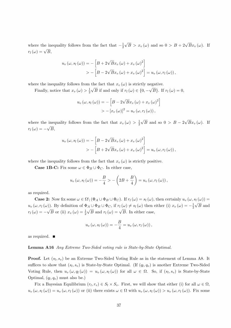
where the inequality follows from the fact that −12

√B > xv (ω) and so 0 > B + 2

√Bxv (ω). If

rl (ω) =√

B,

uv (ω, sl (ω)) = −[B + 2

√Bxv (ω) + xv (ω)2

]

> −[B − 2

√Bxv (ω) + xv (ω)2

]= uv (ω, rl (ω)) ,

where the inequality follows from the fact that xv (ω) is strictly negative.Finally, notice that xv (ω) > 1

2

√B if and only if rl (ω) ∈ 0,−√B. If rl (ω) = 0,

uv (ω, sl (ω)) = −[B − 2

√Bxv (ω) + xv (ω)2

]

> − [xv (ω)]2 = uv (ω, rl (ω)) ,

where the inequality follows from the fact that xv (ω) > 12

√B and so 0 > B − 2

√Bxv (ω). If

rl (ω) = −√B,

uv (ω, sl (ω)) = −[B − 2

√Bxv (ω) + xv (ω)2

]

> −[B + 2

√Bxv (ω) + xv (ω)2

]= uv (ω, rl (ω)) ,

where the inequality follows from the fact that xv (ω) is strictly positive.Case 1B-C: Fix some ω ∈ ΦB ∪ ΦC . In either case,

uv (ω, sl (ω)) = −B

4> −

(2B +

B

4

)= uv (ω, rl (ω)) ,

as required.Case 2: Now fix some ω ∈ Ω\ (ΦA ∪ ΦB ∪ ΦC). If rl (ω) = sl (ω), then certainly uv (ω, sl (ω)) =

uv (ω, rl (ω)). By definition of ΦA ∪ ΦB ∪ ΦC , if rl (ω) 6= sl (ω) then either (i) xv (ω) = −12

√B and

rl (ω) = −√B or (ii) xv (ω) = 12

√B and rl (ω) =

√B. In either case,

uv (ω, sl (ω)) = −B

4= uv (ω, rl (ω)) ,

as required.

Lemma A16 Any Extreme Two-Sided voting rule is State-by-State Optimal.

Proof. Let (sl, sv) be an Extreme Two-Sided Voting Rule as in the statement of Lemma A8. Itsuffices to show that (sl, sv) is State-by-State Optimal. (If (ql, qv) is another Extreme Two-SidedVoting Rule, then uv (ω, ql (ω)) = uv (ω, sl (ω)) for all ω ∈ Ω. So, if (sl, sv) is State-by-StateOptimal, (ql, qv) must also be.)

Fix a Bayesian Equilibrium (rl, rv) ∈ Sl × Sv. First, we will show that either (i) for all ω ∈ Ω,uv (ω, sl (ω)) = uv (ω, rl (ω)) or (ii) there exists ω ∈ Ω with uv (ω, sl (ω)) > uv (ω, rl (ω)). Fix some

37

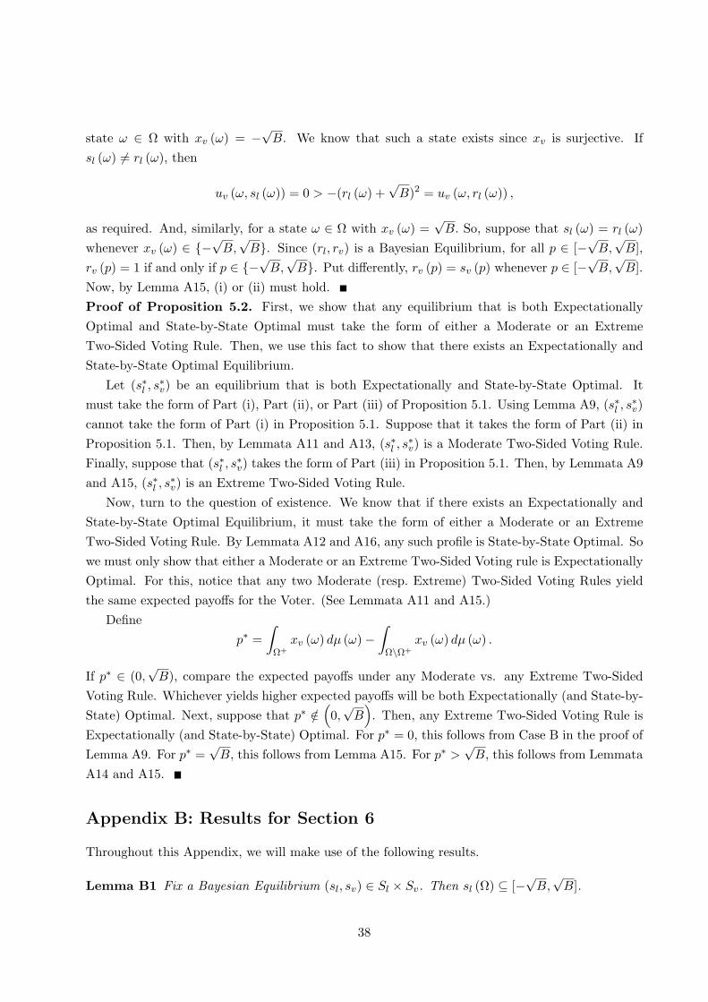
state ω ∈ Ω with xv (ω) = −√B. We know that such a state exists since xv is surjective. Ifsl (ω) 6= rl (ω), then

uv (ω, sl (ω)) = 0 > −(rl (ω) +√

B)2 = uv (ω, rl (ω)) ,

as required. And, similarly, for a state ω ∈ Ω with xv (ω) =√

B. So, suppose that sl (ω) = rl (ω)whenever xv (ω) ∈ −√B,

√B. Since (rl, rv) is a Bayesian Equilibrium, for all p ∈ [−√B,

√B],

rv (p) = 1 if and only if p ∈ −√B,√

B. Put differently, rv (p) = sv (p) whenever p ∈ [−√B,√

B].Now, by Lemma A15, (i) or (ii) must hold.Proof of Proposition 5.2. First, we show that any equilibrium that is both ExpectationallyOptimal and State-by-State Optimal must take the form of either a Moderate or an ExtremeTwo-Sided Voting Rule. Then, we use this fact to show that there exists an Expectationally andState-by-State Optimal Equilibrium.

Let (s∗l , s∗v) be an equilibrium that is both Expectationally and State-by-State Optimal. It

must take the form of Part (i), Part (ii), or Part (iii) of Proposition 5.1. Using Lemma A9, (s∗l , s∗v)

cannot take the form of Part (i) in Proposition 5.1. Suppose that it takes the form of Part (ii) inProposition 5.1. Then, by Lemmata A11 and A13, (s∗l , s

∗v) is a Moderate Two-Sided Voting Rule.

Finally, suppose that (s∗l , s∗v) takes the form of Part (iii) in Proposition 5.1. Then, by Lemmata A9

and A15, (s∗l , s∗v) is an Extreme Two-Sided Voting Rule.

Now, turn to the question of existence. We know that if there exists an Expectationally andState-by-State Optimal Equilibrium, it must take the form of either a Moderate or an ExtremeTwo-Sided Voting Rule. By Lemmata A12 and A16, any such profile is State-by-State Optimal. Sowe must only show that either a Moderate or an Extreme Two-Sided Voting rule is ExpectationallyOptimal. For this, notice that any two Moderate (resp. Extreme) Two-Sided Voting Rules yieldthe same expected payoffs for the Voter. (See Lemmata A11 and A15.)

Definep∗ =

∫

Ω+


Ω\Ω+

xv (ω) dµ (ω) .

If p∗ ∈ (0,√

B), compare the expected payoffs under any Moderate vs. any Extreme Two-SidedVoting Rule. Whichever yields higher expected payoffs will be both Expectationally (and State-by-State) Optimal. Next, suppose that p∗ /∈

(0,√

B). Then, any Extreme Two-Sided Voting Rule is

Expectationally (and State-by-State) Optimal. For p∗ = 0, this follows from Case B in the proof ofLemma A9. For p∗ =

√B, this follows from Lemma A15. For p∗ >

√B, this follows from Lemmata

A14 and A15.

Appendix B: Results for Section 6

Throughout this Appendix, we will make use of the following results.

Lemma B1 Fix a Bayesian Equilibrium (sl, sv) ∈ Sl × Sv. Then sl (Ω) ⊆ [−√B,√

B].

38

Proof. Suppose not. Then there exists some ω ∈ Ω with [sl (ω)]2 > B. At this state,

Eul (0, sv (ω, 0, ι)) ≥ −B + B

> − [sl (ω)]2 + B ≥ Eul (sl (ω) , sv (ω, sl (ω) , ι)) ,


Lemma B2 Let sl ∈ Sl be a measurable strategy. Fix some measurable set X ⊆ R and constructrl ∈ Sl so that

rl (ω) =

xv (ω) if xv (ω) ∈ X

sl (ω) otherwise.

Then rl is also a measurable strategy.

Proof. Fix some measurable set Y ⊆ R. Then the sets Y ∩X and Y \ (Y ∩X) are both measurable.It suffices to show that (rl)

−1 (Y ∩X) and (rl)−1 (Y \ (Y ∩X)) are measurable. The former comes

from the fact that (rl)−1 (Y ∩X) = (xv)

−1 (Y ∩X) and xv is measurable. The latter comes fromthe fact that (rl)

−1 (Y \ (Y ∩X)) = (sl)−1 (Y \ (Y ∩X)) and sl is measurable.

We begin with the case of π ≥ 12 . We show that there exists a Bayesian Equilibrium where the

Legislator chooses the Voter’s ideal point whenever it is contained in [−√B,√

B], and otherwisesome element of −√B,

√B as per the Voter’s preference. We then show that such an equilibrium

is indeed Expectationally and State-by-State Optimal. Lemma B1 is the key to this last step.

Lemma B3 Let π ≥ 12 . Then there exists a Bayesian equilibrium (sl, sv) ∈ Sl × Sv where:

(i) If xv (ω) ∈ [−√B,√

B] then sl (ω) = xv (ω);

(ii) If −√B > xv (ω) then sl (ω) = −√B;

(iii) If xv (ω) >√

B then sl (ω) =√

B;

Proof. Let sl ∈ Sl be as in the statement of the Lemma. Define sv ∈ Sv as follows: If xv (ω) ∈[−√B,

√B], let sv (ω, p, i) = 1 if and only if p = xv (ω). If −√B > xv (ω) (resp. xv (ω) >

√B),

let sv (ω, p, i) = 1 if and only if p = −√B (resp. p =√

B). For any ω ∈ Ω, let sv (ω, p, ni) = 1 ifand only if p2 ≥ πB. We will show that (sl, sv) is indeed a Bayesian Equilibrium.

By Lemmata A7 and B2, the strategy sl ∈ Sl is measurable. To verify that Condition (ii) ofa Bayesian Equilibrium is satisfied, fix some ω ∈ Ω and some policy p ∈ R with p 6= sl (ω). Notethat if πB > p2, then

0 ≥ −p2 = Eul (p, sv (ω, p, ι)) .

If p2 ≥ πB then

0 ≥ −p2 + πB

≥ −p2 + (1− π) B = Eul (p, sv (ω, p, ι)) ,

39

where the second inequality comes from the fact that π ≥ 12 . So, using the above, it suffices to

show that Eul (sl (ω) , sv (ω, sl (ω) , ι)) ≥ 0. First, consider the case where πB > [xv (ω)]2. Here

Eul (sl (ω) , sv (ω, sl (ω) , ι)) = −xv (ω)2 + πB > 0,

as required. If [xv (ω)]2 ≥ πB then

Eul (sl (ω) , sv (ω, sl (ω) , ι)) =

−B + B = 0 if [xv (ω)]2 ≥ B

−xv (ω)2 + B > 0 if B > [xv (ω)]2,

as required.Proof of Proposition 6.1 . Fix (s∗l , s

∗v) as in the statement of the Proposition. By Lemma B3,

we can choose (s∗l , s∗v) so that it is indeed a Bayesian Equilibrium. First, we will show that, for

any Bayesian Equilibrium, viz. (rl, rv), and any ω ∈ Ω we have uv (ω, s∗l (ω)) ≥ uv (ω, rl (ω)). Fromthis, it immediately follows that (s∗l , s

∗v) is Expectationally and State-by-State Optimal.

Fix a Bayesian Equilibrium (rl, rv) and a state ω ∈ Ω. If xv (ω) ∈ [−√B,√

B],

uv (ω, s∗l (ω)) = 0 = arg maxp∈R

uv (ω, p) .

If −√B > xv (ω),rl (ω)− xv (ω) ≥ −

√B − xv (ω) > 0,

since rl (ω) ≥ −√B (Lemma B1). Then

uv (ω, s∗l (ω)) = −(−√

B − xv (ω))2

≥ − (rl (ω)− xv (ω))2 = uv (ω, rl (ω)) ,

as required. If xv (ω) >√

B,

0 >√

B − xv (ω) ≥ rl (ω)− xv (ω) ,

since√

B ≥ rl (ω) (Lemma B1). Then

uv (ω, s∗l (ω)) = −(√

B − xv (ω))2

≥ − (rl (ω)− xv (ω))2 = uv (ω, rl (ω)) ,

as required.Next, fix an Expectationally and State-by-State Optimal Equilibrium, viz. (sl, sv). We will

show that it must satisfy the conditions of the Proposition. To see this, recall that, for allω ∈ Ω, uv (ω, s∗l (ω)) ≥ uv (ω, sl (ω)). So, if (sl, sv) is State-by-State Optimal, we must have that

40

uv (ω, s∗l (ω)) = uv (ω, sl (ω)) for all ω ∈ Ω.First, fix ω ∈ Ω with xv (ω) ∈ [−√B,

√B]. Then uv (ω, sl (ω)) = uv (ω, s∗l (ω)) = 0 and

so sl (ω) = xv (ω). Next fix ω ∈ Ω with −√B > xv (ω). By Lemma B1, sl (ω) ≥ −√B. Ifsl (ω) > −√B then

sl (ω)− xv (ω) > −√

B − xv (ω) > 0,

and so

uv (ω, s∗l (ω)) = −(−√

B − xv (ω))2

> − (sl (ω)− xv (ω))2 = uv (ω, sl (ω)) ,

a contradiction. So sl (ω) = −√B. Finally, fix ω ∈ Ω with xv (ω) >√

B. By Lemma B1,√B ≥ sl (ω). If

√B > sl (ω) then

0 >√

B − xv (ω) > sl (ω)− xv (ω) ,

so that

uv (ω, s∗l (ω)) = −(√

B − xv (ω))2

> − (sl (ω)− xv (ω))2 = uv (ω, sl (ω)) ,

a contradiction. So sl (ω) =√

B.Now we turn to the case where π ∈ (0, 1

2). First, we show a claim discussed in the text.

Lemma B4 Fix some p ∈ [0,√

(1− π) B]. Then there exists a Bayesian Equilibrium, viz.(sl, sv) ∈ Sl × Sv, with sl (ω) = xv (ω) whenever xv (ω) ∈ [−

√p2 + πB,−p] ∪ [p,

√p2 + πB].

Proof. Fix some p ∈ [0,√

(1− π) B] and define X = [−√

p2 + πB,−p] ∪ [p,√

p2 + πB]. Let sl

be a strategy with sl (ω) = xv (ω) if xv (ω) ∈ X and sl (ω) = p otherwise. Construct the strategysv so that (i) sv (ω, p, i) = 1 if and only if p = xv (ω) and (ii) sv (ω, p, ni) = 1 if and only if p ∈ X.

We will show that (sl, sv) is a Bayesian equilibrium. Condition (i) follows from Lemma B2.For Condition (ii), begin by fixing some state ω. If xv (ω) ∈ X then

Eul (sl (ω) , sv (ω, sl (ω) , ι)) = −xv (ω)2 + B

≥ −p2 + (1− π) B,

where the inequality follows from the fact that xv (ω) ∈ X. If xv (ω) ∈ R\X then

Eul (sl (ω) , sv (ω, sl (ω) , ι)) = −p2 + (1− π) B.

41

Now fix p 6= sl (ω). If p ∈ X then, using the fact that p2 ≥ p2, we have

Eul (sl (ω) , sv (ω, sl (ω) , ι)) ≥ −p2 + (1− π)B

≥ −p2 + (1− π)B = Eul (p, sv (ω, p, ι)) .

If p ∈ R\X then

Eul (sl (ω) , sv (ω, sl (ω) , ι)) ≥ −p2 + (1− π) B

≥ − (1− π) B + (1− π) B

≥ −p2

= Eul (p, sv (ω, p, ι)) ,

where the second inequality follows from the fact that (1− π) B ≥ p2 and the third inequalityfollows by construction. This establishes the result.

Lemma B4 establishes, for any policy p ∈ [0,√

(1− π) B], there exists some Bayesian Equilib-rium such that the Legislator chooses the Voter’s ideal point whenever it is contained in

[−√

p2 + πB,−p] ∪ [p,√

p2 + πB].

It does not establish that a State-by-State Optimal equilibrium takes this form. Taken together,Lemmata B5-B6 will establish this fact.

Lemma B5 Fix a game with π ∈ (0, 12) and some policy p ∈ [

√(1− π) B,

√B]. Let (rl, rv) ∈

Sl × Sv be a Bayesian Equilibrium where rv (ω, p, ni) = 0, for all p ∈ (−p, p). Then there exists aBayesian Equilibrium (sl, sv) ∈ Sl × Sv and some set of states Φ ⊆ Ω with

uv (ω, sl (ω)) ≥ uv (ω, rl (ω)) for all ω ∈ Ωuv (ω, sl (ω)) > uv (ω, rl (ω)) for all ω ∈ Φ,

and Φ 6= ∅ whenever p >√

(1− π) B.

Proof. Fix a Bayesian Equilibrium (rl, rv) as in the statement of the Lemma. By Lemma B1,rl (Ω) ⊆ [−√B,

√B]. Suppose that there exists some ω ∈ Ω with p2 > [rl (ω)]2 > πB. Then

rv (ω, rl (ω) , ni) = 0 and so

Eul (0, rv (ω, 0, ι)) ≥ 0

> − [rl (ω)]2 + πB

≥ Eul (rl (ω) , rv (ω, rl (ω) , ι)) ,

contradicting Condition (ii) of a Bayesian Equilibrium. It follows that

rl (Ω) ⊆ [−√

B,−p] ∪ [−√

πB,√

πB] ∪ [p,√

B].

42

We will show that we can construct a Bayesian Equilibrium, viz. (sl, sv), where (i) uv (ω, sl (ω)) ≥uv (ω, rl (ω)) for all ω ∈ Ω and (ii) uv (ω, sl (ω)) > uv (ω, rl (ω)) for all ω ∈ Φ. This construc-tion will be such that Φ 6= ∅ whenever p >

√(1− π) B. It will be convenient to define the set

X = [−p,−√

(1− π) B] ∪ [√

(1− π) B, p]. Construct (sl, sv) as follows: Let

sl (ω) =


rl (ω) if xv (ω) ∈ R\X.

If xv (ω) ∈ X, take sv (ω, p, i) = 1 if and only if p = xv (ω). If xv (ω) ∈ R\X, take sv (ω, p, i) = 1 ifand only if p = rl (ω). Finally, for all ω ∈ Ω, take sv (ω, p, ni) = 1 if and only if p2 ≥ (1− π) B.

We will begin by showing that (sl, sv) is a Bayesian Equilibrium. Condition (i) follows fromLemma B2. To establish Condition (ii), fix some ω ∈ Ω and some policy p 6= sl (ω). If (1− π) B >

p2 then0 ≥ −p2 = Eul (p, sv (ω, p, ι)) .

If p2 ≥ (1− π) B then

0 = − (1− π) B + (1− π) B

≥ −p2 + (1− π) B = Eul (p, sv (ω, p, ι)) .

So, it suffices to show that Eul (sl (ω) , sv (ω, sl (ω) , ι)) ≥ 0.To see this, first fix xv (ω) ∈ X. Here,

Eul (sl (ω) , sv (ω, sl (ω) , ι)) = − [xv (ω)]2 + B

≥ −p2 + B

≥ 0,

establishing the desired result. Next, suppose xv (ω) ∈ R\X. Here sl (ω) = rl (ω). Recall that

rl (ω) ∈ [−√

B,−p] ∪ [−√

πB,√

πB] ∪ [p,√

B].

If rl (ω) ∈ [−√πB,√

πB] then sv (ω, sl (ω) , ni) = 0, so that

Eul (sl (ω) , sv (ω, sl (ω) , ι)) = − [rl (ω)]2 + πB

≥ Eul (rl (ω) , rv (ω, rl (ω) , ι))

≥ Eul (0, rv (ω, 0, ι))

≥ 0,

43

where the first inequality follows from the fact that rv (ω, rl (ω) , ni) = 0 and the second followsfrom the fact that (rl, rv) is a Bayesian Equilibrium. If rl (ω) ∈ [−√B,−p] ∪ [p,

√B], then

Eul (sl (ω) , sv (ω, sl (ω) , ι)) = − [rl (ω)]2 + B

≥ −B + B,

as required.If p =

√(1− π) B, take Φ = ∅. If not, take

Φ = (xv)−1

((−p,−

√(1− π) B] ∪ [

√(1− π) B, p)

).

So, when p >√

(1− π)B, Φ must be non-empty since xv is surjective. We will show that (sl, sv)satisfies the desired properties, given this set Φ.

First, fix ω ∈ Φ. Then, rl (ω) 6= xv (ω) since 12 > π and

rl (ω) ∈ [−√

B,−p] ∪ [−√

πB,√

πB] ∪ [p,√

B].

With thisuv (ω, sl (ω)) = 0 > uv (ω, rl (ω)) ,

as stated. Next, fix ω ∈ Ω\Φ. If xv (ω) ∈ R\ −p, p then sl (ω) = rl (ω). From this, it follows that

uv (ω, sl (ω)) = uv (ω, rl (ω)) .

If xv (ω) ∈ −p, p then sl (ω) = xv (ω) so that

uv (ω, sl (ω)) = 0 ≥ uv (ω, rl (ω)) ,

as desired.

Lemma B6 Fix some π > 0 and a Bayesian equilibrium of the associated game, viz. (rl, rv) ∈Sl × Sv. Let p ∈ R be the greatest positive lower bound on the set of policies with rv (ω, p, ni) = 1(for any ω ∈ Ω) given the ordering relation P. Let q = min

√p2 + πB,

√B

. Define Φ so that,

if p ≥ q, Φ = ∅ and otherwise

Φ = (xv)−1 ([−q,−p] ∪ [p, q]) ∩ ω ∈ Ω : rl (ω) 6= xv (ω) .

Then there exists a Bayesian Equilibrium, viz. (sl, sv) ∈ Sl × Sv, with


44

Proof. Fix a Bayesian equilibrium (rl, rv) as in the statement of the Lemma. We will show thatwe can construct a Bayesian Equilibrium, viz. (sl, sv), satisfying the desired properties. If p ≥ q,take (sl, sv) = (rl, rv). The result holds trivially. So, for the remainder of the proof, assume thatq > p. It will be convenient to define X = [−q,−p] ∪ [p, q]. Construct (sl, sv) as follows: Let

sl (ω) =


rl (ω) if xv (ω) ∈ R\X.

If xv (ω) ∈ X, let sv (ω, p, i) = 1 if and only if p = xv (ω). If xv (ω) ∈ R\X, let sv (ω, p, i) = 1 ifand only if p = rl (ω). For all ω ∈ Ω, let

sv (ω, p, ni) =

0 if p2 > p2

1 if p2 ≥ p2.

We begin by showing that (sl, sv) is indeed a Bayesian Equilibrium. Then, we turn to show that(sl, sv) satisfies the desired properties.

Condition (i) follows from Lemma B2. We turn to establishing Condition (ii). To do so, it willbe convenient to fix some ω ∈ Ω. First, suppose that xv (ω) ∈ X. Then

Eul (sl (ω) , sv (ω, sl (ω) , ι)) = − [xv (ω)]2 + B.

Fix p ∈ R with p 6= sl (ω). If p2 > p2 then


≥ −B + B

≥ −p2 = Eul (p, sv (ω, p, ι)) ,

where the first inequality follows from the fact that B ≥ q2 ≥ [xv (ω)]2. If p2 ≥ p2,


≥ −q2 + B

≥ −p2 − πB + B

≥ −p2 + (1− π)B ≥ Eul (p, sv (ω, p, ι)) ,

where the first inequality follows from the fact that q2 ≥ [xv (ω)]2, and the second inequality followsfrom the fact that p2 + πB ≥ q2.

Now, suppose that xv (ω) ∈ R\X. If p2 > [rl (ω)]2 then rv (ω, rl (ω) , ni) = 0 and so


≥ Eul (rl (ω) , rv (ω, rl (ω) , ι)) .

45

If [rl (ω)]2 ≥ p2 then


≥ Eul (rl (ω) , rv (ω, rl (ω) , ι)) .

So, for any xv (ω) ∈ R\X and any policy p ∈ R, we must have

Eul (sl (ω) , sv (ω, sl (ω) , ι)) ≥ Eul (rl (ω) , rv (ω, rl (ω) , ι))

≥ Eul (p, rv (ω, p, ι)) , (B1)

since (rl, rv) is a Bayesian Equilibrium. In what follows, we will pick p ∈ R with p 6= sl (ω). Withthis sv (ω, p, i) = 0. We will divide the argument into three cases.

First suppose p2 > p2. Then

Eul (0, rv (ω, 0, ι)) ≥ 0

≥ −p2 = Eul (p, sv (ω, p, ι)) ,

so that with Equation B1

Eul (sl (ω) , sv (ω, sl (ω) , ι)) ≥ Eul (p, sv (ω, p, ι)) ,

as required.Now fix p2 ≥ p2. It suffices to show that, whenever p2 > p2, we mut have

Eul (sl (ω) , sv (ω, sl (ω) , ι)) > Eul (p, sv (ω, p, ι)) .

If so, taking p2 = p2 + ε for ε > 0, we have

Eul (sl (ω) , sv (ω, sl (ω) , ι)) > −p2 − ε + (1− π) B.

Since this must hold for all ε > 0, we certainly have

Eul (sl (ω) , sv (ω, sl (ω) , ι)) ≥ −p2 + (1− π)B = Eul (p, sv (ω, p, ι)) .

So, we turn to establishing the said claim: Fix p2 > p2. Since p is the greatest positive lowerbound (with respect to the order relation P) on the set of policies that satisfy rv (ω, ·, ni) = 1, theremust exist some policy q (perhaps not distinct from p) with p2 > q2 ≥ p2 and rv (ω, q, ni) = 1.Then

Eul (q, rv (ω, q, ι)) ≥ −q2 + (1− π) B

> −p2 + (1− π) B = Eul (p, sv (ω, p, ι)) .

46

With this and Equation B1,

Eul (sl (ω) , sv (ω, sl (ω) , ι)) > Eul (p, sv (ω, p, ι)) .

Now for the second part of the result: namely, showing that (sl, sv) satisfies the desired prop-erties. First, fix some ω ∈ Φ. Then sl (ω) = xv (ω) and rl (ω) 6= xv (ω), so that uv (ω, sl (ω)) = 0 >

uv (ω, rl (ω)), as stated. Next, fix ω ∈ Ω\Φ. If ω ∈ (xv)−1 (X) then sl (ω) = xv (ω) = rl (ω). If

ω ∈ Ω\ (xv)−1 (X), then sl (ω) = rl (ω). In either case, uv (ω, sl (ω)) = uv (ω, rl (ω)).

Remark B1 Let π ∈ (0, 12) and fix a State-by-State Optimal Equilibrium, viz. (s∗l , s

∗v). By Lemma

B5, there exists some policy p ∈ [0,√

(1− π) B] where sv (ω, p, ni) = 1. With this, q in the state-ment of Lemma B6 can be taken to be

√p2 + πB.

Lemma B7 Fix some π ∈ (0, 12) and a Bayesian equilibrium of the associated game, viz. (rl, rv) ∈

Sl × Sv. Let p ∈ R be the greatest positive lower bound on the set of policies with rv (ω, ·, ni) = 1given the ordering relation P. If p2 ≥ (1− 2π) B then there exists some policy q ∈ [0, p) and someset

Φ = (xv)−1 ([−q, q]) ∩ ω ∈ Ω : rl (ω) 6= xv (ω)

so that, we can find a Bayesian Equilibrium, viz. (sl, sv) ∈ Sl × Sv, with


Proof. Fix a Bayesian Equilibrium (rl, rv) satisfying the above conditions. Using the argument atthe beginning of the proof of Lemma B5, it follows that

rl (Ω) ⊆ [−√

B,−p] ∪ [−√

πB,√

πB] ∪ [p,√

B].

(We omit repetition of the argument.)Assume that p2 ≥ (1− 2π) B. Then p2 − (1− 2π) B ≥ 0. Let q be a policy with

q = min√

p2 − (1− 2π) B,√

πB

.

Note that since 12 > π, p > q. Let Φ be as given in the statement of the Lemma. This is well

defined, as q ≥ 0. We want to show that we can construct a Bayesian Equilibrium (sl, sv) with (i)uv (ω, sl (ω)) ≥ uv (ω, rl (ω)) for all ω ∈ Ω and (ii) uv (ω, sl (ω)) > uv (ω, rl (ω)) for all ω ∈ Φ. Beginby constructing sl as

sl (ω) =

xv (ω) if xv (ω) ∈ [−q, q]rl (ω) if xv (ω) ∈ R\[−q, q].

47

If xv (ω) ∈ [−q, q], let sv (ω, p, i) = 1 if and only if p = xv (ω). If xv (ω) ∈ R\[−q, q], let sv (ω, p, i) =1 if and only if p = rl (ω). For all ω ∈ Ω, let

sv (ω, p, ni) =

0 if p2 > p2

1 if p2 ≥ p2.

We begin by showing that (sl, sv) is indeed a Bayesian Equilibrium. We then turn to show that itsatisfies the desired conditions.

Condition (i) of a Bayesian Equilibrium follows from Lemma B2. We will divide Condition (ii)into several cases.

Case A: Here xv (ω) ∈ [−q, q].Fix p 6= xv (ω). When p2 > p2, we have

Eul (sl (ω) , sv (ω, sl (ω) , ι)) = − [xv (ω)]2 + πB

≥ −q2 + πB

≥ 0

≥ −p2 = Eul (p, sv (ω, p, ι)) ,

where the third line follows from the fact that πB ≥ q2. Similarly, when p2 ≥ p2,

Eul (sl (ω) , sv (ω, sl (ω) , ι)) = − [xv (ω)]2 + πB

≥ −q2 + πB

≥ −p2 + (1− π)B

≥ −p2 + (1− π)B ≥ Eul (p, sv (ω, p, ι)) ,

where the third line follows from the fact that p2 − (1− 2π) B ≥ q2.Case B: Here xv (ω) ∈ R\ [−q, q] and p2 > [rl (ω)]2.First, notice that, since (rl, rv) is a Bayesian Equilibrium, we must have

− [rl (ω)]2 + πB ≥ −p2 + (1− π) B.

To see this, suppose otherwise, i.e., −p2 + (1− π) B > − [rl (ω)]2 + πB. Suppose, for every policyp ∈ R with rv (ω, p, ni) = 1, − [rl (ω)]2 + πB ≥ −p2 + (1− π) B. Then the greatest lower bound onthe set of policies with rv (ω, ·, ni) = 1 (with respect to the order relation P) is a policy q ∈ R withq2 ≥ [rl (ω)]2 + (1− 2π) B.23 But q2 > p2, contradicting p being the greatest positive lower boundon the set of policies with rv (ω, ·, ni) = 1 (with respect to the order relation P). So, we must havethat there exists some policy p ∈ R with rv (ω, p, ni) = 1, −p2 + (1− π) B > − [rl (ω)]2 + πB. But

23Since 12

> π, this is well-defined.

48

then

Eul (p, rv (ω, p, ni)) ≥ −p2 + (1− π) B

> − [rl (ω)]2 + πB ≥ Eul (rl (ω) , rv (ω, rl (ω) , ni)) ,

where the last inequality comes from the fact that rv (ω, rl (ω) , ni) = 0 as p2 > [rl (ω)]2. Thiscontradicts (rl, rv) being a Bayesian Equilibrium.

The takeaway from the above is that

− [rl (ω)]2 + πB ≥ −p2 + (1− π) B.

It follows that q2 ≥ [rl (ω)]2: if q2 = p2 − (1− 2π) B this is immediate from the above display. Ifp2 − (1− 2π) B > q2 then q2 = πB. Note that πB ≥ [rl (ω)]2 since otherwise

Eul (0, rv (ω, 0, ι)) ≥ −πB + πB

> − [rl (ω)]2 + πB ≥ Eul (rl (ω) , rv (ω, rl (ω) , ι)) ,

contradicting that (rl, rv) is a Bayesian Equilibrium.Since q2 ≥ [rl (ω)]2,


≥ −q2 + πB.

It suffices to show that, for any p ∈ R\rl (ω), −q2 + πB ≥ Eul (p, sv (ω, p, ι)). If p2 > p2 then

−q2 + πB ≥ −πB + πB

≥ −p2 = Eul (p, sv (ω, p, ι)) .

If p2 ≥ p2 we have

−q2 + πB ≥ −p2 + (1− π) B

≥ −p2 + (1− π) B ≥ Eul (p, sv (ω, p, ι)) .

Case C: Here xv (ω) ∈ R\[−q, q] and [rl (ω)]2 ≥ p2. In this case,


≥ Eul (rl (ω) , rv (ω, rl (ω) , ι)) .

So, using the fact that (rl, rv) is a Bayesian Equilibrium,

Eul (sl (ω) , sv (ω, sl (ω) , ι)) ≥ Eul (rl (ω) , rv (ω, rl (ω) , ι)) ≥ Eul (p, rv (ω, p, ι)) ,

49

for all p ∈ R.Fix p 6= rl (ω). If p2 > p2, then

Eul (sl (ω) , sv (ω, sl (ω) , ι)) ≥ Eul (0, rv (ω, 0, ι))

≥ −p2 = Eul (p, sv (ω, p, ι)) ,

as required.Now suppose p2 ≥ p2. It suffices to show that, whenever p2 > p2,

Eul (sl (ω) , sv (ω, sl (ω) , ι)) > −p2 + (1− π)B = Eul (p, sv (ω, p, ι)) .

If so, then taking p2 = p2 + ε for any ε > 0,

Eul (sl (ω) , sv (ω, sl (ω) , ι)) > −p2 − ε + (1− π) B = Eul (p, sv (ω, p, ι)) .

So,Eul (sl (ω) , sv (ω, sl (ω) , ι)) ≥ −p2 + (1− π)B = Eul (p, sv (ω, p, ι)) .

We then turn to establishing the claim: Fix p2 > p2 and suppose, contra hypothesis, that

Eul (p, sv (ω, p, ι)) = −p2 + (1− π) B ≥ Eul (sl (ω) , sv (ω, sl (ω) , ι)) .

Note, there exists some policy q with p2 > q2 ≥ p2 and rv (ω, q, ni) = 1. (If not, this wouldcontradict p being a greatest lower bound on the set of policies with rv (ω, ·, ni) = 1.) Then, usingthe fact that Eul (sl (ω) , sv (ω, sl (ω) , ι)) ≥ Eul (q, rv (ω, q, ι)) as established above, we have

Eul (q, rv (ω, q, ι)) = −q2 + (1− π)B

> −p2 + (1− π) B

≥ Eul (sl (ω) , sv (ω, sl (ω) , ι))

≥ Eul (q, rv (ω, q, ι)) ,

a contradiction.With this, we have established that (sl, sv) is a Bayesian Equilibrium. We now show that (sl, sv)

satisfies the desired properties. To see this, first fix ω ∈ Φ. Then sl (ω) = xv (ω) and rl (ω) 6= xv (ω),so that uv (ω, sl (ω)) = 0 > uv (ω, rl (ω)). For ω ∈ Ω\Φ, we must have sl (ω) = rl (ω) so thatuv (ω, sl (ω)) = uv (ω, rl (ω)).

Remark B2 In the statement of Lemma B7, we can take q = min√

p2 − (1− 2π) B,√

πB.

Lemma B8 Fix a Bayesian Equilibrium, viz. (sl, sv) ∈ Sl × Sv, where, for some policy p,sv (ω, p, ni) = 1 and p ∈ sl (Ω). Let p be the greatest lower bound on these policies, with respect toP. If, for some state ω, p2 > [sl (ω)]2 = [xv (ω)]2 then minp2 − (1− 2π) B, πB ≥ [xv (ω)]2.

50

Proof. Fix a Bayesian Equilibrium, viz. (sl, sv), satisfying the conditions of the Lemma. Fix alsoa state ω with p > sl (ω) = xv (ω). Then, by condition (ii) of a Bayesian Equilibrium,

− [xv (ω)]2 + πB ≥ Eul (xv (ω) , sv (ω, xv (ω) , ι))

≥ Eul (p, sv (ω, p, ι))

≥ −p2 + (1− π) B,

from which it follows that p2 − (1− 2π) B ≥ [xv (ω)]2. Similarly,

− [xv (ω)]2 + πB ≥ Eul (xv (ω) , sv (ω, xv (ω) , ι))

≥ Eul (0, sv (ω, 0, ι))

≥ 0,

from which it follows that πB ≥ [xv (ω)]2.

Corollary B1 In the statement of Lemma B8, suppose that (1− 2π) B > p2. Then, for each ω,[sl (ω)]2 ≥ p2.

Lemma B9 Fix a Bayesian Equilibrium with sv (ω, p, ni) = 1 for some policy p. If sl (ω) = xv (ω)then p2 + πB ≥ [xv (ω)]2.

Proof. Fix a Bayesian Equilibrium, viz. (sl, sv), satisfying the conditions of the Lemma. Then

− [xv (ω)]2 + B ≥ Eul (xv (ω) , sv (ω, xv (ω) , ι))

≥ Eul (p, sv (ω, p, ι))

≥ −p2 + (1− π) B,

where the second line follows from condition (ii) of a Bayesian Equilibrium. The result now followsimmediately.Proof of Proposition 6.2. Fix a State-by-State Optimal Equilibrium, viz. (s∗l , s

∗v). By Lemma

B5-B6, there exists some policy p ∈ [0,√

(1− π) B] such that (i) p is the greatest positive lowerbound on the set of policies with s∗v (ω, p, ni) = 1 (given the ordering relation P) and (ii) s∗l (ω) =xv (ω) whenever ω is contained in

(xv)−1 ([−

√p2 + πB,−p] ∪ [p,

√p2 + πB]).

If (1− 2π) B > p2 the the result follows from Corollary B1 and Lemma B9. If p2 ≥ (1− 2π) B

then the result follows from Lemmata B7-B8-B9 (and Remark B2).

51

Appendix C: Voter Randomization

In this Appendix, we suppose that each player can make use of a randomization device. Weformalize this by allowing players to choose behavioral strategies.24 Retrospective voting is amethod of equilibrium selection from among the set of equilibria in behavioral strategies.

A behavioral strategy for the Legislator, denoted by bl, will specify a measures in ∆ (R), onefor each information set of the Legislator. Write bl (ω) for the distribution associated with thebehavioral strategy bl at the information set where the Legislator learns the true state is ω ∈ Ω.Analogously, a behavioral strategy for the Voter, denoted by bv, will specify a measure containedin ∆ (0, 1), one for each of the Voter’s information sets. Write bv (ω, p) for the measure specifiedby bv at the information set where the true state is ω ∈ Ω, the Legislator chooses policy p ∈ R, andthe Voter is informed. Write bv (p) for the measure specified by bv at the information set wherethe Legislator chooses policy p ∈ R, and the Voter is uninformed. Let Bl (resp. Bv) be the set ofbehavioral strategies of the Legislator (resp. Voter).

Fix a behavioral strategy for the Voter, viz. bv ∈ Bv. When the true state is ω ∈ Ω and theLegislator chooses policy p ∈ R, write Eul (p, bv [ω, p]) for the expected utility of the Legislator,where the expectation is taken with respect to bv and ι ∈ i, ni, i.e.,

Eul (p, bv [ω, p]) = −p2 + [bv (ω, p) (r = 1)] ∗ πB + [bv (p) (r = 1)] ∗ (1− π) B.

Now fix a behavioral strategy for the Legislator, viz. bl ∈ Bl. When the true state is ω ∈ Ω, writeEuv (ω, bl (ω)) for the expected utility of the Voter, where the expectation is taken with respect tobl, i.e.

Euv (ω, bl (ω)) = −∫

p∈R(p− xv (ω))2 dbl (ω) (p) .

A Bayesian Equilibrium is now simply an equilibrium in behavioral strategies. That is, (bl, bv) ∈Bl × Bv is a Bayesian Equilibrium if, for each ω ∈ Ω, Eul (bl (ω) , bv [ω, bl (ω)]) ≥ Eul (p, bv [ω, p])for all p ∈ R.25 With this, we can extend the Definitions 4.2-4.3 to behavioral strategies, in thenatural way.

Lemma C1 Let π ∈ [0, 12). Then there exists an equilibrium in behavioral strategies, viz. (bl, bv) ∈

Bl ×Bv, with:

(i) If xv (ω) ∈ [−√B,√

B] then bl (ω) (xv (ω)) = 1;

(ii) If −√B > xv (ω) then bl (ω) (−√B) = 1;


B then bl (ω) (√

B) = 1.24If we allowed players to make use of mixed strategies, the results in this Appendix would not change.25Since the Legislator’s strategy is no longer a map, there is no need to impose a measurability requirement. This

is why we restrict attention to behavioral strategies (see Footnote 24).

52

Proof. Let bl ∈ Bl be as in the statement of the Lemma. Define bv ∈ Bv as follows: whenxv (ω) ∈ [−√B,

√B], let

bv (ω, p) (r = 1) =

1 if p = xv (ω)0 if p 6= xv (ω).

When −√B > xv (ω) (resp. xv (ω) >√

B), let bv (ω, p) (r = 1) = 1 if and only if p = −√B (resp.p =

√B). Let

bv (p) (r = 1) =

0 if πB ≥ p2

p2

(1−π)B if (1− π) B > p2 > πB

1 if p2 ≥ (1− π) B.

Notice that for any p ∈ R with (1− π)B > p2 > πB, p2

(1−π)B ∈ (0, 1). So, bv (p) can indeed betaken to be a probability measure.

We now show that (bl, bv) is a Bayesian Equilibrium. To do so, fix some ω ∈ Ω and some policyp /∈ Supp bl (ω). Note, for any p ∈ [−√B,

√B] ∩ (Ω\Supp bl (ω)), p 6= xv (ω). So, if πB > p2, then

0 ≥ −p2 = Eul (p, bv [ω, p]) .

If (1− π) B > p2 > πB, then

0 = −p2 +p2

(1− π) B(1− π) B = Eul (p, bv [ω, p]) .

If p2 ≥ (1− π) B, then

0 = − (1− π) B + (1− π) B

≥ −p2 + (1− π) B = Eul (p, bv [ω, p]) .

So, it suffices to show that Eul (bl (ω) , bv [ω, bl (ω)]) ≥ 0, for all ω ∈ Ω.First, when πB ≥ [xv (ω)]2,

Eul (bl (ω) , bv [ω, bl (ω)]) = − [xv (ω)]2 + πB ≥ 0,

as required. Second, suppose that (1− π) B > [xv (ω)]2 > πB. Here,

Eul (bl (ω) , bv [ω, bl (ω)]) = − [xv (ω)]2 + πB +[xv (ω)]2

(1− π)B(1− π) B

= πB,

53

satisfying the desired inequality. Third, suppose that B ≥ [xv (ω)]2 ≥ (1− π) B. Now

Eul (bl (ω) , bv [ω, bl (ω)]) = − [xv (ω)]2 + B

≥ −B + B,

as required. Last, suppose that [xv (ω)]2 > B. Here,

Eul (bl (ω) , bv [ω, bl (ω)]) = −B + B,

as desired.

Lemma C2 Fix an equilibrium, viz. (bl, bv) ∈ Bl × Bv, in behavioral strategies. For any ω ∈ Ωand any X ⊆ R\[−√B,

√B], bl (ω) (X) = 0.

The proof of Lemma C2 is essentially the proof of Lemma B1, so we omit it here.

Proposition C1 Let π ∈ [0, 12). Then there exists an Expectationally and State-by-State Optimal

Equilibrium, viz. (b∗l , b∗v) ∈ Bl ×Bv. Moreover, this equilibrium takes the following form:

(i) If xv (ω) ∈ [−√B,√

B], then the Legislator chooses xv (ω) with probability 1;

(ii) If −√B > xv (ω), then the Legislator chooses −√B with probability 1;


B, then the Legislator chooses√

B with probability 1.

Proof. Let (b∗l , b∗v) be a behavioral strategy as in the statement of the Proposition. By Lemma

C1, we can choose (b∗l , b∗v) so that this is indeed an equilibrium.

First, we will show that for any equilibrium in behavioral strategies, viz. (bl, bv), and anystate ω ∈ Ω, we must have Euv (ω, b∗l (ω)) ≥ Euv (ω, bl (ω)). From this, it follows that (b∗l , b

∗v) is

Expectationally Optimal and State-by-State Optimal.Fix a Bayesian Equilibrium (bl, bv) and a state ω ∈ Ω. If xv (ω) ∈ [−√B,

√B],

Euv (ω, b∗l (ω)) = 0 = arg maxp∈R

uv (ω, p) ,

so certainly 0 ≥ Euv (ω, bl (ω)). Next suppose −√B > xv (ω). Let X− ⊆ R be the set of policiesp with −√B > p. By Lemma C2, bl (ω) (X−) = 0. For any p /∈ X−,

p− xv (ω) ≥ −√

B − xv (ω) > 0.

It follows that

Euv (ω, b∗l (ω)) = −(−√

B − xv (ω))2

≥ −∫

p∈R(p− xv (ω))2 dbl (ω) (p) = Euv (ω, bl (ω)) .

54

Finally, suppose that xv (ω) >√

B. Let X+ ⊆ R be the set of policies p with p >√

B. By LemmaC2, bl (ω) (X+) = 0. For any p /∈ X+,

0 >√

B − xv (ω) ≥ p− xv (ω) .

Using this, we have

Euv (ω, b∗l (ω)) = −(√

B − xv (ω))2

≥ −∫


Now we fix an Expectationally and State-by-State Optimal Equilibrium, viz. (bl, bv), and showthat it satisfies the three conditions of the Proposition. For this, recall that, for all ω ∈ Ω, we musthave Euv (ω, b∗l (ω)) ≥ Euv (ω, bl (ω)). Since (bl, bv) is State-by-State Optimal, Euv (ω, b∗l (ω)) =Euv (ω, bl (ω)) for all ω ∈ Ω.

First, fix some ω ∈ Ω with xv (ω) ∈ [−√B,√

B]. Here Euv (ω, bl (ω)) = Euv (ω, b∗l (ω)) = 0 andso bl (ω) (xv (ω)) = 1. Next, fix some ω ∈ Ω with −√B > xv (ω). By Lemma C2, if bl (X) > 0 thenthere exists Y ⊆ X ∩ [−√B,

√B] with bl (Y ) = bl (X) > 0. For any policy p ∈ Y \−√B, we must

havep− xv (ω) > −

√B − xv (ω) > 0.

So, if bl (ω) (Y ) > 0 and −√B /∈ Y ,

Euv (ω, b∗l (ω)) = −(−√

B − xv (ω))2

> −∫


As such, for any Y ⊆ [−√B,√

B] with bl (ω) (Y ) > 0 we have −√B ∈ Y . Now note that, ifbl (ω) (−√B) = 1, since otherwise there must exist some Y ⊆ [−√B,

√B] with bl (ω) (Y ) > 0 and

−√B /∈ Y . A corresponding argument establishes that, if xv (ω) >√

B then bl (ω) (√

B) = 1.Proof of Proposition 7.1. This follows immediately from Lemma C2, Proposition 6.1, andProposition C1.

References

[1] Alesina, Albert, John Londregan and Howard Rosenthal. 1993. “A Model of the PoliticalEconomy of the United States.” American Political Science Review 87(1):12–33.

[2] Alesina, Alberto and Howard Rosenthal. 1995. Partisan Politics, Divided Government, andthe Economy. New York: Cambridge University Press.

55

[3] Ashworth, Scott. 2005. “Reputational Dynamics and Political Careers.” Journal of Law, Eco-nomics and Organization 21(2):441–466.

[4] Ashworth, Scott and Ethan Bueno de Mesquita. 2006. “Delivering the Goods: LegislativeParticularism in Different Electoral and Institutional Settings.” Journal of Politics 68(1).

[5] Austen-Smith, David and Jeffrey Banks. 1989. Electoral Accountability and Incumbency. InModels of Strategic Choice in Politics, ed. Peter C. Ordeshook. Ann Arbor: University ofMichigan Press.

[6] Barro, Robert. 1973. “The Control of Politicians: An Economic Model.” Public Choice 14:19–42.

[7] Bendor, Jonathan, Sunil Kumar and David A. Siegel. 2005. “V.O. Key Formalized: Retro-spective Voting as Adaptive Behavior.” Stanford University typescript.

[8] Besley, Timothy. 2005. Principled Agents: Motivation and Incentives in Politics. Unpublishedbook manuscript.

[9] Chung, Kim-Sau and Jeffrey C. Ely. 2001. “Efficient and Dominance Solvable Auctions withInterdependent Valuations.” Northwestern University typescript.

[10] Clarke, Harold D. and Marrianne C. Stewart. 1995. “Economic evaluations, prime ministerialapproval and governing party support: rival models considered.” British Journal of PoliticalScience 25:145–170.

[11] Dhillon, Amrita and Ben Lockwood. 2004. “When are plurality rule voting games dominance-solvable.” Games and Economic Behavior 46(1):55–75.

[12] Farquharson, Robin. 1969. Theory of Voting. New Haven: Yale University Press.

[13] Fearon, James D. 1999. Electoral Accountability and the Control of Politicians: SelectingGood Types versus Sanctioning Poor Performance. In Democracy, Accountability, and Rep-resentation, ed. Adam Przeworski, Susan Stokes and Bernard Manin. New York: CambridgeUniversity Press.

[14] Ferejohn, John. 1986. “Incumbent Performance and Electoral Control.” Public Choice 50:5–26.

[15] Fiorina, Morris P. 1981. Retrospective Voting in American National Elections. New Haven:Yale University Press.

[16] Izmalkov, Sergei. 2004. “Shill Bidding and Optimal Auctions.” MIT typescript.

[17] Key, V. O., Jr. 1966. The Responsible Electorate. Cambridge: Harvard University Press.

[18] Kuklinski, James and Darrel West. 1981. “Economic Expectations and Voting Behavior in theUnited States Senate and House Elections.” American Political Science Review 75:436–447.

56

[19] Lewis-Beck, Michael. 1988. Economics and Elections: The Major Western Democracies. AnnArbor: University of Michigan Press.

[20] Lockerbie, Brad. 1991. “Prospective Economic Voting in U.S. House Elections, 1956–1988.”Legislative Studies Quarterly 16(2):239–261.

[21] Lockerbie, Brad. 1992. “Prospective Voting in Presidential Elections, 1956–1988.” AmericanPolitics Quarterly 20:308–325.

[22] Maskin, Eric and Jean Tirole. 2004. “The Politician and the Judge: Accountability in Gov-ernment.” American Economic Review 94(4):1034–1054.

[23] Moulin, Herve. 1979. “Dominance Sovlable Voting Schemes.” Econometrica 47(6):1337–1352.

[24] Myerson, Roger B. 1991. Game Theory: Analysis fo Conflict. Cambridge, MA: HarvardUniversity Press.

[25] Norpoth, Helmut. 1996. “Presidents and the Prospective Voter.” Journal of Politics 58:776–792.

[26] Persson, Torsten and Guido Tabellini. 2000. Political Economics: Explaining Economic Policy.Cambridge: MIT Press.

[27] Snyder, James M., Jr. and Michael M. Ting. 2005. “Interest Groups and the Electoral Controlof Politicians.” MIT typescript.

[28] Vickery, William. 1961. “Conterspeculation, auctions, and competitive sealed tenders.” Jour-nal of Finance 16:8–37.

57

Optimal Retrospective Voting - University of Chicagohome.uchicago.edu/~bdm/PDF/retrospective.pdf ·...

Documents

Transcript of Optimal Retrospective Voting - University of Chicagohome.uchicago.edu/~bdm/PDF/retrospective.pdf ·...