OPTIMAL PLACEMENT OF DG UNITS IN RADIAL ... PLACEMENT OF DG UNITS IN RADIAL DISTRIBUTION SYSTEMS...

International Research Journal of Engineering and Technology (IRJET) e-ISSN: 2395 -0056

Volume: 03 Issue: 08 | Aug-2016 www.irjet.net p-ISSN: 2395-0072

© 2016, IRJET ISO 9001:2008 Certified Journal Page 839

OPTIMAL PLACEMENT OF DG UNITS IN RADIAL DISTRIBUTION SYSTEMS

USING SA AND FF ALGORITHM

1G.PAVAN KUMAR, 2N. PREMA KUMAR

1PG Student, Dept. Electrical Engg., A.U. College of Engineering (A), Visakhapatnam, [email protected]. 2Professor, Dept. Electrical Engg., A.U. College of Engineering (A), Visakhapatnam, [email protected].

` ---------------------------------------------------------------------***---------------------------------------------------------------------Abstract – Growing concerns over the improvement of overall network conditions in terms of voltage profile, stability and reliability, environmental aspects have led to installation of distribution generation (DG) units into commercial and domestic distribution networks. It is known that non-optimal placement of DG units with non-optimal penetration levels may lead to high power loss, undesired voltage profiles and harmonic propagations. To accommodate this new type of generation the existing distribution network should be utilized and developed in an optimal manner. A new methodology is developed to determine the optimal allocation of DG capacity with respect to the technical constraints on DG. The methodology is implemented and tested on a section of 33-bus distribution network. Results are presented demonstrating that the proper placement and sizing of DG is crucial to the accommodation of increasing levels of DG on distribution networks. Therefore identification of optimal placement of DG unit into network is important. This thesis introduces a novel method of identifying optimal location for installation of DG units. DLF studies are performed based on forward and backward sweep algorithms. An objective function is created to minimize the total losses, average voltage distortions and cost. The proposed methodology was tested on both radial distribution networks with various test systems using Simulated Annealing(SA) method Fire Fly(FF) method . The proposed methodologies provides high efficiency for minimization of system losses by improving voltage profile.

Key Words: forward/backward sweep load flow analysis, distribution generation, cuckoo search algorithm , firefly, performance indices.

1. INTRODUCTION

1.1 Distribution Load Flow(DLF) To meet the present growing domestic, industrial and commercial load day by day, effective planning of radial distribution network is required. To ensure the effective planning with load transferring, the load flow study of radial distribution network becomes

utmost important. The transmission system is loop in nature having low R/X ratio. Therefore, the variables for the load flow solution of transmission system are different from the distribution system which have high R/X ratio. The general load flow studies of transmission system are not applicable for distribution systems as they may not yield good results. Hence, load flow models need little modifications for distribution system analysis. Some methods are developed for the solution of ill conditioned radial distribution systems those may be divided into two categories. The first type of methods is utilized by proper modification of existing methods such as Newton Raphson and Gauss Seidal methods. On the other hand, the second group of methods is based on forward and/or backward sweep processes using Kirchhoff’s laws or making use of the well-known bi-quadratic equation.

Backward sweep: the load currents and the subsequent shunt currents are computed on the basis of the voltage vector at the preceding iteration. Note that, in general, different voltage-dependent load representations are possible, as shown in the sequel.

Forward sweep: the node voltages are updated on the basis of the voltage at the root node and of the voltage drops on the distribution lines evaluated by using the current computed in the backward stage.

1.2Voltage Profile Calculation:

Consider either a radial or meshed distribution

system with ‘N’ nodes. By application of KVL at ith

bus yields the basic bus current equations in

generalized

form as (or)

Ii = (1.1)

Where, (iǂk)= - ;Negative of the total

admittance connected between ith and kth bus




(iǂk)=0;if there is no transmission line between ith and kth bus.

Complex power injected by the source into the ith bus of a power system is given by ,

Si= Pi +j Qi= Vi Ii* (1.2)

By rearranging the above equations,

Pi-j Qi= Vi*Ii (or)

*

i ii

i

P jQI

V

(1.3)

From equation(1),

Ii = (1.4)

=

We know that the equation,

Ii - (or)

1

1 N

i i ik k

kiii

V I Y VY

(1.5)

By substituting the bus current in real and reactive power component from equation (1.3) in the above equation (1.5) the bus voltages at each bus will be obtained. Starting from the source node to the ending node the voltage at each node by the following recursive equations at ith bus is given by ,

= (1.6)

By using the above equations the bus voltages calculated at each bus are compared with its original specified values or with initial voltage profile by equation (1.7). If the error between the specified values and the calculated values is beyond the limit the forward sweep is performed again to update the bus voltages along the feeder. In such a case, the specified source voltages already calculated in the previous forward sweep are used. The process keeps going back and forth until the voltage error at the source becomes within the limit.Updated voltages are

compared with previous voltages in order to perform convergence check in

(1.7)

If the error calculated using above equation (1.7) are within the limits then system in converged and the branch currents are calculated at each branch by using these bus voltages. The branch current scan be calculated by using the following equations (1.8) by considering the line between i bus and k bus is shown in following figure. Bus i Vk Bus k

Iik Iik1 yik

Sik Ik0 Ski

yik0 yki0

Fig.1.1. i-k line between i bus and k bus

The current fed by bus i into the line can be

expressed as,

= + =( - ) + (1.8)

1.3 Power flow equations

Power fed into the line from bus i is given by,

= (1.9)

Substituting equation (1.8) into equation (1.9),

= ( - ) + (1.10)

Similarly power fed to the line from bus k is,

= ( - ) + (1.11)

Hence, the Power loss between the ith bus and kth bus is ,

(1.12)

Real power loss in i-k line is,

=Re{ + } (1.13)

Reactive power loss in i-k line is,

=Imag{ + } (1.14)




The power loss in i-k line is the sum of the power flows determined from equation (1.12). Total distribution line loss can be computed by summing all the line flows (i.e., Sik+Ski for all i, k )

or = + )

2. PERFORMANCE INDICES

Here some indices are given to study the distribution system performance with and without Distribution Generation. The following Performance Indices have been used for calculating the objective function to minimize losses, 1. Voltage Deviation:

where, N – Total number of buses Vn – Nominal voltage Vi – Actual voltage at bus ‘i’ 2. Voltage Deviation Index:

Vnom = Desired voltage at bus i(1 p.u) 3. Voltage Profile Index:

VPI= X100%

4. Loss sensitivity factor: The Exact Loss Formula is given by,

N

i

N

j

jijiijjijiijL QPPQQQPPP1 1

]][][[

)cos( ji

ji

ij

ijVV

r )sin( ji

ji

ij

ijVV

r

The sensitivity factor of real power loss with respect to real power injection from the DG is given by,

N

j ij

jijjijiii

i

Li QPP

P

P

1

][22

The bus having highest loss sensitivity factor will be best location for the placement of DG.

6. Voltage stability index: 2

11

2

1

4

1 ][4][41 ijijijjiii VxQrPrQxPVVSI

i

where, i= sending end bus. i+1 = receiving end bus. In this study the above simple stability criterion, given in eq., is used to find the stability index for each line receiving end bus in radial distribution networks.

2.1Size of the Distributed Generation: From Exact Loss Formula we get,

Fig.2.1 Representation of two nodes in distribution l i n e From Exact Loss Formula we get,

0][221

N

j ij

jijjijiii

i

L QPPP

P

Since, the total power loss against injected power is a parabolic function and at minimum losses, the rate of change of losses with respect to injected power becomes zero. Then the value of is given by,

]][[1

1

N

j ij

jijjij

ii

i QPP

where iP is the real power injection at node i, which

is the difference between real power generation and the real power demand at that node. i.e., ][ DiDGii PPP

where DGiP the real power injection from DG is

placed at node i, and DiP is the load demand at node

i. By combining .From the above equation we get,

]][[1

1

N

j ij

jijjij

ii

DiDGi QPPP

The above equation gives the optimum size of DG at buses i for the loss to be minimum. Any size of DG other than

DGiP placed at bus i, will lead to higher

loss.




2.2Objective function formulation: The performance indices Loss Sensitivity Factor and Voltage Stability Index are taken into consideration for formulating the objective function. The objective function is shown below, F(i)=k(Performance indice) Here, i=1,2,3…….n-number of nodes. k is the weighing factor. k= 1. 3. OPTIMIZATION TECHNIQUES 3.1 SIMULATED ANNEALING(SA): Simulated Annealing (SA) is motivated by an analogy to annealing in solids. The algorithm in this paper simulated the cooling of material in a heat bath. This is a process known as annealing. If you heat a solid past melting point and then cool it, the structural properties of the solid depend on the rate of cooling. If the liquid is cooled slowly enough, large crystals will be formed. However, if the liquid is cooled quickly (quenched) the crystals will contain imperfections. Metropolis’s algorithm simulated the material as a system of particles. The algorithm simulates the cooling process by gradually lowering the temperature of the system until it converges to a steady, frozen state. In 1982, Kirkpatrick et al (Kirkpatrick, 1983) took the idea of the Metropolis algorithm and applied it to optimisation problems. The idea is to use simulated annealing to search for feasible solutions and converge to an optimal solution. Much of this text is based on (Dowsland, 1995).

3.2 FIREFLY(FF):

The Firefly algorithm (FA) is a recently developed heuristic optimization algorithm by Yang and the flashing behavior of fireflies has inspired it. According to Yang, the three idealized rules of FA optimization are as follows. (a) All fireflies are unisex, so that one firefly is attracted to other fireflies regardless of their sex. (b) Attractiveness is proportional to brightness, so for any two flashing fireflies, the less bright firefly will move towards the brighter firefly. Both attractiveness and brightness decrease as the distance between fireflies increases. If there is no firefly brighter than a particular firefly, that firefly will move randomly. (c) The brightness of a firefly is affected or determined by the landscape of the objective function. There is two essential components to FA: the variation of light intensity and the formulation of attractiveness. The latter is assumed to be determined by the brightness of the firefly, which in turn is related to the objective function of the problem.

4. RESULTS AND DISCUSSIONS FOR 33-BUS SYSTEM

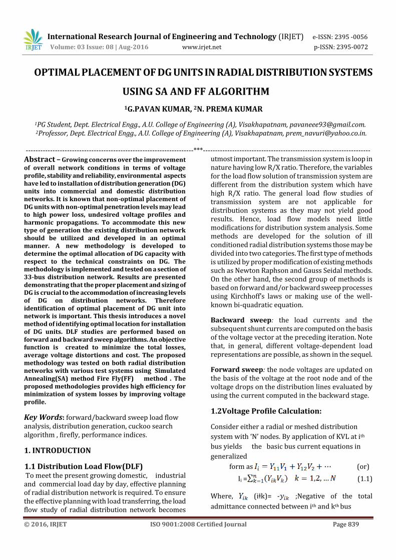
Below represents various waveforms with and without DG using Simulated Annealing with Loss sensitivity Factor(LSF). DG is placed at bus 7.

4.1 VOLTAGE MAGNITUDE

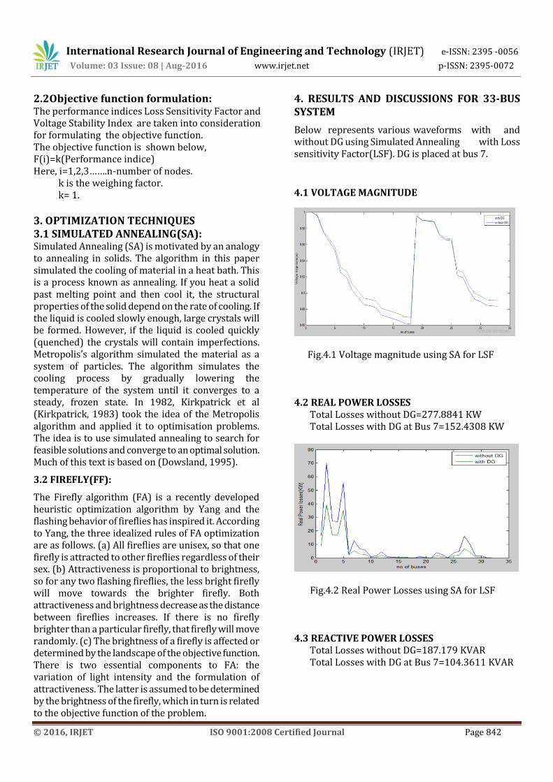
Fig.4.1 Voltage magnitude using SA for LSF 4.2 REAL POWER LOSSES Total Losses without DG=277.8841 KW Total Losses with DG at Bus 7=152.4308 KW

Fig.4.2 Real Power Losses using SA for LSF 4.3 REACTIVE POWER LOSSES Total Losses without DG=187.179 KVAR Total Losses with DG at Bus 7=104.3611 KVAR




Fig.4.3 Reactive Power Losses using SA for LSF Below represents various waveforms with and without DG using Simulated Annealing with Voltage Stability Index. DG is placed at bus 17.


Fig 4.4 Voltage magnitude using SA for VSI 4.5 REAL POWER LOSSES Total Losses without DG=277.8841 KW Total Losses with DG at Bus 17=156.5376 KW

Fig4.5 Real Power losses using SA for VSI 4.6 REACTIVE POWER LOSSES Total Losses without DG=187.179 KVAR Total Losses with DG at Bus 17=108.4409 KVAR

Fig 4.6 Reactive Power Losses using SA for VSI Below represents various waveforms with and without DG using Firefly Algorithm with Loss Sensitivity Factor. DG is placed at bus 12.


Fig 4.7 Voltage magnitude using Firefly for LSF

4.8 REAL POWER LOSSES

Total Losses without DG=277.8841 KW Total Losses with DG at Bus 12=152.5645 KW

Fig 4.8 Real Power Losses using FF for LSF

4.9 REACTIVE POWER LOSSES

Total Losses without DG=187.179 KVAR Total Losses with DG at Bus 12=104.4582 KVAR




Fig 4.9 Reactive Power Losses using FF for lsf

Below represents various waveforms with and without DG using Firefly Algorithm with Voltage Stability Index. DG is placed at bus 17.


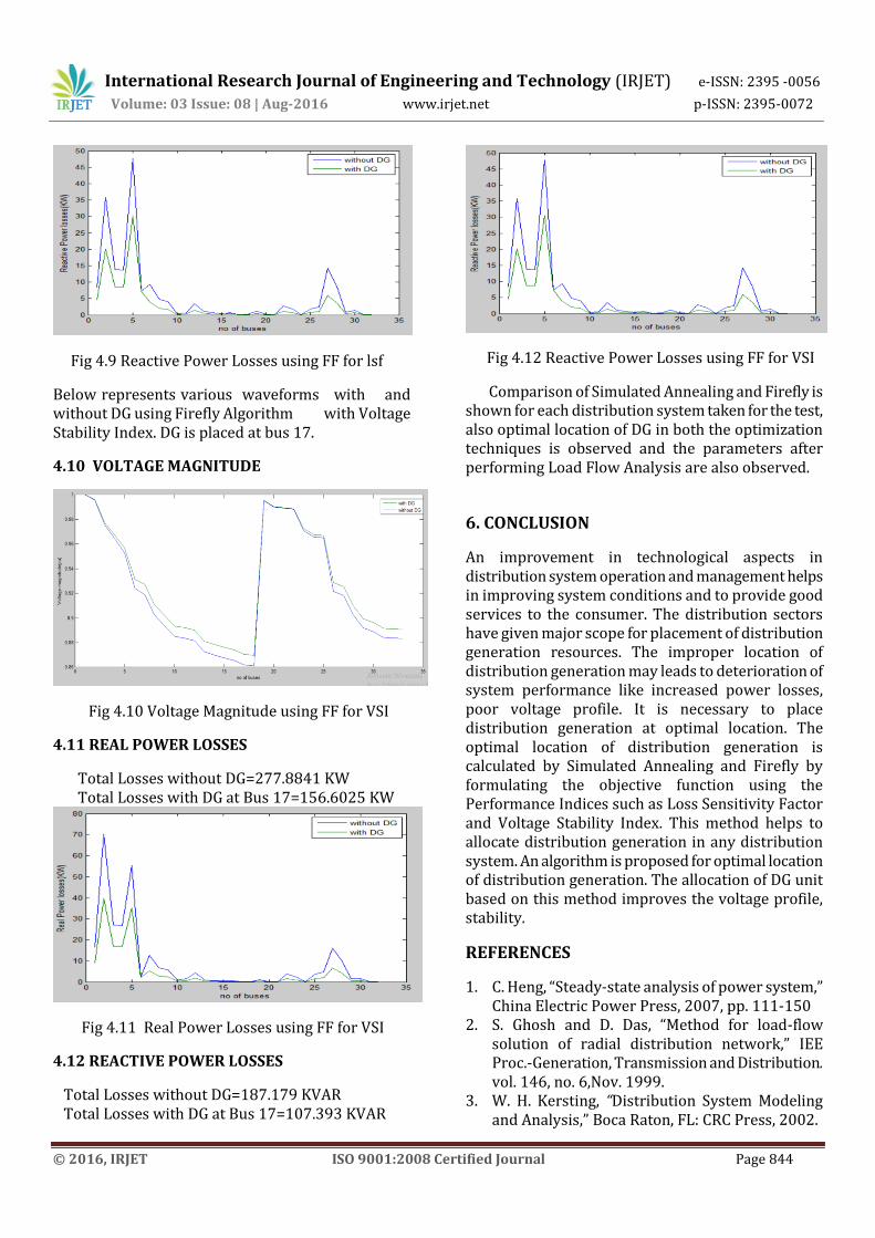
Fig 4.10 Voltage Magnitude using FF for VSI

4.11 REAL POWER LOSSES

Total Losses without DG=277.8841 KW Total Losses with DG at Bus 17=156.6025 KW

Fig 4.11 Real Power Losses using FF for VSI

4.12 REACTIVE POWER LOSSES

Total Losses without DG=187.179 KVAR Total Losses with DG at Bus 17=107.393 KVAR

Fig 4.12 Reactive Power Losses using FF for VSI

Comparison of Simulated Annealing and Firefly is shown for each distribution system taken for the test, also optimal location of DG in both the optimization techniques is observed and the parameters after performing Load Flow Analysis are also observed.

6. CONCLUSION

An improvement in technological aspects in distribution system operation and management helps in improving system conditions and to provide good services to the consumer. The distribution sectors have given major scope for placement of distribution generation resources. The improper location of distribution generation may leads to deterioration of system performance like increased power losses, poor voltage profile. It is necessary to place distribution generation at optimal location. The optimal location of distribution generation is calculated by Simulated Annealing and Firefly by formulating the objective function using the Performance Indices such as Loss Sensitivity Factor and Voltage Stability Index. This method helps to allocate distribution generation in any distribution system. An algorithm is proposed for optimal location of distribution generation. The allocation of DG unit based on this method improves the voltage profile, stability.

REFERENCES

1. C. Heng, “Steady-state analysis of power system,” China Electric Power Press, 2007, pp. 111-150

2. S. Ghosh and D. Das, “Method for load-flow solution of radial distribution network,” IEE Proc.-Generation, Transmission and Distribution. vol. 146, no. 6,Nov. 1999.

3. W. H. Kersting, “Distribution System Modeling and Analysis,” Boca Raton, FL: CRC Press, 2002.




4. D. Shirmohammadi, H. W. Hong, A. Semlyen, and G. X. Luo, “A compensation- based power flow method for weakly meshed distribution and transmission networks,” IEEE Trans. Power Syst., vol. 3, no. 2, pp. 753–762, May 1988.

5. A. Alsaadi, and B. Gholami,“An Effective Approach for Distribution System Power Flow Solution,” World Academy of Science, Engineering and Technology 28 2009, pp.732-736.

6. U. Eminoglu and M. H. Hocaoglu, “Distribution Systems Forward/Backward Sweep-based Power Flow Algorithms: A Review and Comparison Study,” Electric Power Components and Systems, 2009, pp.91-110.

7. Aarts, E.H.L., Korst, J.H.M. 1989. Simulated Annealing and Boltzmann Machines. Wiley, Chichester.

8. Connolly, D.T. 1990. An Improved Annealing Scheme for the QAP. EJOR, 46, 93-100

9. Dowsland, K.A. 1995. Simulated Annealing. In Modern Heuristic Techniques for Combinatorial Problems (ed. Reeves, C.R.), McGraw-Hill, 1995

10. Johnson, D.S., Aragon, C.R., McGeoch, L.A.M. and Schevon, C. 1991. Optimization by Simulated Annealing: An Experimental Evaluation; Part II, Graph Coloring and Number Partitioning. Operations Research, 39, 378-406

11. Kirkpatrick, S , Gelatt, C.D., Vecchi, M.P. 1983. Optimization by Simulated Annealing. Science, vol 220, No. 4598, pp671-680

12. Mitra, D., Romeo, F., Sangiovanni-Vincentelli, A. 1986. Convergence and Finite Time Behavior of Simulated Annealing. Advances in Applied Probability, vol 18, pp 747-771

13. A. Rana, A.E. Howe, L.D. Whitley and K. Mathias. 1996. Comparing Heuristic, Evolutionary and Local Search Approaches to Scheduling. Third Artificial Intelligence Plannings Systems Conference (AIPS-96)

14. Russell, S., Norvig, P. 1995. Artificial Intelligence A Modern Approach. Prentice-Hall

15. Rutenbar, R.A. 1989. Simulated Annealing Algorithms : An Overview. IEEE Circuits and Devices Magazine, Vol 5, No. 1, pp 19-26

16. Bonabeau E., Dorigo M., Theraulaz G., Swarm Intelligence: From Natural to Artificial Systems. Oxford University Press, (1999).

17. Chattopadhyay R., A study of test functions for optimization algorithms, J. Opt. Theory Appl., 8, 231-236 (1971).

18. Deb. K., Optimisation for Engineering Design, Prentice-Hall, New Delhi,(1995).

19. Goldberg D. E., Genetic Algorithms in Search, Optimisation and MachineLearning, Reading, Mass.: Addison Wesley (1989).

OPTIMAL PLACEMENT OF DG UNITS IN RADIAL ... PLACEMENT OF DG UNITS IN RADIAL DISTRIBUTION SYSTEMS...

Documents

Transcript of OPTIMAL PLACEMENT OF DG UNITS IN RADIAL ... PLACEMENT OF DG UNITS IN RADIAL DISTRIBUTION SYSTEMS...