Optimal Oil Production and the World Supply of Oil

Nikolay Aleksandrov, Raphael Espinoza, and Lajos Gyurkó

WP/12/294

© 2012 International Monetary Fund WP/12/294

IMF Working Paper

Research Department

Optimal Oil Production and the World Supply of Oil

Prepared by Nikolay Aleksandrov, Raphael Espinoza, and Lajos Gyurkó1

Authorized for distribution by Atish Rex Ghosh

December 2012

Abstract

We study the optimal oil extraction strategy and the value of an oil field using a multiple real option approach. The numerical method is flexible enough to solve a model with several state variables, to discuss the effect of risk aversion, and to take into account uncertainty in the size of reserves. Optimal extraction in the baseline model is found to be volatile. If the oil producer is risk averse, production is more stable, but spare capacity is much higher than what is typically observed. We show that decisions are very sensitive to expectations on the equilibrium oil price using a mean reverting model of the oil price where the equilibrium price is also a random variable. Oil production was cut during the 2008–2009 crisis, and we find that the cut in production was larger for OPEC, for countries facing a lower discount rate, as predicted by the model, and for countries whose governments’ finances are less dependent on oil revenues. However, the net present value of a country’s oil reserves would be increased significantly (by 100 percent, in the most extreme case) if production was cut completely when prices fall below the country's threshold price. If several producers were to adopt such strategies, world oil prices would be higher but more stable.

JEL Classification Numbers: C61 ; Q30 ; Q43 Keywords: Oil production ; Real Options ; Capacity Expansion ; Equilibrium Price of Oil; OPEC Author’s E-Mail Addresses: nikolay.aleksandrov@chch.oxon.org ; respinoza@imf.org ; gyurko@maths.ox.ac.uk

1 We are grateful for comments and suggestions from two anonymous referees, Christian Bender, Ben Hambly, Vicky Henderson, Sam Howison, Robert Kaufmann, Rick van der Ploeg, Oral Williams, and seminar and conference participants at Oxford, Princeton, the IMF, the EEA Annual Meeting and the ECB Workshop on Coping with Volatile Oil and Commodity Prices.

This Working Paper should not be reported as representing the views of the IMF. The views expressed in this Working Paper are those of the author(s) and do not necessarily represent those of the IMF or IMF policy. Working Papers describe research in progress by the author(s) and are published to elicit comments and to further debate.

2

Contents Page

I. Introduction ............................................................................................................................4 

II. Related Literature ..................................................................................................................5 A. Optimal Oil Production .............................................................................................5 B. Numerical Solutions for Real Options ......................................................................6 

III. Model Formulation and Numerical Solution .......................................................................7 A. Model Formulation ...................................................................................................7 B. Numerical Solution ...................................................................................................8 

IV. Oil Price and Extraction Costs Models ..............................................................................10 

V. Learning the Size of Reserves .............................................................................................12 

VI. Application ........................................................................................................................13 

VII. Results ..............................................................................................................................14 

VIII. Limitations of the Model .................................................................................................18 

IX. Determinants of Production Policies during the 2008–2009 Crisis...................................19 

X. Concluding Remarks and the World Supply of Oil ............................................................21  Tables 1. Parameters of the Oil Price Process (OLS on Yearly Data for the Period 1957–2008) ......10 2. Parameters of the Schwartz-Smith (2000) Price Process Estimated on Futures Data .........11 3. Annualized Parameters of the Extraction Cost Process (OLS on quarterly Data for the Period 1999–Q1 to 2009–Q1 ...............................................................................................11 4. Model for Proven Reserves (Standard Errors in Parentheses ..............................................14 5. Oil Production Capacity ................………...........................................................................15 6. Added Value by Expanded Capacity…….… ......................................................................16 7. Added Value by Expanded Capacity and Increased Access to Reserve ..............................17 8. Determinants of Cuts in Production During the Crisis of 2008–2009 .................................20 References ................................................................................................................................23

3

Figures 1. Standard Deviation of Change in Reserves .........................................................................27 2. Optimal Extration—Brazil and U.A.E .................................................................................27 3. Sensitivity to Key Parameters ..............................................................................................28 4. Sensitivity to Key Parameters ..............................................................................................29 5. Determinants of the Cut in Oil Production During the Crisis of 2008–2009 ......................29 6. World Oil Market ................................................................................................................30

I. INTRODUCTION

In this paper we investigate the optimal oil extraction strategy of a small oil producer facinguncertain oil prices. We use a multiple real option approach. Extracting a barrel of oil issimilar to exercising a call option, i.e. oil production can be modeled as the right to produce abarrel of oil with the payoff of the strategy depending on uncertain oil prices. Production isoptimal if the payoff of extracting oil exceeds the value of leaving oil under the ground forlater extraction (the continuation value). For an oil producer, the optimal extraction pathcorresponds to the optimal strategy of an investor holding a multiple real option with finitenumber of exercises (finite reserves of oil). At any single point in time, the oil producer isalso limited in the number of options he can exercise, because of capacity constraints.

Our first contribution is to present the solution to the stochastic optimization problem as anexercise rule for a multiple real option and to solve the problem numerically using the MonteCarlo methods developed by Longstaff and Schwartz (2001), Rogers (2002), and extended byAleksandrov and Hambly (2010), Bender (2011), and Gyurko, Hambly and Witte (2011).The Monte Carlo regression method is flexible and it remains accurate even forhigh-dimensionality problems, i.e. when there are several state variables, for instance whenthe oil price process is driven by two state variables, when extraction costs are stochastic, orwhen the size of reserves is a random variable.

We solve the real option problem for a small producer (with reserves of 12 billion barels) andfor a large producer (with reserves of 100 bilion barrels) and compute the threshold belowwhich it is optimal to defer production. In our baseline model, we find that the smallproducer should only produce when prices are high (higher than US$73 per barrel at 2000constant prices), whereas for the large producer, full production is optimal as soon as pricesexceed US$39. Optimal production is found to be volatile given the stochastic process of oilprices. As a result, we show that the net present value of oil reserves would be substantiallyhigher if countries were willing to vary production when oil prices change. This result hasimportant implications for oil production policy and for the design of macroeconomicpolicies that depend on inter-temporal and inter-generational equity considerations. It alsoimplies that the world supply curve would be very elastic to prices if all countries wereoptimizing production as in the baseline model — and as a result, prices would tend to behigher but much less volatile.

We investigate why observed production is not as volatile as what is predicted by the baselinecalibration of the model. One possible explanation is that producers are risk averse. Underthis assumption, production is accelerated and is more stable, but a risk averse producershould also maintain large spare capacity, a result at odds with the evidence that oil producersalmost always produce at full capacity. A second potential explanation is that producers areuncertain about the actual size of their oil reserves. Using panel data on recoverable reserves,we show however that, historically, this uncertainty has been diminishing with time andtherefore this explanation is incomplete, since even mature oil exporters maintain low sparecapacity. A third explanation may be that the oil price process, and in particular theequilibrium oil price, is unknown to the decision makers. Indeed, the optimal reaction to an

5

increase in oil prices depends on whether the price increase is perceived to be temporary or toreflect a permanent shift in prices. If shocks are known to be primarily temporary, productionshould increase in the face of oil price increases. But if shocks are thought to beaccompanied by movements in the equilibrium price, the continuation value jumps at thesame time as the immediate payoff from extracting oil. In that case an increase in price maynot result in an increase in production. Faced with uncertain views on the optimal strategy,the safe decision might well be to remain prudent with changes in production.

In practice, world oil production is partially cut in the face of negative demand shocks. Thelast section of the paper investigates whether the reduction in oil production during the2008–2009 crisis can be explained by the determinants predicted by the model. We find thatthe cut in production was larger for OPEC, for countries facing a lower discount rate, aspredicted by the model, and for countries with government finances less dependent on oilrevenues.

Section 2 provides a survey of the related literature on optimal production and real options,while Sections 3, 4 and 5 cover the model formulation and calibration. Section 6 describesbriefly the oil sector in the two countries used as applications. Sections 7 presents the basicset of results and Section 8 discusses some limitations of the model. Section 9 investigatesthe determinants of production strategies during the 2008–2009 crisis and Section 10concludes on the price-elasticity of the world supply of oil.

II. RELATED LITERATURE

A. Optimal Oil Production

The study of the economy of non-renewable resource extraction started with Hotelling(1931), who showed in a deterministic general equilibrium model that the price of theresource would grow at the rate of interest in competitive markets with constant extractioncosts. General equilibrium models later included the effect of uncertainty in technology, thesize of the resources, or the availability of substitutes. Partial equilibrium models in whichthe prices are given, but the decision to extract is a function of the stochastic price process,have a shorter history in the non-renewable resource literature, starting with Tourinho(1979a). Tourinho (1979a, 1979b) analyzed for the first time the valuation of resources in thecontext of a real ‘call’ option to exploit a field, using the Black and Scholes framework.

Paddock, Siegel and Smith (1988) later developed a model that became a popular approachfor decisions on upstream oil investments, in which a company has the option to explore anarea and in case oil is discovered, to commit to an immediate development investment beforea given date (the time to expiration). If the firm does not exercise the option to develop thefield until this date, the firm must return the concession rights back to a national authority.2

2Real option models are surveyed in Dixit and Pindyck (1994) and, for applications to oil investments, in Dias(2004).

6

The model took into consideration resource depletion when estimating the value of the oilfield. However, the issue of when to extract the resource after the field is developed iscompletely absent since the only decision to take is the optimal timing to develop the field.

Cherian et al. (1998) studied optimal production of a nonrenewable resource as a controlproblem in continuous time. The authors solved the Bellman nonlinear partial differentialequation (PDE) numerically using the Markov chain approximation technique of Kushner(1977) and Kushner and Dupuis (1992). The cost of extraction in Cherian et al. (1998) is afunction of time, the extraction rate and the total extracted amount, a model that fits wellextraction costs for ore mining. However, a drawback of these numerical solutions to theBellman PDEs is that they are feasible only for problems with low dimensionality, and it istherefore difficult to solve the problem with two-factor oil price processes, stochasticextraction costs, or stochastic reserves.

Work close to ours in terms of modeling assumptions is Caldentey et al. (2006), who studythe optimal operation of a copper mining project when the copper spot price follows a meanreverting stochastic process. The project is modeled as a collection of blocks (minimalextraction units) each with its own mineral composition and extraction costs. The authors areinterested in maximizing the economic value of the project by controlling the sequence andrate of extraction as well as investing on costly capacity expansions. Our model is moregeneral since we allow for multiple exercise (i.e. the company can choose to extract differentvolumes every period) and because in our model the firm is able to scale down production.

We provide a multiple real option solution to the stochastic optimization problem. Productioncapacity is exogenous but it is a function of time. We also assume there is a minimumextraction capacity that is non-zero. This assumption captures the fact that some minimalextraction is often needed to finance the functioning of the firm, the transfers to thegovernment, or even the spending of the government in countries where oil proceeds are themajor source of government revenues.

B. Numerical Solutions for Real Options

The optimal extraction problem faced by an oil producer is similar to many other stochasticoptimization problems described in macroeconomics (e.g. investment under uncertainty, seefor instance Sakar, 2000), in finance (e.g. the choice of bank capital given uncertain cashflows, see Milne and Whalley, 2001, and Peura and Keppo, 2006) and in the natural resourcesliterature (e.g. the optimal exploitation of forest, see Alvarez and Koskela, 2006). Closedformulae for the price of early exercise options have not been derived yet, even for thesimplest cases. In particular, there is no analytical method for solving multiple real optionproblems. The difficulty in any option model is to compute the continuation value (theexpected value of delaying the extraction of a barrel). Following the analysis of Arrow,Blackwell and Girshick (1949), the problem was recognized and discussed as an abstractoptimal stopping problem by Snell (1952), and the first application of the optimal stoppingproblem to finance appeared in Bensoussan (1984).

7

The literature has however suggested various analytical approximations and numericalmethods. For most option pricing problems, three numerical methods are available: lattices,finite difference, and Monte Carlo methods.3 The first two approaches work best for simpleoptions on a single underlying (a single state variable). When there are more state variablesand the dimension of the problem increases, however, the Monte Carlo approach is preferredas the performance of the lattice and finite difference schemes is poor (the computationaleffort with these two methods grows exponentially with the number of state variables).

The first attempt to apply Monte Carlo techniques to American option pricing is due to Tilley(1993), while Broadie and Glasserman (1997) developed the first algorithm in which thesuggested lower and upper bound estimates are proved to converge to the true value. Theirapproach can also deal with high-dimensional American options, but the computational effortstill grows exponentially with the number of possible exercise dates. There has been arenewal of interest in the recent years for these methods (Jaillet, Ronn and Tompaidis, 2004;Meinshausen and Hambly, 2004; Carmona and Touzi, 2008). The solution we use wasdeveloped in Aleksandrov and Hambly (2010), Bender (2011) and Gyurko, Hambly andWitte (2011) as an extension to the Monte Carlo method proposed by Longstaff and Schwartz(2002) and Tsitsiklis and van Roy (2001).

The method relies on approximating the value function by linear regression on a suitablespace of basis functions (see section 3 for more details). The fitted value from the regressiongives an estimate for the continuation value. By construction this optimal stopping policygives a lower bound for the option price — only the exact decision rule would give themaximum value and an approximation can only give a lower estimate. The method iscomparatively easy to implement and for properly chosen regression functions gives a goodestimate of the value function, even with models with several states variables (seeGlasserman, 2003).

III. MODEL FORMULATION AND NUMERICAL SOLUTION

A. Model Formulation

We present here the stochastic optimization problem. We consider an economy in discretetime defined up to a finite time horizon of T years at which we assume reserves will bedepleted.4 The maximum yearly capacity for extraction (the production capacity) is assumedto be exogenous, although in practice it would be a function of past investments. Productioncapacity is noted kt (in billion barrels per year), t = 1, 2, ..., T .5 The optimal extraction

3A new method based on generalized linear complementarity problems (GLCPs) has recently been proposed byNagae and Akamatsu (2008).

4In several of our applications, we assume that countries extract every year a minimum amount of barrels, inwhich case extraction occurs indeed over a finite horizon.

5kt must be a multiple of the discretization unit that we use and that represents one real option to extract oil.

8

strategy maximizes the discounted utility of the cash flow from oil sales V ∗,m,kt at time t,subject to the capacity constraints k = {k0, k1, k2, ..., kT} and to the total oil reservesconstraint m. If the oil producer decides to extract one barrel of oil at time t, the profit is St,where St is the price of oil (net of the extraction cost ct). Profits are always positive when theproducer decides to extract oil since she is not forced to produce making losses. We abstractfrom the costs of shutting down an oil production unit.

We assume that oil prices follow a discrete Markov chain process (St)t=0,1,...,T ∈ Rd (wecome back to the discussion on oil prices in section IV). We define an extraction policy πk tobe a set of ‘stopping’ times (i.e. times at which the real options are exercised) {τi}mi=1,τ1 ≤ τ2 ≤ · · · ≤ τm, such that the number of exercises (i.e. annual production) is lower thanproduction capacity each year: #{j : τj = s} ≤ ks.

The instantaneous utility of extracting ht units of oil on top of the minimum level l of annualextraction at time t is denoted by u((ht + l)St) where u(x) = x1−γ−1

1−γ is the Constant RelativeRisk Aversion utility function defined over R+, and γ ≥ 0, γ 6= 1 is the coefficient of riskaversion.6 1/Bt is the discount factor, i.e. if the rate of impatience is equal to a constantrisk-free rate r, Bt = ert. Then, the optimal consumption problem can be formulated asfollows.

Definition 1.

V ∗,m,kt = supπk

V πk,mt = sup

πk

Et

[m∑i=1

u((hτi + l)Sτi)

B(t, τi)

].

The corresponding optimal policy is π∗ = {τ ∗1 , τ ∗2 , ..., τ ∗m}.

B. Numerical Solution

We estimate the optimal extraction strategy using Monte-Carlo techniques. In particular, ournumerical approach is based on the dynamic programming formulation:

V ∗,n,kt (s) = sup0≤h≤min{kt,n}

{u((h+ l)s) + 1

Bt,t+1E[V ∗,n−h,kt+1 (St+1)

∣∣∣St = s]}

(1)

for t = 0, . . . , T − 1 and V ∗,n,kT (s) = u(min{kT , n}s).The conditional expectation in (1), is approximated using least squares regression techniques.In the case where the level of reserves is assumed to change due to extraction only, we usethe approximation:

∀n, E[V ∗,n,kt+1 (St+1)

∣∣∣St = s]≈

k∑i=1

βnt,iψi(s) (2)

where the ψi are the basis functions that we use to approximate the value function. In all thespecifications, we use local functions (i.e. functions defined over intervals or boxes, in the

6When γ = 1, the utility function is defined as u(x) = log(x).

9

higher dimensional cases). In the baseline model, the basis functions are polynomials of theoil price and its logarithm, and when risk aversion is positive, different powers of the utilityfunction were included as well.

The least squares regression approach implies that the vector of regression coefficientsβnt = (βnt,1, . . . , β

nt,k)

T satisfies the linear equation

E[(φ1(St), . . . , φk(St))

T (φ1(St), . . . , φk(St))]βnt

= E[(φ1(St), . . . , φk(St))

T V ∗,n,kt+1 (St+1)]. (3)

In the case where the level of reserves follows a stochastic process, the dynamicprogramming formulation has to be refined for two reasons. First, the level of reserves mightdrop below the minimum extraction level l before the end of the time horizon. Second, wehave to take into account the autoregressive nature of the reserves process (see equation (9) inSection 5). These considerations lead to the following formulation:

V ∗kt (st, rt, rt−1) = supmin{rt,l}≤h≤min{l+kt,rt}

{u((h+ l)s)

+ 1Bt,t+1

E[V ∗,kt+1(St+1, Rt+1, Rt)

∣∣∣St = st, Rt = rt − h,Rt−1 = rt−1

]}.

(4)

In this case, we approximate the continuation value by the following multivariate regression:

E[V ∗,kt+1(St+1, Rt+1, Rt)

∣∣∣St = s, Rt = r, Rt−1 = r]≈

k∑i=1

βnt,iψi(s, r, r). (5)

The set of basis functions included polynomials of the oil price, the log oil price and thereserve level and its lag. The vector of regression coefficients βnt = (βnt,1, . . . , β

nt,k)

T satisfiesthe linear equation

E[(φ1(St, Rt, Rt−1), . . . , φk(St, Rt, Rt−1))

T (φ1(St, Rt, Rt−1), . . . , φk(St, Rt, Rt−1))]βnt

= E[(φ1(St, Rt, Rt−1), . . . , φk(St, Rt, Rt−1))

T V ∗,n,kt+1 (St+1, Rt+1, Rt)]. (6)

The regression coefficients in (2) (respectively in (5)) are estimated by replacing theexpectations in (3) (and in (6)) by their Monte-Carlo estimates based on random grids andbackward recursion. This method is referred to as a priori and described in detail in Gyurko,Hambly and Witte (2011).

The numerical solution can be affected by three types of errors: (i) discretization errors thatcome from the transformation of a continuous time process into a discrete one (this can bereduced simply by reducing the length of the period); (ii) the projection error due to the fact

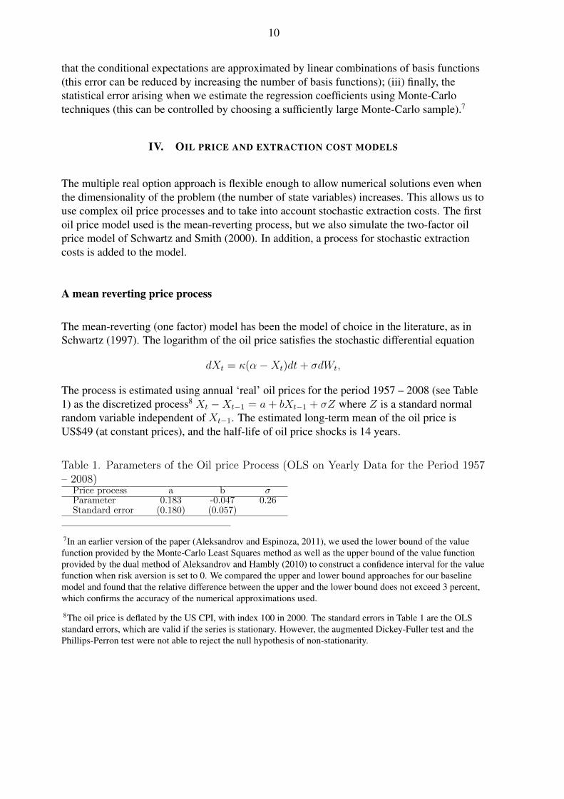
10

that the conditional expectations are approximated by linear combinations of basis functions(this error can be reduced by increasing the number of basis functions); (iii) finally, thestatistical error arising when we estimate the regression coefficients using Monte-Carlotechniques (this can be controlled by choosing a sufficiently large Monte-Carlo sample).7

IV. OIL PRICE AND EXTRACTION COST MODELS

The multiple real option approach is flexible enough to allow numerical solutions even whenthe dimensionality of the problem (the number of state variables) increases. This allows us touse complex oil price processes and to take into account stochastic extraction costs. The firstoil price model used is the mean-reverting process, but we also simulate the two-factor oilprice model of Schwartz and Smith (2000). In addition, a process for stochastic extractioncosts is added to the model.

A mean reverting price process

The mean-reverting (one factor) model has been the model of choice in the literature, as inSchwartz (1997). The logarithm of the oil price satisfies the stochastic differential equation

dXt = κ(α−Xt)dt+ σdWt,

The process is estimated using annual ‘real’ oil prices for the period 1957 – 2008 (see Table1) as the discretized process8 Xt −Xt−1 = a+ bXt−1 + σZ where Z is a standard normalrandom variable independent of Xt−1. The estimated long-term mean of the oil price isUS$49 (at constant prices), and the half-life of oil price shocks is 14 years.

Table 1. Parameters of the Oil price Process (OLS on Yearly Data for the Period 1957– 2008)

Price process a b σParameter 0.183 -0.047 0.26Standard error (0.180) (0.057)

7In an earlier version of the paper (Aleksandrov and Espinoza, 2011), we used the lower bound of the valuefunction provided by the Monte-Carlo Least Squares method as well as the upper bound of the value functionprovided by the dual method of Aleksandrov and Hambly (2010) to construct a confidence interval for the valuefunction when risk aversion is set to 0. We compared the upper and lower bound approaches for our baselinemodel and found that the relative difference between the upper and the lower bound does not exceed 3 percent,which confirms the accuracy of the numerical approximations used.

8The oil price is deflated by the US CPI, with index 100 in 2000. The standard errors in Table 1 are the OLSstandard errors, which are valid if the series is stationary. However, the augmented Dickey-Fuller test and thePhillips-Perron test were not able to reject the null hypothesis of non-stationarity.

11

Table 2. Parameters of the Schwartz-Smith (2000) Price Process Estimated on FuturesData

Parameters κ σχ µξ∗ σξ ρξχEstimate 1.49 0.286 0.0115 0.145 0.3Standard error (0.03) (0.01) (0.0013) (0.05) (0.044)

Table 3. Annualized Parameters of the Extraction Cost Process (OLS on QuarterlyData for the Period 1999–Q1 to 2009–Q1)

Cost process c σcParameter 0.08 0.39Standard error (0.06)

A model with stochastic equilibrium price

The mean reversion model assumes that the long-term mean (or the equilibrium level) of theoil price is known. Schwartz and Smith (2000) proposed a two-factor model for the oil pricethat captures uncertainty in the equilibrium oil price. More precisely, the logarithm of theprice Xt has two components: short-term deviations Yt, which follow a mean-revertingprocess (with mean 0), and the equilibrium level Mt, which is assumed to follow a Brownianmotion.

Xt = Yt +Mt

dYt = −κYtdt+ σχdWt

dMt = µξ∗dt+ σξdWt

(7)

In addition, the shocks in the short term are correlated with the shocks to the equilibriumprice, i.e. corr(Wt, Wt) = ρξχ. The model is implemented using the followingdiscretization.9

{Yt = Yt−1(1− κ∆t) + σχ

√∆tZ

Mt = Mt−1 + µξ∗∆t+ σξ√

∆t(ρξχZ +√

1− ρ2ξχZ)(8)

where Z and Z are independent and normally distributed, and ∆t is set to 1. The parameterswe use are those estimated by Schwartz and Smith (2000) and presented in Table 2. Thehalf-life of short-term shocks is less than a year but the equilibrium price is also variable, witha volatility of 14.5 percent. In order to account for the two factor model in the Least SquaresMonte-Carlo algorithm, the two state variables are added to the set of basis functions ψ.

9The two factors are not observable, but Schwartz and Smith (2000) estimate them using spot and future pricesover the period 1990-1996.

12

Oil prices correlated with extraction costs

Extraction costs can reach high levels. For instance, the cost of extraction for PetroleoBrasileiro S.A. (Petrobras) exceeded US$30 per barrel in 2008. These costs can be added tothe model assuming they follow a geometric Brownian motion:

logCt = logCt−1 + c+ σc(ρZ +√

1− ρ2Z),

where Z is a standard normal random variable independent of Z, and ρ is the correlationbetween oil prices and extraction costs. The correlation between oil prices and the extractioncosts faced by Petrobras has been low because the government contributed to the cost, butwhen taking into account this cost to the government, the correlation between quarterlypercentage changes is high; it exceeded 70 percent over the period 1999–2009. We firstestimate a discretized model log(Ct)− log(Ct−1) = c+ σcZ, with parameter estimatesshown in Table 3 and then investigate how positive correlations affect the optimal strategy.Again, the new state variable is added to the set of basis functions in the Least SquareMonte-Carlo algorithm.

V. LEARNING THE SIZE OF OIL RESERVES

Farzin (2001) argued that proven oil reserves are the output of a production process anddepend on the payoff (the oil price), past extraction (to capture depletion) and a level oftechnology. In particular, he estimated on U.S. data that a 10 percent increase in oil pricestriggers discoveries of 1 percent of additional reserves. Lund (2000) modeled a Bayesianlearning process in the amount of oil reserves. The prior distribution on oil reserves isupdated by information on the amount of oil extracted and the pressure of the well. In Lund(2000), when pressure declines, it indicates that the remaining volume of oil is neardepletion. If the pressure is constant, it indicates that the reserves are at least higher thanproduction and therefore the range of uncertainty in reserves declines with extraction.

We model reserves taking into account these findings. We estimate a model where increasesin reserves depend on the oil price, past extraction, time (which captures technologicalinnovations), and where the conditional variance of reserves is also a function of time. Thislater component proxies for learning in the size of reserves in the spirit of Lund (2000). Lund(2000)’s formulation for reserves is appropriate to model reserves of a specific field, but notfor a country as the model would not be able to capture potential discoveries in reserves dueto higher oil prices or better technology. A cursory look at the EIA data however confirmsthat uncertainty in reserves has been declining with time. Figure 1 shows that for the medianoil producer, the standard deviation of annual changes in proven reserves has decreased byabout 50 percent in 19 years. This discussion suggests the following model for reserves:

∆ log(Rt) = a0 + a1time+ a2 log(Pt−1) + a3∆ log(Rt−1) + a4CUMt−1 + εt (9)

13

where the conditional variance of the normally-distributed εt (given available information) isa function of time:10

εt ∼ N(0, σ2t ) (10)

σ2t = exp(b0 + b1 time) (11)

The model is estimated on the proven reserves of crude oil from the EIA, for the panel of 98countries for which reserves data was available, over the period 1980–2009. After removingextreme changes in reserves that would not be realistic for relatively mature oil producers(higher than 50 percent and lower than 50 percent), the data still shows excess kurtosis of 6.5.This suggests that the model described by equation 9, with normally distributed errors, maybe improved by choosing a different specification for εt. We therefore estimated the model 9by quasi-maximum likelihood (Bollerslev and Wooldridge, 1992) assuming that εt isdistributed as a Student’s t distribution, with degrees of freedom v =3, v = 5 (our preferredspecification as it implies an excess kurtosis of 6 for εt), and v = 10 (closer to normaldistribution).

The results are shown in Table 4. Columns 1 to 3 show the most general model for differentdegrees of freedom of the Student’s t distribution. The coefficients for the variables thatsignificant are robust, and we decide to stick to a model with v = 5. We use aGeneral-To-Specific approach and drop the least significant variables (columns 4 to 6).Reserves depletion (CUM )11 and oil prices were not found to be significant. However, thepast change in oil reserves was significant and the time trend in the variance equation washighly significant, for all our specifications. Column 7 shows that there are large differencesin the variance equation for countries with reserves larger than 5 billion barrels. We thereforeestimate a separate model for these countries, shown in column 8, and use these estimates tocalibrate our model of reserves. The coefficient of the time trend in the variance equationimplies that every year the conditional variance in the volume of proven reserves is reducedby around 4.5 percent. This corresponds to a 50 percent decline of the standard deviation in15 years - in line with what can be deduced by a reading of Figure 1.

VI. APPLICATION

We apply the model to two countries, one with small reserves and one with large reserves.We assume in all calculations that the extraction decisions are made on a yearly basis. Thesmallest unit that is used to change production is 0.2 billion barrels per year, equivalent to0.55 million barrels per day. We also make the assumption that each country extracts at least0.5 billion barrels per year to finance operations and ensure a minimum of revenues. For thecountry with small reserves, the time horizon chosen is 16 years in the model with known

10time is a linear trend that takes the value 0 in 1980 and 32 in 2012, which is the first year of the simulationspresented in section VI.

11Farzin (2001) uses both CUMt−1 and CUMt−2 but the two variables are almost identical in our sample so wedropped CUMt−2.

14

Table 4. Model for Proven Reserves (Standard errors in parentheses, *** p < 0.01, **p < 0.05, * p < 0.1)

(1) (2) (3) (4)Level Eq. v= 3 v= 5 v= 10 v= 5

∆ logRt−1 0.0142** 0.0239** 0.0226 0.0239**(0.00622) (0.0118) (0.0192) (0.0118)

CUMt−1 -1.65e-05 -2.07e-05 -4.99e-05(1.50e-05) (3.25e-05) (9.48e-05)

logPt−1 -0.000578 0.00262 0.00889 0.00265(0.00177) (0.00371) (0.00622) (0.00371)

logPt−2 -1.03e-05 -0.00402 -0.0134** -0.00402(0.00160) (0.00361) (0.00634) (0.00361)

time 0.000154 0.000100 -7.18e-05 9.65e-05(0.000120) (0.000171) (0.000235) (0.000170)

Constant -0.00100 0.00272 0.0159 0.00263(0.00246) (0.00598) (0.0110) (0.00597)

Variance Eq.

time -0.162*** -0.109*** -0.0745*** -0.109***(0.0210) (0.0156) (0.0134) (0.0155)

Const. -3.494*** -4.000*** -4.128*** -4.000***(0.256) (0.218) (0.197) (0.218)

time I[res>5]

Const. I[res>5]

Obs. 1,611 1,611 1,611 1,611

(5) (6) (7) (8)Level Eq. v= 5 v= 5 v= 5 v= 5

(res> 5 bn b)

∆ logRt−1 0.0197* 0.0195* 0.0144 0.0473*(0.0112) (0.0110) (0.0101) (0.0248)

CUMt−1

logPt−1 0.000356(0.00186)

logPt−2

time 0.000121 0.000158(0.000155) (0.000125)

Constant -0.00376 -0.00342(0.00522) (0.00287)

Variance Eq.

time -0.113*** -0.114*** -0.147*** -0.0453**(0.0143) (0.0142) (0.0207) (0.0204)

Const. -3.944*** -3.950*** -3.321*** -5.427***(0.192) (0.190) (0.239) (0.351)

time I[res>5] -2.120***(0.423)

Const. I[res>5] 0.103***(0.0292)

Obs. 1,777 1,802 1,802 565

reserves, which leaves us with 25 units of 0.2 billion barrels per year (after the minimalextraction rate of 0.5 billion barrels per year are subtracted). In the model with unknownreserves, the horizon is extended to 25 years. For the country with large reserves, we considera time horizon of 100 years and 240 extractable units. We assume production capacityincreases for the next twenty years (see Table 5), and we assume capacity is constant after2030. The calibration used for the numerical results is reported in the same table.

VII. RESULTS

The model parameters used to determine the optimal policy are assumptions of the model.We discuss the changes in optimal policy when these parameters change. The baseline model

15

Table 5. Oil production capacityExtraction capacity 2010 2015 2020 2025 2030In billion barrels per year 1.0 1.3 1.4 1.6 1.7Calibration, in units (1 unit = 0.2 billion barrels) 5 6 7 8 8

is a model with risk aversion set to 0, mean reverting oil prices, no extraction costs, andknown reserves. We investigate the dependence of optimal policy on: (i) the expectedvolatility of oil prices ; (ii) interest rates; (iii) the size of reserves; (iv) production capacity;(v) risk aversion; (vi) extraction costs and (vii) uncertainty in the size of reserves.

Baseline. We show in the left hand side chart of Figure 2 the optimal extraction path for thesmall producer for a hypothetical oil price simulated using the mean-reverting oil pricemodel described earlier. Extraction at the minimum level remains optimal for three years,until the oil price exceeds US $70 in the fourth year of the simulation. A striking feature ofthe optimal extraction strategy for both small and large producers, and that was found withmost simulations of the oil price under the baseline model, is that production is quite volatile(although we did not impose a so-called ’bang-bang’ solution, as will be clearer whenlooking at the impact of risk aversion). This result is at odds with the actual behavior of oilproducers, who most often extract at full capacity until oil fields are exhausted. We discuss inthe remainder of the paper whether different specifications of the model yield more realisticresults.

Sensitivity to the volatility of oil prices. We show in the top left chart of Figure 3 thesensitivity of the solution to different assumptions on expected oil price volatility, for a givenrealization of the oil price path. As was emphasized by the ‘waiting to invest’ literature, highvolatility makes it optimal to defer the exercise of options. During the first four years of thesimulation, as oil prices are low, it is only optimal to extract oil for a producer that wouldbelieve that oil price volatility is low (σ = 0.13). A producer who thinks prices are stablewould always find it optimal to extract at full capacity and would quickly exhaust its oil field,missing the opportunity to extract when prices are higher. On the other hand, a producer whothinks volatility is 0.52 would delay extraction until it is forced to extract (when the contractto exploit the field expires).

Sensitivity to the real interest rate. Dependence on the real interest rate is shown in the topright chart of Figure 3. In these simulations, exercise occurs earlier at higher interest rates, aresult that differs from the one found for simple European call options. In the Black-Scholesformula, using the risk neutral form of the stock price, the drift for the oil price is higher thehigher the interest rate, which implies that the underlying price goes above the strike withlarger (risk-neutral) probability when the interest rate is higher. As a result, the continuationvalue is higher when the interest rate is higher. In our model, the interest rate only appears inthe discount factor and has no impact on the drift of the oil price, which is why thecontinuation value can be lower with higher interest rates.

Sensitivity to the size of reserves. The threshold price at which production at full capacity isoptimal is of course a function of reserves. The right hand side chart of Figure 2 show that

16

the country with large resources (‘large producer’) should extract at full capacity for fairlylow oil prices. The threshold price for the country with smaller reserves (‘small producer’)was found to be US $73 (in 2000 terms, i.e. around US $95 of 2011).12 For the largeproducer, the threshold would be US $39 (around US $50 of 2011). However, we found thatsmaller differences in the amount of reserves (one to two billion barrels) do not changesignificantly the shape of the optimal production strategy (see third chart in Figure 3).

Impact of increasing capacity. We compute the increase in net present value of the oil fields(the value function when risk aversion is set to 0) that is obtained when increasing capacity,for a given amount of total reserves. The increase in NPV is our estimate of the shadow priceof the yearly production capacity constraint. This number can be used to assess theprofitability of a project for which investment costs are known. We consider two countrieswith oil reserves estimated at 5 and 10 billion barrels (25 and 50 units respectively).13 Theresults are presented in Table 6. A capacity expansion of 200 million barrels per year in 2025(1 additional unit in Year 15) improves the value of the oil reserves by US$ 2.1 billion, for acountry whose reserves are 5 billion barrels.14 The increase would reach US$ 6.27 billion fora country that holds 10 billion barrels. Additional capacity has more value for countries withlarger reserves, a result that, if it already existed, was not echoed in the oil productionliterature. The intuition is that the additional option provided by higher capacity has morevalue if it is available for many years and if production capacity was a tighter constraint attimes of high prices. Our results therefore suggest that project evaluation needs to beperformed in the context of the overall oil strategy of the country, since the viability andprofitability (i.e. net present value) of projects cannot be assessed project-by-project.However, the value of ‘optionality’ created by higher capacity is small compared with thevalue of reserves that are normally made available when new wells or platforms are open. Weshow in Table 7 the value of such a project if the additional reserves are worth 1 billionbarrels (5 units of 200 million barrels). The value of the project is now higher for the countrywith lower reserves because the value of optionality is dwarfed by the value of additional oilreserves, and an additional one billion barrels of oil reserves is worth more for a country thathas low reserves than for a country that has high reserves. Indeed, for a given finite horizonand a given production capacity, a country with low reserves can ‘distribute’ the extraction ofnewly-found reserves more optimally than a country that has high reserves.

Table 6. Added Value by Expanded Capacity.Year (unit = 0.2 bn bbl/year) 1-5 5 -10 10-15 15- 25 units 50 unitsCurrent capacity 3 4 5 5 US$ 325.9bn US$ 622.5bnIncreased capacity 3 4 5 6 US$ 328bn US$ 628.8bnAdded value US$ 2.1bn US$ 6.27bn

Risk Aversion. The fourth chart in Figure 3 shows how increasing risk aversion makesearlier production optimal. In the first periods of the simulation, production at full capacity

12US CPI inflation between 2000 and 2011 was 30 percent.

13The oil price process parameters are as before. We start with oil price S = 54.6. The time horizon in 100years.

14We assume that production capacity is maintained at the highest level after expansion, although productioncapacity is usually declining with time because of depletion.

17

Table 7. Added Value by Expanded Capacity and Increased Access to Reserves.Year (unit = 0.2 bn bbl/year) 1-5 5 -10 10-15 15- 25/30 50/55Current capacity 3 4 5 5 US$ 325.9bn US$ 622.5bnIncreased capacity 3 4 5 6 US$ 391.4bn US$ 685.2bnAdded value US$ 65.6bn US$ 62.7bn

becomes optimal with a small level of risk aversion because the utility costs of loweringproduction when income is low are high. Production is accelerated when risk aversion isincreased, a result similar to that of Alvarez and Koskela (2006). However, as prices increasein period 3, production is maintained at a lower but stable level, above minimum extraction,when risk aversion is higher. This allows the country to preserve its reserves and thereby to‘insure’ itself against future drops in the oil price. Although risk aversion might explain whyproduction is less volatile, risk-averse producers should maintain large spare capacity, aresult at odds with the evidence that only Saudi Arabia, of all producers, maintains sizablespare capacity.

Extraction Costs. Extraction costs, even when highly correlated with oil prices, do not affectsignificantly the optimal strategy because the net payoff of extracting a barrel of oil remainsvolatile.

Uncertainty in the size of oil reserves. We compute the optimal extraction strategy fordifferent calibrations of the reserves process. As is done with the oil price, the path ofdiscovery of reserves is kept identical across simulations, but the decision rules have beenestimated assuming different processes for reserves. The differences across simulations cantherefore be interpreted as due to the formation of expectations by the oil producer. First, wecompare a simulation where reserves are known (but moving with time) with a simulationwhere reserves are thought to follow the stochastic process described in equation 9, withshocks to reserves parameterized with a constant variance of 5 percent. The bottom rightchart in Figure 3 shows that additional uncertainty in the size of reserves triggers earlierextraction. The intuition behind this result is that since the life of the contract is finite, thereis an opportunity cost of delaying extraction if additional oil resources are found later.

Learning the size of oil reserves. Second, we show the optimal extraction policy fordifferent learning speeds (of the size of reserves). The first simulation assumes that thevariance of shocks to reserves is 5 percent in the first year and declines to reach 3.2 percent inyear 10 (‘slow learning’: the model for reserves was calibrated assuming b0 = −1.5 andb1 = −0.046 in equation 11). The second simulation assumes that the variance of shocks toreserves is also 5 percent in the first year but declines to 1.9 percent in year 10 (fast learning:the model for reserves was calibrating assuming b0 = 0.23; b1 = −0.1). We show two sets ofsimulations: one in which reserves are discovered (example (a); top left chart in Figure 4)and one in which reserves are depleted faster than in the simulation with known reserves(example (b); top right chart of Figure 4). The charts show that in the first period of themodel, fast learning tends to defer extraction, for the same reason that uncertainty tended toaccelerate extraction: the opportunity cost of delaying extraction if reserves are found later islower since the producer will learn quickly about the size of reserves. Production is also morestable after some years because reserves uncertainty is reduced considerably in 10 years.

18

VIII. LIMITATIONS OF THE MODEL

The previous section showed that the supply elasticity of the model is often much higher thanwhat can be inferred from the observed supply response to prices. Krichene (2005) indeedargued that short-term supply is insensitive to price. There are several potential explanationsto this finding, and we discuss below the three that we think are most relevant beforeinvestigating the determinants of oil production volatility empirically.

• There are technical limitations and fixed costs that reduce the benefits of varyingproduction. For instance, there is a minimum turn-down that is necessary to have theplant on, to avoid rusting, losing staff, etc. Similarly, if extraction costs are a functionof oil production, the solution of the model will differ somewhat and optimal oilproduction will be less volatile. However, these costs do not seem to have preventedseveral oil producers (with varied types of plants) to cut dramatically production duringthe recent crisis. According to the Joint-Oil Data Initiative (JODI) monthly database,the peak-to-through cut in oil production during the last crisis reached or exceeded 30percent in Azerbaijan, Brunei, Denmark, Malaysia, Norway and the UK.

• We have abstracted from re-investment costs to re-start production and from fixedoperational costs. Fixed operational costs do not affect the optimal strategy when thehorizon of exploitation is known, but they would matter if extending the life of a fieldwas possible, but costly for a variety of reasons. For instance, in countries such asBrazil or Norway, contracts on the exploitation of a field expire after 25-30 years, butcontracts might be extended (at some economically significant cost) after negotiatingwith the government.15

• The optimization model is not appropriate if a country’s discount rate is contingent onoil production. This will be the case for oil producers whose budget and externalaccounts are highly dependent on oil revenues. For such countries, cutting productionat the time prices are low will push those accounts in deficit and trigger borrowing atincreased rates, which governments and oil companies will be unwilling to do.However, given the significant losses in NPV (130 percent in the extreme case, seesection X), strategies that lead to more volatile production should be considered,especially for producers with larger reserves and for those who already accumulatedlarge financial reserves.

• Decisions are very sensitive to expectations of the equilibrium oil price, as can be seenfrom the bottom left chart in Figure 4. When the decision rule is computed based on anequilibrium oil price of US$30, production at full capacity is optimal for 8 years in arow (given the realized price shown in the figure), even though the half-life is 14 years(and therefore even though temporary shocks have a large effect of the continuationvalue). Decision making becomes even more complex when oil prices follow amean-reverting model with stochastic equilibrium price (the Schwartz and Smith

15We are grateful to an anonymous referee for pointing this to us.

19

(2000) model). The bottom right chart of Figure 4 shows a simulated path of anobserved oil price together with the underlying unobserved equilibrium price, wherethe simulation parameters are those shown in Table 2. The series labeled ρξχ = 0.3shows optimal extraction when the decision rules have been calculated using the MonteCarlo simulations based on these same parameters. In that sense, this series shows theoptimal extraction when expectations are based on the ‘correct’ model of oil prices.Roughly speaking, extraction is optimal when spot prices exceed equilibrium prices.The series labeled ρξχ = 0.8 shows optimal extraction when the decision rules havebeen calculated using the Schwartz-Smith model, but with the correlation betweenshort-term shock and equilibrium shocks set to 0.8. The series therefore shows theoptimal extraction when the decision maker expects observed short-term shocks to beaccompanied by shocks to the equilibrium price of oil. As a result, in the first 10 yearsof the production horizon, production is increased slowly even as prices go up becausethe continuation value increases when shocks are thought to be permanent (since thereis a value to wait). Faced with uncertainty on the right model of oil prices, the prudentdecision may be to maintain a relatively stable level of production.

IX. DETERMINANTS OF PRODUCTION POLICIES DURING 2008–2009 CRISIS

We finally investigate statistically the determinants of oil production volatility. It seemsdifficult to base such an investigation on estimates of production volatility over a largehorizon because this volatility is affected by changes in extraction capacity, new investments,field exhaustion as well as other unknown factors (geopolitical, etc.). In addition, oilproduction is typically not volatile, which is the ‘puzzle’ this paper investigates. However,the recent crisis provides a simple way to test the determinants of production cuts over a shorthorizon. Indeed, the fall in prices between 2008 and 2009 occurred over a very short periodand was the most important driver of the fall in production. The drawback of the method isthat it relies on a single episode and therefore the dimension of the dataset is reduced to onecross-section. For all the oil producers with reserves higher than 1 billion barrels, wecompute the change in oil production after the Lehman Brothers’ collapse, comparing theaverage production in the 12 months leading to October 2008 with the average production inthe following 12 months.16

Following our results in section VII, we would want to test whether the drop in oil productioncan be explained by:

• The size of oil reserves. We expect that countries with smaller reserves cut productionfurther when the oil price dropped. The data on oil reserves is taken from the EIA.

• The discount rate. We expect that countries that are more impatient will not cut asmuch production in the face of a collapse of the oil price. The discount factor in a

16Production data is a monthly average of production, in million barrels per day. The source is Joint Oil DataInitiative.

20

Table 8. Determinants of Cuts in Production During the Crisis of 2008–2009OLS (1) (2) (3) (4) (5)Log(GDP per capital) 3.609* 3.586* 3.836**

(1.803) (1.756) (1.838)Interest rate -2.254* -2.172* -2.162*

(1.142) (1.084) (1.171)Log(Reserves) -0.508

(1.597)Government oil revenues / Total revenues -21.77** -21.89** -19.30** -17.56* -15.11*

(8.695) (8.466) (9.041) (8.742) (8.800)OPEC membership 23.49*** 22.42*** 21.04*** 18.71*** 16.98***

(6.224) (5.103) (5.463) (5.116) (5.299)Constant -18.15 -19.24 14.36* -34.16* 2.333

(18.75) (17.97) (7.792) (17.67) (3.325)

Observations 23 23 23 24 25R-squared 0.572 0.569 0.470 0.460 0.341Standard errors in parentheses***p < 0.01, ** p < 0.05

utility function is not observable, but we use two proxies. The first one is the interestrate on external public debt, taken from JPMorgan’s EMBI database. For the countriesthat do not have sovereign debt instruments, because they already accumulated largeexternal assets, we use publicly available rates of return on their oil funds (for Algeria,Brunei and Norway)17 or an estimated rate of return for a diversified sovereign wealthfund (for Libya, Iran and the GCC).18 The second proxy is the level of GDP per capita(in US$ PPP)19: poorer countries that do not have access to international capitalmarkets should give higher value to current oil revenues (see van der Ploeg andVenables, 2011, who show that, for capital-constrained resource-rich economies,domestic interest rates are high and the optimal path of consumption is titled towardsthe near future).

• Risk aversion. We expect that countries with higher risk aversion will be less likely tochange production as the oil price falls. Risk aversion is not observable, and there is nosimple proxy that can be used. However, we think that the share of oil revenues in totalgovernment revenues can capture a similar link between risk and cuts in production.Indeed, ceteris paribus, a government that relies heavily on oil revenues for its financesis unlikely to vary production frequently, because the other elements in the budget arenot flexible.20

• Membership in OPEC. OPEC has stated explicitly an objective of price stabilization,which would suggest that OPEC members should react more aggressively than other

17See individual IMF Country Reports for 2009–2010.

18Based on a portfolio of half US 10–year yields (3.7 percent) and half the long-run performance of the DowJones (8 percent).

19The data is taken from IMF, 2010.

20The data on the share of oil revenues is for 2007 and comes from individual country IMF reports. For Brazil,the data is deduced from Gobetti (2010). For Canada, the data is deduced from Ahmad and Mottu (2002). ForDenmark, the data is taken from Danish Energy Agency (2008). The data for India is deduced from Table 7 inSegal and Sen (2011). For the UK, the data is from HM Revenues and Customs, 2011. The data for Venezuelacomes from an old IMF country report (1999). Data was unavailable for Argentina, Australia, China, Egypt andthe U.S.

21

exporters to price changes.

A look at the data (Figure 5) reveals that cuts in production after the crisis were indeed largerfor countries that faced lower discount rates. No relationship appears with the share of oilrevenues in government revenues if one does not distinguish between OPEC and non-OPECmembers. However, for non-OPEC members, there is indeed a negative relationship betweenthe importance of oil revenues for the government and the production cuts that wereundertaken in end-2008 and 2009. The OLS regressions are presented in Table 8, and theyconfirm what can be seen from the data. Controlling for OPEC membership, countries thatare more ‘patient’ (richer countries and countries facing lower interest rates/loweropportunity costs) cut production further (see column 1). In addition, the share ofgovernment revenues due to oil is significant and with the expected sign: governments thatdepend on oil are less likely to cut production when prices fall. This could either be becausethe share of government revenues is a good proxy for the willingness to stabilize revenues orbecause interest rates/discount rates are more sensitive to production policies forgovernments whose finances depend strongly on oil revenues. The size of reserves is notsignificant when controlling for OPEC membership and was dropped in the regression shownin column 2 (the other coefficients were not affected). Dropping income per capita and/or theinterest rate does not affect the results either (columns 3–5).

X. CONCLUDING REMARKS AND THE WORLD SUPPLY OF OIL

We proposed a Monte Carlo real option approach as a solution to the optimization problem ofa price-taker oil producer. This approach allows us to replicate some results of the ‘waiting toinvest’ literature in a multiple-period setting and to discuss the effect of interest rates, size ofreserves, risk aversion, expectations on the price of oil, and learning about the size of oilreserves. The Monte Carlo numerical solution is accurate and flexible enough to solve theproblem with several state variables.

The baseline model shows that optimal extraction should be very volatile. Indeed, a 10billion barrels oil field is worth US$357.9 billion under a constant extraction policy, but isworth US$835.4 billion under the optimal policy when there is no minimum extractionrequired for technical of financing reasons. The benefits from following an optimal strategywould therefore reach 133 percent in terms of net present value, a dramatic improvement.This proportion is approximately constant for different values of the oil reserves. Assumingthat a minimum production of 0.5 billion barrels per year is required every year (40 percentof production is constrained), the gains reach 25.6 percent. If 60 percent of annual capacitymust be extracted every year, optimizing over the remaining 40 percent still increases the PVof oil fields by 22 percent.

The model gives us two points in the theoretical world market supply curve, and allows us toderive an approximation of the rest of the supply curve. We ranked countries with capacity

22

higher than 500 thousand bb/d by their reserves and cumulated their production21 to draw arough approximation of the theoretical supply curve under the baseline specification of themodel (mean reverting oil prices, known reserves, linear utility and no extraction costs).Figure 6 shows that in such a world, the supply elasticity would be very large and oil pricevolatility would never reach the levels attained in 2008-2009. Indeed, demand would need tofall as low as 30 million bb/d to see prices declining to US$40. On average, productionwould be lower (as several countries would find the oil price to be below their thresholdprice). As a result, prices would be higher but less volatile.

The benefits from varying production might by reduced by extraction costs, but costs tend todepend on capacity rather than on production itself. Technical costs may also limit the scopefor varying production, but even optimizing over half of capacity would yield substantialbenefits to oil producers. We suggested risk aversion could explain why production is stablein practice but risk-averse producers should also maintain spare capacity, a result at odds withthe evidence. We also showed that uncertainty in the size of reserves could explain why fullextraction is optimal but for mature producers, this uncertainty has been shrinking with time.A third potential explanation is that uncertainties on the price process (for instance onwhether a shock is temporary or permanent) could explain why production is less volatile.Finally, it is possible that because countries and companies’ borrowing conditions areworsened by pro-cyclical extraction policies, volatile extraction policies are not optimal.Indeed, the econometric finding that governments that are highly dependent on oil revenuescut less production during the 2008–2009 crisis is compatible with this interpretation.

21Kuwait expected production profile and reserves are very similar to those of our large producer and thereforeits decision rule should be the same. Algeria, Mexico and Brazil should also have policies comparable with oursmall producer (threshold around US$90) while Venezuela’s threshold price would lie in between. Norway andEgypt policies should be to extract at prices higher than US$90 only.

23

REFERENCES

Ahmad, E., and E. Mottu, 2002, “Oil Revenue Assignments: Country Experiences andIssues,” IMF Working Paper 02/203, Washington DC: International Monetary Fund.

Aleksandrov, N., and R. Espinoza, 2011, “Optimal Oil Extraction as a Multiple Real Option,”OxCarre Research Paper 64, Department of Economics, University of Oxford.

Aleksandrov, N., and B. Hambly, 2010, “A Dual Approach to Multiple Exercise OptionProblems under Constraints,” Mathematical Methods of Operations Research, Vol. 71, pp.503–533.

Alvarez, L., and E, Koskela, 2006, “Does Risk Aversion Accelerate Optimal Forest RotationUnder Uncertainty?,” Journal of Forest Economics, Elsevier, Vol. 12, pp. 171–184.

Arrow, K. J., D. Blackwell, and M.A. Girshick, 1949, “Bayes and Minimax Solutions ofSequential Decision Problems,” Econometrica, Vol. 17, pp. 213–244.

Bender, C., 2011, “Dual Pricing of Multi-exercise Options under Volume Constraints,”Finance and Stochastics, Vol.15, pp.1–26.

Bensoussan, A., 1984, “On the Theory of Option Pricing,” Acta Applicandae Mathematicae,Vol. 2, pp. 139–158.

Bollerslev, T., and J. M. Wooldridge, 1992, “Quasi-maximum likelihood estimation andinference in dynamic models with time-varying covariances,” Econometric Reviews, Vol. 11,pp. 143–172.

Broadie, M., and P. Glasserman, 1997, “Pricing American-style securities using simulation,”Journal of Economic Dynamics and Control Vol. 21(89), pp. 1323–52.

Caldentey, R., R. Epstein and D. Saure, 2006, “Optimal Exploitation of a NonrenewableResource,” mimeo, New York University.

Carmona, R., and N. Touzi, 2008, “Optimal Multiple Stopping and Valuation of SwingOptions,” Mathematical Finance, Vol. 18, pp. 239–268.

Cherian, J., J. Patel and I. Khripko, 1998, “Optimal Extraction of Nonrenewable Resourceswhen Prices Are Uncertain and Costs Cumulate,” NUS Business School Working Paper(Singapore: NUS).

Danish Energy Agency, 2008, Denmark’s Oil and Gas Production 2008, Chapter 7.

Dias, M.A., 2004, “Valuation of Exploration and Production Assets: An Overview of RealOption Models,” Journal of Petroleum Science and Engineering, Vol. 44, pp. 93–114.

24

Dixit, A.K., and R.S. Pindyck, 1994, Investment under Uncertainty, Princeton NJ: PrincetonUniversity Press.

Farzin, Y.H., 2001, “The impact of oil prices on additions to US proven reserves,” Resourceand Energy Economics, Vol. 23, pp. 271–291.

Glasserman, P., 2003, Monte Carlo Methods in Financial Engineering, New York NY:Springer-Verlag.

Gobetti, S. W., 2010, Federalism and Royalties in Brazil: What Does Change in Pre-saltContext”, Presentation at the Conference on Oil and Gas in Federal Systems.

Gyurko, L., B. Hambly and J. Witte, 2011,“Monte Carlo methods via a dual approach forsome discrete time stochastic control problems”, mimeo available athttp://arxiv.org/abs/1112.4351.

Hotelling, H., 1931, “The Economics of Exhaustible Resources,” Journal of PoliticalEconomy, Vol. 39, pp. 137–175.

HM Revenues and Customs, 2011, Statistics on Corporate Tax, Table 11.11.

IMF, 2007, Article IV Consultations for the U.A.E., 2007. Washington DC: InternationalMonetary Fund.

IMF, 2010, World Economic Outlook. Washington DC: International Monetary Fund.

Jaillet, P., E.I. Ronn and S. Tompaidis, 2004, “Valuation of Commodity-based SwingOptions,” Management Science, Vol. 50, pp. 909–921.

Krichene, N., 2005, “A Simultaneous Equation Model for World Crude Oil and Natural GasMarkets,” IMF Working Paper, N. 05/32, Washington DC: Intenrational Monetary Fund.

Kushner, H.J., 1977, Probability Methods for Approximations in Stochastic Control and forElliptic Equations, Academic Press, New York.

Kushner, H.J., and P.G. Dupuis, 1992, Numerical Methods for Stochastic Control Problemsin Continuous Time, Springer, New York.

Longstaff, F.A., and E.S. Schwartz, 2001, “Valuing American Options by Simulation: ALeast-Square Approach,” The Review of Financial Studies, Vol. 14(1), pp. 113–147.

Lund, M.W., 2000, “Valuing Flexibility in Offshore Petroleum Projects,” Annals ofOperations Research, Vol. 99, pp.325–349.

Meinshausen, N., and B.M. Hambly, 2004, “Monte Carlo Methods for the Valuation of

25

Multiple-Exercise Options,” Mathematical Finance, Vol. 14, pp. 557–583.

Milne, A., and E. Whalley, 2001, “Bank Capital Regulation and Incentives for Risk-Taking,”Working Paper, City University Business School, London.

Nagae, T., and T. Akamatsu, 2008, “A Generalized Complementarity Approach to SolvingReal Option Problems,” Journal of Economic Dynamics and Control, Vol. 32, pp.1754–1779.

Paddock, J.L., D.R. Siegel and J.L. Smith, 1988, “Option Valuation of Claims on RealAssets: The case of Offshore Petroleum Leases,” Quarterly Journal of Economics, Vol. 103,pp. 479–508.

Peura, S., J. Keppo, 2006, “Optimal Bank Capital with Costly Recapitalization,” Journal ofBusiness, Vol. 79, pp. 2163–2201.

Petrobras, 2011, Petrobras Business Plan Presentation, 2011–2015.

Rogers, L.C., 2002, “Monte Carlo Valuation of American Options,” Mathematical Finance,Vol. 12, pp. 271–286.

Sakar, S., 2000, “On the Investment Uncertainty Relationship in a Real Options Model,”Journal of Economic Dynamics and Control, Vol. 24, pp. 219–225.

Schwartz, E., 1997, “The Stochastic Behavior of Commodity Prices: Implications ForValuation and Hedging,” Journal of Finance, Vol. 52, pp. 923–973.

Schwartz, E., and J.E. Smith, 2000, “Short-Term Variations and Long-Term Dynamics inCommodity Prices”, Management Science, Vol. 46(7), pp. 893–911.

Segal, P., and A. Sen, 2011, “Oil Revenues and Economic Development: The Case ofRajasthan, India,” Oxford Institute for Energy Studies Working Paper WPM 43.

Snell, J.L., 1952, “Applications of Martingale System Theorems,” Transactions of theAmerican Mathematical Society, Vol. 73, pp. 293–312.

Tilley, J.A., 1993, “Valuing American Options in a Path Simulation Model,” Transaction ofSociety Actuaries, Vol. 45, pp. 83–104.

Tourinho, O. A., 1979a, The Option Value of Reserves of Natural Resources, ResearchProgram in Finance Working Paper Series No.94, Institute of Business and EconomicResearch, Berkeley CA: University of California, Berkeley.

Tourinho, O. A., 1979b, The Valuation of Reserves of Natural Resources: An. Option PricingApproach, Ph.D. dissertation, Berkeley CA: University of California, Berkeley.

26

Tsitsiklis, J.N., and B. van Roy, 2001, “Regression Methods for Pricing ComplexAmerican-Style Options,” IEEE Transactions on Neural Networks, Vol. 12, pp. 694–703.

Van der Ploeg, F., and A. Venables, 2011, “Harnessing Windfall Revenues: Optimal Policiesfor Resource-Rich Developing Economies,” The Economic Journal, Vol. 121, pp. 1–30.

27

Figure 1: Standard Deviation of Change in Reserves (10-year rolling window, median country)

.05

.06

.07

.08

.09

.1S

tand

ard

devi

atio

n (m

edia

n co

untr

y)

1990 1995 2000 2005 2010time

Figure 2: Optimal Extraction

-10

10

30

50

70

90

110

0

0.2

0.4

0.6

0.8

1

1.2

1.4

1.6

1 2 3 4 5 6 7 8 9 10 11 12 13 14 15 16

Oil

Pri

ce

Oil

Pro

du

ctio

n (

in b

n

bar

rels

per

yea

r)

Years

Optimal Extraction Policy - Small Producer

Optimal Extraction Policy Minimum Extraction

Capacity Oil Price

1601.8Optimal Extraction Policy - Large Producer

120

1401.4

1.6

bn

)

80

1001

1.2

l Pric

e

uctio

n (in

pe

r yea

r )

40

60

80

0.6

0.8 Oil

Oil

Prod

uba

rrel

s

20

40

0.2

0.4

O

001 11 21 31 41 51 61 71 81 91

YearsO ti l E t ti P li Mi i E t tiOptimal Extraction Policy Minimum Extraction

Capacity Oil Price

28

Figure 3: Sensitivity to Key Parameters

0

20

40

60

80

100

0

0.2

0.4

0.6

0.8

1

1.2

1.4

1.6

1.8

0 5 10 15

Oil

Pri

ce

Pro

du

ctio

n (

bn

bar

rels

per

yea

r)

Years

Sensitivity to Oil Price Volatility

sigma=0.13 simga = 0.26

sigma = 0.52 Oil Price

1 8

Sensitivity to Interest Rate

100

1 4

1.6

1.8

n r)

60

80

1

1.2

1.4

Pric

e

uctio

n (b

ns p

er y

ear

40

60

0.6

0.8

1

Oil

P

Prod

uba

rrel

s

200.2

0.4

000 5 10 15

YYearsr=0.01 r=0.02

r = 0.03 Oil Price

1201 8

Sensitivity to Size of Reserves

100

120

1 4

1.6

1.8

n r)

80

1

1.2

1.4

Pric

e

uctio

n (b

ns p

er y

ear

40

60

0.6

0.8

1

Oil

P

Prod

uba

rrel

s

200.2

0.4

000 5 10 15

YearsYearsM=25 M=30 M=40 Oil Pirce

1 8

Sensitivity to Risk Aversion

100

1 4

1.6

1.8

n r)

60

80

1

1.2

1.4

Pric

e

uctio

n (b

ns p

er y

ear

40

60

0.6

0.8

1

Oil

P

Prod

uba

rrel

s

200.2

0.4

000 5 10 15

Yearsγ=0.5 γ=0 Yearsγ 0.5 γ 0

γ=2 Oil Price

1.8Sensitivity to Extraction Costs

100

120

1.4

1.6

stn r)

801

1.2

actio

n co

s

uctio

n (b

ns p

er y

ear

40

60

0.6

0.8

rice/

extra

Prod

uba

rrel

s

200.2

0.4

Oil

Pr

000 5 10 15

Extraction (cost path 1) Extraction (cost path 2) YearsExtraction (cost path 1) Extraction (cost path 2)Oil price Cost path 1Cost path 2

1801 6Sensitivity to Uncertainty in Reserves

140

160

180

1.4

1.6

n r)

100

120

140

1

1.2

Pric

e

uctio

n (b

ns p

er y

ear

60

80

100

0.6

0.8

Oil

P

Prod

uba

rrel

s

20

400.2

0.4

000 5 10 15 20 25

Years

var(ε)=0.05 var(ε)=0 Oil Price

29

Figure 4: Sensitivity to Key Parameters (ctd.)

1501 8

Sensitivity to Learning (a)

130

150

1 4

1.6

1.8

n r)

90

110

1

1.2

1.4

Pric

e

uctio

n (b

ns p

er y

ear

50

70

0.6

0.8

1

Oil

P

Prod

uba

rrel

s

10

30

0.2

0.4

-1000 5 10 15 20 25

YearsSlow learning Known reserves

Fast learning Oil Price

2101 8

Sensitivity to Learning (b)

160

210

1 4

1.6

1.8

n r)

110

160

1

1.2

1.4

Pric

e

uctio

n (b

ns p

er y

ear

600.6

0.8

1

Oil

P

Prod

uba

rrel

s

100.2

0.4

-4000 5 10 15 20 25

YearsSl l i K YearsSlow learning Known reserves

Fast learning Oil Price

0

20

40

60

80

100

120

0

0.2

0.4

0.6

0.8

1

1.2

1.4

1.6

0 5 10 15

Oil

Pri

ce

Pro

du

ctio

n (

bn

bar

rels

per

yea

r)

Years

Sensitivity to Long-term Mean of the Oil Price

Equilbirium oil price = US$ 30 Equilbirium oil price = US$ 49 Equilbirium oil price = US$ 70 Oil Price

0

20

40

60

80

100

120

140

160

0

0.2

0.4

0.6

0.8

1

1.2

1.4

1.6

1.8

0 5 10 15

Oil

Pri

ce

Pro

du

ctio

n (

bn

bar

rels

per

yea

r)

Years

Sensitivity to ρξχ

ρξχ = 0.8 ρξχ = 0.3 Equilibrium oil price Oil price

Figure 5: Determinants of the Cut in Oil Production During the Crisis of 2008–2009

Algeria

Argentina

Azerbaijan, Rep. ofBrazil

Brunei Darussalam

China,P.R.: Mainland

Colombia

Ecuador

EgyptIndia

Indonesia

Iran, I.R. of

Iraq

KuwaitLibyaMalaysia

Mexico

NigeriaNorway

Oman

Qatar

Russian Federation

Saudi ArabiaUnited Arab Emirates

United Kingdom

United States

Venezuela

-30

-20

-10

010

20C

ut in

pro

duct

ion

(in p

erce

nt)

4 6 8 10Interest rate

Fitted values Reduction in monthly oil production (in percent)

Azerbaijan, Rep. ofBrazil

Brunei DarussalamCanada

Colombia

Denmark

India

Indonesia

Malaysia

Mexico

Norway

Oman

Russian Federation

United Kingdom

AlgeriaEcuador

Iran, I.R. of

Iraq

Kuwait Libya

Nigeria

Qatar Saudi ArabiaUnited Arab Emirates

Venezuela

-30

-20

-10

010

20C

ut in

oil

prod

uctio

n (in

per

cent

)

0 .2 .4 .6 .8 1Share of government revenues related to oil production

Fitted values (non-OPEC) Non-OPEC

OPEC

30

Figure 6: World Oil Market

World Markets140

World Markets

d

Demand 1

Brazil Egypt 100

120

140

pric

es)

World Markets

Demand 2

Demand 1

Brazil Egypt

Norway

60

80

100

120

140

at 2

000

pric

es)

World Markets

Demand 2

Demand 1

Brazil Egypt

Norway

Venezuela Kuwait 40

60

80

100

120

140

pric

e (a

t 20

00 p

rice

s)

World Markets

Demand 2

Demand 1

Brazil Egypt

Norway

Venezuela

UAE

Kuwait

0

20

40

60

80

100

120

140

Oil

pric

e (a

t 20

00 p

rice

s)

World Markets

Demand 2

Demand 1

Brazil Egypt

Norway

Venezuela

UAE

Kuwait

0

20

40

60

80

100

120

140

0 20000 40000 60000 80000

Oil

pric

e (a

t 20

00 p

rice

s)

Oil production (in thousand bb/d)

World Markets

Demand 2

Demand 1

Brazil Egypt

Norway

Venezuela

UAE

Kuwait

0

20

40

60

80

100

120

140

0 20000 40000 60000 80000

Oil

pric

e (a

t 20

00 p

rice

s)

Oil production (in thousand bb/d)

World Markets

Demand 2

Demand 1

Brazil Egypt

Norway

Venezuela

UAE

Kuwait

0

20

40

60

80

100

120

140

0 20000 40000 60000 80000

Oil

pric

e (a

t 20

00 p

rice

s)

Oil production (in thousand bb/d)

World Markets

Demand 2

Demand 1