Optimal Money and Debt Management:

Friedman and Barro Revisited

Matthew Canzoneri∗ Robert Cumby† Behzad Diba‡

First Draft: March, 2011§

This Draft: April 10, 2013

Abstract

How do the fundamental insights of Milton Friedman[16] and Robert Barro[6]

fare when we recognize the fact that government bonds provide liquidity ser-

vices? To answer this question, we extend a standard cash and credit good

model by assuming that bonds may be used as collateral in the purchase of

some kinds of consumption goods. In the extended model, the government

cannot use its liabilities to finance deficits without affecting the amount of liq-

uidity available to support consumption. The insights of Friedman and Barro

survive largely intact if the government has an additional debt instrument that

is Ricardian — in the sense that its outstanding stock has no direct effect on

consumption decisions. In particular, an extended Friedman Rule is optimal

when prices are flexible, and when prices are sticky, the Ramsey planner will

choose to smooth short run tax distortions at the expense of longer run con-

sumption (when adjusting to, say, an increase in government spending). Absent

a Ricardian debt instrument, the planner’s options are much more limited. It

would not appear that governments currently have available to them such a

debt instrument.

∗Georgetown University, canzonem@georgetown.edu†Georgetown University, cumbyr@georgetown.edu‡Georgetown University, dibab@georgetown.edu§We presented an earlier version of this paper, entitled "The Optimum Quantities of Money and

Public Debt: Friedman and Barro Revisited," at the European Monetary Forum in 2011. We

thank the participants for their comments. We also thank Marios Angeletos and Christopher Sims

for their helpful suggestions.

1

1 Introduction

Milton Friedman[16] and Robert Barro[6] made seminal contributions to our

understanding of the optimal management of money and public debt. Friedman

held that the cost of producing fiat money is negligible, and therefore real money

balances should be driven to satiation levels. This could be accomplished using the

celebrated Friedman Rule: drive the interest rate that measures the opportunity cost

of holding money to zero. In a largely forgotten part of his essay, Friedman noted

that bonds also provide liquidity. However, Friedman had private debt in mind; so

he missed a potentially important link between monetary and fiscal policy.

Barro held that short run tax distortions could be alleviated at the expense of

some long run consumption. In response to, say, a temporary increase in government

spending, new liabilities should be issued to smooth the path of the tax hikes that

would ultimately be needed; long run consumption would of course have to fall a

little to service the higher level of debt. In stochastic versions of Barro’s world,

debt and taxes follow unit root processes as they move to efficiently absorb fiscal

shocks.1 However, Barro did not contemplate the possibility that government bonds

might provide liquidity to the private sector, and that the paths of both money and

debt may affect the path of equilibrium allocations. So he too missed a potentially

important link between monetary and fiscal policy.

In this paper, we ask how the insights of Friedman and Barro fare when we assume

that money and government bonds provide differing degrees of liquidity to the private

sector. While the Friedman Rule is optimal in many models, it is not optimal in all

1Barro’s original contribution did not include uncertainty and focused on real debt. The unit root

implication of his tax smoothing result is highlighted in discussions of stochastic general equilibrium

models with price rigidities. See for example Albanesi[3].

2

models.2 So, we begin with a commonly used cash and credit good model in which

the Friedman Rule is optimal under flexible prices; adding price rigidities, public

liabilities should be used to smooth tax distortions, ala Barro. Then, we expand the

model in a natural way to allow for the liquidity of government bonds.3 We do this

by assuming that bonds may be used as collateral in the purchase of some kinds of

consumption goods.

In what follows, we will refer to a government debt instrument as being "Ricar-

dian" if its outstanding (real) stock has no direct effect on consumption decisions.

Money is clearly not a Ricardian debt instrument since it provides liquidity that is

necessary to purchase cash goods. In the standard cash and credit good model,

government bonds are Ricardian in this sense.4 But when we extend the model to let

government bonds provide liquidity, then public debt is no longer Ricardian. Absent

a Ricardian debt instrument, the government cannot choose to finance a short run

deficit (ala Barro) independently of its decision of how much liquidity to provide for

consumption. This basic fact will play a prominent role in our results.

If the government has a Ricardian debt instrument, then the Ramsey problem for

our expanded model is similar to that of the standard cash and credit good model.5

An Extended Friedman Rule is optimal when prices are flexible; that is, optimality

requires satiation in both money and government bonds, and this can be achieved by

2See Woodford.[28] and DeFiore and Teles.[14]3We are of course not the first to study the liquidity services of bonds. In addition to Friedman,

contributions to the literature include: Patinkin[24], , Bansal and Coleman[8], Holmstrom and

Tirole[18], Calvo and Vegh[10], Hu and Kam[19], and Linnemann and Schabert[23]. Woodford[29],

Aiyagari and McGratten[2] and Angeletos et al[4] study the role of bonds as collateral in real models

with heterogenous agents.4Note however that the standard model does not obey the "Ricardian Principle" unless the

government is able to finance its spending with lump sum taxes.5See Chari, Christiano and Kehoe[11] for a discussion of the standard model.

3

driving the interest rates that measure the opportunity costs of holding money and

bonds to zero. Absent a Ricardian debt instrument, the Extended Friedman Rule is

optimal in the steady state, but the cash and collateral constraints may be binding

in the transition to it.

When we introduce staggered price setting (thereby entering an environment con-

sidered by Barro), the need for a Ricardian debt instrument becomes even more

apparent. Without such an instrument, the government would not want to smooth

short run tax distortions by running deficits; issuing new liabilities would distort con-

sumption patterns. In this case, the Ramsey solution is stationary; the unit root

characterization of optimal taxes and debt is lost.

In this paper, we characterize the Ricardian debt instrument that is needed as

a nominal government asset that can be used to finance a temporary deficit. We

model these assets as government loans to the private sector. We will discuss the

possible interpretations of this in the conclusion.

A brief review of the literature will put our work in context. Chari, Christiano,

and Kehoe[11][12] — using a cash and credit goods framework — extend Friedman’s

discussion to a stochastic general equilibrium model with nominal government bonds

and a distortionary tax on labor. In their model, the Friedman Rule characterizes

monetary policy in the Ramsey solution. Their basic insight is that unanticipated in-

flation provides a non-distortionary tax on nominal assets, and these tax revenues can

be used to limit fluctuations in the distortionary wage tax. Optimal inflation is very

volatile in their model,6 but that does not matter since they assume prices are flexible.

More recently, Benigno and Woodford[7] and Schmitt-Grohe and Uribe[26][27] add

staggered price setting to the mix. The inefficient price dispersion created by stag-

6In a calibrated exercise, the authors show that the labor tax is quite stable, while the standard

deviation of annual inflation is 20 percent.

4

gered price setting leads to a fundamental inflation tradeoff for the Ramsey planner:

the price dispersion can be eliminated by holding the aggregate price level constant,

but this conflicts with the use of unanticipated inflation as a fiscal shock absorber

and with implementation of the Friedman Rule. In numerical exercises, the tradeoff

is generally resolved in favor of price stability, and the Friedman Rule is lost.

Finally, Correia, Nicolini, and Teles [13] reach a striking conclusion: with a suf-

ficiently rich menu of taxes, nominal rigidities are irrelevant to the optimal conduct

of monetary policy. They consider a stochastic economy with cash goods and credit

goods, monopolistically competitive firms, and nominal debt. Optimal tax rates are

set on labor income, dividends, and consumption. The authors show that the Ram-

sey solution for an economy with nominal rigidities is identical to that for an economy

with flexible prices; the Friedman rule is optimal despite the nominal rigidities.

We reviewed this literature extensively in Canzoneri, Cumby and Diba[9]. The

model we used there was essentially the Correia-Nicolini-Teles model, minus the con-

sumption tax;7 here, we call that model the StandardModel. We extend the Standard

Model in a natural way to allow for the liquidity of government bonds; that is, we

add a third good — a bond good — for which consumers hold bonds as collateral. We

call the extended model the Liquid Bonds (or LB) Model.8 The LB Model comes

in two forms: in the Benchmark LB Model, the government is able to buy private

7Eliminating this tax breaks up Correia et al’s basic result, and restores the fundamental inflation

tradeoff described above. Our reasons for eliminating this tax were discussed at length in our

handbook chapter.8Unfortunately, neither the Standard Model nor the LB Model offers a deep theory of liquidity

demand. Such theories do exist. For example, Holmstrom and Tirole[18] show private provision

of liquidity will be inefficiently low and that public debt can fill the gap. And, other theories of

money abound. Here, we use the financial frictions that have generally been used in discussions of

optimal money and debt management.

5

sector bonds (which have no liquidity value); that is, it has available the Ricardian

debt instrument discussed above. In the Constrained LB Model, the government is

not able to lend to the private sector.

Before we proceed to the analysis, we should perhaps discuss our assertion that

government bonds provide liquidity services. The basic premise should not be con-

troversial. U.S. Treasuries facilitate transactions in a number of ways: they serve

as collateral in many financial markets, banks hold them to manage the liquidity of

their portfolios, individuals hold them in money market accounts that offer checking

services, and importers and exporters use them as transactions balances (since so

much trade is invoiced in dollars). The empirical literature finds a liquidity premium

on government debt, and moreover that the premium depends upon the quantity of

debt.

Empirical contributions to the this literature include: Friedman and Kuttner[15],

who study the imperfect substitutability of commercial paper and U.S. Treasuries;

Greenwood and Vayanos[17], who find that the supply of long-term relative to short-

term bonds is positively related to — and predicts — the term spread. Krishnamurthy

and Vissing-Jorgensen[20], who find that the spread between liquid treasury securities

and less liquid AAA debt moves systematically with the quantity of government

debt; and Pflueger and Viceira[25], who document a liquidity premium in the spread

between inflation-indexed and nominal government bonds.

The paper proceeds as follows: In section 2, we present both versions of the LB

Model, and show that it encompasses the Standard Model. In the LB Model the

government has two seigniorage taxes at its disposal: the usual one on cash holdings,

and a new one on government bond holdings. We also discuss how the various

taxes distort household decisions. In section 3, we compare the Ramsey solutions to

these models. And in section 4, we briefly summarize our conclusions and discuss

6

the availability of Ricardian debt instruments. In an appendix, we provide a full

derivation of the Ramsey solution to the LB Model in the case of flexible prices.

2 The Liquid Bonds (LB) Model

The basic structure of our LB Model is easily explained. There are three con-

sumption goods: a cash good, , a bond good, , and a credit good, . Households

face a cash in advance constraint for the cash good and a collateral constraint for the

bond good; government bonds serve as collateral. Households pay for their credit

and bond goods, receive their wages and dividends, and pay their taxes at the begin-

ning of the period that follows. A competitive bundler produces a perishable final

product, , which can be sold as a cash good, a bond good, or a credit good. Gov-

ernment purchases, , are assumed to be credit goods. Consolidating the treasury

and the central bank, the government has four taxes at its disposal: a labor tax, ,

a profits tax, Υ, and two seigniorage taxes, one on money and the other on bonds.

All of the taxes are distortionary except for the profits tax. In the Benchmark LB

Model, the government is able to lend to the private sector; that is, it can hold bonds

issued by the private sector. These private sector bonds cannot be used as collateral

in purchasing the bond good. In the Constrained LB Model, the government is not

allowed to hold private sector bonds, even though (as we shall see) it would be welfare

improving for it to do so.

The LB Model encompasses the Standard Model, which is obtained by dropping

the bond good (and therefore the seigniorage tax on bonds). Government bonds do

not provide liquidity in the Standard Model, and there is not an optimum quantity

of debt in the steady state. In our numerical exercises, the steady state value of the

debt is pinned down by initial conditions; to facilitate comparisons, we set the debt

7

to GDP ratio equal to the optimal debt to GDP ratio in the LB Model. Apart from

such issues, the Standard Model is identical to the model we analyzed in some detail

in Canzoneri, Cumby and Diba[9]. In the next subsection, we present the LB Model,

and describe the way in which it reduces to the Standard Model.

2.1 Structure of the Liquid Bonds (LB) Model

In each period , one of a finite number of events, , occurs. denotes the

history of events, (0 1 ), up until period . The initial realization, 0, is given.

The probability of the occurrence of state is ().

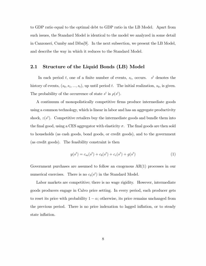
A continuum of monopolistically competitive firms produce intermediate goods

using a common technology, which is linear in labor and has an aggregate productivity

shock, (). Competitive retailers buy the intermediate goods and bundle them into

the final good, using a CES aggregator with elasticity . The final goods are then sold

to households (as cash goods, bond goods, or credit goods), and to the government

(as credit goods). The feasibility constraint is then

() = () + (

) + () + () (1)

Government purchases are assumed to follow an exogenous AR(1) processes in our

numerical exercises. There is no () in the Standard Model.

Labor markets are competitive; there is no wage rigidity. However, intermediate

goods producers engage in Calvo price setting. In every period, each producer gets

to reset its price with probability 1−; otherwise, its price remains unchanged from

the previous period. There is no price indexation to lagged inflation, or to steady

state inflation.

8

The utility of the representative household is

=

∞X=0

X

()£¡¢ ¡¢ ¡¢ ¡¢¤

(2)

=

∞X=0

[ ]

where is hours worked. As these equations suggest, we will suppress the notation

for the state, , when we think that it will cause no confusion.

In period (or more precisely, state ) households may purchase state contingent

securities, (+1), that pay one dollar in state +1 and cost (+1|). Householdscan construct a riskless bond, , by purchasing a portfolio of claims that costs one

dollar and pays a gross rate of return () in every future state +1:

1 = ()X+1|

(+1|) (3)

In our LB Model, there are actually two risk free bonds, and is issued

by the private sector and cannot be used as collateral to purchase bond goods. We

will refer to as the CCAPM rate (for reasons that will become evident in the next

subsection). Since households are identical in our models, there will be no private

sector demand for in equilibrium. However, the government can hold private

sector bonds in the Benchmark LB Model; so, the net demand for these bonds will

be (

), the government’s holding of In the Constrained LB Model, = 0 is

a constraint on government behavior. is the bond issued by the government, and

it pays a gross rate of return . This is the liquid bond that can be used as collateral

in the purchase of bond goods. In the Standard Model, government bonds do not

provide liquidity, and and are perfect substitutes and =

Each period is divided into two exchanges. In the financial exchange, public and

private agents do all of their transacting except for the actual buying and selling

9

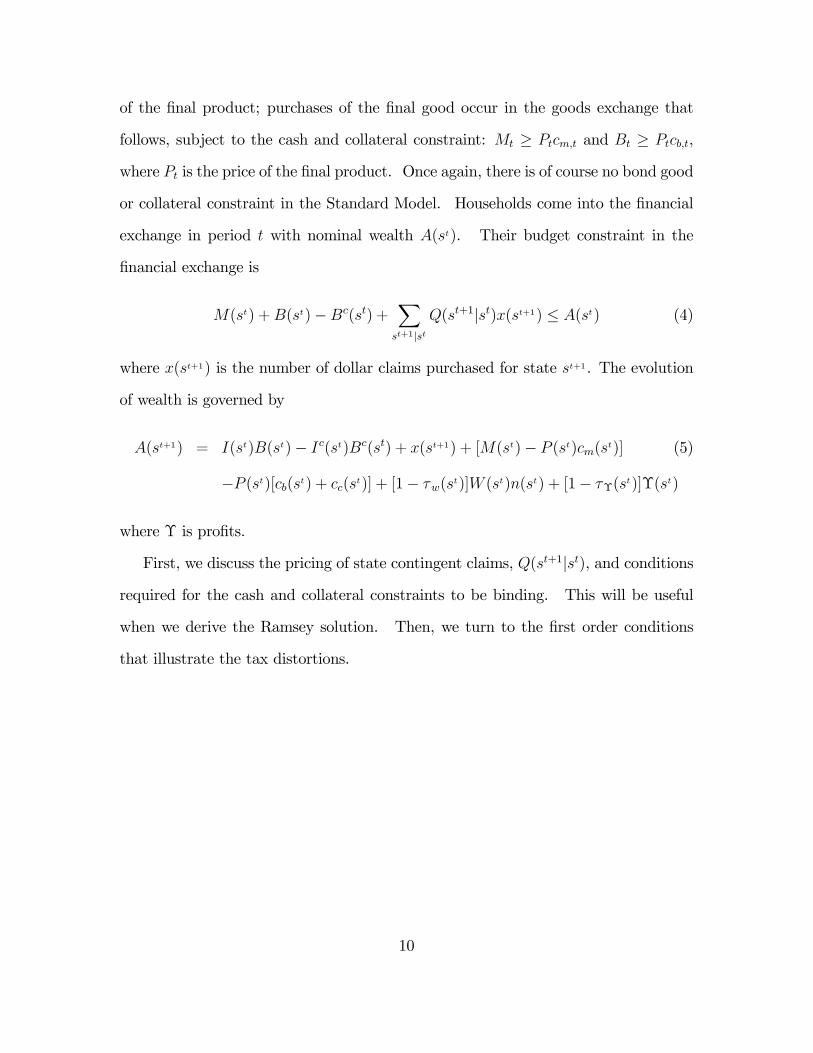
of the final product; purchases of the final good occur in the goods exchange that

follows, subject to the cash and collateral constraint: ≥ and ≥ ,

where is the price of the final product. Once again, there is of course no bond good

or collateral constraint in the Standard Model. Households come into the financial

exchange in period with nominal wealth (). Their budget constraint in the

financial exchange is

() +()−() +X+1|

(+1|)(+1) ≤ () (4)

where (+1) is the number of dollar claims purchased for state +1. The evolution

of wealth is governed by

(+1) = ()()− ()() + (+1) + [()− ()()] (5)

− ()[() + ()] + [1− (

)] ()() + [1− Υ()]Υ()

where Υ is profits.

First, we discuss the pricing of state contingent claims, (+1|), and conditionsrequired for the cash and collateral constraints to be binding. This will be useful

when we derive the Ramsey solution. Then, we turn to the first order conditions

that illustrate the tax distortions.

10

2.2 Pricing of State Contingent Claims

Households maximize

[()] = max{ £ ¡¢ ¡¢ ¡¢ ¡¢¤ (6)

+¡¢[¡¢−

¡¢¡¢]

+¡¢[¡¢−

¡¢¡¢]

+¡¢[()−()−() +()−

X+1|

(+1|)(+1)]

+X+1|

(+1|) [(+1)]}

First order conditions from this maximization give the pricing equation for state

contingent claims

(+1|) = (+1|)∙(

+1)

()

()

(+1)

¸(7)

The first order conditions also imply that ≤ ; this reflects the fact that govern-

ment bonds pay a non-pecuniary return (or yield transactions services). Moreover,

the cash in advance constraint is binding ( () 0) if 1 and the collateral

constraint is binding ( () 0) if .

2.3 Tax Distortions and Euler Equations

The household’s first order conditions imply

= (8)

If the household gives up one dollar’s worth of the cash good, it can spend dollars

on the credit good, because credit goods avoid the cash in advance constraint. Since

the final good can be sold as either a cash good or a credit good, the marginal rate of

transformation is one for one. So if 1, the household buys too few cash goods.

11

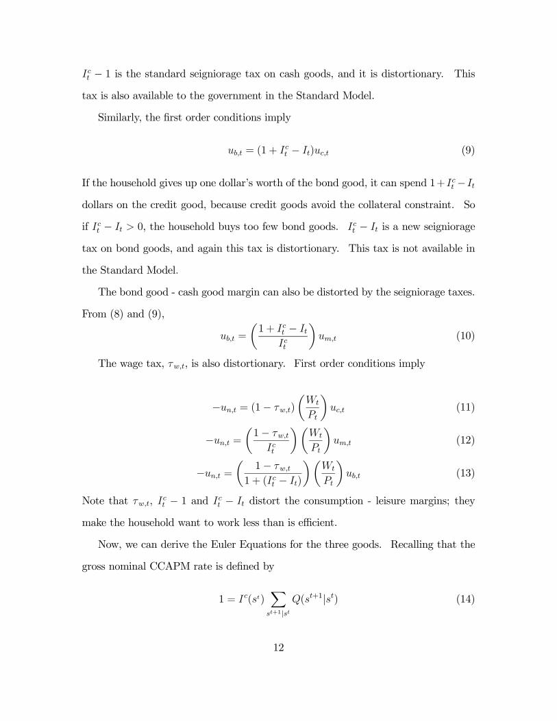
− 1 is the standard seigniorage tax on cash goods, and it is distortionary. This

tax is also available to the government in the Standard Model.

Similarly, the first order conditions imply

= (1 + − ) (9)

If the household gives up one dollar’s worth of the bond good, it can spend 1+ −dollars on the credit good, because credit goods avoid the collateral constraint. So

if − 0, the household buys too few bond goods. − is a new seigniorage

tax on bond goods, and again this tax is distortionary. This tax is not available in

the Standard Model

The bond good - cash good margin can also be distorted by the seigniorage taxes.

From (8) and (9),

=

µ1 + −

¶ (10)

The wage tax, , is also distortionary. First order conditions imply

− = (1− )

µ

¶ (11)

− =µ1−

¶µ

¶ (12)

− =µ

1−

1 + ( − )

¶µ

¶ (13)

Note that , − 1 and − distort the consumption - leisure margins; they

make the household want to work less than is efficient.

Now, we can derive the Euler Equations for the three goods. Recalling that the

gross nominal CCAPM rate is defined by

1 = ()X+1|

(+1|) (14)

12

and using the pricing equation for contingent claims, (7), we arrive at the standard

Euler equation

1 =

∙+1

+1

¸(15)

Then, (8) implies the Euler equation for credit goods

1 =

∙+1

+1

+1

¸(16)

Note that intertemporal smoothing of the credit good depends on next period’s in-

terest rate; that is, +1appears in this Euler equation instead of ; The reason is

that the credit good is not paid for until period + 1 Finally, (9) implies the Euler

Equation for bond goods

1 =

∙+1

µ1 + −

1 + +1 − +1

¶µ+1

+1

¶¸(17)

The difference in the timing of these seigniorage taxes will play a role in the next

section.

2.4 The Government’s Present Value Budget Constraint

So, where does the second seigniorage tax — the one on bonds — show up in the

government’s fiscal accounting? In the LB Model, the consolidated government flow

budget constraint can be written as

+ − + =−1 + −1−1 − −1

−1 (18)

where is the primary surplus, and where it will be recalled that is the govern-

ment’s stock of private sector bonds. Let (≡−1+−1−1−−1−1) be total

government liabilities at the beginning of period . Then, iterating the flow budget

constraint forward, and applying the household transversality condition, yields the

13

present value budget constraint.

=

∞X=0

+

∙+ +

µ+ − 1+

¶µ+

+

¶+

µ+ − +

+

¶µ+

+

¶¸(19)

where + is the stochastic discount factor. The next to last term in the equation

is the standard seigniorage tax. The last term is the seigniorage tax on bonds; it

reflects the fact that the government borrows at a discount, due to the non-pecuniary

return on its bonds. Of course, this last tax is not available in the Standard Model.

3 Optimal Money and Debt Management

We can solve the Ramsey problem analytically for the Benchmark LB Model

with flexible prices, and we will begin with that case. Then, we will discuss the

complications that arise in the Constrained LB Model, where the government does

not have access to a Ricardian debt instrument. And finally, we will relate our results

to those found (by others) in the Standard Model.

With staggered price setting, we can no longer solve the Ramsey problem ana-

lytically. The reason is that, as noted by Schmitt-Grohe and Uribe[26] and others,

price rigidity adds a new state variable, one cannot reduce the sequence of flow im-

plementability constraints to a single present value constraint. However, we can

illustrate the optimal solution using numerical methods. Here, the results are quite

different for the Benchmark LB Model and the Constrained LB Model.

In what follows, we will work with the utility function

( ) = log() + log() + log −1

22 (20)

although our results readily extend to more general preferences. In particular, as

explained in the Appendix, our derivation of the Ramsey solution for the Benchmark

14

LB Model with flexible prices extends to preferences that are homothetic over the

three consumption goods and weakly separable across employment and consumption.

In our numerical exercises, we will also let = = ; this symmetry will make

some of the impulse response functions easier to interpret.

One final note before we begin the derivations: Λ() ≡ () + () − ()

represents net real government liabilities. We will let the Ramsey planner set the

initial values of (0), (0), and (0) subject to a given initial value of Λ(0)

(≥ 0)9 This allows the planner to choose arbitrarily large values of initial gross

liabilities, (0) + (0), in the Benchmark LB Model (the only model for which

() is available). The choice of initial gross liabilities will be important in what

follows.

3.1 The Case of Flexible Prices

We begin with the Benchmark LB Model. We present the full derivation of

the Ramsey Solution in an appendix. In the main text, we present a sketch of the

derivation, give intuition for how the solution works, and illustrate the intuition with

impulse response functions from a numerical example.10

9There are important questions about how we should treat the choice of the initial conditions (or

the price level, given some initial nominal liabilities). However, these issues are well known, and we

have nothing new to contribute.10For our numerical examples, the Calvo parameter, , is set at 0.75 for the case of staggered

price setting. Government spending follws an AR(1) process, with the auto-regressive parameter

set at 0.9. , the CES aggregator for the final good is set equal to 7. The steady state debt to

GDP ratio in the Standard Model is set equal to the optimal steady state debt to GDP ratio in the

Benchmark LB Model.

15

3.1.1 The Benchmark LB Model with Flexible Prices

We follow the usual procedure in solving for the Ramsey problem: we derive

flow implementability conditions by using household first order conditions to elimi-

nate relative prices and tax rates in the household’s flow budget constraints; then,

we choose the quantities of consumption and labor that optimize household utility

subject to the relevant constraints. However, the Ramsey planner will also choose

() and () because we have inequality constraints on the consumption of cash

and bond goods. The Ramsey planner will also choose its holdings of private sector

debt, () As we shall see, the flow implementability conditions reduce to a single

present value condition if this Ricardian debt instrument is available to the planner.

The first step is to derive the flow implementability conditions, and incorporate

the complimentary slackness conditions into them. As shown in the appendix, the

household’s flow budget constraint can be written as

() =X+1|

[(+1|)(+1)] +()

∙1− 1

()

¸+()

∙1− ()

()

¸(21)

+ ()

()[(

) + () + (

)]−∙1− ()

()

¸ ()()

The cash in advance constraint is binding for () 1, and we have () = 1 if

this constraint is not binding. So for all () ≥ 1, we have

()

∙1− 1

()

¸= ()(

)

∙1− 1

()

¸(22)

or, rearranging terms,

()

∙1− 1

()

¸+

()()

()= ()(

) (23)

Similarly, the collateral constraint is binding if () (), and we have () =

() if this constraint is not binding. So, for all values of () satisfying 1 ≤ ()

16

≤ (), we have

()

∙1− ()

()

¸= ()(

)

∙1− ()

()

¸= ()(

)

∙()− ()

()

¸(24)

or, rearranging terms,

()

∙1− ()

()

¸+

()()

()= ()(

)

∙1 + ()− ()

()

¸(25)

Substituting the complimentary slackness conditions — (23) and (25) — into (21), and

using household first order conditions to eliminate relative prices and (+1|) wearrive at the flow implementability conditions

()

()()=

X+1|

(+1|)∙

(+1)

(+1)(+1)

¸+ 1− £()¤2 (26)

The Ramsey planner maximizes household utility subject to (26), the feasibility

constraint

() + (

) + () + () = ()() (27)

and the inequality constraints for cash and bond goods. We have put the com-

plementary slackness conditions into the implementability conditions, they are valid

whether or not the constraints are binding. So, all we have left are the inequality

constraints themselves.

As shown in the appendix, two of the first order conditions for this maximization

problem are

(+1)− () = (+1)(

+1)

(28)

and

() = () ( ≡ ()) (29)

where () and () are the Lagrange multipliers for the inequality constraints on

the cash and bond goods, and () is the Lagrange multiplier on the implementability

conditions (26).

17

The cash and collateral constraints are both binding, or they are both slack. If

they are binding (() 0), then (28) says that the Ramsey planner issues more

liabilities, easing the constraints but increasing the tax burden and (+1). If the

inequality constraints are never binding (() = 0), then () = a constant over

time and across states. In this case, we can iterate the flow implementability condi-

tions to obtain a single present value condition. If however the cash and collateral

constraints are binding, then () increases over time, and the flow constraints do

not collapse into a present value constraint.

So, are the cash and collateral constraints binding in the Benchmark LB Model,

or are they not? We have made no mention of the Ramsey planner’s use of its

Ricardian debt instrument, () It turns out that the derivative with respect to

this instrument implies

() = 0 (30)

and therefor () = . We will give a fuller explanation of the role played by the

Ricardian debt instrument later in the section.

As shown in the appendix, the Ramsey planner’s first order conditions for con-

sumption imply

()

=

()=

()

(31)

when () = 0 And since the implementation of the optimal allocation is subject

to household first order conditions (8) and (9), we must have

() = () = 1 (32)

So, the Ramsey planner follows an Extended Friedman Rule: the cost of holding

money is eliminated (() − 1 = 0), and the cost of holding government bonds is

eliminated (() − () = 0). We have satiation in both money and government

18

debt. And of course, () = 1 implies that prices are expected to deflate at the

real rate of interest.

The wage tax is the third distortionary tax. As shown in the appendix, the

optimal tax rate is positive.

() = 1−

µ1

1 + 2()

¶µ

− 1¶ 0 (33)

And since () = , the optimal wage tax rate is constant. The wage tax distortion

is perfectly smoothed over time and across states. Why is the wage tax rate positive

while the the two seigniorage taxes are set to zero? As seen in section 2.3, any of

these taxes would distort the labor - leisure margin. However, using either of the

seigniorage taxes would also distort the relative consumption margins. The wage tax

does not distort the consumption margins; so it is efficient to use it to tax work.11

But if the wage and seigniorage tax rates are held constant, how does the Ram-

sey planner accommodate shocks that have fiscal consequences? Figure 1 illustrates

the Ramsey planner’s response to an auto-corellated increase in government spend-

ing.12 The planner engineers a surprise (shock dependent) inflation; this is a non-

distortionary tax that lowers the real value of government liabilities, or equivalently

households’ real assets. Households respond by decreasing consumption and increas-

ing their work effort to rebuild their wealth. The three goods are perfect substitutes

in production, and they enter utility in an identical way. So, their consumption

paths are identical, declining by equal amounts and then returning to their steady

state values at equal rates. A rising path of consumption requires a real interest rate

that is above its steady state value. The nominal interest rate enters the three Euler

equations — (15), (16) and (17) — in different ways, and the Extended Friedman Rule

11Chari et al[11] relate this result to Atkinson and Stiglitz[5].12We use numerical methods for illustration only. We provide an analytical derivation of the

Ramsey solution in the Appendix.

19

(() = () = 1) nullifies these differences. The required movements in the real

interest rate are accomplished by expected inflation.

Since all of the tax rates are unchanged, the persistent increase in government

purchases results in a deficit. The Ramsey planner finances the deficit by issuing

new liabilities, and this is of course what allows the households to rebuild their wealth.

But what if the initial inflation tax on money and bonds makes the cash and

collateral constraints binding? This would distort consumption patterns and raise

interest rates, none of which happens. Here is where () comes in. Recall

that we have let the Ramsey planner set the initial values of its liabilities, (0)

and (0), subject to a given (possibly zero) initial value of net liabilities, Λ(0) =

(0) + (0) − (0) By lending to the private sector, the planner can build up

(0) and (0) to a level where the cash and collateral constraint will be never

binding. This debt instrument, unlike government bonds, is Ricardian; its supply

has no direct effect on household consumption decisions.

3.1.2 The Constrained LB Model with Flexible Prices

In the Constrained LB Model, the government is not allowed to hold private

sector debt; that is, () ≡ 0 The government does not have a Ricardian debt

instrument. The steady state solution and all of the first order conditions for this

problem are the same as in the Benchmark case except of course for the condition

with respect to () which made (

) constant and kept the cash and collateral

constraints from binding. If initial liabilities are small, then the cash and collateral

constraints will bind for large shocks. In this case, (28) implies that the government

will issue more liabilities going into states with binding inequality constraints (recall

that a rising shadow price corresponds to higher public-sector liabilities). We will

assume that initial liabilities are large enough for the inequality constraints not to

20

bind. In this case the Ramsey solution coincides with the solution when we let the

government buy private bonds.

3.1.3 The Standard Model with Flexible Prices

In the Standard Model, there is no bond good and no collateral constraint. As

Chari, Christiano and Kehoe[11] have shown, the original Friedman Rule is optimal in

the Standard Model with flexible prices.13 There is no need for government lending,

() here. Public debt, () is a Ricardian instrument. It can be issued to finance

temporary deficits. And if, say, the response to an increase in government spending

requires an initial inflation tax that would make the cash constraint binding, then

the Ramsey planner can use open market operations to change the composition of

total liabilities and avoid the problem.

Surprise inflation is quite volatile in Chari, Christiano and Kehoe’s numerical

simulations. In their benchmark calibration, inflation has a standard deviation of

20 percent per annum. This price volatility can also be seen in Figure 1 for the

Benchmark LB Model.

3.2 The Case of Staggered Price Setting

With flexible prices, we saw that the Friedman Rule was optimal and the ex-

pected rate of deflation was equal to the real rate of interest; moreover, the Ramsey

Planner made substantial use of unanticipated inflation to absorb the fiscal conse-

quences of macroeconomic shocks. This is costless when prices are flexible. But, as

is well known, staggered price setting can create a dispersion of intermediate goods’

prices that distorts household consumption decisions.14 And if (as we assume) prices

13Canzoneri, Cumby and Diba[9] provide a fuller discussion the earlier literature.14Woodford[30] is the classic reference.

21

are not indexed to inflation, there can also be a dispersion of prices in the steady

state. This relative price distortion can be eliminated if the Ramsey Planner fixes

the price level; in this case, price setters will not want to change their prices even

when given the opportunity.

So, staggered price setting creates a fundamental inflation tradeoff for the Ramsey

Planner. Fixing the price level to eliminate the price dispersion clashes with the

implementation of the Friedman Rule, and with the use of unanticipated inflation as a

fiscal shock absorber. The question becomes: how important is the distortion created

by the price dispersion relative to the distortions created by the seigniorage taxes

and the wage tax? Benigno and Wooford[7] and Schmitt-Grohe and Uribe[26], using

calibrated models similar to our Standard Model, found that the inflation tradeoff

was basically resolved in favor of price stability.

As noted above, we can not solve the Ramsey problem analytically with staggered

price setting. So, we have to resort to numerical methods.15 We will begin with

a discussion of optimal taxation and inflation in the various models’ steady states.

Then, we will show how the Ramsey planner responds to an unexpected increase in

government spending. We will begin with the Standard Model, since the planner’s

response reflects the conventional wisdom that grew out of the work of Barro. Then,

we will proceed to the Benchmark LB Model, which retains the basic insights of

Barro. Finally, we will discus the Constrained LB Model, in which the government

does not have available a Ricardian debt instrument and the insights of Barro are

lost.

15More precisely, we use the Get Ramsey program developed by Levin and Lopez-Salido[21] and

Levin, Otnatski, Williams, and Williams[22].

22

3.2.1 Optimal Tax Rates and Inflation in the Steady State

Table 1 reports optimal steady state tax rates and inflation for our numerical

calibrations of the various models. With flexible prices, the seigniorage taxes are set

to zero and the wage and profit taxes service the public debt; deflation is equal to

the real rate of interest. With staggered price setting, prices are virtually fixed, and

the seigniorage taxes are positive. Calvo trumps Friedman: the inflation tradeoff is

resolved decidedly in favor of price stability.

Table 1 shows that 1 Why is this? If were set equal to 1, (10) implies

that the bond good - cash good margin would not be distorted, but (9) implies that

the bond good - credit good margin would be distorted. Similarly setting =

would leave the bond good - credit good margin undistorted, but the bond good - cash

good margin would be distorted. Optimal policy spreads the consumption distortions

by setting 1 Moreover, the cash seigniorage tax is larger than the bond

seigniorage tax. This must be the case, since 1 implies that − 1 − 16

3.2.2 Optimal Responses in the Standard Model

Figure 2 shows the Ramsey planner’s response to an auto-corellated increase in

government spending, and it reflects the conventional wisdom. As before, households

respond to the increased tax burden by decreasing consumption and working more.

Here however, there is virtually no unanticipated inflation; it is just too costly in

terms of the price dispersion it creates. The spending increase has to be financed

another way.

Raising the seigniorage tax, or the wage tax, , creates a distortion, and the

Ramsey planner minimizes these distortions by issuing liabilities to finance part of

16With the symmetry in our utility function, is set exactly half way between zero and

23

the increase in government spending. This leaves a larger public debt to be rolled

over in the new steady state, and the wage tax is raised permanently to finance that.

In this way, the Ramsey planner trades off short run tax smoothing against lower

long run consumption. This tradeoff, and the unit root it engenders, captures the

fundamental insight of Barro.

The consumption paths of the cash good and the credit good are very similar after

the first few periods, and they resemble the consumption paths for the flexible price

case. As before, the optimal allocation requires that consumption falls initially and

then rises over time, requiring that the real interest rate be above its steady state

value. Now, however, the nominal interest rate needs to change because inflation is

too costly to move. And as a result, the paths of cash and credit good consumption

are similar, but not identical.

The Ramsey planner takes some artful steps in the first few periods to smooth

initial distortions. The need for these steps arises because of the difference in the

timing of the interest rates in Euler equations (15) and (16). From (16), a drop

in period 1 credit good consumption requires an increase in 2, the nominal interest

rate in period 2. But this will distort the relative consumption of cash and credit

goods in period 2; that is, cash good consumption will be too low. To mitigate the

cost of this, the planner makes cash good consumption fall by less than credit good

consumption in period 1, which requires a decrease in 1.

In order to achieve the optimal paths of consumption, the Ramsey planner has to

alter the composition of government liabilities so that household money balances are

consistent with cash good consumption. Since public debt is Ricardian, open market

sales of bonds allow the cash in advance constraint to be satisfied with no further

consequences.

The details of the artful steps taken by the Ramsey planner in the first few periods

24

depend on the special timing in the cash and credit good apparatus. They may not

be robust to changes in the way of modeling liquidity. The important result here is

that optimal policy involves short run tax smoothing and permanent effects on debt,

consumption, and the wage tax rate.

3.2.3 Optimal Responses in the Benchmark LB Model

Figure 3 shows the Ramsey planner’s response to a persistent increase in gov-

ernment spending, and it is similar to that in Figure 2. In particular, Barro’s

fundamental insight survives: short run tax distortions are smoothed at the expense

of longer run consumption. There is, however, a twist in the Ramsey planner’s im-

plementation of the policy due to the fact that government bonds are now used as

collateral; they are no longer Ricardian. Government assets, are Ricardian, and

they play an important role in what follows; we return to this issue at the end of the

section.

As before, the increase in government spending crowds out consumption and in-

creases work effort in the short run, and once again the three consumption goods’

paths are very similar after the first few periods. Inflation (not pictured) is too costly

to move. So, the real interest rate increases, associated with the rising consumption

profiles, require changes in the seigniorage taxes, − 1 and − . Consequently,

the consumption paths are not identical.

As with the standard model, the Ramsey planner takes some complicated steps

in the first few periods. The increase in 2 again implies that period 2 cash good

consumption will fall too much relative to credit good consumption, and this loss

is mitigated by a decrease in 1. But the divergence in period 1 cash and credit

good consumption has a utility cost. The Ramsey planner must choose bond good

consumption in a way that mitigates that utility cost while achieving a drop in over-

25

all period 1 consumption large enough to accommodate the increase in government

purchases. This is achieved by balancing the smaller drop in cash good consumption

with a larger drop in bond good consumption; that is, the decline in credit good

consumption is between these two.

The difference in bond and credit good consumption must be reflected in the

interest rate spread, − . From (17), the interest rate entering the Euler equation

for the bond good is +1+1

, which differs from that in the Euler equation for

the credit good by the spread terms. If the spread were to remain constant at its

steady state value, the response of bond good consumption would be identical to that

of credit good consumption. But since bond good consumption falls by more than

credit good consumption and is therefore expected to rise by more, the real interest

rate for bond goods must be higher and the spread must be expected to fall. And

since the spread returns to its steady state value, a declining spread implies an initial

increase in the spread.

Now, we return to the role played by The Ramsey planner cannot simply alter

the composition of government liabilities to achieve the optimal allocation: satisfying

the cash in advance constraint requires selling government bonds. But in the LB

Model, this would loosen the collateral constraint, and too many bond goods would

be consumed. The government can finance its short run deficit in the normal way

(by issuing more total liabilities), but then the government sells for and . In

this way, the cash and collateral constraints can be made consistent with optimal

allocation of cash and bond good consumption.

3.2.4 Optimal Responses in the Constrained LB Model

Figure 4 shows the Ramsey planner’s response to a sustained increase in gov-

ernment spending, and it clearly violates the conventional wisdom. The Ramsey

26

solution is stationary; the government does not smooth short run tax distortions at

the expense of longer run consumption.

The reason is that both money and government bonds provide liquidity in the LB

Model, and the path of consumption is tied to their supplies. Without a Ricardian

debt instrument (like in the Standard Model or in the Benchmark LBModel), the

planner cannot finance temporary surpluses or deficits without affecting the supply of

liquidity to households. Stated differently, without the Ricardian instrument, fiscal

policy and liquidity provision cannot be determined independently.

Consumption is again crowded out by the increase in government purchases. The

decline in cash and bond good consumption requires a corresponding decline in both

and . (This means of course that the government has to run a surplus.) Comparing

Figures 3 and 4, the Ramsey planner has to raise the wage tax more by a full order

of magnitude. And this means that consumption has to fall by about twice as much

and the additional work effort is curtailed.

The Ramsey planner’s steps in the first few periods are even more artful than

in the previous cases. Private sector holdings of nominal government liabilities are

inherited from the previous period and real liabilities will initially change only as a

result of inflation. Since inflation is small, the sum of the change in and — and

therefore the sum of the changes in cash and bond good consumptions — is close to

zero. But since interest rates must change to reflect the optimal consumption paths,

the ratio of consumption of the cash and bond goods must change. If the sum of the

changes is nearly zero and the ratio changes, one must rise and one must fall. From

above, we know that it is cash good consumption that will rise because 1 can be used

to mitigate the distortion resulting from an increase in 2. In order to mitigate the

utility cost of differing consumption of the 3 goods, bond good consumption will fall

less than credit good consumption. (If it were to fall by more, cash good consumption

27

would need to rise by even more.) In addition, to mitigate the effect of this distortion,

inflation while negligible is much greater here than in the previous case.

Because the decline of credit good consumption exceeds the decline of bond good

consumption, expected growth of credit good consumption exceeds expected growth

of bond good consumption. Therefore the interest rate in the credit good Euler

equation exceeds that in the bond good Euler equation. The spread is therefore

expected to grow and must therefore decline initially.

3.2.5 The Benefit of having a Government Lending Instrument

Figure 5 compares the Ramsey planner’s responses to an increase in government

spending in three models: the Benchmark LB Model with flexible prices, the Bench-

mark LB Model with staggered price setting, and the Constrained LB Model with

staggered price setting. The figure illustrates the potential benefit of the govern-

ment’s having a Ricardian debt instrument like

Staggered price setting adds a nominal distortion to the model. But when is

available, the consumption paths are quite similar to those with flexible prices. When

is not available, consumption of all three goods falls much further. Of course, long

run consumption is a little lower when is used.

In contrast, the response of government liabilities to a spending shock is much

smaller when the Ramsey planner does not have access to a Ricardian debt instru-

ment. This stands in sharp contrast to the much greater response seen for consump-

tion and the wage tax rate. The reason is, once again, that tax policy and liquidity

provision cannot be determined independently without a Ricardian debt instrument.

The liquidity value of government liabilities introduces a motive for the Ramsey plan-

ner to smooth debt as well as the labor tax rate. Alternatively, the Ramsey planner

needs to trade off smoothing the wage tax rate and smoothing the bond seigniorage

28

tax rates. That trade-off is resolved in this model by a much greater wage tax rate

volatility.

4 Conclusion

In this paper, we asked how the fundamental insights of Friedman and Barro

fare when we recognize the fact that bonds provide liquidity services. To investigate

this question, we augmented a standard cash and credit good model by allowing

government bonds to be used as collateral in purchasing certain types of consumption

goods. In this environment, the government cannot use its bonds to finance a short

run deficit (ala Barro) independently of its decision of how much liquidity to provide

for consumption. We found that the insights of Friedman and Barro survive largely

intact if the government has at its disposal an additional debt instrument that is

“Ricardian” — in the sense that it does not directly affect economic activity. Absent

a Ricardian debt instrument, the Friedman Rule may not be optimal in the transition

to a steady state, even with flexible prices. And with sticky prices, the Ramsey

planner would no longer choose to smooth short run tax distortions at the expense

of some long run consumption (ala Barro).

We model the Ricardian debt instrument as government holdings of private sector

bonds, which by our assumptions did not provide liquidity services. But, it would

not seem that governments currently utilize a Ricardian debt instrument. They

certainly do not use private sector debt in the way our Ramsey planner would. They

do of course have non-liquid assets such as parks, oil rights, grazing rights, spectrum

rights, and state owned enterprises. However these assets would be hard to use to

finance short run deficits without creating disruptions in the real economy.

Finally, future research might usefully focus on relaxing some of the sharp distinc-

29

tions that we have made in our modeling of money and bond liquidity. For example,

some kinds of private debt may well compete with government bonds in the provision

of liquidity services. Such debt would not qualify as a Ricardian debt instrument for

use in the manner described here. A more elaborate modeling of the use of various

financial assets would seem to be warranted. In a similar vein, long term government

debt may not provide the liquidity services envisioned in our model. If this is the

case, then long term government bonds may qualify as the Ricardian debt instru-

ment that is needed here. Modeling a term structure of debt may help differentiate

the financial assets that do and do not provide liquidity. More generally yet, the

substitutability between money and bonds in the provision of liquidity could be ex-

plored further. This could be done by say increasing the substitutability of the cash

and bond goods in utility. As the cash and bond goods became perfect substitutes,

money would presumably be crowed out. Or alternatively, holding the elasticity of

substitution constant, one could explore the implications of the central bank’s paying

interest on reserves. This could lead to a discussion of the optimal approach to a

winding down of the "unconventional policies" pursued by central banks in recent

years.

5 Appendix: Ramsey Solution to the LB Model

with Flexible Prices

We can solve the Ramsey problem analytically for the LB Model with flexible

prices. In the Benchmark LB Model, the government is able to lend to the private

sector; that is, is a policy instrument. In the Constrained LB Model is not

available.

30

We follow the usual procedure in solving for the Ramsey solution: we derive flow

implementability conditions by using household first order conditions to eliminate

relative prices and tax rates from the household’s flow budget constraints; then,

we choose the quantities of consumption and labor that optimize household utility

subject to the relevant constraints. However, the Ramsey Planner will also choose

() and () because we have inequality constraints on the consumption of cash

and bond goods. We have to insert complementary slackness conditions into the

implementability conditions to allow for the possibility that these constraints are

not binding in the optimal solution. Finally, the Ramsey planner will also choose

its holdings of private sector debt, () As we shall see, the flow implementability

conditions reduce to a single present value condition if this Ricardian debt instrument

is available to the planner.

One final note before we begin the derivations: there are important questions

about how we should treat the choice of the initial government liabilities (or the price

level, given some initial nominal liabilities). However, these issues are well known,

and we have nothing new to contribute. In the benchmark model, we will let the

Ramsey planner set the initial values (0), (0), and (0), subject to a given

(possibly zero) value of net liabilities, (0) + (0) − (0) We will return to the

question of where the planner would set these initial values later in the appendix.

We begin by deriving the flow implementability constraint. Assuming non-

satiation in some state, the household budget constraint, (4), holds with equality;

using (5) to eliminate (+1), we get

() = () +() +() +X+1|

(+1|) {(+1)

−()− ()()− ()()

+ ()[() + (

) + ()]− [1− (

)] ()()} (34)

31

We have set after tax profits to zero because profits are pure monopoly rents in

our model, and we know that the Ramsey planner will tax them away. UsingP+1| (

+1|) = 1()

the budget constraint becomes

() =X+1|

[(+1|)(+1)] +()

∙1− 1

()

¸+()

∙1− ()

()

¸(35)

+ ()

()[(

) + () + (

)]−∙1− ()

()

¸ ()()

Next, we incorporate the complementary slackness conditions for the cash and

collateral constraints. The cash in advance constraint is binding for () 1, and

we have () = 1 if this constraint is not binding. So for all () ≥ 1, we have

()

∙1− 1

()

¸= ()(

)

∙1− 1

()

¸(36)

or

()

∙1− 1

()

¸+

()()

()= ()(

) (37)

Similarly, the collateral constraint is binding if () (), and we have () =

() if this constraint is not binding. So, for all values of () satisfying 1 ≤ ()

≤ (), we have

()

∙1− ()

()

¸= ()(

)

∙1− ()

()

¸= ()(

)

∙()− ()

()

¸(38)

or

()

∙1− ()

()

¸+

()()

()= ()(

)

∙1 + ()− ()

()

¸(39)

Substituting (37) and (39) into (35), the budget constraint becomes

() =X+1|

[(+1|)(+1)] + ()

½(

) +() + ()

()(40)

+

∙()− ()

()

¸(

)

¾−∙1− ()

()

¸ ()()

32

Next, we use the household’s first order conditions (8), (9), and (12) to eliminate

relative prices and tax rates,

() =X+1|

[(+1|)(+1)] + ()

½(

) +()()

()(41)

+()()

()+

()()

()

¾And using (7), we get

()()

()=

X+1|

(+1|)∙(+1)(+1)

(+1)

¸+ (

)() (42)

+()(

) + ()(

) + ()()

Equation (42) is a series of implementibility constraints, one for each period and

state, . With flexible prices, in the Standard Model the flow constraints can be

reduced to a single present value constraint beginning in 0 See Canzoneri, Cumby

and Diba ([9]) This is also true in the LB Model if is available. However, if is

not available, the cash and collateral constraints can be binding and we have to work

with the flow implementibility constraints, even with flexible prices.

We should also note that there are implementability constraints implied by 1 ≤() ≤ () (see equations (9) and (10)),

() ≤ (

) ≤ () (43)

We will tentatively ignore these constraints and leave them to be verified later.

To lighten our exposition, we will work with the utility function

log() + log() + log −1

22 (44)

although our results readily extend to preferences that are homothetic over the three

consumption goods and weakly separable across employment and consumption, as in

33

Chari, et. al.[11][12].17 With this specification of preferences, the implementability

constraints (42) simplify to

()

()()=

X+1|

(+1|)∙

(+1)

(+1)(+1)

¸+ 1− £()¤2 (45)

The Ramsey planner maximizes household utility subject to (45), the feasibility

constraint

() + (

) + () + () = ()() (46)

and the inequality constraints for cash and bond goods. We have already put the

complementary slackness conditions into the implementability constraints; they are

valid whether or not these constraints are binding. So, all we have left are the

inequality constraints themselves,

() ≤ () (47)

and

() ≤ () (48)

We can now solve the planner’s problem. Let () denote the left hand side of

the implementability constraint,

() ≡ ()

()()=

£() + ()− (

)¤

()(49)

Let () denote the Lagrange multipliers for the implementability constraints, and

incorporate these constraints in the Lagrange function as

()()

⎧⎨⎩X+1|

(+1|)(+1) + 1− £()¤2 − ()

⎫⎬⎭ (50)

17We don’t present these derivations because they mimic very closely the derivations in Chari et.

al.[12]

34

Let () denote the multipliers for the feasibility condition, (46), and incorporate

these constraints in the Lagrange function as

()()£()()− (

)− ()− (

)− ()¤

(51)

Finally, let () and () be the multipliers for the inequality constraints, and

(since = − − ) incorporate them in the Lagrange function as

()

⎧⎪⎨⎪⎩ ()h()()

− ()− (

)− ()i

+() [()− ()]

⎫⎪⎬⎪⎭ (52)

We begin with the first order conditions for consumption and work effort:

The FOC for () gives

()

= () (53)

The FOC for () gives

()

= () + () (54)

The FOC for () gives

()

= () + ()

∙1− ()

¸(55)

or

()

= () +()

()[(

)−()] (56)

And, the FOC for () gives

£1 + 2()

¤() = ()() (57)

Next, we have the first order conditions for the financial variables:

The FOC for (+1) gives

()()(+1|)−+1(+1)(+1)++1(+1)(+1)(

+1)

= 0 (58)

35

We have ()(+1|) = (+1) or else (+1|) = 0 because +1 is just the

history followed by the realization +1 of the random variables at date + 1. So,

this FOC reduces to

(+1)− () = (+1)(

+1)

(59)

This equation says that the shadow price of the implementability constraint is increas-

ing over time if the inequality constraint for cash goods is binding.

The FOC for () gives

() = () ≡ () (60)

We also have the non-negativity conditions with the complementary slackness condi-

tions

()£()− (

)] = ()[()− ()¤= 0 (61)

In the Benchmark LB Model, the government is allowed to buy household debt;

that is, it has another policy instrument, () In this case, the Ramsey solution sim-

plifies quite dramatically:

The FOC for () gives

() = 0

Then, (59) implies that (0) = () ≡ for all states and dates; the series of

implementibility constraints can be iterated forward to obtain a single present value

implementability constraint.

More importantly, the inequality constraints on cash and bond holdings will never

bind if the government can buy private debt. And this is why the Lagrange multi-

pliers, (), are constant. The Ramsey planner does not have to use () to finance

fiscal imbalances, which could be distortionary. The Constrained LB Model does not

share these features.

36

When () = 0 the FOC’s for consumption imply

()

=

()=

()

= () (62)

Since the optimal allocation satisfies (62), and its implementation is subject to (8)

and (9), we have

() = () = 1

The extended Friedman Rule is optimal. This also confirms that (43) is satisfied.

Using (62) and (57), the Ramsey allocation satisfies

(1 + 2)()() = (

) (63)

Since the implementation of optimal policy is subject to (12), with the real wage

equal to ( − 1)(), (63) and () = 1 imply

(1 + 2)[1− () ] =

− 1

and a constant optimal tax rate

() = 1−

µ1

1 + 2

¶µ

− 1¶

(64)

To calculate optimal allocations, we need to pin down the value of . Using (46),

(62) and (63), we get

(1 + 2) ( − ) =

which implies

=1

2

⎡⎣ +s()

2+()

2

1 + 2

⎤⎦ (65)

Iterating (45), we get

0

0= 0

+∞X=0

©1− []2

ª

37

which, together with (55) and (57), implies

0(1 + 2)0

0= 0

+∞X=0

©1− []2

ªSubstituting (65) and taking expectations will pin down

References

[1] Aiyagari, S. Rao, Albert Marcet, Thomas Sargent, and Juha Seppala, 2002, "Op-

timal Taxation without State-Contingent Debt," Journal of Political Economy,

University of Chicago Press, vol. 110(6), December, 1220-1254.

[2] Aiyagari, S. Rao, and Ellen McGrattan, 1998, "The optimum quantity of debt,"

Journal of Monetary Economics, 42, 447-469.

[3] Albanesi, Stefania, 2003, “Comments on "Optimal Monetary and Fiscal Policy:

A Linear-Quadratic Approach" by Pierpaolo Benigno and Michael Woodford, in

Mark Gertler and Kenneth Rogoff (eds.), NBER Macroeconomics Annual 2003.

[4] Angeletos, George-Marios, Fabrice Collard, Harris Dellas, and Behzad Diba,

2012, "Public Debt as Optimal Liquidity Provision," mimeo.

[5] Atkinson, Anthony, and Joseph Stiglitz, 1976, "The design of tax structure:

Direct versus indirect taxation," Journal of Public Economics, vol. 6(1-2), 55-

75.

[6] Barro, Robert, 1979, "On the Determination of the Public Debt," The Journal

of Political Economy, Vol. 87, No. 5, Part 1, pp. 940-971.

38

[7] Benigno, Pierpaolo and Michael Woodford, 2003,“Optimal Monetary and Fiscal

Policy: A Linear-Quadratic Approach,” in Mark Gertler and Kenneth Rogoff

(eds.), NBER Macroeconomics Annual.

[8] Bensal, Ravi, John Coleman, 1996, “A Monetary Explanation of the Equity

Premium, Term Premium, and Risk-Free Rate Puzzles,” Journal of Political

Economy, No 6, 1135-1171.

[9] Canzoneri, Matthew, Robert Cumby and Behzad Diba, 2011, “The Interaction

Between Monetary and Fiscal Policy” in Handbook of Monetary Economics, Vol.

3, Benjamin Friedman and Michael Woodford editors, Elsevier.

[10] Calvo, Guillermo and Carlos Végh, 1995, “Fighting inflation with high interest

rates: the small open economy case under flexible prices,” Journal of Money

Credit and Banking, v. 27 no. 1, 49-66.

[11] Chari, V., Lawrence Christiano and Patrick Kehoe, 1991, "Optimal Fiscal and

Monetary Policy: Some Recent Results," Journal of Money, Credit and Banking,

Ohio State University Press, vol. 23(3), pages 519-39, August.

[12] __________, 1996, "Optimality of the Friedman Rule in Economies with

Distorting Taxes," Journal of Monetary Economics, Vol. 37, 202-223.

[13] Correia, Isabel, Juan Nicolini and Pedro Teles, 2008, “Optimal Fiscal and Mon-

etary Policy: Equivalence Results,” Journal of Political Economy, 168, 1, pp.

141-170.

[14] Defiore, Fiorella, and Pedro Teles, 2003, "The Optimal Mix of Taxes on Money,

Consumption and Income," Journal of Monetary Economics, Vol. 50, 871-887.

39

[15] Friedman, Benjamin, and Kenneth N. Kuttner, 1998, "Indicator Properties Of

The Paper-Bill Spread: Lessons From Recent Experience," The Review of Eco-

nomics and Statistics, MIT Press, vol. 80(1), pages 34-44, February.

[16] Friedman, Milton, 1969, The Optimum Quantity of Money and Other Essays,

Aldine Publishing Company, Chicago.

[17] Greenwood, Robin, and Dimitri Vayanos, 2010, “Bond Supply and Excess Bond

Returns,” NBER Working Paper Series No. 13806.

[18] Holmström, Bengt and Jean Tirole, 1998, "Private and Public Supply of Liquid-

ity", 1998, The Journal of Political Economy, Vol. 106, No. 1 (February 1998),

pp. 1-40.

[19] Hu, Yifan, and Timothy Kam, 2009, "Bonds with transactions service and opti-

mal Ramsey policy", Journal of Macroeconomics, Volume 31, Issue 4, December,

Pages 633-653.

[20] Krishnamurthy, Arvind, and Annette Vissing-Jorgensen, 2012, “The Aggregate

Demand for Treasury Debt”, Journal of Political Economy, Vol. 12, No. 2, pp

233-267.

[21] Levin, Andrew, and David Lopez-Salido, 2004, “Optimal Monetary Policy with

Endogenous Capital Accumulation”, unpublished manuscript, Federal Reserve

Board.

[22] Levin, Andrew, Alexei Onatski, John C. Williams, and Noah Williams, 2005,

“Monetary Policy Under Uncertainty in Micro-Founded Macroeconometric Mod-

els,” in Mark Gertler and Kenneth Rogoff (eds.), NBER Macroeconomics Annual

2005, Cambridge, MIT Press, pp. 229-287.

40

[23] Linnemann, Ludger and Andreas Schabert, 2010, “Debt Nonneutrality, Policy

Interactions, And Macroeconomic Stability," International Economic Review,

vol. 51(2), pages 461-474.

[24] Patinkin, Don, 1965, Money, Interest, and Prices: An Integration of Monetary

and Value Theory, 2nd edition, (Harper & Row, New York).

[25] Pflueger, Carolin and Luis Viceira, 2011, “An Empirical Decomposition of Risk

and Liquidity in Nominal and Inflation Indexed Government Bonds”, NBER

Working Paper #16892, March.

[26] Schmitt-Grohe, Stephanie, and Martin Uribe, 2004, “Optimal Fiscal and Mon-

etary Policy under Sticky Prices,” Journal of Economic Theory, 114, February,

pg. 198-230.

[27] Schmitt-Grohe, Stephanie, and Martin Uribe, 2005, “Optimal Fiscal and Mon-

etary Policy in a Medium-Scale Macroeconomic Model,” in Mark Gertler and

Kenneth Rogoff (eds.), NBER Macroeconomics Annual, Cambridge, MIT Press,

pp. 383-425.

[28] Woodford, Michael, 1990a, “The Optimum Quantity of Money,” in B.M. Fried-

man and F.H. Hahn eds., Handbook of Monetary Economics, Volume II, Ams-

terdam, Elsevier Science, pp. 1067-1152.

[29] Woodford, Michael, 1990b, "Public Debt as Private Liquidity," American Eco-

nomic Review, Vol. 80, No. 2, Papers and Proceedings, pp. 382 - 388.

[30] Woodford, Michael, 2003, Interest and Prices: Foundations of a Theory of Mon-

etary Policy, Princeton University Press, Princeton.

41

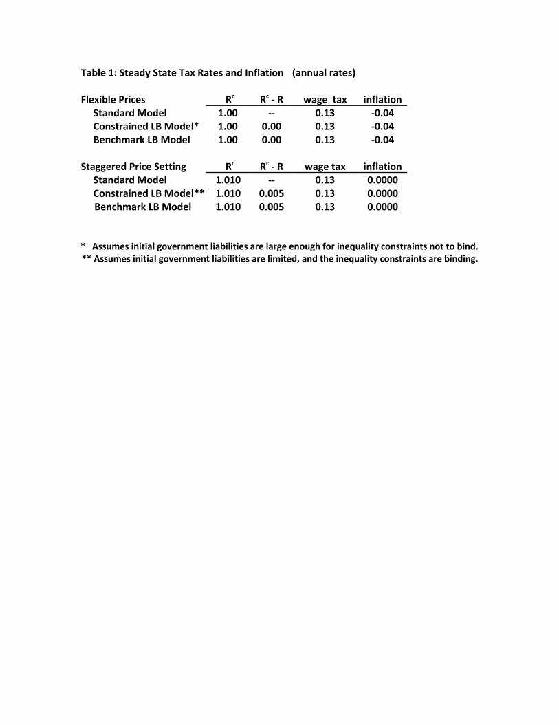
Table 1: Steady State Tax Rates and Inflation  (annual rates)

Flexible Prices         Rc Rc ‐ R wage  tax inflation     Standard Model      1.00 ‐‐ 0.13 ‐0.04     Constrained LB Model*      1.00 0.00 0.13 ‐0.04     Benchmark LB Model      1.00 0.00 0.13 ‐0.04

Staggered Price Setting         Rc Rc ‐ R wage tax inflation     Standard Model     1.010 ‐‐ 0.13 0.0000     Constrained LB Model**     1.010 0.005 0.13 0.0000  Benchmark LB Model     1.010 0.005 0.13 0.0000

       *   Assumes initial government liabilities are large enough for inequality constraints not to bind.       ** Assumes initial government liabilities are limited, and the inequality constraints are binding.

10 20 30 40-1.5

-1

-0.5

0x 10

-3 cash good consumption

10 20 30 400

0.5

1

1.5x 10

-3 work

10 20 30 40-1.5

-1

-0.5

0x 10

-3 bond good consumption

10 20 30 40-0.02

0

0.02

0.04

0.06inflation

10 20 30 40-1.5

-1

-0.5

0x 10

-3 credit good consumption

10 20 30 400

1

2

3x 10

-3 deficit

Figure 1: Benchmark LB Model with flexible prices, government spending shock

10 20 30 40-2

-1.5

-1

-0.5

0x 10

-3 cash good

10 20 30 40-2

-1.5

-1

-0.5

0x 10

-3 credit good

10 20 30 40-5

0

5

10

15x 10

-4 work

10 20 30 40-1

0

1

2

3x 10

-6 inflation

10 20 30 40-2

-1

0

1

2x 10

-4 I

10 20 30 400

1

2

3

x 10-4 wage tax rate

10 20 30 400

0.02

0.04

0.06

0.08

government liabilities

10 20 30 400

0.02

0.04

0.06

0.08

government bonds

Figure 2: Standard Model, staggered price setting

10 20 30 40-2

-1.5

-1

-0.5

0x 10

-3 cash good

10 20 30 40-2

-1.5

-1

-0.5

0x 10

-3 bond good

10 20 30 40-2

-1.5

-1

-0.5

0x 10

-3 credit good

10 20 30 40-5

0

5

10

15x 10

-4 work

10 20 30 40-6

-4

-2

0

2x 10

-4 I

10 20 30 400

0.5

1

1.5x 10

-4 Ic - I

10 20 30 400

1

2

3

x 10-4 wage tax rate

10 20 30 400

0.01

0.02

0.03

0.04

net government liabilities

10 20 30 40-0.02

-0.015

-0.01

-0.005

0government assets

Figure 3: Benchmark LG, staggered price setting

10 20 30 40

-4

-2

0

2x 10

-3 cash good

10 20 30 40-3

-2

-1

0x 10

-3 bond good

10 20 30 40-5

-4

-3

-2

-1

0x 10

-3 credit good

10 20 30 40-5

0

5

10

15x 10

-4 work

10 20 30 40-2

0

2

4x 10

-5 inflation

10 20 30 40

-4

-2

0

2

x 10-3 I

10 20 30 40-2

-1.5

-1

-0.5

0x 10

-3 Ic - I

10 20 30 400

1

2

3

x 10-3 wage tax rate

10 20 30 40-2

-1.5

-1

-0.5

0x 10

-3 government liabilities

Figure 4: Constrained LB Model, staggered price setting

10 20 30 40

-4

-2

0

2

x 10-3 cash good

10 20 30 40-3

-2.5

-2

-1.5

-1

-0.5

0x 10

-3 bond good

10 20 30 40-5

-4

-3

-2

-1

0x 10

-3 credit good

10 20 30 40-5

0

5

10

15x 10

-4 work

Figure 5: Comparison of responses in the LB models

Note: solid line = Benchmark LB Model (flexible prices); dashed line = Benchmark LB Model (staggered price setting); dotted line = Constrained LB Model (staggered price setting).