Optimal Inapproximability Results for MAX-CUTand Other 2-Variable CSPs?

Subhash Khot∗

College of ComputingGeorgia Tech

khot@cc.gatech.edu

Guy Kindler†

Theory GroupMicrosoft Research

gkindler@microsoft.com

Elchanan Mossel‡

Department of StatisticsU.C. Berkeley

mossel@stat.berkeley.edu

Ryan O’Donnell∗

Theory GroupMicrosoft Research

odonnell@microsoft.com

September 19, 2005

Abstract

In this paper we show a reduction from the Unique Games problem to the problem of approximatingMAX-CUT to within a factor of αGW + ε, for all ε > 0; here αGW ≈ .878567 denotes the approxima-tion ratio achieved by the Goemans-Williamson algorithm [25]. This implies that if the Unique GamesConjecture of Khot [36] holds then the Goemans-Williamson approximation algorithm is optimal. Ourresult indicates that the geometric nature of the Goemans-Williamson algorithm might be intrinsic to theMAX-CUT problem.

Our reduction relies on a theorem we call Majority Is Stablest. This was introduced as a conjecturein the original version of this paper, and was subsequently confirmed in [42]. A stronger version ofthis conjecture called Plurality Is Stablest is still open, although [42] contains a proof of an asymptoticversion of it.

Our techniques extend to several other two-variable constraint satisfaction problems. In particular,subject to the Unique Games Conjecture, we show tight or nearly tight hardness results for MAX-2SAT,MAX-q-CUT, and MAX-2LIN(q).

For MAX-2SAT we show approximation hardness up to a factor of roughly .943. This nearly matchesthe .940 approximation algorithm of Lewin, Livnat, and Zwick [40]. Furthermore, we show that our.943... factor is actually tight for a slightly restricted version of MAX-2SAT. For MAX-q-CUT we showa hardness factor which asymptotically (for large q) matches the approximation factor achieved by Friezeand Jerrum [24], namely 1 − 1/q + 2(ln q)/q2.

For MAX-2LIN(q) we show hardness of distinguishing between instances which are (1−ε)-satisfiableand those which are not even, roughly, (q−ε/2)-satisfiable. These parameters almost match those achievedby the recent algorithm of Charikar, Makarychev, and Makarychev [10]. The hardness result holds evenfor instances in which all equations are of the form xi − xj = c. At a more qualitative level, this resultalso implies that 1 − ε vs. ε hardness for MAX-2LIN(q) is equivalent to the Unique Games Conjecture.

∗Work performed while the author was at the Institute for Advanced Study. This material is based upon work supported by theNational Science Foundation under agreement Nos. DMS-0111298 and CCR-0324906 respectively. Any opinions, findings andconclusions or recommendations expressed in this material are those of the authors and do not necessarily reflect the views of theNational Science Foundation.

†Work performed while the author was at DIMACS and at the Institute for Advanced Study, Princeton, and was partly supportedby CCR grant NCCR-0324906 and NDMS-0111298.

‡Supported by a Miller fellowship in Computer Science and Statistics, U.C. Berkeley

Electronic Colloquium on Computational Complexity, Report No. 101 (2005)

ISSN 1433-8092

1 Introduction

The main result in this paper is a bound on the approximability of the MAX-CUT problem which matchesthe approximation ratio achieved by the well-known Goemans-Williamson algorithm [25]. The proof of thishardness result relies on the Unique Games Conjecture of Khot [36]. We also rely critically on a theoremwe call Majority Is Stablest, which was introduced as a conjecture in the original version of this paper. Forthe convenience of the reader we will now briefly describe these two tools; formal statements appear inSections 3 and 4.

Unique Games Conjecture (roughly): Given a bipartite graph G, a large constant size set of labels [M ],and a permutation of [M ] written on each edge, consider the problem of trying to find a labeling of thevertices of G from [M ] so that each edge permutation is ‘satisfied.’ The conjecture is that if M is a largeenough constant then it is NP-hard to distinguish instances which are 99% satisfiable from instances whichare 1% satisfiable.

Majority Is Stablest Theorem (roughly): Let f be a boolean function which is equally often 0 or 1.Suppose the string x is picked uniformly at random and the string y is formed by flipping each bit of xindependently with probability η; we call Pr[f(x) = f(y)] the noise stability of f . The theorem statesthat among all f in which each coordinate has o(1) ‘influence,’ the Majority function has the highest noisestability, up to an additive o(1).

We add in passing that the name Majority Is Stablest is a bit of a misnomer in that almost all bal-anced boolean threshold functions are equally noise stable (see Theorem 5). We also note that the MajorityIs Stablest theorem has interesting applications outside of this work — to the economic theory of socialchoice [33] for example — and may well prove useful for other PCP-based inapproximability results. InSection 6.3 we mention interesting generalizations of the Majority Is Stablest theorem for q-ary functions,q > 2, which are relevant for hardness of approximation and are not resolved in full.

Despite the fact that our hardness result for MAX-CUT relies on the unproven Unique Games Conjec-ture, we feel it is interesting for several reasons. First, in our opinion it is remarkable that the Unique GamesConjecture should yield a tight hardness of approximation ratio for MAX-CUT, and that indeed the bestfactor should be the peculiar number αGW. It is intriguing that the precise quantity αGW should arise from anoise stability property of the Majority function, and certainly there was previously little evidence to suggestthat the Goemans-Williamson algorithm might be optimal.

Another reason we believe our result is interesting is related to this last point. Since the Goemans-Williamson algorithm was published a decade ago there has been no algorithmic progress on approximatingMAX-CUT. Since Hastad’s classic inapproximability paper [31] from two years later there has been noprogress on the hardness of approximating MAX-CUT, except for the creation of a better reduction gad-get [51]. As one of the most natural and simple problems to have resisted matching approximability bounds,we feel MAX-CUT deserves further investigation and analysis. In particular, we think that regardless ofthe truth of the Unique Games Conjecture, this paper gives interesting insight into the geometric natureof MAX-CUT. Indeed, insights we have gleaned from studying the MAX-CUT problem in this light havemotivated us to give new positive approximation algorithms for variants of other 2-variable CSPs such asMAX-2SAT; see Section 9.

Finally, instead of viewing our result as relying on the unproven Unique Games Conjecture, we canview it as being an investigation into the truth of UGC. Indeed our hardness results for both MAX-CUTand for two-variable linear equations modulo q provide explicit parameters for which the Unique GamesConjecture, if true, must hold. (Note that both problems are Unique Games themselves.) Thus our workgives a target for algorithmic attacks on the Unique Games Conjecture, which if passed will refute it.

2

Indeed, works subsequent to the original version of this paper have provided approximation algorithmsfor the Unique Games problem [50, 28, 10] improving on Khot’s original algorithm [36]. In particular,in [10] Charikar, Makarychev, and Makarychev gave a semidefinite programming-based approximationalgorithm for Unique Games whose approximation factor nearly matches our hardness bound for MAX-2LIN(q). The current situation is therefore that any improvement in the approximation factors for eitherMAX-CUT or for the more general MAX-2LIN(q) will refute the Unique Games Conjecture.

1.1 Overview of the paper

In Section 2 we describe the MAX-CUT problem and discuss its history. We then state the Unique GamesConjecture in Section 3 and discuss very recent algorithm results for the problem. The Majority Is Stablestproblem is discussed in Section 4, along with its generalization to q-ary domains, q ≥ 2. We discuss thegeometric aspects of MAX-CUT and their connection with Majority Is Stablest result and the Goemans-Williamson approximation algorithm in Section 5. Our main results are stated in Section 6. Section 7 isdevoted to some technical definitions, preliminaries, and Fourier analytic formulas. In Section 8 we proveour main theorem on the hardness of approximating MAX-CUT, based on the Unique Games Conjecture.In Section 9 we investigate the approximability of other binary 2-CSPs, such as MAX-2SAT. Finally, Sec-tion 11 is devoted to extending our techniques to the q-ary domain; we prove some results about noisestability in this domain and then prove our Unique Games-hardness results for MAX-q-CUT and MAX-2LIN(q) and MAX-q-CUT.

2 About MAX-CUT

The MAX-CUT problem is a classic and simple combinatorial optimization problem: Given a graph G, findthe size of the largest cut in G. By a cut we mean a partition of the vertices of G into two sets; the size of thecut is the number of edges with one vertex on either side of the partition. One can also consider a weightedversion of the problem in which each edge is assigned a nonnegative weight and the goal is to cut as muchweight as possible.

MAX-CUT is NP-complete (indeed, it is one of Karp’s original NP-complete problems [35]) and soit is of interest to try to find polynomial time approximation algorithms. For maximization problems suchas MAX-CUT we say an algorithm gives an α-approximation if it always returns an answer which is atleast α times the optimal value; we also often relax this definition to allow randomized algorithms whichin expectation give α-approximations. Crescenzi, Silvestri, and Trevisan [11] have shown that the weightedand unweighted versions of MAX-CUT have equal optimal approximation factors (up to an additive o(1))and so we pass freely between the two problems in this paper.

The trivial randomized algorithm for MAX-CUT — put each vertex on either side of the partition in-dependently with equal probability — is a 1/2-approximation, and this algorithm is easy to derandom-ize; Sahni and Gonzalez [45] gave the first 1/2-approximation algorithm in 1976. Following this some(1/2 + o(1))-approximation algorithms were given, but no real progress was made until the breakthrough1994 paper of Goemans and Williamson [25]. This remarkable work used semidefinite programming toachieve an αGW-approximation algorithm, where the constant αGW ≈ .878567 is the trigonometric quantity

αGW = min0<θ<π

θ/π

(1 − cos θ)/2.

The optimal choice of θ is the solution of θ = tan(θ/2), namely θ∗ ≈ 2.33 ≈ 134, and αGW = 2π sin θ∗ .

The geometric nature of Goemans and Williamson’s algorithm might be considered surprising, but as weshall see, this geometry seems to be an inherent part of the MAX-CUT problem.

3

On the hardness of approximation side, MAX-CUT was proved MAX-SNP hard [44] and Bellare, Gol-dreich, and Sudan [2] explicitly showed that it was NP-hard to approximate MAX-CUT to any factor higherthan 83/84. The hardness factor was improved to 16/17 ≈ .941176 by Hastad [31] via a reduction fromMAX-3LIN using a gadget of Trevisan, Sorkin, Sudan, and Williamson [51]. This stands as the current besthardness result.

Despite much effort and many improvements in the approximation guarantees of other semidefinite pro-gramming based algorithms, no one has been able to improve on the algorithm of Goemans and Williamson.Although the true approximation ratio of Goemans-Williamson was proved to be not more than αGW [34, 18]and the integrality gap of their semidefinite relaxation was also proved to be αGW [18], there appears on theface of it to be plenty of possibilities for improvement. Adding triangle constraints and other valid con-straints to the semidefinite program has been suggested, alternate rounding schemes have been proposed,and local modification heuristics that work for special graphs have been proven (see, e.g., [25, 17, 16, 34,52, 15, 18]). And of course, perhaps a completely different algorithm altogether can perform better. Sev-eral papers have either explicitly ([16]) or implicitly ([18]) given the problem of improving on αGW as animportant research goal.

However, in this paper we show that approximating MAX-CUT to within any factor larger than αGW willin fact overturn the Unique Games Conjecture.

3 About the Unique Games Conjecture

MAX-CUT belongs to the class of constraint satisfaction problems on 2 variables (2-CSPs). In a k-CSP weare given a set of variables and a set of constraints, where each constraint depends on exactly k variables.The goal is to find an assignment to the variables so as to maximize the number of constraints satisfied. Inthe case of MAX-CUT, the vertices serve as variables and the edges as constraints. Every constraint saysthat two certain variables should receive different boolean values.

Proving inapproximability results for a k-CSP is equivalent to constructing a k-query PCP with a specificacceptance predicate. Usually the so-called Label Cover problem is a starting point for any PCP construc-tion. Label Cover is a 2-CSP where the variables range over a large (non-boolean) domain. Usually, inap-proximability results for boolean CSPs are obtained by encoding assignments to Label Cover variables viaa binary code and then running PCP tests on the (supposed) encodings. This approach has been immenselysuccessful in proving inapproximability results for k-CSPs with k ≥ 3 (see for example [31, 46, 29]). How-ever the approach gets stuck in the case of 2-CSPs. We seem to have no techniques for constructing boolean2-query PCPs and the bottleneck seems to be the lack of an appropriate PCP ‘outer verifier.’

Khot suggested the Unique Games Conjecture in [36] as a possible direction for proving inapproxima-bility results for some important 2-CSPs, such as Min-2SAT-Deletion, Vertex Cover, Graph-Min-Bisectionand MAX-CUT. This conjecture asserts the hardness of the ‘Unique Label Cover’ problem:

Definition 1. The Unique Label Cover problem, L(V,W,E, [M ], πv,w(v,w)∈E) is defined as follows:Given is a bipartite graph with left side vertices V , right side vertices W , and a set of edges E. The goalis to assign one ‘label’ to every vertex of the graph, where [M ] is the set of allowed labels. The labeling issupposed to satisfy certain constraints given by bijective maps σv,w : [M ] → [M ]. There is one such mapfor every edge (v, w) ∈ E. A labeling ‘satisfies’ an edge (v, w) if

σv,w(label(w)) = label(v).

The optimum OPT of the unique label cover problem is defined to be the maximum fraction of edges satisfiedby any labeling.

4

The Unique Label Cover problem is a special case of the Label Cover problem. It can also be statedin terms of 2-Prover-1-Round Games, but the Label Cover formulation is easier to work with. The UniqueGames Conjecture asserts that this problem is hard:

Unique Games Conjecture: For any η, γ > 0, there exists a constant M = M(η, γ) such that it is NP-hardto distinguish whether the Unique Label Cover problem with label set of size M has optimum at least 1 − ηor at most γ.

The Unique Games Conjectures asserts the existence of a powerful outer verifier that makes only 2queries (albeit over a large alphabet) and has a very specific acceptance predicate: for every answer to thefirst query, there is exactly one answer to the second query for which the verifier would accept, and viceversa. Once we have such a powerful outer verifier, we can possibly construct a suitable inner verifier andprove the desired inapproximability results. Typically, though, the inner verifier will need to rely on ratherdeep theorems about the Fourier spectrum of boolean functions, e.g. the theorem of Bourgain [7] or ofFriedgut [21].

The Unique Games Conjecture was used in [36] to show that Min-2SAT-Deletion is NP-hard to ap-proximate within any constant factor. The inner verifier is based on a test proposed by Hastad [30] and onBourgain’s theorem. It is also implicit in this paper that the Unique Games Conjecture with an additional‘expansion-like’ condition on the underlying bipartite graph of the Label Cover problem would imply thatGraph-Min-Bisection is NP-hard to approximate within any constant factor. Khot and Regev [37] showedthat the conjecture implies that Vertex Cover is NP-hard to approximate within any factor less than 2. The in-ner verifier in their paper is based on Friedgut’s theorem and is inspired by the work of Dinur and Safra [14]that showed 1.36 hardness for Vertex Cover. In the present paper we continue this line of research, showingan inner verifier that together with the Unique Games Conjecture yields a tight hardness result for MAX-CUT. Our inner verifier relies critically on the Majority Is Stablest theorem.

Algorithmic results for Unique Label Cover. It is natural to ask how the function M(η, γ) in the UniqueGames Conjecture can behave. Lower bounds on M are obtained by giving algorithms for Unique LabelCover. Several very recent results have provided such algorithms. Most relevant for this paper is the algo-rithm of [10], which has the following behavior for Unique Label instances with label set of size q: For anyconstant η > 0, on instances with optimum 1− η it satisfies roughly a (1/q)η/(2−3η) fraction of edges, up tolower order powers of q. Also, for η = 1/ log q, it seems to satisfy an Ω(1) fraction of edges (at the presenttime the final version of [10] has not yet appeared).

4 About the Majority Is Stablest problem

To state the Majority Is Stablest problem, we need some definitions. For convenience we regard the booleanvalues as −1 and 1 rather than 0 and 1. Thus a boolean function is a map f : −1, 1n → −1, 1. We willoften generalize to the case of functions f : −1, 1n → R. In all of what follows we consider the set ofstrings −1, 1n to be a probability space under the uniform distribution.

First we recall the well-known notion of ‘influence’, introduced to computer science in [3] and studiedeven earlier in economics.

Definition 2. Let f : −1, 1n → R. Then the influence of xi on f is defined by

Infi(f) = E(x1,...,xi−1,xi+1,...,xn)

[Varxi[f ]] .

5

(Note that for f : −1, 1n → −1, 1,

Infi(f) = Prx∈−1,1n

[f(x) 6= f(x1, . . . ,−xi, . . . xn)].)

Instead of picking x at random, flipping one bit, and seeing if this changes the value of f , we can insteadflip a constant fraction (in expectation) of the bits. This leads to the study of ‘noise sensitivity,’ pioneered incomputer science by [32, 31, 4].

Definition 3. Let f : −1, 1n → R and let −1 ≤ ρ ≤ 1. The noise stability of f at ρ is defined as follows:Let x be a uniformly random string in −1, 1n and let y be a ‘ρ-correlated’ copy; i.e., pick each bit yi

independently so that E[xiyi] = ρ. Then the noise stability is defined to be

Sρ(f) = Ex,y[f(x)f(y)].

(Note that for f : −1, 1n → −1, 1 we have Sρ(f) = 2Prx,y[f(x) = f(y)] − 1.)

We may now state the Majority Is Stablest theorem. This result was presented as a strongly-believed con-jecture in the original version of this paper. It has recently been proved in [42]. Informally, the theorem saysthat among all balanced boolean functions with small influences, the Majority function has the highest noisestability. Note that the assumption of small influences is necessary since the ‘dictator’ function f(x) = x i

provably has the highest noise stability among all balanced boolean functions, for every ρ. Note that when ntends to infinity, the noise stability at ρ of the n-bit Majority function approaches (1− 2

π arccos ρ) (this factwas stated in a paper of Gulibaud from the 1960’s [27] and is ultimately derived from the Central Limit theo-rem plus a result from an 1890’s paper of Sheppard [47]). Thus we have the formal statement of the theorem:

Majority Is Stablest theorem: Fix ρ ∈ [0, 1). Then for any ε > 0 there is a small enough δ = δ(ε, ρ) > 0such that if f : −1, 1n → [−1, 1] is any function satisfying E[f ] = 0 and Inf i(f) ≤ δ for all i = 1 . . . n,then

Sρ(f) ≤ 1 − 2π arccos ρ + ε.

In the remainder of this section, we shall describe why the Majority Is Stablest theorem is relevant forMAX-CUT inner verifiers.

As described in the previous section, inapproximability results for many problems are obtained by con-structing a tailor-made PCP; usually, the PCP is obtained by composing an ‘outer verifier’ (almost alwaysa Label Cover problem) with an ‘inner verifier’. As mentioned the outer verifier for our reduction is theUnique Label Cover problem. As for the inner verifier, it is always application-specific and its acceptancepredicate is tailor-made for the problem at hand, in our case MAX-CUT.

A codeword test is an essential submodule of an inner verifier. It is a probabilistic procedure for checkingwhether a given string is a codeword of an error-correcting code, most commonly the ‘Long Code’ (see [2]).

Definition 4. The Long Code over domain [n] is a binary code in which the message space is in fact the setof truth tables of boolean functions f : −1, 1n → −1, 1. The codeword encoding the ‘message’ i ∈ [n]is given by the ith dictator function; i.e., the function f(x1, x2, . . . , xn) = xi.

A codeword test for the Long Code can often be extended to a full-fledged inner verifier. So in thefollowing, we will focus only on a Long Code test. The choice of the test is determined by the problem athand, in our case MAX-CUT. The test must read two bits from a Long Code and accept if and only if thevalues read are distinct. Note that a legal Long Code word, i.e. a dictator, is the truth table of a boolean

6

function in which one coordinate has influence 1. Let us say that a function f is far from being a LongCode if all the coordinates have o(1) influences (note that this is not a standard notion of being far from acodeword, but rather a notion tailored for our proof technique).

We expect the following from a codeword test: a correct Long Code word passes the test with probabilityc (called the ‘completeness’ parameter of the test) whereas any function far from being a Long Code passesthe test with probability at most s (called the ‘soundness’ parameter). Once we construct a full-fledged innerverifier, the ratio s/c will be the inapproximability factor for MAX-CUT.

The Long Code test. As mentioned before, our Long Code test will need to take a boolean functionf : −1, 1n → −1, 1, pick two inputs x and y, and check that f(x) 6= f(y). In fact our test will beprecisely a ‘noise stability’ test for some fixed noise rate ρ; i.e., x will be chosen uniformly at random andy will be formed by flipping each bit of x independently with probability 1

2 − 12ρ. Here ρ will be a value

between −1 and 0, and therefore y is a highly noisy version of x, or alternatively, a moderately noisy versionof −x. Thus (at least for legal Long Code words) we expect f(x) to be quite anticorrelated with f(y); i.e.,it should pass the test with relatively high probability. Recalling Definition 3, we see that the probability agiven function f passes our test is precisely 1

2 − 12Sρ(f).

A legal Long Code word, i.e. a dictator function, has noise stability precisely ρ and thus the completenessof the Long Code test is c = 1

2− 12ρ. The crucial aspect of our test is the analysis of the soundness parameter.

This is where the Majority Is Stablest theorem comes in. Suppose f : −1, 1n → −1, 1 is anyfunction that is far from being a Long Code word. By a simple trick (see Proposition 7.4) we can show thatthe Majority Is Stablest theorem (which is stated only for ρ ≥ 0) implies that for ρ < 0 the noise stability off at ρ is at least 1 − 2

π arccos ρ (a negative number). Hence it follows that functions that are far from beinga Long Code pass the test with probability at most s = 1

2 − 12(1 − 2

π arccos ρ) = (arccos ρ)/π.Choosing ρ < 0 as we please, this leads to an inapproximability ratio of

s

c= min

−1<ρ<0

(arccos ρ)/π12 − 1

2ρ= min

0≤θ≤π

θ/π

(1 − cos θ)/2= αGW,

precisely the Goemans-Williamson constant.

4.1 History of the Majority Is Stablest problem

There has been a long line of work in the analysis of boolean functions studying the noise sensitivityof functions and the associated Fourier-theoretic quantities (some examples, roughly in chronological or-der: [32, 8, 48, 22, 49, 9, 21, 4, 6, 7, 23, 33, 41, 43, 13]). Building on the intuition gathered from this pastwork, we were motivated to make the Majority Is Stablest conjecture in the originial version of the paper.We discuss these relevant previous results below.

The Majority and weighted majority (or balanced threshold) functions have always played an importantrole in the study of noise sensitivity of boolean functions. This family of functions is, in a sense, the set of all“uniformly noise-stable” functions. In [4], it is shown that a family of monotone functions is asymptoticallynoise sensitive if and only if it is asymptotically orthogonal to the family of balanced threshold functions;by asymptotically noise sensitive functions it is meant those that have Sρ(f) = o(1) for any constant ρ.

Stated in terms of Fourier coefficients (see Section 7.2), the Majority Is Stablest theorem says that amongall ‘non-junta-like’ functions, the one which has most Fourier mass on the lower levels is the Majorityfunction. This is because Sρ(f) is a just a weighted sum of the squared Fourier coefficients of f , wherecoefficients at level k have weight ρk. Some strong evidence in favor of the Majority Is Stablest theoremwas given by Bourgain [7], who showed that non-junta functions f have their Fourier tails

∑|S|>k f(S)2

7

lower-bounded by k−1/2−o(1) . As Bourgain noted, the Majority function has precisely this tail decay andthus his theorem is ‘basically’ optimal. In other words, Majority has the ‘least’ Fourier weight on higherlevels and therefore the ‘most’ Fourier weight on lower levels.

The expression S−1/3(f) played a central role in a Fourier-theoretic approach to the Condorcet Paradoxand Arrow’s Theorem given by Kalai [33]. This expression determines the probability of an “irrational out-come” in a certain voting scheme. Much of [33] is devoted to the study of S−1/3(f) and in particular, it isconjectured there (Conjecture 5.1) that for ‘transitive’ functions, which have the property that all influencesare the same, the sum

∑|S|≤k f(S)2 is maximized by the Majority function for all k. Although this conjec-

ture turns out to be false, the corollaries of the conjecture in [33] are implied by the fact that Majority is thestablest transitive function, and this is a consequence of the Majority Is Stablest theorem.

Finally, in [43] it was shown that Majority is essentially the maximizer for another noise stability prob-lem, namely maximizing the kth norm of Tρf , where Tρ is the Bonami-Beckner operator (see Section 7)among balanced functions f for large k and n = ∞.

For some interesting special cases of the Majority Is Stablest theorem we can give short and simpleproofs. These are shown in Section 10.

4.2 Generalizations to the q-ary domain

Our methods can also be used to obtain hardness results for constraint satisfaction problems over variablesranging over larger domains [q]. In the q-ary regime we need a multi-valued analogue of the Majority IsStablest theorem. Before we can formulate the appropriate analogue, we need to specify what we mean by‘q-ary functions’ and also to define the notions of noise stability and influences for them.

The obvious generalization of a boolean function to the q-ary regime would be a function of the formf : [q]n → [q]. However, as we did for boolean functions, we will consider a continuous relaxation of therange. Specifically, define

∆q = (x1, . . . , xq) ∈ [0, 1]q :∑

xi = 1,which can be thought of as the space of probability distributions over [q]. We will consider functionsf : [q]n → ∆q; this generalizes functions f : [q]n → [q] if we identify the elements a ∈ [q] in f ’s rangewith the points (0, . . . , 0, 1, 0, . . . , 0) ∈ ∆q.

Definition 5. Let − 1q−1 ≤ ρ ≤ 1 and let x and y be [q]n-valued random variables. We say that x and y are

a ρ-correlated pair if x is uniformly distributed on [q]n, and y is formed from x by choosing each yi so thatPr[yi = a] = δxi=aρ + 1−ρ

q for each a, independently for each i. Note that for 0 ≤ ρ ≤ 1, it is equivalentto say that each coordinate yi is independently chosen to be xi with probability ρ and is a uniformly randomelement of [q] otherwise.

Definition 6. Let f : [q]n → ∆q and let − 1q−1 ≤ ρ ≤ 1. The noise stability of f at ρ is defined to be

Sρ(f) = Ex,y

[〈f(x), f(y)〉],

where x and y are a ρ-correlated pair. Equivalently, we may define the noise stability of functions g : [q]n →R via

Sρ(g) = Ex,y

[g(x)g(y)]

and then denoting by f i the ith coordinate projection of f , we have Sρ(f) =∑n

i=1 Sρ(fi).

We remark that when f ’s range is simply [q] (as embedded in ∆q), the quantity Sρ(f) is simply theprobability that f(x) = f(y) when x and y are a ρ-correlated pair.

The definition of influences is very similar to that in the boolean case:

8

Definition 7. Let f : [q]n → ∆q. For 1 ≤ i ≤ n, the influence of the ith coordinate on f is defined to be

Infi(f) = Ex1,...,xi−1,xi+1,...,xn

[Varxi[f i(x1, . . . , xn)]].

We say that f : [q]n → ∆q is ‘balanced’ if E[f i] = 1/q for each i. The most obvious generalizationof the Majority function to the q-ary domain is the Plurality function, which on input x ∈ [q]n outputs themost common value for xi (tie-breaking is unimportant). It is natural to ask whether a “Plurality Is Stablest”theorem holds. This question is still open, and we present it as a conjecture. For this purpose, define

PlurStab(q, ρ) = limn→∞

Sρ(Pluralityn,q).

The limit in the formula above indeed exists, and there appears to be no closed formula for it; however weprovide an exact description of it in Theorem 8 in Section 6.

Plurality Is Stablest Conjecture. Fix q ≥ 2 and − 1q−1 ≤ ρ ≤ 1. Then for any ε > 0 there is a small

enough δ = δ(ε, ρ, q) such that if f : [q]n → [q] is any balanced q-ary function with Inf i(f) ≤ δ for alli = 1 . . . n, then

Sρ(f) ≤ PlurStab(q, ρ) + ε

Note that in the case q = 2, Sheppard’s formula gives PlurStab(2, ρ) = 1 − 2π arccos ρ, which is the

noise stability of Majority; there is also a closed formula for q = 3 ([26, 12]). For large values of q we giveasymptotics which hold up to a 1 + oq(1) factor in Section 6. For the reader’s convenience, we remark herethat

PlurStab(q, ρ) = Θ((1/q)(1−ρ)/(1+ρ)

).

Although we don’t have Plurality Is Stablest, a result of [42] generalizing Majority Is Stablest servesus almost equally well. This result bounds the stability of a function in terms of the behavior of correlatedGaussians. To state it, we need one more definition:

Definition 8. Let µ ∈ [0, 1] and ρ ∈ [0, 1]. Let X and Y denote normal random variables with mean 0 and

covariance matrix(

1 ρρ 1

). We define

Λρ(µ) = Pr[X ≥ t and Y ≥ t],

where t is chosen so that Pr[X ≥ t] = µ.

MOO theorem: Fix q ≥ 2 and ρ ∈ [0, 1). Then for any ε > 0 there is a small enough δ = δ(ε, ρ, q) > 0such that if f : [q]n → [0, 1] is any function satisfying E[f ] = µ and Inf i(f) ≤ δ for all i = 1 . . . n, then

Sρ(f) ≤ Λρ(µ) + ε.

As a result we have that the noise stability of any balanced f : [q]n → ∆q is essentially at mostqΛρ(1/q). We give the asymptotics of this quantity in Section 6 and they are extremely close to those ofPlurStabρ(q); in particular, they are the same up to a constant multiplicative factor.

9

5 On the geometry of MAX-CUT

We shall now try to explain (non-rigorously) the connection between the Majority Is Stablest theorem and thegeometric picture that arises from the Goemans-Williamson algorithm. But before going further, let us firstnote that the approximation ratio achieved by Goemans-Williamson arises as the solution of a trigonometricminimization problem, which in turn originates from a geometric setting. To obtain a matching inapprox-imability constant, it seems essential to introduce some similar geometric structure. Such a structure ispresent in the construction of our Long Code test, although it is only implicit in the actual proofs.

For the purposes of the following explanation, let us consider the n-dimensional discrete cube −1, 1n

as a subset of the n-dimensional Euclidean unit sphere (we normalize the Euclidean norm accordingly). TheMajority Is Stablest theorem essentially states that the discrete cube is a good approximation of the spherein a certain sense.

The Goemans-Williamson algorithm. We start with a brief description of how the approximation ratioαGW arises in the Goemans-Williamson algorithm. To find a large cut in a given graph G = (V,E) with nvertices, the Goemans-Williamson algorithm embeds the graph in the unit sphere of Rn, identifying eachvertex v ∈ V with a unit vector xv on the sphere. The embedding is selected such that the sum

∑

(u,v)∈E

1

2− 1

2〈xu,xv〉, (1)

involving the inner products of vectors associated with the endpoints of edges of G, is maximized. Themaximum sum bounds from above the size of the maximum cut, since the size of every cut can be realizedby associating all the vertices from one side of the cut with an arbitrary point x on the sphere, and associatingall other vertices with −x.

Once the embedding is set, a cut in G is obtained by choosing a random hyperplane through the originand partitioning the vertices according to the side of the hyperplane on which their associated vectors fall.For an edge (u, v) in G, the probability that u and v lie on opposite sides of the random cut is proportionalto the angle between xu and xv . More precisely, letting ρ = 〈xu,xv〉 denote the inner product between thevectors associated with u and v, the probability that the edge (u, v) is cut is (arccos ρ)/π.

The approximation ratio αGW of the Goemans-Williamson algorithm is obtained by noting that

αGW = min−1≤ρ≤1

(arccos ρ)/π12 − 1

2ρ≈ .878567 (2)

is the smallest ratio possible between the probability of an edge being cut and its contribution to (1). Hencethe expected size of the cut obtained by the Goemans-Williamson algorithm is at least an αGW-fraction of (1),and therefore it is also at least an αGW-fraction of the maximum cut in G.

Cutting the sphere. In [18], Feige and Schechtman considered the graph Gρ whose vertices are all thevectors on the unit sphere and in which two vertices are connected by an edge in Gρ iff their inner prod-uct is roughly ρ (we do not get into the precise details). It is shown in [18] that in this graph the largestcut is obtained by any hyperplane through the origin. (To state this rigorously one should define appro-priate measures etc., but let us remain at a simplistic level for this discussion.) Such a hyperplane cuts an(arccos ρ)/π-fraction of the edges in the graph.

Restricting to the cube. We would like to consider an edge-weighted graph Hρ which is, in a non-rigoroussense, the graph induced by Gρ on the discrete hypercube. For two vectors x,y on the discrete cube, we

10

define the weight of the edge (x,y) to be

Pr[X = x and Y = y],

where X and Y are ρ-correlated random elements of the discrete cube. The graph Hρ resembles Gρ in thesense that almost all the edge-weight in Hρ is concentrated on edges (x,y) for which 〈x,y〉 ≈ ρ; we callsuch edges typical edges. Let us examine how good Hρ is as an ‘approximation’ of the graph Gρ.

Note that the structure of Hρ is very reminiscent of our Long Code test, mentioned above. To make thesimilarity even clearer, note that a cut C in Hρ immediately defines a boolean function fC over the discretecube. It is easy to observe that the size of C (namely the sum of weights of the edges that are cut) is exactlythe noise stability of f — i.e., the acceptance probability of the Long Code test with parameter ρ whenapplied to fC .

The size of the cut. So how large can the size of C be? If C is determined by a random hyperplane, then atypical edge is cut with probability about (arccos ρ)/π. The expected size of such a cut is therefore roughlythe same as the weight of the maximal cut in Gρ (when the total weight of the edges in Gρ is normalized to1).

There are, however, cuts in Hρ whose weight is larger than (arccos ρ)/π. For example, one can partitionthe vertices in Hρ according to their first coordinate, taking one side of the cut C to be the set of vectorsin the discrete cube whose first coordinate is 1 and the other side of C to be the set of vectors whose firstcoordinate is −1; note that this is the cut defined by the hyperplane which is perpendicular to the firstcoordinate. When interpreted as a function, C corresponds to the function fC(x) = x1; i.e., it is a correctLong Code word. One can easily observe that the size of C is 1

2 − 12ρ — i.e., it is exactly the completeness

of the Long Code test with parameter ρ.

The Majority Is Stablest theorem comes in. The size of one-coordinate cuts in Hρ is larger than the bestcuts achievable in Gρ. The Majority Is Stablest theorem implies, however, that essentially those are the onlyspecial cases, and that all other cuts in Hρ are no larger than the maximum cut in Gρ. That is, it implies thatunless fC depends significantly on one of the coordinates, then the size of C is at most (arccos ρ)/π + ε.Stated formally, Proposition 7.4 in Section 7.3 says the following.

Proposition For any ρ ∈ (−1, 0] and any ε > 0 there is a small enough δ = δ(ε, ρ) > 0 such that if C is acut in Hρ such that Infi(fC) ≤ δ for every i, then the size of C is at most (arccos ρ)/π + ε

6 Our results

In this section we formally state our main results.

6.1 Hardness for MAX-CUT and 2-bit CSPs

Our main result regarding MAX-CUT is the following:

Theorem 1. Assume the Unique Games Conjecture. Then for every constant −1 < ρ < 0 and ε > 0, it isNP-hard to distinguish instances of MAX-CUT that are at least ( 1

2 − 12ρ)-satisfiable from instances that are

at most ((arccos ρ)/π + ε)-satisfiable. In particular, choosing ρ = ρ∗, where

ρ∗ = argmin−1<ρ<0

(arccos ρ)/π12 − 1

2ρ≈ −.689,

implies that it is NP-hard to approximate MAX-CUT to within any factor greater than the Goemans-Williamson constant αGW ≈ .878567.

11

Recall that the main result of Goemans and Williamosn [25] is an algorithm which, given instances ofMAX-CUT with fractional optimum at least 1

2 − 12ρ (where ρ ≤ ρ∗), outputs a solution with value at least

(arccos ρ)/π − ε (where ε > 0 can be an arbitrarily small constant). Thus our Unique Games-hardnesstheorem precisely matches the algorithmic guarantee of Goemans and Williamson for all −1 < ρ ≤ ρ∗. Forρ very close to −1, by considering the Taylor expansion of arccos ρ, we have the following corollary:

Corollary 2. Assume the Unique Games Conjecture. Then for all sufficiently small η > 0, it is NP-hardto distinguish instances of MAX-CUT that are at least (1 − η)-satisfiable from instances that are at most(1 − (2/π)

√η)-satisfiable.

We prove Theorem 1 in Section 8.

In Section 9 we apply our techniques for other 2-bit CSPs besides MAX-CUT. In particular we prove:

Theorem 3. Assume the Unique Games Conjecture. Then it is NP-hard to approximate MAX-2SAT to withinany factor greater than β, where

β = minπ2≤θ≤π

2 + (2/π)θ

3 − cos θ≈ .943.

The proof of Theorem 3 actually implies that MAX-2SAT is hard to approximate to within any factorgreater than β, even if restricted to instances where each variable appears equally often positively andnegatively (see Section 9 for more details). We show that for this restricted problem, called Balanced-MAX-2SAT, the approximation bound β is tight; i.e., it can be approximated to within any factor smallerthan β:

Theorem 4. Balanced-MAX-2SAT is polynomial-time approximable to within any factor smaller than β.

6.2 Special cases of the Majority Is Stablest theorem

Some special cases of the Majority Is Stablest theorem are of independent interest.

First, it should be noted that the Majority function is not a ‘unique’ optimizer, in the sense that everyweighted threshold that does not depend largely on any one coordinate is equally noise-stable:

Theorem 5. Let f : −1, 1n → −1, 1 be any balanced threshold function, namely of the form f(x) =sgn(a1x1 + · · · anxn)1. Let δ = maxi Inf i(f). Then for all ρ ∈ [−1, 1],

Sρ(f) = 1 − 2π arccos ρ ± O(δ(1 − |ρ|)−3/2).

It is also of interest to consider the case where ρ tends to zero. It is easy to see that in this case theMajority Is Stablest theorem implies that the weight of a Boolean function on the first level of its Fouriertransform is essentially bounded by 2/π. We give an easy and direct proof of this fact:

Theorem 6. Suppose f : −1, 1n → [−1, 1] satisfies Inf i(f) ≤ δ for all i. Then

∑

|S|=1

f(S)2 ≤ 2π + Cδ ,

where C = 2(1 −√

2/π).

1Without loss of generality we assume the linear form is never 0.

12

We also can give a direct proof of an improved version of Theorem 6 which depends on the mean off ; as the mean becomes small enough, this result approaches a result of Talagrand [49] (which states thatfor every function f : −1, 1n → −1, 1 with Pr[f = 1] = p ≤ 1/2 it holds that

∑|S|=1 f(S)2 ≤

O(p2 log(1/p))):

Theorem 7. Let φ be the Gaussian density function and Φ be the Gaussian distribution function. LetU(x) = φ(Φ−1(x)) : [0, 1] → [0, 1/

√2π] denote the so-called ‘Gaussian isoperimetric function.’

Suppose f : −1, 1n → [−1, 1] satisfies Inf i(f) ≤ δ for all i. Letting µ = 12 + 1

2E[f ], we have∑

|S|=1

f(S)2 ≤ 4 (U(µ) + ε)2 ,

where the error term ε is given by

ε = max1,√

|Φ−1(µ)| · O(√

δ).

This theorem is sharp up to the error term, as can be observed by considering restrictions of Majorityfunctions — i.e., symmetric threshold functions. Note that for x small, U(x) ∼ x

√2 ln(1/x); this is why

our result is comparable with Talagrand’s.

6.3 Larger domains: q-ary functions

In this section we state our results for q-ary functions and for q-ary constraint satisfaction problems. Wewill be concerned with two such 2-CSPs. The first is MAX-q-CUT, the problem of partitioning a graphinto q parts so as to maximize the number of edges between parts. The second is is MAX-2LIN(q): Givenan integer q ≥ 2, the MAX-2LIN(q) problem is to maximize the number of satisfied equations in a givensystem of linear equations modulo q, where exactly two variables appear in each equation. See Section 11.1for formal definitions.

Stability estimates. Our hardness results are based in part on the following analysis of the noise stabilityof q-ary functions, as discussed in Section 4. We first obtain an exact analytic expression for the noisestability of the plurality function.

Theorem 8. Fix q and − 1q−1 ≤ ρ ≤ 1. Then

limn→∞

Sρ(Pluralityn) = qI(q, ρ),

where I(q, ρ) is defined as follows: Let (U1, V1) . . . , (Uq, Vq) be a set of q i.i.d. normal vectors with mean 0

and covariance matrix(

1 ρρ 1

); then

I(q, ρ) = Pr[U1 = max1≤i≤q

Ui, V1 = max1≤i≤q

Vi].

Further, the quantity I(q, ρ) is precisely equal the key quantity called I(ρ) (with q = k) in Frieze andJerrum’s paper on MAX-q-CUT [24] (see also [12]).

As a corollary of Theorem 8, and a result of de Klerk et al. [12] (see also [24]) which gives the asymptoticsof I(q, ρ), we obtain the following:

Corollary 9. For every fixed 0 ≤ ρ < 1, we have

PlurStab(q, ρ) ∼( 1

q − 1

)(1−ρ)/(1+ρ)(4π ln(q − 1))−ρ/(1+ρ) Γ(1/(1 + ρ))2

(1 − ρ2)1/2, (3)

where the ∼ indicates that the ratio of the two sides is 1 as q → ∞, and Γ is the gamma function.

13

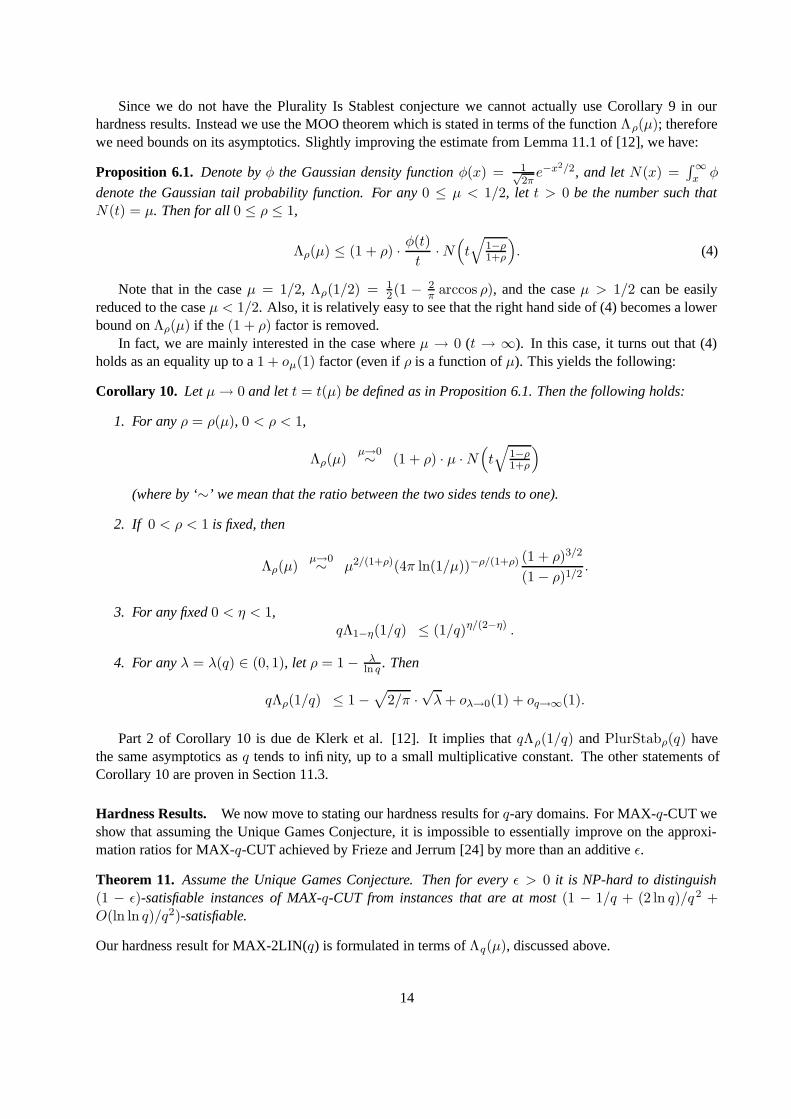
Since we do not have the Plurality Is Stablest conjecture we cannot actually use Corollary 9 in ourhardness results. Instead we use the MOO theorem which is stated in terms of the function Λρ(µ); thereforewe need bounds on its asymptotics. Slightly improving the estimate from Lemma 11.1 of [12], we have:

Proposition 6.1. Denote by φ the Gaussian density function φ(x) = 1√2π

e−x2/2, and let N(x) =∫ ∞x φ

denote the Gaussian tail probability function. For any 0 ≤ µ < 1/2, let t > 0 be the number such thatN(t) = µ. Then for all 0 ≤ ρ ≤ 1,

Λρ(µ) ≤ (1 + ρ) · φ(t)

t· N

(t√

1−ρ1+ρ

). (4)

Note that in the case µ = 1/2, Λρ(1/2) = 12(1 − 2

π arccos ρ), and the case µ > 1/2 can be easilyreduced to the case µ < 1/2. Also, it is relatively easy to see that the right hand side of (4) becomes a lowerbound on Λρ(µ) if the (1 + ρ) factor is removed.

In fact, we are mainly interested in the case where µ → 0 (t → ∞). In this case, it turns out that (4)holds as an equality up to a 1 + oµ(1) factor (even if ρ is a function of µ). This yields the following:

Corollary 10. Let µ → 0 and let t = t(µ) be defined as in Proposition 6.1. Then the following holds:

1. For any ρ = ρ(µ), 0 < ρ < 1,

Λρ(µ)µ→0∼ (1 + ρ) · µ · N

(t√

1−ρ1+ρ

)

(where by ‘∼’ we mean that the ratio between the two sides tends to one).

2. If 0 < ρ < 1 is fixed, then

Λρ(µ)µ→0∼ µ2/(1+ρ)(4π ln(1/µ))−ρ/(1+ρ) (1 + ρ)3/2

(1 − ρ)1/2.

3. For any fixed 0 < η < 1,qΛ1−η(1/q) ≤ (1/q)η/(2−η) .

4. For any λ = λ(q) ∈ (0, 1), let ρ = 1 − λln q . Then

qΛρ(1/q) ≤ 1 −√

2/π ·√

λ + oλ→0(1) + oq→∞(1).

Part 2 of Corollary 10 is due de Klerk et al. [12]. It implies that qΛρ(1/q) and PlurStabρ(q) havethe same asymptotics as q tends to infinity, up to a small multiplicative constant. The other statements ofCorollary 10 are proven in Section 11.3.

Hardness Results. We now move to stating our hardness results for q-ary domains. For MAX-q-CUT weshow that assuming the Unique Games Conjecture, it is impossible to essentially improve on the approxi-mation ratios for MAX-q-CUT achieved by Frieze and Jerrum [24] by more than an additive ε.

Theorem 11. Assume the Unique Games Conjecture. Then for every ε > 0 it is NP-hard to distinguish(1 − ε)-satisfiable instances of MAX-q-CUT from instances that are at most (1 − 1/q + (2 ln q)/q2 +O(ln ln q)/q2)-satisfiable.

Our hardness result for MAX-2LIN(q) is formulated in terms of Λq(µ), discussed above.

14

Theorem 12. Assume the Unique Games Conjecture. Then for every q ≥ 2, ρ ∈ [0, 1] and ε > 0, given aninstance of MAX-2LIN(q), it is NP-hard to distinguish between the case where it is at least (ρ+ 1

q (1−ρ)−ε)-

satisfiable and the case where it is at most (qΛρ(1q ) + ε)-satisfiable. Furthermore, this holds even for

instances in which all equations are of the form xi − xj = c.

Using the asymptotics of Λρ(µ) given above in Corollary 10, we have:

Corollary 13. Assume the Unique Games Conjecture. Then for every fixed η > 0 there exists q0 = q0(η)such that for every fixed q > q0 the following holds. Given an instance of MAX-2LIN(q), it is NP-hard todistinguish between the case where the instance is at least (1 − η)-satisfiable and the case where it is atmost (1/q)η/(2−η) -satisfiable.

Corollary 14. Assume the Unique Games Conjecture, and let λ = λ(q) ∈ (0, 1). Given an instance of MAX-2LIN(q), it is NP-hard to distinguish between the case where the instance is at least (1 − λ

ln q )-satisfiableand the case where it is at most s-satisfiable, where

s = 1 −√

2/π ·√

λ + oλ→0(1) + oq→∞(1).

Note that MAX-2LIN(q) is itself essentially an instance of Unique Label Cover, except for the fact thatthe variable/equation structure need not be bipartite. But in fact, it is easy to observe that the “non-bipartite”version of the Unique Games Conjecture is equivalent to the usual Unique Games Conjecture [38] (up toa factor of 2 in the soundness). Hence Theorem 12 and its corollaries may be viewed as concerning theallowable parameter tradeoffs in the Unique Games Conjecture. In particular, Corollary 13 implies:

Corollary 15. The Unique Games Conjecture holds if and only if it holds as follows: For every η > 0 andlabel set size q (sufficiently large as a function of η), it is NP-hard to distinguish whether the Unique LabelCover problem with label set size q has optimum at least 1 − η or at most (1/q)η/(2−η) .

(The factor of 2 lost in soundness from passing to a bipartite version can be absorbed since the soundnessobtained in the proof of Corollary 13 is actually stronger by a factor of (log q)Ω(1).)

Recently, a result of Charikar, Makarychev, and Makarychev [10] showed that the parameters in Corol-lary 15 are almost optimal. They give an algorithm for Unique Label Cover with label set size q that, givenan instance with optimum (1− η), outputs an assignment which satisfies at least a (1/q)η/(2−3η) -fraction ofthe constraints.

7 Definitions and technical preliminaries

In this section we give some definitions and make some technical observations concerning the Majority IsStablest theorem, reducing it to a form which is useful for our MAX-CUT reduction.

7.1 MAX-CUT and MAX-2SAT

For the majority of this paper we will be concerned with the MAX-CUT problem; we will also later considerthe MAX-2SAT problem. We give the formal definitions of these problems below.

Definition 9 (MAX-CUT). Given an undirected graph G = (V,E), the MAX-CUT problem is that offinding a partition C = (V1, V2) which maximizes the size of the set (V1 ×V2)∩E. Given a weight-functionw : E → R+, the weighted MAX-CUT problem is that of maximizing

∑

e∈(V1×V2)∩E

w(e).

15

Definition 10 (MAX-2SAT). An instance of the MAX-2SAT problem is a set of boolean variables and a setof disjunctions over two literals each, where a literal is either a variable or its negation. The problem isto assign the variables so that the number of satisfied literals is maximized. Given a nonnegative weightfunction over the set of disjunctions, the weighted MAX-2SAT problem is that of maximizing the sum ofweights of satisfied disjunctions.

As we noted earlier, [11] implies that the achievable approximation ratios for the weighted versions ofthe above two problems are the same, up to an additive o(1), as the approximation ratios of the respectivenon-weighted versions. Hence in this paper we do not make a distinction between the weighted and thenon-weighted versions.

7.2 Analytic notions

In this paper we treat the bit TRUE as −1 and the bit FALSE as 1; we consider functions f : −1, 1n → R

and say a function is boolean-valued if its range is −1, 1. The domain −1, 1n is viewed as a probabilityspace under the uniform measure and the set of all functions f : −1, 1n → R as an inner product spaceunder 〈f, g〉 = E[fg]. The associated norm in this space is given by ‖f‖2 =

√E[f2].

Fourier expansion. For S ⊆ [n], let χS denote the parity function on S, χS(x) =∏

i∈S xi. It is wellknown that the set of all such functions forms an orthonormal basis for our inner product space and thusevery function f : −1, 1n → R can be expressed as

f =∑

S⊆[n]

f(S)χS .

Here the real quantities f(S) = 〈f, χS〉 are called the Fourier coefficients of f and the above is calledthe Fourier expansion of f . Plancherel’s identity states that 〈f, g〉 =

∑S f(S)g(S) and in particular,

‖f‖22 =

∑S f(S)2. Thus if f is boolean-valued then

∑S f(S)2 = 1, and if f : −1, 1n → [−1, 1] then∑

S f(S)2 ≤ 1. We speak of f ’s squared Fourier coefficients as weights, and we speak of the sets S beingstratified into levels according to |S|. So for example, by the weight of f at level 1 we mean

∑|S|=1 f(S)2.

The Bonami-Beckner operator. For any ρ ∈ [−1, 1] we define the Bonami-Beckner operator Tρ, a linearoperator on the space of functions −1, 1n → R, by Tρ(f)(x) = E[f(y)]; where each coordinate yi ofy is independently chosen to be xi with probability 1

2 + 12ρ and −xi with probability 1

2 − 12ρ. It is easy

to check that Tρ(f) =∑

S ρ|S|f(S)χS . It is also easy to verify the following relation between Tρ and thenoise stability (see Definition 3).

Proposition 7.1. Let f : −1, 1n → R and ρ ∈ [−1, 1]. Then

Sρ(f) = 〈f, Tρf〉 =∑

S⊆[n]

ρ|S|f(S)2.

The following identity is a well-known one, giving a Fourier analytic formula for the influences of a coordi-nate on a function (see Definition 2).

Proposition 7.2. Let f : −1, 1n → R. Then for every i ∈ [n],

Infi(f) =∑

S3i

f(S)2. (5)

16

Once we have the Fourier analytic formula for the influence, we can consider the contribution to theinfluence of characters of bounded size.

Definition 11. Let f : −1, 1n → R, and let i ∈ [n]. The k-degree influence of coordinate i on f is definedby

Inf≤ki (f) =

∑

S3i|S|≤k

f(S)2.

7.3 Different forms of the Majority Is Stablest theorem

Recall the Majority Is Stablest theorem:

Majority Is Stablest theorem: Fix ρ ∈ [0, 1). Then for any ε > 0 there is a small enough δ = δ(ε, ρ) > 0such that if f : −1, 1n → [−1, 1] is any function satisfying

E[f ] = 0, and

Infi(f) ≤ δ for all i = 1 . . . n,

thenSρ(f) ≤ 1 − 2

π arccos ρ + ε.

In the MAX-CUT reduction we need a slightly altered version of the Majority Is Stablest theorem. First,we can replace influences by low-degree influences:

Proposition 7.3. The Majority Is Stablest theorem remains true if the assumption that Inf i(f) ≤ δ for all i

is replaced by the assumption that Inf≤k′

i (f) ≤ δ′, where δ′ and k′ are universal functions of ε and ρ.

Proof. Fix ρ < 1 and ε > 0. Choose γ such that ρk(1−(1−γ)2k) < ε/4 for all k. Let δ be chosen such thatif Infi(g) ≤ δ for all i then Sρ(g) ≤ 1− 2

π arccos ρ+ε/4. Choose δ′ = δ/2 and k′ such that (1−γ)2k′< δ′.

Let f be a function satisfying Inf≤k′

i (f) ≤ δ′ and let g = T1−γf . Note that

Infi(g) ≤∑

S:i∈S,|S|≤k′

f(S)2 + (1 − γ)2k′∑

S:i∈S,|S|≤k′

f(S)2 < δ′ + δ′ = δ

for all i.It now follows that Sρ(g) ≤ 1 − 2

π arccos ρ + ε/4 and therefore

Sρ(f) = Sρ(g) +∑

S

(ρ|S|(1 − (1 − γ)|S|))f(S)2 < 1 − 2π arccos ρ + 3ε/4.

Second, we need to treat the case of negative ρ:

Proposition 7.4. The Majority Is Stablest theorem is true ‘in reverse’ for ρ ∈ (−1, 0]. That is, Sρ(f) ≥1 − 2

π arccos ρ − ε, and furthermore, the assumption E[f ] = 0 becomes unnecessary.

Proof. Let f : −1, 1n → [−1, 1] satisfy Inf i(f) ≤ δ for all i. Let g be the odd part of f , g(x) = (f(x)−f(−x))/2 =

∑|S| odd f(S)xS . Then E[g] = 0, Inf i(g) ≤ Infi(f) for all i, and Sρ(f) ≥ Sρ(g) = −S−ρ(g),

which exceeds −(1 − 2π arccos ρ + ε) by the Majority Is Stablest theorem applied to g.

17

Combining the above two propositions we get the result that will be used in our reduction from UniqueLabel Cover to 2-bit CSPs:

Proposition 7.5. Fix ρ ∈ (−1, 0]. Then for any ε > 0 there is a small enough δ = δ(ε, ρ) > 0 and a largeenough k = k(ε, ρ) such that if f : −1, 1n → [−1, 1] is any function satisfying

Inf≤ki (f) ≤ δ for all i = 1 . . . n,

thenSρ(f) ≥ 1 − 2

π arccos ρ − ε.

8 Reduction from Unique Label Cover to MAX-CUT

In this section we prove Theorem 1.

8.1 The PCP

We construct a PCP that reads two bits from the proof and accepts if and only if the two bits are unequal.The completeness and soundness are c and s respectively. This implies that MAX-CUT is NP-hard to ap-proximate within any factor greater than s/c. The reduction from the PCP to MAX-CUT is straightforwardand can be considered standard: Let the bits in the proof be vertices of a graph and the tests of the verifier bethe edges of the graph. The −1, 1 assignment to bits in the proof corresponds to a partition of the graphinto two parts and the tests for which the verifier accepts correspond to the edges cut by this partition.

The completeness and soundness properties of the PCP rely on the Unique Games Conjecture and theMajority Is Stablest theorem. The Unique Label Cover instance given by the Unique Games Conjectureserves as the PCP outer verifier. The soundness of the Long Code-based inner verifier is implied by theMajority Is Stablest theorem.

Before we explain the PCP test, we need some notation. For x ∈ −1, 1M and a bijection σ : [M ] →[M ], let x σ denote the string (xσ(1), xσ(2), . . . , xσ(M)). For x, µ ∈ −1, 1M , let xµ denote the M -bitstring that is the coordinatewise product of x and µ.

The PCP verifier is given the Unique Label Cover instance L(V,W,E, [M ], σv,w(v,w)∈E) given bythe Unique Games Conjecture. Using a result from [37] we may assume the bipartite graph is regular on theV side, so that choosing a uniformly random vertex v ∈ V and a random neighbor w of v yields a uniformlyrandom edge (u,w). We assume that the Unique Label Cover instance is either (1−η)-satisfiable or at mostγ-satisfiable, where we will choose the values of η and γ to be sufficiently small later. The verifier expectsas a proof the Long Code of the label of every vertex w ∈ W . The verifier is parameterized by ρ ∈ (−1, 0).

The PCP verifier for MAX-CUT with parameter −1 < ρ < 0

• Pick a vertex v ∈ V at random and two of its neighbors w,w ′ ∈ W at random. Let σ = σv,w andσ′ = σv,w′ be the respective bijections for edges (v, w) and (v, w ′).

• Let fw and fw′ be the supposed Long Codes of the labels of w and w′ respectively.

• Pick x ∈ −1, 1M at random.

• Pick µ ∈ −1, 1M by choosing each coordinate independently to be 1 with probability 12 + 1

2ρ < 12

and −1 with probability 12 − 1

2ρ > 12 .

• Accept ifffw(x σ) 6= fw′((x σ′)µ).

18

8.2 Completeness

It is easy to see that the completeness of the verifier is at least (1 − 2η)(12 − 12ρ). Assume that the Label

Cover instance has a labeling that satisfies a 1−η fraction of edges. Take this labeling and encode the labelsvia Long Codes. We will show that the verifier accepts with probability at least (1 − 2η)(12 − 1

2ρ).With probability at least 1 − 2η, both the edges (v, w) and (v, w ′) are satisfied by the labeling. Let the

labels of v, w,w′ be i, j, j′ ∈ [M ] respectively such that σ(j) = i = σ ′(j′). The functions fw, fw′ are theLong Codes of j, j ′ respectively. Hence

fw(x σ) = xσ(j) = xi, fw′((x σ′)µ) = xσ′(j′)µj′ = xiµj′

Thus the two bits are unequal (and the test accepts) iff µj′ = −1 which happens with probability 12 − 1

2ρ.

8.3 Soundness

We prove soundness in the contrapositive direction, as is usual in PCP proofs: Assume that some supposedLong Codes fw cause the PCP verifier to accept with probability at least (arccos ρ)/π + ε. We use Fouriermethods to “list-decode” the Long Codes and extract a labeling for the Unique Label Cover instance thatsatisfies some γ′ = γ′(ε, ρ) fraction of its edges. Since this constant does not depend on the Label Coverlabel set size M , we can take M large enough in the Unique Games Conjecture to get soundness γ < γ ′, asrequired.

We first analyze the probability of acceptance for the PCP verifier by arithmetizing it as follows:

Pr[acc] = Ev,w,w′,x,µ

[1

2− 1

2fw(x σ)fw′((xµ) σ′)

]

=1

2− 1

2· E

v,x,µ

[E

w,w′[fw(x σ)fw′((xµ) σ′)]

]

=1

2− 1

2· E

v,x,µ

[Ew

[fw(x σ)] · Ew′

[fw′((xµ) σ′)]]

(using independence of w and w′)

=1

2− 1

2· E

v,x,µ[gv(x)gv(xµ)] (where we define gv(z) = E

w∼v[fw(z σv,w)])

=1

2− 1

2·E

v[Sρ(gv)].

Now if Pr[acc] ≥ (arccos ρ)/π + ε, then for at least an ε/2 fraction of v ∈ V ,

Sρ(gv) ≤ 1 − 2π arccos ρ − ε.

We say that such a vertex v is “good”. For every good v, we apply the Majority Is Stablest theorem inthe guise of Proposition 7.5 to conclude that gv has at least one coordinate, say j, with k-degree influenceat least δ. We shall give the label j to v. In this way, all good v ∈ V are labeled. For a good v, sinceInf≤k

j (gv) ≥ δ, we have

δ ≤∑

S3j|S|≤k

gv(S)2 =∑

S3j|S|≤k

Ew

[fw(σ−1(S))]2 ≤∑

S3j|S|≤k

Ew

[fw(σ−1(S))2] = Ew

[Inf≤k

σ−1(j)(fw)

]. (6)

For every w ∈ W , define the set of candidate labels for w to be

Cand[w] = i ∈ [M ] : Inf≤ki (fw) ≥ δ/2.

19

Since∑

i Inf≤ki (fw) ≤ k, we conclude that |Cand[w]| ≤ 2k/δ. Inequality (6) implies that for every good v,

at least a δ/2 fraction of neighbors w of v have Inf≤k

σ−1v,w(j)

(f) ≥ δ/2, and therefore σ−1(j) ∈ Cand[w]. Now

we label each vertex w ∈ W by choosing a random element of Cand[w] (or any label if this set is empty). Itfollows that among the set of edges adjacent to good vertices v, at least a (δ/2)(δ/2k)-fraction are satisfiedin expectation. Thus it follows that there is labeling for all vertices which satisfies a γ′ = (ε/2)(δ/2)(δ/2k)fraction of all edges. This completes the proof of soundness.

8.4 Completion of the proof of Theorem 1

We have just shown how to reduce Unique Label Cover instances to MAX-CUT instances with completeness(12 − 1

2ρ)(1 − 2η) and soundness (arccos ρ)/π + ε, where η and ε can be made arbitrarily small. The mainstatement of Theorem 1 follows by slightly modifying ρ to move the completeness correction (1 − 2η) intothe soundness correction ε. This result implies a hardness of approximation factor of

arccos(ρ)/π12 − 1

2ρ+ ε

for any constant −1 < ρ < 0 and ε > 0; choosing ρ = ρ∗ as stated in the theorem yields the desiredhardness factor αGW + ε.

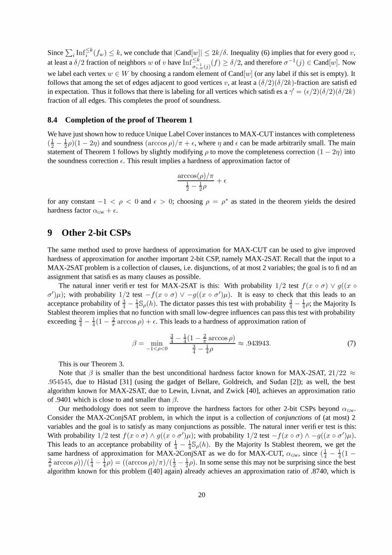
9 Other 2-bit CSPs

The same method used to prove hardness of approximation for MAX-CUT can be used to give improvedhardness of approximation for another important 2-bit CSP, namely MAX-2SAT. Recall that the input to aMAX-2SAT problem is a collection of clauses, i.e. disjunctions, of at most 2 variables; the goal is to find anassignment that satisfies as many clauses as possible.

The natural inner verifier test for MAX-2SAT is this: With probability 1/2 test f(x σ) ∨ g((x σ′)µ); with probability 1/2 test −f(x σ) ∨ −g((x σ ′)µ). It is easy to check that this leads to anacceptance probability of 3

4 − 14Sρ(h). The dictator passes this test with probability 3

4 − 14ρ; the Majority Is

Stablest theorem implies that no function with small low-degree influences can pass this test with probabilityexceeding 3

4 − 14(1 − 2

π arccos ρ) + ε. This leads to a hardness of approximation ration of

β = min−1<ρ<0

34 − 1

4(1 − 2π arccos ρ)

34 − 1

4ρ≈ .943943. (7)

This is our Theorem 3.Note that β is smaller than the best unconditional hardness factor known for MAX-2SAT, 21/22 ≈

.954545, due to Hastad [31] (using the gadget of Bellare, Goldreich, and Sudan [2]); as well, the bestalgorithm known for MAX-2SAT, due to Lewin, Livnat, and Zwick [40], achieves an approximation ratioof .9401 which is close to and smaller than β.

Our methodology does not seem to improve the hardness factors for other 2-bit CSPs beyond αGW.Consider the MAX-2ConjSAT problem, in which the input is a collection of conjunctions of (at most) 2variables and the goal is to satisfy as many conjunctions as possible. The natural inner verifier test is this:With probability 1/2 test f(x σ) ∧ g((x σ ′)µ); with probability 1/2 test −f(x σ) ∧ −g((x σ ′)µ).This leads to an acceptance probability of 1

4 − 14Sρ(h). By the Majority Is Stablest theorem, we get the

same hardness of approximation for MAX-2ConjSAT as we do for MAX-CUT, αGW, since ( 14 − 1

4 (1 −2π arccos ρ))/( 1

4 − 14ρ) = ((arccos ρ)/π)/( 1

2 − 12ρ). In some sense this may not be surprising since the best

algorithm known for this problem ([40] again) already achieves an approximation ratio of .8740, which is

20

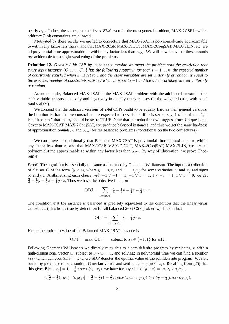
nearly αGW. In fact, the same paper achieves .8740 even for the most general problem, MAX-2CSP in whicharbitrary 2-bit constraints are allowed.

Motivated by these results we are led to conjecture that MAX-2SAT is polynomial-time approximableto within any factor less than β and that MAX-2CSP, MAX-DICUT, MAX-2ConjSAT, MAX-2LIN, etc. areall polynomial-time approximable to within any factor less than αGW. We will now show that these boundsare achievable for a slight weakening of the problems.

Definition 12. Given a 2-bit CSP, by its balanced version we mean the problem with the restriction thatevery input instance C1, . . . , Cm has the following property: for each i = 1 . . . n, the expected numberof constraints satisfied when xi is set to 1 and the other variables are set uniformly at random is equal tothe expected number of constraints satisfied when xi is set to −1 and the other variables are set uniformlyat random.

As an example, Balanced-MAX-2SAT is the MAX-2SAT problem with the additional constraint thateach variable appears positively and negatively in equally many clauses (in the weighted case, with equaltotal weight).

We contend that the balanced versions of 2-bit CSPs ought to be equally hard as their general versions;the intuition is that if more constraints are expected to be satisfied if xi is set to, say, 1 rather than −1, itis a “free hint” that the xi should be set to TRUE. Note that the reductions we suggest from Unique LabelCover to MAX-2SAT, MAX-2ConjSAT, etc. produce balanced instances, and thus we get the same hardnessof approximation bounds, β and αGW, for the balanced problems (conditional on the two conjectures).

We can prove unconditionally that Balanced-MAX-2SAT is polynomial-time approximable to withinany factor less than β, and that MAX-2CSP, MAX-DICUT, MAX-2ConjSAT, MAX-2LIN, etc. are allpolynomial-time approximable to within any factor less than αGW. By way of illustration, we prove Theo-rem 4:

Proof. The algorithm is essentially the same as that used by Goemans-Williamson. The input is a collectionof clauses C of the form (y ∨ z), where y = σixi and z = σjxj for some variables xi and xj and signsσi and σj . Arithmetizing each clause with −1 ∨ −1 = 1, −1 ∨ 1 = 1, 1 ∨ −1 = 1, 1 ∨ 1 = 0, we get34 − 1

4y − 14z − 1

4y · z. Thus we have the objective function

OBJ =∑

C=(y∨z)

34 − 1

4y − 14z − 1

4y · z.

The condition that the instance is balanced is precisely equivalent to the condition that the linear termscancel out. (This holds true by definition for all balanced 2-bit CSP problems.) Thus in fact

OBJ =∑

C=(y∨z)

34 − 1

4y · z.

Hence the optimum value of the Balanced-MAX-2SAT instance is

OPT = max OBJ subject to xi ∈ −1, 1 for all i.

Following Goemans-Williamson we directly relax this to a semidefinite program by replacing xi with ahigh-dimensional vector vi, subject to vi · vi = 1, and solving; in polynomial time we can find a solutionvi which achieves SDP − ε, where SDP denotes the optimal value of the semidefinite program. We nowround by picking r to be a random Gaussian vector and setting xi = sgn(r · vi). Recalling from [25] thatthis gives E[xi · xj] = 1 − 2

π arccos(vi · vj), we have for any clause (y ∨ z) = (σixi ∨ σjxj),

E[34 − 14(σixi) · (σjxj)] = 3

4 − 14(1 − 2

π arccos(σivi · σjvj)) ≥ β(34 − 1

4(σivi · σjvj)),

21

where we have used the definition of β and the fact that it is unchanged if we let ρ range over [−1, 1]. Itfollows that E[OBJ] ≥ βSDP ≥ βOPT and the proof is complete.

10 Special cases of the Majority Is Stablest theorem

In this section we describe special cases of the Majority Is Stablest theorem which are of particular interest,and have elementary proofs.

10.1 Weighted majorities

In this subsection we prove Theorem 5, which makes the point that the majority function is not unique as anoise stability maximizer, in the sense that all weighted majority functions with small influences have thesame noise stability, i.e., 1− 2

π arccos ρ. The proof requires a multidimensional version of the Central LimitTheorem with error bounds. We have the following version from [5, Corollary 16.3]:

Theorem 16. Let X1, . . . ,Xn be independent random variables taking values in Rk satisfying:

• E[Xj ] = 0, j = 1 . . . n;

• n−1∑n

j=1 Cov(Xj) = V , where Cov denotes the variance-covariance matrix;

• λ is the smallest eigenvalue of V , Λ is the largest eigenvalue of V ;

• ρ3 = n−1∑n

j=1 E[|Xj |3] < ∞.

Let Qn denote the distribution of n−1/2(X1 + · · · + Xn), let Φ0,V denote the distribution of the k-dimensional Gaussian with mean 0 and variance-covariance matrix V , and let η = Cλ−3/2ρ3n

−1/2, whereC is a certain universal constant.

Then for any Borel set A,|Qn(A) − Φ0,V (A)| ≤ η + B(A),

where B(A) is the following measure of the boundary of A: B(A) = 2 supy∈Rk Φ0,V ((∂A)η′+ y), where

η′ = Λ1/2η and (∂A)η′denotes the set of points within distance η ′ of the topological boundary of A.

Theorem 5 follows from the following two propositions.

Proposition 10.1. Let f : −1, 1n → −1, 1 be any balanced threshold function, f(x) = sgn(a1x1 +· · · anxn)2, where

∑a2

i = 1. Let δ = max|ai|. Then for all ρ ∈ [−1, 1],

Sρ(f) = 1 − 2π arccos ρ ± O(δ(1 − |ρ|)−3/2).

Proposition 10.2. Let f : −1, 1n → −1, 1 be any balanced threshold function, f(x) = sgn(a1x1 +· · · anxn), where

∑a2

i = 1. Let δ = max|ai|. Then maxi Inf i(f) ≥ Ω(δ).

We prove the two propositions below.

2Without loss of generality we assume the linear form is never 0.

22

Proof of Proposition 10.1. Since f is antisymmetric, we only need to prove the result for ρ ∈ [0, 1]. Let xand y be ρ-correlated uniformly random strings, let Xj = ajxj , Yj = ajyj , and Xj = (Xj , Yj) ∈ R2. LetQn denote the distribution of X1 + · · ·+Xn = n−1/2(

√nX1 + · · ·+√

nXn). Since Sρ(f) = 2Pr[f(x) =f(y)]− 1, we are interested in computing 2Qn(A++ ∪A−−)− 1, where A++ denotes the positive quadrantof R2 and A−− denotes the opposite quadrant.

We shall apply Theorem 16. We have E[Xj] = 0 for all j. We have Cov(√

nXj) = na2i

[1 ρρ 1

], and

thus V = n−1∑

Cov(√

nXj) =

[1 ρρ 1

]. The eigenvalues of V are λ = 1 − ρ and Λ = 1 + ρ. Since

|√nXj| is√

2n |ai| with probability 1, ρ3 = n−1∑

E[|√nXj |3] = 23/2n1/2∑ |ai|3 ≤ 23/2n1/2δ. Thus

η = O(1)δ(1 − ρ)−3/2 and η′ = (1 + ρ)1/2η = O(η).It is well known (see, e.g., [1, 26.3.19]) that Φ0,V (A++) = Φ0,V (A−−) = 1/2 − (1/2π) arccos(ρ),

and it is easy to check that B(A++ ∪ A−−) = O(η′). Thus by Theorem 16 we get Qn(A++ ∪ A−−) =1 − (arccos ρ)/π ± O(η) and the theorem follows.

Proof of Proposition 10.2. We may assume without loss of generality that δ = a1 ≥ a2 ≥ · · · ≥ an ≥ 0.Letting Xi denote the random variable aixi, we will prove that Inf1(f) ≥ Ω(δ) by proving that

Pr[|X2 + · · · + Xn| ≤ δ] ≥ Ω(δ). (8)

Let C be the constant hidden in the O(·) in the final part of the Berry-Esseen theorem, Theorem 18. Inproving (8) we may also assume without loss of generality that

1 − 100C2δ2 ≥ 1/4; (9)

i.e., δ is not too large. We may also assume C is an integer.Let m = 100C2 + 2. We will split into two cases, depending on the magnitude of am. In either case,

we shall apply the Berry-Esseen theorem to the sequence Xm, . . . , Xn. We have

σ = (

n∑

j=m

E[Xj ]2)1/2 = (

n∑

j=m

a2j )

1/2 ≥ (1 − (m − 2)δ2)1/2 ≥ (1 − 100C2δ2)1/2 ≥ 1/2,

where we have used (9). We also have ρ3 =∑n

j=m E[|Xj |3] ≤∑n

j=m amE[X2j ] = amσ2, so the error term

in the conclusion of the theorem, O(ρ3/σ3), is at most Cam/σ ≤ 2Cam.

Case 1: am ≤ 110C δ. In this case, by the Berry-Esseen theorem we have that

Pr[Xm + · · · + Xn ∈ [0, δ]] ≥ Φ([0, δ]) − 2Cam ≥ δφ(δ) − δ/5 ≥ .04δ,

where we have used the fact that φ(δ) ≥ .24 for δ ≤ 1. On the other hand, since a2, . . . , am−1 are all atmost δ, it is easy to fix particular signs yi ∈ −1, 1 such that

∑m−1i=2 aiyi ∈ [−δ, 0]. These signs occur with

probability 2−m+2, which is at least 2−100C2

. Thus with probability at least .04 · 2−100C2

δ = Ω(δ) bothevents occur, and |X2 + · · · + Xn| ≤ δ as desired.

Case 2: am ≥ 110C δ. In this case, we apply the Berry-Esseen theorem to the interval [−10Cδ, 10Cδ] and

merely use the fact that am ≤ δ. We conclude that

Pr[Xm + · · · + Xn ∈ [−10Cδ, 10Cδ]] ≥ Φ([−10Cδ, 10Cδ]) − 2Cδ

≥ 20Cδ · φ(10Cδ) − 2Cδ ≥ 20Cδ · 1√2π

(1 − (10Cδ)2/2) − 2Cδ ≥ 4Cδ,

23

where we have used (9) in the last step to infer 1 − (10Cδ)2/2 ≥ 5/8. Given Xm + · · · + Xn = t ∈[−10Cδ, 10Cδ], it is easy to choose particular signs y2, . . . , ym−1 such that t +

∑m−1i=2 aiyi ∈ [−δ, δ]. This

uses the fact that each ai is at least 110C δ and hence

∑m−1i=2 ai ≥ 100C2 1

10C δ ≥ 10Cδ; it also uses the fact

that each ai is at most δ. Once again, these signs occur for x2, . . . , xm−1 with probability at least 2−100C2

.Thus |X2 + · · · + Xn| ≤ δ happens with probability at least 4C2−100C2

δ = Ω(δ), as desired.

10.2 Bounds for the weight on the first level

Applying the Majority Is Stablest theorem for extremely small ρ, it follows that functions with small influ-ences have no more weight at level 1 than Majority has, viz., 2

π (up to o(1)). This fact, stated in Theorem 6,has a very elementary proof which also provides a better bound on the additive term corresponding to themaximal influence:

Proof of Theorem 6. Let ` denote the linear part of f , `(x) =∑n

i=1 f(i)xi. We have that |f(i)| ≤Infi(f) ≤ δ for all i. Now

∑|S|=1 f(S)2 = ‖`‖2

2 and

‖`‖22 = 〈f, `〉

≤ ‖f‖∞‖`‖1

≤ ‖`‖1.

Since all of `’s coefficients are small, smaller than δ, we expect ` to behave like a Gaussian with meanzero and standard deviation ‖`‖2; such a Gaussian has L1-norm equal to

√2/π‖`‖2. Several error bounds

on the Central Limit Theorem exist to this effect; the sharpest is a result of Konig, Schutt, and Tomczak-Jaegermann [39] which implies that ‖`‖1 ≤

√2/π‖`‖2 + (C/2)δ. Thus

‖`‖22 ≤

√2/π‖`‖2 + (C/2)δ,

hence ‖`‖2 ≤√

1/2π +√

1/2π + Cδ/2 and therefore ‖`‖22 ≤ 2/π + Cδ.

In the following we improve the bound on the weight of the first level for not necessarily balancedfunctions with low influences. This result should be compared to the following theorem of Talagrand [49]:

Theorem 17. (Talagrand) Suppose f : −1, 1n → −1, 1 satisfies Pr[f = 1] = p ≤ 1/2. Then

∑

|S|=1

f(S)2 ≤ O(p2 log(1/p)).

We will need the following Berry-Esseen theorem, which gives error bounds for the Central Limit The-orem [19]:

Theorem 18. (Berry-Esseen) Let X1, . . . , Xn be a sequence of independent random variables satisfyingE[Xj ] = 0 for all j, (

∑nj=1 E[X2

j ])1/2 = σ, and∑n

j=1 E[|Xj |3] = ρ3. Let Q = σ−1(X1 + · · · + Xn), letF denote the cumulative distribution function of Q, F (x) = Pr[Q ≤ x], and let Φ denote the cumulativedistribution function of a standard normal random variable. Then

supx

(1 + |x|3)|F (x) − Φ(x)| ≤ O(ρ3/σ3).

In particular, if A is any interval in R, |Pr[Q ∈ A] − Pr[N(0, 1) ∈ A]| ≤ O(ρ3/σ3).

We now prove Theorem 7.

24

Proof of Theorem 7. It will be more convenient to work with the [0, 1] valued-function g = 12 + 1

2f and

prove that∑

|S|=1 g(S)2 ≤(U(µ) + max1,

√|Φ−1(µ)|O(

√δ)

)2. Note that µ = E[g]. We will assume

without loss of generality that µ ≥ 1/2 (otherwise look at 12 − 1

2f ).Let τ denote (

∑|S|=1 g(S)2)1/2. As in the proof of Theorem 6, we let ` be the linear part of g and

we know that all of `’s coefficients are at most δ/2. The function L = `/τ =∑

S g(S)χS/τ is a sum ofindependent random variables XS = g(S)χS/τ . Clearly E[XS ] = 0 for all S. Moreover,

∑S E[X2

S ] = 1and

∑S E[X3

S ] ≤ maxS |XS | ≤ δ/(2τ).Now τ2 = 〈g, `〉 and therefore τ = 〈g, L〉. We will show below that

τ = 〈g, L〉 ≤ U(µ) + max1, |Φ−1(µ)|O(δ/τ). (10)

Multiplying by τ implies that

(τ − U(µ)

2

)2

≤ U2(µ)/4 + max1, |Φ−1(µ)|O(δ).

which in turn implies thatτ ≤ U(µ) + max1,

√|Φ−1(µ)|O(

√δ)

Finally, we will conclude that

τ2 ≤(U(µ) + max1,

√|Φ−1(µ)|O(

√δ)

)2.

We now prove (10). Let t be a number such that Pr[L > t] = µ. Since g is a [0, 1] valued-function itfollows that 〈g, L〉 ≤ E[1L>tL].

Letting F denote the cumulative distribution function of L, the Berry-Esseen theorem implies thatsupx(1 + |x|3)|F (x) − Φ(x)| ≤ O(δ/τ). In particular, |Pr[L > t] − Pr[N(0, 1) > t]| ≤ O(δ/(τ(1 + t3))and hence

|µ − Φ(−t)| ≤ O

(δ

τ(1 + t3)

)(11)

Note that the function U satisfies

U ′(x) = φ′(Φ−1(x)) · ((Φ−1(x))′) = −Φ−1(x)φ(Φ−1(x))1

φ(Φ−1(x))= −Φ−1(x).

Therefore U ′′(x) = −1/φ(Φ−1(x)) = −1/U(x). It follows that U is concave.We now estimate U(µ) − φ(t). Since U ′ is a monotone function, it follows that

|U(µ) − φ(t)| = |U(Φ(−t)) − U(µ)| ≤ |Φ(−t) − µ|max|U ′(Φ(−t))|, |U ′(µ)| (12)

≤ max|t|,Φ−1(µ)O(δ/(τ(1 + t3))) ≤ max1, |Φ−1(µ)|O(δ/τ).

25

Further,

〈g, L〉 ≤ E[1L>tL] = tPr[L > t] +

∫ ∞

tPr[L > x] dx

= tPr[L > t] +

∫ ∞

tPr[N(0, 1) > x] dx +

∫ ∞

t(F (x) − Φ(x)) dx

= tµ − tΦ(−t) + φ(t) +

∫ ∞

t(F (x) − Φ(x)) dx

≤ φ(t) + |t| · |µ − Φ(−t)| +∫ ∞

t|F (x) − Φ(x)| dx

≤ φ(t) +|t|

1 + |t|3 O(δ/τ) + O(δ/τ)

∫ ∞

t1/(1 + |x|3) dx ((11) and Berry-Esseen)

= φ(t) + O

(δ

τ(1 + t2)

)(by (12))

≤ U(µ) + max1, |Φ−1(µ)|O(δ/τ).

which proves (10) as needed.

11 Constraint satisfaction problems over [q]

So far in this paper we have mostly focused on 2-CSPs in which the variables are binary — i.e., take valuesin the alphabet −1, 1. The exception is the Unique Label Cover problem, which can be thought of as a2-CSP where the set of values a variable can take is very large. In this section we develop our techniquesfor 2-CSPs over such large alphabets; specifically, the alphabet [q] = 1, 2, . . . , q for q ≥ 2. We willbe concerned in particular with the MAX-2LIN(q) and MAX-q-CUT (i.e. Approximate Graph q-Coloring)problems, and we will mostly be interested in the asymptotics when q → ∞.

11.1 Γ-MAX-2LIN(q) and MAX-q-CUT

The MAX-q-CUT problem is a natural generalization of MAX-CUT; its formal definition is as follows:

Definition 13 (MAX-q-CUT). Given a weighted graph G = (V,W ) where W : V × V → R+, the MAX-q-CUT problem is that of finding a partition of V into q sets V1, . . . , Vq in such a way as to maximize theweight of edges between the different parts,

∑i6=j

∑v∈Vi,w∈Vj

W (v, w).

The MAX-2LIN(q) problem is defined as follows:

Definition 14 (MAX-2LIN(q)). Given a system of m linear equations mod q each having at most 2 vari-ables, along with nonnegative weights w1, . . . , wm for these equations, the MAX-2LIN(q) problem is to findan assignment to the variables maximizing the total weight of satisfied equations.

Observe that the MAX-2-CUT problem can be viewed as a special case of the MAX-2LIN(2) problem,by associating the vertices with variables and the edges with equations xu − xv = 1. However for larger q,MAX-q-CUT is more naturally viewed as a special case of the problem of finding assignments for 2-variablelinear inequations mod q.

The best approximation algorithm for MAX-q-CUT was obtained by Frieze and Jerrum in [24]; thispaper gives a (1 − 1/q + 2(ln q)/q2)-approximation. The best NP-hardness result known is due to Kann,

26

Khanna, Lagergren, and Panconesi [] who proved that (1 − 1/(34q))-approximating is hard. As for the ap-proximability of MAX-2LIN(q), the best algorithm known was given very recently by Charikar, Makarychev,and Makarychev in [], as discussed in Subsection 6.3 (their algorithm is actually for the more general prob-lem of not-necessarily-bipartite Unique Label Cover with label size q). When the optimal fraction of satis-fiable constraints is 1 − η, their semidefinite programming algorithm produces a solution satisfying abouta fraction (1/q)η/(2−3η) . The best known NP-hardness results come from a recent work of Feige and Re-ichman [20]. They show that it is NP-hard to approximate MAX-2LIN(q) to within a factor of 1/qβ forsome universal constant β > 0; however this hardness is located at a gap of ε vs. ε/qβ . In particular, givenan instance with optimum fraction 1 − η, Feige and Reichman can only show that it is NP-hard to find asolution with value 1−Cη for some relatively small constant C > 1. Thus with current knowledge, given a(1− η)-satisfiable instance, we don’t know whether one can satisfy almost all the constraints in polynomialtime, or whether it is impossible to go beyond a very small fraction of them.

A special case of the MAX-2LIN(q) problem which seems somewhat easier algorithmically ([],[]) occurswhen all the equations in the instance are of the form xi − xj = cij .

Definition 15 (Γ-MAX-2LIN(q)). Γ-MAX-2LIN(q) is the special case of MAX-2LIN(q) in which each equa-tion is of the form xi − xj = cij .

Our hardness results will hold even for Γ-MAX-2LIN(q). The Γ notation is essentially from Hastad [31];we use it because our results actually hold equally well for the problem of satisfying equations of the formxix

−1j = cij over any fixed abelian group Γ of order q, not just Zq.

11.2 Analytic notions

We would like to generalize our notions of noise stability, influences, and Fourier expansions to q-ary func-tions, f : [q]n → [q]. Some of the definitions below were already given in Subsection 4.2, but we repeatthem here for clarity and convenience.

The way we treat the finite set [q] in the domain and in the range of q-ary functions will be different.In the domain, [q] and [q]n will be treated simply as finite probability spaces under the uniform measure,with no extra structure. In the range, we would like to embed [q] into a larger space. Recall that for booleanfunction we identified the range with the two points −1, 1 ∈ R and then considered relaxed functions takingvalues in their convex hull. In the q-ary case we identify the elements of [q] with the standard basis vectorsin Rq. A relaxed q-ary function will thus map [q]n into the simplex which is the convex hull of these vectors.

Definition 16. Let ∆q denote the (q − 1)-dimensional simplex naturally embedded in Rq; i.e., the convexhull of the q standard basis vectors. We call functions f : [q]n → ∆q relaxed q-ary functions.

We will also define the notion of a balanced function:

Definition 17. A function f : [q]n → [q] is called balanced if it obtains each value i ∈ [q] in its rangeequally often. A relaxed function f : [q]n → ∆q is called balanced if E[f(x)] = (1/q, . . . , 1/q).

Since a relaxed q-ary function f maps [q]n into Rq, it can be viewed as a vector f = (f1, . . . , fq) ofreal-valued functions over [q]n. We define the noise stability both for real-valued and ∆q-valued functions.

Definition 18. Let − 1q−1 ≤ ρ ≤ 1 and let x and y be [q]n-valued random variables. We say that x and y are

a ρ-correlated pair if x is uniformly distributed on [q]n, and y is formed from x by choosing each yi so thatPr[yi = a] = δxi=aρ + 1−ρ

q for each a, independently for each i. Note that for 0 ≤ ρ ≤ 1, it is equivalentto say that each coordinate yi is independently chosen to be xi with probability ρ and is a uniformly randomelement of [q] otherwise.

27

Definition 19. Let f : [q]n → ∆q and let − 1q−1 ≤ ρ ≤ 1. The noise stability of f at ρ is defined to be

Sρ(f) = Ex,y

[〈f(x), f(y)〉],

where x and y are a ρ-correlated pair. Equivalently, we may define the noise stability of functions g : [q]n →R via

Sρ(g) = Ex,y

[g(x)g(y)]

and then denoting by f i the ith coordinate projection of f , we have Sρ(f) =∑n

i=1 Sρ(fi).

We remark that when f ’s range is simply [q] (as embedded in ∆q), the quantity Sρ(f) is simply theprobability that f(x) = f(y) when x and y are a ρ-correlated pair. For example, the noise stability at ρ of adictator function f : [q]n → [q] is equal to ρ + 1

q (1 − ρ).

The definition of influences is very similar to that in the boolean case:

Definition 20. Let f : [q]n → ∆q. For 1 ≤ i ≤ n, the influence of the ith coordinate on f is defined to be

Infi(f) = Ex1,...,xi−1,xi+1,...,xn

[Varxi[f i(x1, . . . , xn)]].

The space X of all functions f : [q]n → Rd (we use either d = q or d = 1) is an inner product spacewith inner product

〈f, g〉 = Ex[〈f(x), g(x)〉]and associated norm denoted ‖ · ‖. Given x ∈ [q]n, write xS for xi : i ∈ S. It is well known that X canbe written as an orthogonal sum of spaces X = ⊕S⊂[n]XS , where XS denotes the space of all functionsf : [q]n → Rd such that

• f(x) depends only on xS for all x, and

• f is orthogonal to all functions in the spaces XS′ for S′ ( S.

Thus we can write any f : [q]n → Rq as

f(x) =∑

S⊂[n]

fS(x), (13)

where fS(x) is the projection of f onto the space XS . Parseval’s identity holds for this expansion:

‖f‖22 =

∑

S⊆[n]

‖fS‖22.

For − 1q−1 ≤ ρ ≤ 1 we can define the Bonami-Beckner on X in the obvious way, Tρ(f)(x) = Ey[f(y)],

where y is ρ-correlated to x. We have that if f : [q]n → ∆q then Tρf also has range ∆q, and that if fis balanced then so too is Tρf . We also have that Sρ(f) = 〈f, Tρf〉. The formula for noise stability fromProposition 7.1 holds in this setting:

Sρ(f) =∑

S⊆[n]

ρ|S|‖fS‖22; (14)

this follows from the following easy proposition, familiar from the boolean case:

28

Proposition 11.1.Tρ(f) =

∑

S⊆[n]

ρ|S|fS .

Proof. It is easy to see that for each x, (Tρf)(x) is a polynomial in ρ. Therefore it suffices to prove theclaim for 0 ≤ ρ ≤ 1. Clearly, Tρ is linear and therefore it suffices to show that if f ∈ XS then Tρf = ρ|S|f .From the definition of the space XS it follows that for every subset S ′ ( S and for every vector of values zof size |S ′| it holds that E[f(y) | yS′ = z] = 0. Now for 0 ≤ ρ ≤ 1,

Tρf(x) =∑

S′⊂S

ρ|S′|(1 − ρ)|S|−|S′| · E[f(y) | yS′ = xS′ ] = ρ|S|f(x),

as needed.

In a similar fashion, it is easy to verify that a formula similar to (5) holds in the q-ary case:

Infi(f) =∑

S3i

‖fS‖22.

Finally, we define low-degree influences as in Definition 11:

Proposition 11.2. Let f : [q]n → Rd and k ≥ 1. Then we define

Inf≤ki (f) =

∑

S3i|S|≤k

‖fS‖22.

11.3 Stability estimates

In this subsection we analyze the plurality function and give estimates on Λρ(µ), proving Theorem 8, Propo-sition 6.1, and Corollary 10. We also prove some other estimates on Λρ(µ) for very small ρ parameters thatare required for our MAX-q-CUT reduction. We begin with the proof of Theorem 8.

Proof of Theorem 8. Suppose we choose x ∈ [q]n at random and let y be a ρ-correlated copy of x. Foreach i ∈ [q], let ui denote the number of coordinates in x taking the value i, and let vi denote the numberof coordinates of y taking the value i. We wish the to apply the Central Limit Theorem (specifically,Theorem 16) to calculate the stability of plurality, which is given by

qPr[u1 ≥ max

1≤i≤qui and v1 ≥ max

1≤i≤qvi

]= qPr

[n − ∑

i≥2ui ≥ max2≤i≤q

ui and n − ∑i≥2vi ≥ max

2≤i≤qvi

].

Let us define the following vectors in Rq−1: let e2, . . . , eq denote the q − 1 unit vectors, let r denote thevector (1/q, . . . , 1/q), let r1 denote the 0 vector, and let ri = ei − r for i = 2 . . . q. Consider randomvariables (Xi,Yi) taking values in R2q−2 where

Pr[(Xi,Yi) = (ra, rb)] =ρ

qδa=b +

1 − ρ

q2. (15)

Note that (u2, . . . , uq, v2, . . . , vq) = nr +∑n

i=1(Xi,Yi) where (Xi,Yi) are the i.i.d. random variablesgiven in (15) and that the vectors (Xi, Yi) have mean 0. Writing A for the (q − 1)× (q− 1) matrix given byAi,j = δi=j/q − 1/q2, the covariance matrix V of (Xi,Yi) is given by

V =

(1 ρρ 1

)⊗ A =

(A ρAρA A

).

29

Thus the eigenvalues of V are 1/q, 1/q2, ρ/q and ρ/q2. Finally, the third norm of (Xi,Yi) is at most 4. Wemay thus apply Theorem 16 to obtain:

limn→∞

Pr[u1 ≥ max

1≤i≤qui and v1 ≥ max

1≤i≤qvi

]= Pr

[−∑q

i=2Ni ≥ max2≤i≤q

Ni and −∑qi=2Mi ≥ max

2≤i≤qMi

]

where (Ni,Mi)qi=2 is a normal vector with covariance matrix V . Letting N1 = −∑q

i=2 Ni and M1 =−∑q

i=2 Mi we see that (N1, . . . , Nq,M1, . . . ,Mq) is a zero mean normal vector with covariance matrix(1 ρρ 1

)⊗B, where B is the q×q matrix given by Bi,j = δi=j/q−1/q2. Finally, let (U1, V1), . . . , (Uq, Vq)

be a collection of i.i.d. mean zero normal vectors in R2, where (Ui, Vi) has the covariance matrix(

1 ρρ 1

). It

is then easy to see that (Nq, . . . , Nq,Mq, . . . ,Mq) has the same covariance matrix as the normal vector

√q

q − 1

U1 −

1

q

q∑

j=1

Uj , . . . , Uq −1

q

q∑

j=1

Uj, V1 −1

q

q∑

j=1

Vj , . . . , Uq −1

q

q∑

j=1

Vj

.

Since both vectors are normal, they have the same distribution. Hence the stability of Plurality is given by

qPr[M1 = max

1≤j≤qMj and N1 = max

jNj

]= qPr

[U1 = max

1≤j≤qUj and V1 = max

jVj

],

and this completes the proof of Theorem 8.

Let us now move to discussing estimates of Λρ(µ), proving Proposition 6.1.

Proof of Proposition 6.1. The proof of Lemma 11.1 in [12] gives

Λρ(µ) =1

2π√

1 − ρ2 · t2exp

(− t2

1 + ρ

) ∞∫

0

∞∫

0

exp(−g(u, v)) du dv, (16)

where

g(u, v) =u + v

1 + ρ+

(u − v)2 + 2(1 − ρ)uv

2(1 − ρ2)t2.

Since the range of integration is u, v ≥ 0 we have g(u, v) ≥ h(u, v), where

h(u, v) =u + v

1 + ρ+

(u − v)2

2(1 − ρ2)t2.

We can therefore replace g by h in the integral and get

∞∫

0

∞∫

0

exp(−g(u, v)) du dv ≤∞∫

0

∞∫

0

exp(−h(u, v)) du dv (17)

=√

2π(1 + ρ)√

1 − ρ2 · t · exp

(1 − ρ

1 + ρ· t2

2

)· N

(t√

1−ρ1+ρ

), (18)

where the integral computation follows straightforwardly after the change of variables r = u+v, s = u−v.Combining (16) and (17) completes the proof.

Proposition 6.1 leads to the asymptotic estimates stated in Corollary 10:

30

Proof of Corollary 10. Part 1 follows simply from the well-known fact that N(t) ∼ φ(t)/t as t → ∞. As aside note, it is simple to see from its definition that µ · N(t

√(1 − ρ)/(1 + ρ)) is a lower bound on Λρ(µ).

Part 2 of the Corollary is Lemma 11.1 of de Klerk et al. [12]. Parts 3 and 4 follow straightforwardly fromPart 1; the bound written in Part 3 actually neglects an additional negative power of ln q for simplicity.

Finally, our hardness result for MAX-q-CUT requires the following more careful analysis of Λρ(µ) inthe case that ρ is very small:

Proposition 11.3. Let µ > 0 be small and let 0 < ρ ≤ 1ln3(1/µ)

. Then

Λρ(µ) ≤ µ(µ + ρ · 2µ ln(1/µ) · (1 + O( ln ln(1/µ)

ln(1/µ) + ln ln(1/ρ)ln(1/µ) ))

).

Proof. Recall that Λρ(µ) = Pr[X ≥ t,X ′ ≥ t], where X is a standard Gaussian, X ′ = ρX +√

1 − ρ2 Ywith Y an independent standard Gaussian, and t = N−1(µ). (We use the functions φ and N from Proposi-tion 6.1.) The probability that X ≥ t is µ, so we need to show that

Pr[X ′ ≥ t | X ≥ t] ≤ µ + ρ · 2µ ln(1/µ) · (1 + O( ln ln(1/µ)ln(1/µ) + ln ln(1/ρ)

ln(1/µ) )). (19)

Let us first estimatePr[X ′ ≥ t | X = t(1 + α)],

for 1/ ln(1/µ) ≤ α ≤ ln(1/ρ). We have

Pr[X ′ ≥ t | X = t(1 + α)] = Pr[ρX +√

1 − ρ2 Y ≥ t | X = t(1 + α)]

≤ Pr[Y ≥ (t − ρt(1 + α))/√

1 − ρ2]

≤ Pr[Y ≥ t − ρt(1 + 2α)],

where we have used that ρ ≤ 1/ ln(1/µ) ≤ α. Now Pr[Y ≥ t − β] ≤ Pr[Y ≥ t] + βφ(t − β) =µ + βφ(t − β). We can upper-bound φ(t − β) by expanding its definition and using the well-known factφ(t) ≤ tN(t) + O(1/t2) along with N(t) = µ. With our particular β = ρt(1 + 2α) we get that

φ(t − β) ≤ tµ(1 + O(1/ ln(1/µ))),

where this also uses α ≤ log(1/ρ) and ρ ≤ 1/ ln3(1/µ). We thus conclude that

Pr[X ′ ≥ t | X = t(1 + α)] ≤ µ + ρ · 2µ ln(1/µ) · (1 + O(α)), (20)

where we have also used t ≤√

2 ln(1/µ) and α ≥ 1/ ln(1/µ).

Our next task is to estimate Pr[X ≥ t(1 + α) | X ≥ t]. This is quite straightforward using N(x) ∼φ(x)/x and N(t) = µ; the result is that

Pr[X ≥ t(1 + α) | X ≥ t] ≤ (Cµ2 ln(1/µ))α (21)

for some universal constant C < ∞ (where we used α ≥ 1/ ln(1/µ)).

Set δ = A( ln ln(1/µ)ln(1/µ) + ln ln(1/ρ)

ln(1/µ) ) and K = B ln(1/ρ)ln(1/µ) > 1, where A and B are large universal constants

to be chosen later. They will be chosen so that δ < K (this is possible because ρ ≤ 1/ ln3(1/µ)). Writeγ = Pr[(1 + δ)t ≤ X ≤ (1 + K)t | X ≥ t]. We estimate

Pr[X ′ ≥ t | X ≥ t] ≤ (1 − γ) Pr[X ′ ≥ t | t ≤ X ≤ t(1 + δ)]

+ γ Pr[X ′ ≥ t | (1 + δ)t ≤ X ≤ (1 + K)t]

+ Pr[X > (1 + K)t | X ≥ t].

31

Since it’s clear that Pr[X ′ ≥ t | X ∈ [a, b]] ≤ Pr[X ′ ≥ t | X = b], we can use (20) to bound the sum ofthe first two terms by

µ + ρ · 2µ ln(1/µ)(1 + O(δ)) + γ · O(Kρ · µ ln(1/µ)).

The third term, and also γ, are bounded using (21). This gives an overall bound of

Pr[X ′ ≥ t | X ≥ t] ≤ µ+ρ·2µ ln(1/µ)(1+O(δ))+(Cµ2 ln(1/µ))δ ·O(Kρ·µ ln(1/µ))+(Cµ2 ln(1/µ))K .

It is now relatively easy to check that we can take A and B large enough so that the above quantity is boundedas in (19), completing the proof. (One can take A so that the third term above is smaller than B · ρµ ln ln 1

ρ ,and then take B large enough so that both K > δ and the last term is smaller than ρ · µ ln(1/µ) · δ.)

Proposition 11.3 leads to a lower bound on the stability of a q-ary function with noise ρ = − 1q−1 .

Proposition 11.4. For any q ≥ 2 there is a small enough δ = δ(q) > 0, such that any function f : [q]n →∆q with Infi(f) ≤ δ for all i = 1, . . . , n satisfies

S− 1

q−1

(f) ≥ 1/q − (2 ln q)/q2 − C · (ln ln q)/q2,

where C < ∞ is a universal constant.

Proof. Let f i : [q]n → [0, 1] denote the ith coordinate function of f , and let µi = E[f i]. Then

S− 1

q−1

(f i) = ‖f i∅‖2

2 − 1q−1

∑

|S|=1

‖f iS‖2

2 + 1q−1

∑

|S|=2

‖f iS‖2

2 − · · ·

≥ ‖f i∅‖2

2 − 1q−1

∑

|S|=1

‖f iS‖2

2 − 1q−1

∑

|S|=2

‖f iS‖2

2 − · · ·

= 2µ2i − S 1

q−1

(f i).

Choosing δ to be small enough as function of q, we obtain from the MOO theorem that S 1

q−1

(f i) ≤Λ 1

q−1

(µi) + ε, where ε is, say, 1/q3. It thus suffices to prove that

q∑

i=1

[2µ2

i − Λ 1

q−1

(µi)]+

≥ 1/q − (2 ln q)/q2 − O(ln ln q)/q2. (22)

We prove this using Proposition 11.3 and the fact that∑

µi = 1. We will first carry out the estimatesassuming that all µi’s satisfy 1

q−1 ≤ 1ln3(1/µi)

.

Suppose that µi ≥ (1/q)1/10 for some i. Proposition 11.3 implies in this case that Λ 1

q−1

(µi) ≤ µ2i +

O(µ1/10) and so the ith summand already contributes at least .5µ2i ≥ .5(1/q)1/5 to the sum in (22), and so

the inequality there holds. We may therefore assume that all µi’s are at most (1/q)1/10 . With this in hand,Proposition 11.3 tells us that Λ 1

q−1

(µi) ≤ F (µi), where

F (µi) = µ2i +

1

q − 1· 2µ2

i ln(1/µi) · (1 + C ln ln qln q )

and C < ∞ is some universal constant. Thus

q∑

i=1

[2µ2

i − Λ 1

q−1

(µi)]+

≥q∑

i=1

(2µ2i − F (µi)). (23)

32

It’s not hard to check that 2µ2i −F (µi) is a convex function of µi so long as µi is at most a certain universal

constant smaller than 1 (which it is when q is sufficiently large, since all µi’s are at most (1/q)1/10). Using∑qi=1 µi = 1 we conclude that the right side of (23) is minimized when all µi’s are equal to 1/q, in which

case it equals 1/q − (2 ln q)/q2 − O(ln ln q)/q2; thus (22) is verified.

Finally, we consider the possibility that not all µi’s satisfy 1q−1 ≤ 1

ln3(1/µi). In this case, some of

the term-by-term inequalities going into (23) may no longer hold. For such inequalities, though, the left-hand side term is always nonnegative and the right-hand side term is exponentially small in a power of q.Hence (23) still holds up to an additive term exponentially small in q, which is negligible; thus the argumentabove is unaffected.

11.4 Hardness results for MAX-q-CUT and Γ-MAX-2LIN(q)

This section is devoted to the proofs of Theorems 11 and 12. The proofs are similar to that of Theorem 1 inSection 8, so we omit some details.

As a preliminary technical step, we need the analogue of Proposition 7.3 for the MOO theorem and forProposition 11.4.

Proposition 11.5. Both the MOO theorem and Proposition 11.4 remain true if the assumption that Inf i(f) ≤δ for all i is replaced by the assumption that Inf≤k′

i (f) ≤ δ′, where δ′ and k′ are universal functions of εand ρ.

Proof. (Sketch.) The proof is essentially the same as that of Proposition 7.3; one requires the followingfacts: ∑

i

Inf≤ki (f) ≤ k,

∑

|S|>k

‖(T1−γf)S‖22 ≤ (1 − γ)2k,

which indeed hold for q-ary functions f : [q]n → [0, 1], as can easily be seen from the facts in Subsection 7.2.

We will also need to define the q-ary analogue of the Long Code:

Definition 21 (q-ary Long Code). The q-ary Long Code of an element i ∈ [M ] is the q-ary function f :[q]M → [q] defined by f(x) = xi.

Hardness of MAX-q-CUT. We now begin the reduction from Unique Label Cover to MAX-q-CUT. Asmentioned, the reduction is similar to the one in Section 8; the main difference is that we use q-ary LongCodes and we fix ρ to be − 1

q−1 . As in Section 8, we start with a given instance L(V,W,E, [M ], σv,w) ofUnique Label Cover, and construct an instance of MAX-q-CUT, presented here as a PCP verifier:

The PCP verifier for MAX-q-CUT

• Pick a vertex v ∈ V at random and two of its neighbors w,w ′ ∈ W at random. Let σ = σv,w andσ′ = σv,w′ be the respective bijections for edges (v, w) and (v, w ′).

• Let fw and fw′ be the supposed q-ary Long Codes of the labels of w and w ′ respectively.

• Pick (x, y) ∈ [q]M to be a (− 1q−1)-correlated pair; in other words, pick x ∈ [q]M uniformly at random

and form y by choosing each yi independently to be a uniformly random element of [q] \ xi.

33

• Accept ifffw(x σ) 6= fw′(y σ′).

Completeness. If the Unique Label Cover instance has a (1 − η)-satisfying assignment, then the PCPverifier accepts the Long Code encoding of this assignment with probability at least 1− 2η. This is becausewhenever the PCP verifier chooses edges (v, w) and (v, w′) that are properly labeled, the verifier acceptswith probability 1. The Unique Games Conjecture allows us to take η to be an arbitrarily small positiveconstant.

Soundness. Our goal is to show that if the PCP verifier accepts with probability exceeding 1 − 1/q +(2 ln q)/q2 + O(ln ln q)/q2, then we can derive an assignment for the Unique Label Cover instance thatsatisfies at least some γ′ = γ′(q) fraction of its edges, independent of the label set size M .

As in Section 8, we analyze the soundness by writing the success probability of the PCP in terms ofthe noise stability of certain averages of the fw’s. (We view these supposed Long Codes fw : [q]n → [q]as having the relaxed range ∆q.) If the noise stability is large, the MOO theorem implies the existence ofinfluential coordinates, which in turn are used to derive an assignment for the Unique Label Cover instance.

The probability that the PCP verifier accepts is given by

Pr[acc] = Ev,w,w′,x,y

[1 − 〈fw(x σ), fw′(y σ′)〉

]

= 1 − Ev,x,y

[E

w,w′[〈fw(x σ), fw′(y σ′)〉]

]

= 1 − Ev,x,y

[〈E

w[fw(x σ)], E

w′[fw′(y σ′)]〉

](using independence of w and w′)

= 1 − Ev,x,y

[〈gv(x), gv(y)〉

](where we define gv(z) = E

w∼v[fw(z σv,w)])

= 1 −Ev

[S− 1

q−1

(gv)].

We now proceed as in the proof of Theorem 1, using Proposition 11.4 in place of the Majority Is Stablesttheorem. In particular, writing ε = (ln ln q)/q2, we have that if Pr[acc] ≥ 1 − 1/q + (2 ln q)/q2 + (C +1) · (ln ln q)/q2 then there is some ε/2 fraction of “good” v’s with S− 1

q−1

(gv) ≤ 1/q − (2 ln q)/q2 − (C +

1/2) · (ln ln q)/q2. By Proposition 11.4 such gv’s must have large low-degree influential coordinates, whichwe can use as Label Cover labels for their v’s.

The remainder of the soundness proof is just as it is in the proof of Theorem 1 in Section 8. The onlydifference arises in the analogue of (6) and is essentially notational; we replace this line with:

δ ≤∑

S3j|S|≤k

‖(gv)S‖22 =

∑

S3j|S|≤k

‖Ew

[(fw)σ−1(S)]‖22 ≤

∑

S3j|S|≤k

Ew

[‖(fw)σ−1(S)‖22] = E

w

[Inf≤k

σ−1(j)(fw)

].

With this proof of soundness in hand, the proof of Theorem 11 is now complete.

Hardness of MAX-2LIN(q). We move on to our hardness result for Γ-MAX-2LIN(q) and the proof ofTheorem 12. The proof is very similar to the one we gave for MAX-q-CUT; the only new technique is theuse of the old PCP trick of folding.

Definition 22 (Additive folding). Let f : [q]M → [q], where the [q] in the domain is viewed as Zq, theintegers mod q. We say that f is folded if for every c ∈ Zq and x ∈ (Zq)

M it holds that f(x+(c, c, . . . , c)) =f(x) + c.

34

Our PCP verifier for Γ-MAX-2LIN(q) will be able to assume that all the supposed q-ary Long Codes fwwith which it works are folded. This can be done by only making queries fw(x) when x1 = 0, and simulatingother queries using the assumption that the function is folded. In other words, to query fw(x1, . . . , xn) theverifier instead queries f(0, x2 −x1, . . . , xn −x1) and computes the value f(0, x2 −x1, . . . , xn −x1)−x1.Note that Long Code functions (dictators) are folded, and that a folded q-ary functions must be balanced.

We now give our verifier for Γ-MAX-2LIN(q), parameterized by 0 < ρ < 1. Given an instance ofUnique Label Cover, it proceeds as follows:

The PCP verifier for Γ-MAX-2LIN(q) with parameter 0 < ρ < 1

• Pick a vertex v ∈ V at random and two of its neighbors w,w ′ ∈ W at random. Let σ = σv,w andσ′ = σv,w′ be the respective bijections for edges (v, w) and (v, w ′).

• Let fw and fw′ be the folded supposed q-ary Long Codes of the labels of w and w ′ respectively.

• Pick (x, y) ∈ [q]M to be a ρ-correlated pair.

• Accept iff fw(x σ) = fw′(y σ′); i.e., iff fw(x σ) − fw′(y σ′) = 0.

This verifier indeed yields a distribution over 2-variable linear equations mod q of the form “xi−xj = c”;note that since the verifier ensures the functions fw are folded, the acceptance predicates fw(xσ)−fw′(y σ′) = 0 will really be of the form (fw(x′) − x′

1) − (fw′(y′) − y′1) = 0.Analysis of this PCP verifier’s completeness and soundness proceeds very much as it did in the previous

proofs. The completeness is at least (1 − 2η) times the noise stability at ρ of a q-ary Long Code function;i.e., (1 − 2η)(ρ + 1

q (1 − ρ)). Soundness is again analyzed by arithmetizing the PCP verifier’s acceptanceprobability, which in this case yields

Pr[acc] = Ev[Sρ(gv)].

The functions gv : [q]M → ∆q are balanced, being the averages of folded and thus balanced fw’s. Hencetheir q projection functions (gv)

i : [q]M → [0, 1] all have mean equal to 1q . We may thus use the MOO

theorem directly (instead of Proposition 11.4) and bound soundness by qΛρ(1q ) + ε. This completes the

proof of Theorem 12.

12 Acknowledgements

We thank Jean Bourgain, Steve Evans, Elad Hazan, Gil Kalai, Oded Regev, and Gideon Schechtman forstimulating discussion.

References

[1] M. Abramowitz and I. Stegun. Handbook of mathematical functions. Dover, 1972.

[2] M. Bellare, O. Goldreich, and M. Sudan. Free bits, PCPs and non-approximability — towards tightresults. SIAM Journal on Computing, 27:804–915, 1998.

[3] M. Ben-Or and N. Linial. Collective coin flipping. In S. Micali, editor, Randomness and Computation.Academic Press, New York, 1990.

[4] I. Benjamini, G. Kalai, and O. Schramm. Noise sensitivity of boolean functions and applications topercolation. Inst. Hautes Etudes Sci. Publ. Math., 90:5–43, 1999.

35

[5] R. Bhattacharya and R. Rao. Normal approximation and asymptotic expansions. Robert E. KriegerPublishing Company, 1986.

[6] J. Bourgain. An appendix to Sharp thresholds of graph properties, and the k-SAT problem, byE. Friedgut. J. American Math. Soc., 12(4):1017–1054, 1999.

[7] J. Bourgain. On the distribution of the Fourier spectrum of boolean functions. Israel Journal ofMathematics, 131:269–276, 2002.

[8] J. Bourgain, J. Kahn, G. Kalai, Y. Katznelson, and N. Linial. The influence of variables in productspaces. Israel Journal of Mathematics, 77:55–64, 1992.

[9] J. Bourgain and G. Kalai. Influences of variables and threshold intervals under group symmetries.Geom. and Func. Analysis, 7:438–461, 1997.

[10] M. Charikar, K. Makarychev, and Y. Makarychev. Manuscript, 2005.

[11] P. Crescenzi, R. Silvestri, and L. Trevisan. On weighted vs unweighted versions of combinatorialoptimization problems. Information and Computation, 167(1):10–26, 2001.

[12] E. de Klerk, D. Pasechnik, and J. Warners. Approximate graph colouring and MAX-k-CUT algorithmsbased on the theta function. To appear in Journal of Combinatorial Optimization.

[13] I. Dinur, E. Friedgut, G. Kindler, and R. O’Donnell. On the Fourier tails of bounded functions over thediscrete cube. Manuscript.

[14] I. Dinur and S. Safra. The importance of being biased. In Proc. 34th Ann. ACM Symp. on the Theoryof Computing, pages 33–42, 2002.

[15] Feige, Karpinski, and Langberg. Improved approximation of MAX-CUT on graphs of bounded degree.ALGORITHMS: Journal of Algorithms, 43, 2002.

[16] U. Feige. Randomized rounding of semidefinite programs — variations on the MAX-CUT example,volume 1761 of Lecture Notes in Computer Science, pages 189–196. 1999.

[17] U. Feige and M. Goemans. Approximating the value of two prover proof systems, with applications toMAX-2SAT and MAX-DICUT. In Proc. 3rd Ann. Israel Symp. on Theory of Comp. and Sys., pages182–189, 1995.

[18] U. Feige and G. Schechtman. On the optimality of the random hyperplane rounding technique forMAX-CUT. Random Structures and Algorithms, 20:403–440, 2002.

[19] W. Feller. An introduction to probability theory and its applications. John Wiley & Sons, 1968.

[20] U. Fiege and D. Reichman. On systems of linear equations with two variables per equation. InAPPROX-RANDOM, pages 117–127, 2004.

[21] E. Friedgut. Boolean functions with low average sensitivity depend on few coordinates. Combinator-ica, 18(1):474–483, 1998.

[22] E. Friedgut and G. Kalai. Every monotone graph property has a sharp threshold. Proc. Amer. Math.Soc., 124:2993–3002, 1996.

[23] E. Friedgut, G. Kalai, and A. Naor. Boolean functions whose Fourier transform is concentrated at thefirst two levels. Adv. in Appl. Math., 29:427–437, 2002.

36

[24] A. Frieze and M. Jerrum. Improved approximation algorithms for MAX k-CUT and MAX BISEC-TION. In E. Balas and J. Clausen, editors, Integer Programming and Combinatorial Optimization,volume 920, pages 1–13. Springer, 1995.

[25] M. Goemans and D. Williamson. Improved approximation algorithms for maximum cut and satisfia-bility problems using semidefinite programming. Journal of the ACM, 42:1115–1145, 1995.

[26] M. Goemans and D. Williamson. Approximation algorithms for MAX-3-CUT and other problems viacomplex semidefinite programming. Journal of Computing and Sys. Sci., 68:442–470, 2004.

[27] G. Guilbaud. Theories of general interest, and the logical problem of aggregation, pages 262–307.MIT Press, 1966.

[28] A. Gupta and K. Talwar. Approximating Unique Games. In Proc. 17th Ann. ACM-SIAM Symposiumon Discrete Algorithms, 2006.

[29] V. Guruswami, J. Hastad, and M. Sudan. Hardness of approximate hypergraph coloring. In Proc. 41stAnn. IEEE Symp. on Foundations of Comp. Sci., pages 149–158, 2000. To appear, SIAM Journal onComputing.

[30] J. Hastad. On a protocol possibly useful for MIN-2SAT. Unpublished manuscript, 2001.

[31] J. Hastad. Some optimal inapproximability results. Journal of the ACM, 48:798–869, 2001.

[32] J. Kahn, G. Kalai, and N. Linial. The influence of variables on boolean functions. In Proc. 29th Ann.IEEE Symp. on Foundations of Comp. Sci., pages 68–80, 1988.

[33] G. Kalai. A Fourier-theoretic perspective on the Concordet paradox and Arrow’s theorem. Adv. inAppl. Math., 29(3):412–426, 2002.

[34] H. Karloff. How good is the Goemans-Williamson MAX-CUT algorithm? SIAM Journal on Comput-ing, 29(1):336–350, 1999.

[35] R. Karp. Reducibility among combinatorial problems, pages 85–103. Plenum Press, 1972.

[36] S. Khot. On the power of unique 2-prover 1-round games. In Proc. 34th Ann. ACM Symp. on theTheory of Computing, pages 767–775, 2002.

[37] S. Khot and O. Regev. Vertex Cover might be hard to approximate to within 2 − ε. In Proc. 18th Ann.IEEE Confence on Computational Complexity, 2003.

[38] S. Khot and N. Vishnoi. The Unique Games Conjecture, integrality gap for cut problems and embed-dability of negative type metrics into l1. In Proc. 46rd Ann. IEEE Symp. on Foundations of Comp. Sci.,2005.

[39] H. Konig, C. Schutt, and N. Tomczak-Jaegermann. Projection constants of symmetric spaces andvariants of Khintchine’s inequality. J. Reine Agnew. Math., 511:1–42, 1999.

[40] M. Lewin, D. Livnat, and U. Zwick. Improved rounding techniques for the MAX-2SAT and MAX-DICUT problems. In Proc. 9th Ann. IPCO, pages 67–82, 2002.

[41] E. Mossel and R. O’Donnell. On the noise sensitivity of monotone functions. In B. Chauvin, P. Flajolet,D. Gardy, and A. Mokkadem, editors, Trends in Mathematics: Mathematics and Computer Science II.Birkhauser, 2002.

37

[42] E. Mossel, R. O’Donnell, and K. Oleszkiewicz. Noise stability of functions with low influences:invariance and optimality. In Proc. 46th Ann. IEEE Symp. on Foundations of Comp. Sci., 2005.

[43] E. Mossel, R. O’Donnell, O. Regev, B. Sudakov, and J. Steif. Non-interactive corellation distilla-tion, inhomogeneous Markov chains, and the reverse Bonami-Beckner inequality. Israel Journal ofMathematics. To appear.

[44] C. Papadimitriou and M. Yannakakis. Optimization, approximation, and complexity classes. Journalof Computing and Sys. Sci., 43:425–440, 1991.

[45] S. Sahni and T. Gonzales. P-complete approximation problems. Journal of the ACM, 23:555–565,1976.

[46] A. Samorodnitsky and L. Trevisan. A PCP characterization of NP with optimal amortized querycomplexity. In Proc. 32nd Ann. ACM Symp. on the Theory of Computing, pages 191–199, 2000.

[47] W. Sheppard. On the application of the theory of error to cases of normal distribution and normalcorrelation. Phil. Trans. Royal Soc. London, 192:101–168, 1899.

[48] M. Talagrand. On Russo’s approximate 0-1 law. Annals of Probability, 22:1476–1387, 1994.

[49] M. Talagrand. How much are increasing sets positively correlated? Combinatorica, 16(2):243–258,1996.

[50] L. Trevisan. Approximation algorithms for Unique Games. In Proc. 46th Ann. IEEE Symp. on Foun-dations of Comp. Sci., 2005.

[51] L. Trevisan, G. Sorkin, M. Sudan, and D. Williamson. Gadgets, approximation, and linear program-ming. SIAM Journal on Computing, 29(6):2074–2097, 2000.

[52] U. Zwick. Outward rotations: a tool for rounding solutions of semidefinite programming relaxations,with applications to MAX-CUT and other problems. In Proc. 31st Ann. ACM Symp. on the Theory ofComputing, pages 679–687, 1999.

38

ftpmail@ftp.eccc.uni-trier.de, subject ’help eccc’ftp://ftp.eccc.uni-trier.de/pub/eccchttp://www.eccc.uni-trier.de/ecccECCC ISSN 1433-8092