Optimal Government Spending at the Zero Lower Bound: A Non ...

Finance and Economics Discussion SeriesDivisions of Research & Statistics and Monetary Affairs

Federal Reserve Board, Washington, D.C.

Optimal Government Spending at the Zero Lower Bound: ANon-Ricardian Analysis

Taisuke Nakata

2015-038

Please cite this paper as:Nakata, Taisuke (2015). “Optimal Government Spending at the Zero LowerBound: A Non-Ricardian Analysis,” Finance and Economics Discussion Series2015-038. Washington: Board of Governors of the Federal Reserve System,http://dx.doi.org/10.17016/FEDS.2015.038.

NOTE: Staff working papers in the Finance and Economics Discussion Series (FEDS) are preliminarymaterials circulated to stimulate discussion and critical comment. The analysis and conclusions set forthare those of the authors and do not indicate concurrence by other members of the research staff or theBoard of Governors. References in publications to the Finance and Economics Discussion Series (other thanacknowledgement) should be cleared with the author(s) to protect the tentative character of these papers.

Optimal Government Spending at the Zero Lower Bound:

A Non-Ricardian Analysis∗

Taisuke Nakata†

Federal Reserve Board

First Draft: May 2009

This Draft: May 2015

Abstract

This paper analyzes the implications of distortionary taxation and debt financing for optimal

government spending policy in a sticky-price economy where the nominal interest rate is

subject to the zero lower bound constraint. Regardless of the type of tax available and the

initial debt level, optimal government spending policy in a recession is characterized by an

initial increase followed by a reduction below, and an eventual return to, the steady state.

The magnitude of variations in the government spending as well as their welfare implications

depend importantly on the available tax instrument and the initial debt level.

JEL: E32, E52, E61, E62, E63

Keywords: Commitment, Distortionary Taxation, Government Spending, Liquidity Trap,

Nominal Debt, Optimal Policy, Zero Lower Bound.

∗The earlier draft was circulated under the title “Optimal Monetary Policy and Government Expenditureunder a Liquidity Trap” and “Optimal Government Spending at the Zero Bound: Nonlinear and Non-RicardianAnalysis.” I thank Tim Cogley, Mark Gertler, and Thomas Sargent for their advice, and Gauti Eggertsson,John Roberts, Sebastian Schmidt, Michael Siemer, Christopher Tonetti and seminar participants at the 17thInternational Conference on Computing in Economics and Finance, the 2011 Annual Meeting of the Societyfor Economic Dynamics, and New York University for many useful comments. The views expressed in thispaper, and all errors and omissions, should be regarded as those solely of the author, and are not necessarilythose of the Federal Reserve Board of Governors or the Federal Reserve System.†Division of Research and Statistics, Federal Reserve Board, 20th Street and Constitution Avenue N.W.

Washington, D.C. 20551; Email: [email protected].

1

1 Introduction

Recent theoretical studies on fiscal policy have emphasized the role of the zero lower bound

(ZLB) constraint on the nominal interest rate in determining its effects on the economy. Some

have studied the effect of an exogenous increase in government spending and have found that

the government spending multiplier on output is larger when the ZLB constraint binds than

when it does not (Christiano, Eichenbaum, and Rebelo (2011); Eggertsson (2011); Woodford

(2011)). Others have considered normative questions and have shown that it is optimal to

increase government spending when the nominal interest rate is at the ZLB (Werning (2012);

Nakata (2013a); Schmidt (2013)). While many have analyzed the government spending

multipliers in settings with a distortionary tax and debt, normative analyses of government

spending have focused on the environment in which a lump-sum tax is available. As most

countries raise their revenues through distortionary taxes and debt issuance, it would be useful

to reassess optimal government spending policy at the ZLB in the model with a distortionary

tax and debt.

Accordingly, this paper studies optimal government spending and monetary policy in

economies where the nominal interest rate is subject to the ZLB constraint and the gov-

ernment spending needs to be financed by either a distortionary tax or debt issuance. The

analysis is conducted in a standard New Keynesian model. I consider two models with a

distortionary tax—one with a labor income tax and nominal debt and the other with a con-

sumption tax and nominal debt—and contrast them to the model with lump-sum taxation.

Throughout the paper, I assume that the government can commit; the government chooses a

sequence of policy instruments at time one and adheres to the announced policy path in the

future.

I find that, regardless of the type of tax instrument available, the optimal government

spending path is characterized by an initial expansion followed by a reduction below, and an

eventual return to, the steady state. In all three models, this pattern reflects the desire of the

government to align the marginal utility of government spending with the marginal utilities

of consumption and leisure. While the pattern of optimal government spending path is the

same across all three models, the magnitude of variation in government spending and its

welfare effect are not. In particular, the variation in government spending and the resulting

welfare effects are much smaller in the model with a consumption tax and debt than in the

other two models.

The variation in government spending and the welfare gain of government spending policy

are larger in the economy with a larger initial debt. In the model with a labor income tax and

debt, the welfare gain of government spending policy is equivalent to a one-time transfer of

0.2 percent of the steady-state consumption in the economy with initial debt-to-annualized

output ratio of 50 percent. However, the number increases to 0.4 and 1.1 percent in the

economy with initial debt-to-annualized output ratio of 100 and 200 percent, respectively.

Similar results are obtained in the model with a consumption tax and debt. This result

2

arises because, in the model with a distortionary tax and debt, the ZLB constraint is welfare

reducing both in the short run and the long run: While the ZLB constraint reduces welfare by

restricting the government’s ability to stabilize consumption and output in the short run, it

also reduces welfare, as it prevents the economy from converging to a steady state with lower

debt and less distortion in the long run. The access to government spending policy mitigates

the distortions arising from the ZLB on both fronts. When the initial debt level is large, the

long-run distortion is large and the government spending policy has more to contribute.

My paper builds on the work of Werning (2012), Nakata (2013a), and Schmidt (2013).

They characterize optimal government spending and monetary policy in the model with the

ZLB under the assumption of lump-sum taxation. I extend their analysis to the models

with distortionary taxation and debts. My analysis complements the work of Burgert and

Schmidt (2014) and Mateev (2014), who have also studied the implications of debt financing

for optimal government spending policy in the model with the ZLB. They assume that the

government does not have an explicit commitment technology. In my model, the government

is assumed to be able to commit to future policies. Also, while they focus on the model with

a labor income tax, I also analyze the model with a consumption tax.

Some authors have analyzed the model with distortionary taxes at the ZLB. Correia,

Farhi, Nicolini, and Teles (2013) analyzed the model in which the government can simultane-

ously choose all of labor-income tax, consumption tax, and lump-sum tax, and they showed

that there is no role for government spending in that environment. Eggertsson and Wood-

ford (2004) studied the optimal mix of a distortionary taxation and debt, assuming that the

government spending is not available, and Eggertsson (2011) studied the effects of exogenous

changes in distortionary taxes on allocations at the ZLB. In my model, government spending

is an endogenous variable chosen optimally by the government.

This paper is related to a large literature on optimal fiscal and monetary policy in sticky-

price models under commitment. Early contributions include Benigno and Woodford (2004),

Schmitt-Grohe and Uribe (2004), and Siu (2004). While most authors have considered the

question of how to use a distortionary tax and debt to best finance an exogenous stream

of government spending, some have recently analyzed the model in which the government

spending is also an endogenous choice variable of the government, as in my paper. Examples

are Adam (2011), Leith and Wren-Lewis (2013), Leith, Moldovan, and Rossi (2015), and

Motta and Rossi (2014). All these papers abstract from the ZLB constraint on the policy

rate. I build on these earlier contributions and focus on the implications of the ZLB.

The rest of the paper is organized as follows. Section 2 describes the model, defines

the private-sector equilibrium, and states the government’s problem. Section 3 discusses

parametrization and the solution method. Section 5 presents the results, and a final section

concludes.

3

2 Model

The model is a standard New Keynesian economy formulated in discrete time with an

infinite horizon. The economy is populated by four types of agents: the representative

household, the final-goods producer, a continuum of intermediate-goods producers, and the

government. I will consider three versions of the model: The first version allows only for

lump-sum taxation, the second version allows for labor-income taxation and debt, and the

third version allows for consumption taxation and debt. While I will describe the model with

all of these fiscal instruments, it should be understood that a subset of them is set to zero in

any version of the model.

2.1 Household

The representative household chooses consumption, labor supply, and the holdings of a

one-period risk-free nominal bond to maximize the expected discounted sum of the future

period utilities. The household likes consumption and dislikes labor. Following the setup

of the previous work on fiscal policy at the ZLB, I assume that the household also values

government spending. The period utility is assumed to be separable. The household problem

is given by

max{Ct,Nt,Bt}∞t=1

E1

∞∑t=1

βt−1[t−1∏s=0

δs

][C1−χct

1− χc− N1+χn

t

1 + χn+ χg,0

G1−χg,1t

1− χg,1

], (1)

subject to

(1 + τc,t)PtCt +R−1t Bt ≤ (1− τn,t)WtNt +Bt−1 − PtTt + Γt, (2)

and δ1 is given. Ct is the consumption of the final goods, Nt is the labor supply, and Gt is

government spending. Pt is the price of consumption good, Wt is nominal wage, and Γt is

the profit from the intermediate goods producers. Bt is a one-period risk-free bond that pays

one unit of money at t+1, and Rt is the return on the bond. Tt, τn,t, and τc,t are lump-sum

taxation, the labor income tax rate, and the consumption tax rate, respectively.

The discount rate at time t is given by βδt. δt is the discount factor shock that alters

the weight of the future utility at time t+1 relative to the period utility at time t. {δt}∞t=1 is

exogenously given, and evolves deterministically as follows:

δ1 = 1 + εδ, δt = 1 + ρδ(δt−1 − 1) for t ≥ 2.

εδ is revealed at the beginning of t=1 before the agents make decisions. δ0 multiplies all

period utilities and is normalized to 1.

4

2.2 Firms

There is a representative final-good producer and a continuum of intermediate-goods

producers indexed by i ∈ [0, 1]. The representative final-good producer purchases the inter-

mediate goods and combines them into the final good using CES technology. It then sells

the final good to the household and the government as well as to the intermediate-goods pro-

ducers if they change the prices. At each time t, the optimization problem of the final-good

producer is given by

max{Yi,t}i∈[0,1]

PtYt −∫ 1

0Pi,tYi,tdi, (3)

subject to the CES production function, Yt =[∫ 1

0 Yθ−1θ

i,t di] θθ−1

.

Intermediate-goods producers use labor inputs and produce imperfectly substitutable

intermediate goods according to a linear production function. They set the nominal prices

in a staggered fashion: Each period, with probability α, each firm i sets the price of its own

good to maximize the expected discounted sum of future profits

maxP ∗t (i)

Et

∞∑j=1

αjβj−1[t+j−1∏j=0

δt+j

]λt+j

[P ∗t (i)−Wt+j

]Yt+j(i), (4)

subject to Yi,t =[Pi,tPt

]−θYt, and Yi,t = Ni,t. λt is the Lagrangian multiplier on the household

budget constraint at time t, and[∏t−1

j=0 δj

]λt measures the marginal value of an additional

unit of profits to the household.

2.3 Government’s Policy Instruments

The set of potential policy instruments is [Rt,Gt,Tt,τn,t,τc,t,Bt]. The ZLB constraint on

the nominal interest rate is given by

Rt ≥ 1. (5)

As mentioned previously, I consider three versions of the model, each associated with a unique

set of fiscal instruments. In the first version, the government has access to a lump-sum tax

alone, and the government budget constraint is given by

PtGt = PtTt. (6)

In the second version, the government has access to a labor income tax and nominal debt.

In this case, the government budget constraint is given by

Bt−1 + PtGt = τn,tWtNt +R−1t Bt. (7)

Finally, in the third version, the government has access to a consumption tax and nominal

5

debt. In this case, the government budget constraint is given by

Bt−1 + PtGt = τc,tPtCt +R−1t Bt. (8)

2.4 Market Clearing Conditions

The labor market and good market clearing conditions are given by

Nt =

∫Nt(i)di and (9)

Yt = Ct +Gt (10)

The bond market clearing condition is already embedded in the notation, as I use the same

notation, Bt, in the representative household budget constraint and the government budget

constraint.

2.5 An Implementable Equilibrium

Given an initial level of debt, B0, the distribution of initial prices Pi,0 for all i ∈ [0, 1],

and a sequence of discount factor shocks {δt}∞t=1, an equilibrium of this economy consists of

{Ct, Nt, Yt, Pi,t, Gt, Rt, Tt, τn,t, τc,t, Bt}∞t=1 such that (i) {Ct, Nt, Bt}∞t=1 solves the household

problem, (ii) {Pi,t}∞t=1 solves the firms’ problem, (iii) the government budget constraint is

satisfied, and (iv) all markets clear. It is straightforward to show that an equilibrium can

be recursively characterized by {Ct, Nt, Yt, Πt, p∗t , st, Cd,t, Cn,t, Rt, Gt, Tt, τn,t, τc,t, bt}∞t=1

satisfying the following set of equations:

C−χct

(1 + τc,t)Rt= βδt

C−χct+1 Π−1t+1

1 + τc,t+1, (11)

1− τn,t1 + τc,t

wt = Nχnt Cχct , (12)

st = (1− ζp)[p∗t]−θ

+ ζpΠθt st−1, (13)

1 = (1− ζp)[p∗t]1−θ

+ ζpΠθ−1t , (14)

p∗t =θ

θ − 1

Cn,tCd,t

, (15)

Cn,t =1

1 + τc,tYtwtC

−χct + ζpβδtΠ

θt+1Cn,t+1, (16)

Cd,t =1

1 + τc,tYtC

−χct + ζpβδtΠ

θ−1t+1Cd,t+1. (17)

6

Ytst = Nt, (18)

Yt = Ct +Gt, (19)

GBCt, and (20)

Rt ≥ 1, (21)

where Πt := PtPt−1

, wt := WtPt

, and bt ≡ BtPt

. p∗t is the price set by the optimizing firms

normalized by the aggregate price, and st is cross-sectional price dispersion defined as st :=∫ 10 (Pt(i)Pt

)−θtdi. Cd,t and Cn,t are auxiliary variables introduced to describe the equilibrium

conditions recursively. Notice that the equilibrium depends on the initial real debt b0 and

the initial price dispersion s0. The equation for the government budget constraint, GBCt, is

given by one of the three equations (6-8), depending on which model is being analyzed.

2.6 Government’s Problem

The government’s problem is to find an allocation that maximizes the household welfare

and price/policy variables that decentralize the allocation as an equilibrium. Given b0 and

s0 , the government optimization problem is given by

max{ut}Tt=1

∞∑t=1

βt−1t−1∏s=0

δs

[C1−χct

1− χc− N1+χn

t

1 + χn+ χg,0

G1−χg,1t

1− χg,1

], (22)

subject to the set of equations characterizing the implementable equilibria where

ut := [Ct, Nt, Yt, wt, p∗t ,Πt, Cd,t, Cn,t, Rt, Gt, one of (Tt, {τc,t, bt}, {τn,t, bt})]. (23)

Let ωt be the vector of the Lagrangean multipliers on the equations characterizing the im-

plementable equilibria at period t. Given b0 and s0, the Ramsey equilibrium is defined as

a sequence of ut and ωt satisfying the first-order necessary conditions of this government

problem, and a Ramsey steady state is defined as a set of scalars, uss := {Css, Nss, Yss, wss,

p∗ss, Πss, Cd,ss, Cn,ss, Rss, Gss, one of [Tss, (bss, τn,ss), (τc,ss, bss)], ω1,ss, ω2,ss, ... ,ω11,ss}satisfying the first order necessary conditions of the Lagrangean problem for t ≥ 2.

Modified government’s problem: As in Ramsey equilibria in many other contexts, the first

order necessary conditions at t = 1 differ from those at t ≥ 2. Therefore, even without any

discount factor shocks, the solution exhibits initial dynamics before it converges to a terminal

Ramsey steady state.1 In order to focus on the economy’s response to the discount rate shock,

I will take a timeless perspective and modify the government’s problem so as to eliminate the

initial dynamics that would prevail even in the absence of any shock. Specifically, following

1In this model, if the initial debt level is larger than the one associated with the Ramsey steady state withthe highest value, the government will reduce the level of debt at time one by levying a high labor income orconsumption tax.

7

Khan, King, and Wolman (2003), the government’s objective function is modified to include

penalty terms involving hypothetical time-zero Lagrange multipliers.2 Given the initial debt,

b0, the modified objective function of the government is given by

∞∑t=1

βt−1t−1∏s=0

δs

[C1−χct

1− χc− N1+χn

t

1 + χn+ χg,0

G1−χg,1t

1− χg,1

]+ p(ω1,ss, ω6,ss, ω7,ssu1),

where the penalty term, p(·), is given by

p(uss, u1) := −ω1,ssC−χc1

1 + τc,1Π−11 − ω6,ssζpΠ

θ1Cn,1 − ω7,ssζpΠ

θ−11 Cd,1,

where ω1,ss, ω6,ss, ω7,ss are the Ramsey steady-state values of Lagrange multipliers associated

with b0.

3 Parameter Values and Solution Method

3.1 Parameter Values

Table 1 lists baseline parameter values. The discount rate (β), the risk aversion parameter

(χc), the substitutability of intermediate goods (θ), and the Calvo price parameter (α) are

standard. For the parameters describing the household’s preference for government spending,

I choose χg,0, the weight on the utility from government spending relative to the utility from

private consumption, to be 0.25 so that the steady-state level of government spending to

output ratio is roughly about 20 percent. I set the inverse of the intertemporal elasticity of

substitution for government spending, χg,1, to be unity. I will consider alternative parameter

values in the appendix to show the robustness of the results.

Following Levin, Lopez-Salido, Nelson, and Yun (2010), I set the magnitude of the shock,

εδ,1, to be 0.02, which makes the natural rate of interest rate negative five percent at period

one, and the persistence of the shock, ρδ, to be 0.85. They have demonstrated that a shock

of this magnitude and persistence leads to a large output decline even when the government

has a commitment technology, and has suggested that fiscal and financial policies may play

an important role.

In the model with a distortionary tax and debt, the initial debt level, b0, affects the

dynamic response of the economy to the discount rate shock. In the baseline, I choose b0 so

that the ratio of debt to annualized output in a Ramsey steady state associated with bss = b0

is 0.5, which is slightly above the ratio of publicly held debt to GDP in the U.S. during

2The thought experiment behind this modified government’s problem is as follows. Suppose that thegovernment solved the Ramsey problem a long time ago, and that the economy is at its Ramsey steady-stateat t=0. Now, if the government were hypothetically given an opportunity to reoptimize at t=1, it would usethis opportunity to improve the welfare from that point on by deviating from what it promised at t=0. Theterms involving the time-zero Lagrangian multiplier that appear in the modified objective function penalizessuch a deviation so that, in the absence of any shocks, the government continues to choose the same allocationand policy as it chose at time zero.

8

Table 1: Parameterization

Parameter Description Parameter Value

β Discount factor 11+0.075

χc Inverse intertemporal elasticity of substitution for Ct16

χn Inverse labor supply elasticity 1.0χg,0 Utility weight on Gt 0.25χg,1 Intertemporal elasticity of substitution for Gt 1.0θ Elasticity of substitution among intermediate goods 10α Calvo parameter 0.75b0/4Y0 Initial debt-to-output ratio 0.5εδ The size of the discount factor shock 0.02ρδ AR(1) coefficient for discount factor shock 0.85

the fiscal year 2008, a period just before the Federal Reserve lowered the policy rate to the

effective lower bound.3 A key exercise of the paper will be to examine the effects of the initial

debt level on government spending and nominal interest rate policies.

3.2 Solution Method

I use a variation of the Newton method to solve the model in its original nonlinear

form. The method is a further modification of a modified Newton algorithm by Juillard,

Laxton, McAdam, and Pioro (1998). They modify a standard Newton algorithm so as to take

advantage of the recursive structure common in infinite-horizon structural models. However,

their algorithm requires the knowledge of the terminal steady state. In the model with

a distortionary tax and debt, the terminal steady-state values are unknown quantities to

be solved for. Thus, I embed the Newton algorithm in a shooting algorithm in which the

terminal steady state is searched by a bisection method. In each iteration of the shooting

algorithm, I guess the terminal steady-state level of debt, solve the model by the Newton

method, and check whether or not the endpoint of the solution is consistent with the steady

state associated with the guess of the terminal debt level. The details of the solution method

are described in the appendix B.

4 Ramsey Steady States

While there is a unique Ramsey steady state in the model with a lump-sum tax, there are

infinite Ramsey steady states in the model with debt, each indexed by the level of debt. In

the models with a distortionary tax and debt, the terminal steady state is typically different

from the initial steady state and, as a result, government spending policy affects allocations

not only in the short run, but also in the long run. To prepare ourselves for discussions of

3The ratio was 0.394 in the United States (Source: St. Louis Fed’s FRED; Gross Federal Debt Held bythe Public as Percentage of Gross Domestic Production in 2008).

9

long-run effects of government spending policy later, it is useful to understand several key

properties of the Ramsey steady states in the model with debt at this stage.

Figure 1: Ramsey Steady States in the Model with Labor Income Tax and Debt

−80 −60 −40 −20 0 20−0.15

−0.1

−0.05

0

0.05

0.1

Real Debt (bss

)

Utility Flow

−80 −60 −40 −20 0 20−0.4

−0.2

0

0.2

0.4

0.6

bss

Labor Income Tax

−80 −60 −40 −20 0 200.05

0.1

0.15

0.2

0.25

0.3

bss

Government Spending

−80 −60 −40 −20 0 20−1

0

1

2

3

4

5

bss

Inflation/Policy Rate (Ann. %)

Inflation

Policy Rate

Figure 1 shows utility flows, tax rates, government spending, and inflation at various

Ramsey steady states associated with different levels of debt for the model with labor income

tax and debt. Figure 2 shows the same for the model with a consumption tax and debt.

In both models, the larger debt is associated with a higher tax rate, as the higher tax rate

allows the government to cover the higher interest expenses on its debt. The Ramsey steady

state with the highest period-flow utility is the one in which the government has large asset

holdings—large enough to pay for the labor income subsidy or consumption subsidy that

eliminates the distortion arising from imperfect competition in the product market. The

government spending is lower in the steady state with larger debt.

Since one Ramsey steady state yields the best utility flow, the existence of alternative

steady states may strike one as odd at first. Why wouldn’t the government adjust the debt

level if the debt level differs from the one associated with the highest utility? The reason

is that the government’s desire to inflate away the nominal debt, or alternatively the desire

to deflate away the asset holdings, to set the real value of the debt at the level consistent

with the highest utility flow, is countered by the production inefficiency associated with price

dispersion caused by such inflation or deflation. Constrained by the given initial debt level,

10

Figure 2: Ramsey Steady-States in the Model with Consumption Tax and Debt

−80 −60 −40 −20 0 20−0.05

0

0.05

0.1

0.15

Real Debt (bss

)

Utility Flow

−80 −60 −40 −20 0 20−0.4

−0.2

0

0.2

0.4

0.6

bss

Consumption Tax

−80 −60 −40 −20 0 200.1

0.15

0.2

0.25

0.3

0.35

bss

Government Spending

−80 −60 −40 −20 0 20−1

0

1

2

3

4

5

bss

Inflation/Policy Rate (Ann. %)

Inflation

Policy Rate

the government chooses not to pay these costs in order to move to the Ramsey steady state

with the highest utility flow.

While some variables take different values across different Ramsey steady states, other

variables take the same values in any Ramsey steady states. For example, as shown in the

black line of the bottom-right panels of figures 1 and 2, inflation is zero in any steady state for

both models of a distortionary taxation. Zero inflation is optimal because it leads all firms to

set an identical price, which minimizes the misallocation of labor inputs across firms. With

zero inflation, the nominal interest rate is 1β at any Ramsey steady state, as shown in the red

line of the same panel. Accordingly, the optimal reset price (p∗ss) and the price dispersion

(sss) are one in any Ramsey steady state.

5 Optimal Policy

5.1 Model with Lump-Sum Taxation

Figure 3 shows the impulse response functions of the model’s key variables in the economy

with lump-sum taxation. Black and red lines are for the unconstrained economy where the

government can adjust its spending and the constrained economy where the government is

not allowed to adjust its spending from the initial steady-state level, respectively.

11

Figure 3: Optimal Policy in the Model with Lump-Sum Taxation

0 5 10 15 200

1

2

3Policy Rate (Ann. %)

Time0 5 10 15 20

−3

0

3

6

9Government Spending

Time

0 5 10 15 20−9

−6

−3

0

3Consumption

Time0 5 10 15 20

−6

−4

−2

0

2Output/Labor Supply

Time

0 5 10 15 20−1

0

1

2Inflation (Ann. %)

Time0 5 10 15 20

0

0.05

0.1Price Dispersion

Time

With G

Without G

*All variables are expressed as a percentage deviation from its initial steady-state value unless indicatedotherwise.

Regardless of the availability of government spending, optimal interest rate policy is

characterized by an extended period of holding the policy rate at zero. The natural rate of

interest—the nominal interest rate that would completely neutralize the discount rate shock—

is positive after time 7, so it is feasible for the government to stabilize the economy from that

point on. However, the government can improve welfare by promising to keep the policy rate

at the ZLB longer. Overshooting of consumption, output, and inflation associated with the

extended period of zero nominal interest rate mitigates the initial declines in consumption,

output, and inflation because the private sector agents are forward looking.

Optimal government spending policy is characterized by a mirror image of the optimal

path of consumption and output. As shown in the top-right panel, the government spend-

ing increases initially, declines below its steady state, and eventually returns to the steady

state. This pattern reflects the desire of the government to balance the marginal utilities

of government spending and leisure. When output is below the steady-state level, leisure is

high and thus the marginal cost of increasing leisure (i.e., reducing output) is low relative to

the marginal benefit of increasing government spending. Thus, the government can improve

welfare by increasing output/labor supply and the government spending. The consumption

12

path is slightly more volatile as a result of this government spending policy, but this cost is

countered by the benefit of a better mix of government spending and output. These results

are consistent with those in Werning (2012), Nakata (2013b), and Schmidt (2013).

Optimal variation in government spending is modest. The initial increase is about 7

percent of its steady-state level, which is about 1.5 percent of the steady-state output. The

output multiplier at time 1 is roughly one, and variations in the government spending have

no significant effect on consumption. One key difference between the constrained and uncon-

strained economies is in the response of price dispersion; price dispersion is smaller in the

unconstrained economy than in the constrained economy, reflecting a more subdued rise in

inflation in the unconstrained economy when the ZLB is binding.

The first row of Table 2 shows the welfare cost of the ZLB with and without government

spending policy. The table shows how much consumption goods, as a percentage of the

steady-state consumption, the government needs to give to the household in the economy

with the ZLB at time one so that she is as well off as the household in the hypothetical

economy without the ZLB. The welfare cost of the ZLB is 1.44 percent with government

spending policy while it is 1.63 percent without it. The welfare gain of government spending

policy—the difference between the welfare costs of the ZLB with and without government

spending policy—is about 0.2 percentage points.

Table 2: Welfare Effects of Government Spending Policy

Welfare Cost of the ZLBAll variables Welfare Gain of

chosen optimally Gt fixed Government Spending Policy

Model with lump-sum tax 1.44 1.63 (0.19)Model with labor income tax/debt 1.36 1.54 (0.18)Model with consumption tax/debt 0.06 0.07 (0.01)

5.2 Model with Labor Income Tax and Debt

Figure 4 shows the impulse response functions of the model’s key variables in the economy

with labor income taxation and debt. Black and red lines are for the unconstrained and the

constrained economies, respectively.

As in the model with lump-sum taxation, optimal interest rate policy is characterized

by an extended period of holding the policy rate at the ZLB. Optimal allocations are again

characterized by overshooting of consumption, output, and inflation while the policy rate is at

the ZLB. These promises of overshooting mitigate their initial declines through expectations.

Optimal government spending policy is characterized by an initial expansion followed by

a decline below, and eventual return to, the terminal steady state, as in the model with lump-

sum taxation. The optimal path of the labor income tax rate follows the same pattern, rising

13

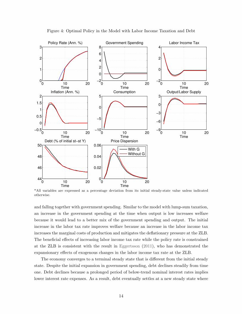
Figure 4: Optimal Policy in the Model with Labor Income Taxation and Debt

0 10 200

1

2

3

Time

Policy Rate (Ann. %)

0 10 20−2

0

2

4

6

8Government Spending

Time0 10 20

−2

0

2

4Labor Income Tax

Time

0 10 20−0.5

0

0.5

1

1.5

2Inflation (Ann. %)

Time0 10 20

−10

−5

0

5Consumption

Time0 10 20

−9

−6

−3

0


Time

0 10 2044

46

48

50Debt (% of initial st−st Y)

Time0 10 20

0

0.02

0.04

0.06Price Dispersion

Time

With G

Without G


and falling together with government spending. Similar to the model with lump-sum taxation,

an increase in the government spending at the time when output is low increases welfare

because it would lead to a better mix of the government spending and output. The initial

increase in the labor tax rate improves welfare because an increase in the labor income tax

increases the marginal costs of production and mitigates the deflationary pressure at the ZLB.

The beneficial effects of increasing labor income tax rate while the policy rate is constrained

at the ZLB is consistent with the result in Eggertsson (2011), who has demonstrated the

expansionary effects of exogenous changes in the labor income tax rate at the ZLB.

The economy converges to a terminal steady state that is different from the initial steady

state. Despite the initial expansion in government spending, debt declines steadily from time

one. Debt declines because a prolonged period of below-trend nominal interest rates implies

lower interest rate expenses. As a result, debt eventually settles at a new steady state where

14

the debt-to-output ratio is lower than that in the initial steady state. Since the debt level is

lower, consumption, output, and government spending are higher, and the labor income tax

rate is lower, in this terminal steady state than in the initial steady state. This is consistent

with the earlier analysis of the Ramsey steady states in section 4.

The initial increase in government spending is modest, about 7 percent of its initial

steady-state level, and is roughly the same as that in the model with lump-sum taxation. As

in the model with lump-sum taxation, a rise in inflation is more subdued with government

spending policy than without it. As a result, price dispersion rises by a smaller amount.

Without access to government spending policy, debt declines by more and converges to a

new steady-state level that is slightly lower than the level where it would converge with the

government spending.

With the size of variations in government spending being roughly the same as in the

model with lump-sum taxation, the welfare implication of government spending policy in

this model is similar to that in the model with lump-sum taxation. As shown in the second

row of table 2, the welfare cost of the ZLB is 1.36 percent with government spending policy

while it is 1.54 percent without it. The welfare gain of government spending policy is about

0.2 percentage points.

5.3 Model with Consumption Tax and Debt

Figure 5 shows the impulse response functions of the model’s key variables in the model

with a consumption tax and debt. Black and red lines are for the unconstrained and the

constrained economies, respectively.

As in the other two models, optimal interest rate policy is characterized by an extended

period of keeping the policy rate at the ZLB. Inflation overshoots while at the ZLB, which

mitigates the initial decline in inflation.

Optimal path of consumption tax is characterized by an initial decline followed by an

overshooting and eventual return to the new steady state. An expected change in the con-

sumption tax affects the household’s intertemporal decision in the same way as the level of

the interest rate affects it. From the consumption Euler equation (11), it can be seen that an

expected increase in the consumption tax rate induces the household to spend more today

and less tomorrow, just as a reduction in the nominal interest does so. As a result, the gov-

ernment can stimulate consumption today by promising to increase the consumption tax rate

in the future. In an environment where the household discount rate is high, the government

finds it optimal to stimulate consumption by reducing the consumption tax rate initially and

raising it afterwards. This consumption tax policy induces the household to even increase

consumption initially.

Optimal government spending policy follows the same pattern as that in the models with

lump-sum taxation and labor income taxation. In this model, consumption is initially higher

than the steady-state level, so the marginal cost of reducing consumption is low. Thus, the

15

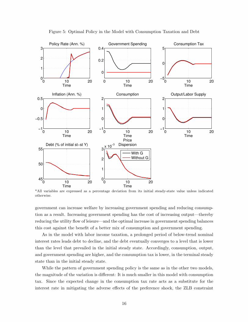
Figure 5: Optimal Policy in the Model with Consumption Taxation and Debt

0 10 200

1

2

3Policy Rate (Ann. %)

Time0 10 20

0

0.2

0.4Government Spending

Time0 10 20

−5

0

5Consumption Tax

Time

0 10 20−1

−0.5

0

0.5Inflation (Ann. %)

Time0 10 20

−1

0

1

2Consumption

Time0 10 20

−1

0

1


Time

0 10 2045

50

55Debt (% of initial st−st Y)

Time0 10 20

0

1

2

3x 10

−3

PriceDispersion

Time

With G

Without G


government can increase welfare by increasing government spending and reducing consump-

tion as a result. Increasing government spending has the cost of increasing output—thereby

reducing the utility flow of leisure—and the optimal increase in government spending balances

this cost against the benefit of a better mix of consumption and government spending.

As in the model with labor income taxation, a prolonged period of below-trend nominal

interest rates leads debt to decline, and the debt eventually converges to a level that is lower

than the level that prevailed in the initial steady state. Accordingly, consumption, output,

and government spending are higher, and the consumption tax is lower, in the terminal steady

state than in the initial steady state.

While the pattern of government spending policy is the same as in the other two models,

the magnitude of the variation is different: It is much smaller in this model with consumption

tax. Since the expected change in the consumption tax rate acts as a substitute for the

interest rate in mitigating the adverse effects of the preference shock, the ZLB constraint

16

on the nominal interest rate is less destabilizing. Consumption and output are much more

stabilized in this model than the other two models. There is not much left for the government

spending policy to contribute.

Reflecting the small variation in government spending in this model, the welfare gain of

government spending policy is small. According to the last row of table 2, the welfare cost of

the ZLB is 0.06 percent with government spending policy while it is 0.07 percent without it.

The welfare gain of optimally choosing government spending is only 0.01 percentage points,

substantially lower than those in the models with lump-sum tax and labor income tax/debt.

5.4 Importance of the Initial Debt Level

Thus far, we have analyzed the economies with a distortionary tax and debt, assuming

a specific initial debt level that is broadly consistent with the debt level in the U.S. a year

before the Great Recession. However, some countries have larger debts than others. I now

discuss how optimal policy depends on the initial debt level.

Model with labor income tax and debt: The top panels of figure 6 show the impulse

response function of government spending, the nominal interest rate, and the labor income tax

rate for the economies with labor income taxation with three alternative initial debt-to-GDP

ratios (0.5, 1.0, 1.5).

According to the figure, the patterns of optimal policies do not depend on the initial debt-

to-output ratio. Optimal government spending policy is characterized by an initial expansion

followed by an undershooting and eventual return to the terminal steady state. Optimal

nominal interest rate policy is characterized by an extended period of keeping the policy rate

at the ZLB. Optimal labor income tax policy is characterized by an initial increase followed

by reduction below, and the eventual return to, the terminal steady state.

While the pattern of optimal government spending policy does not depend on the initial

debt level, the magnitude of variation does. In particular, the initial expansion in government

spending is larger with a higher debt, and government spending converges to a higher level

(relative to the initial steady-state level) when the debt is higher, as shown in the bottom-left

panel of figure 6. This result arises because, given that the nominal interest rate policy is

invariant to the initial debt level, the reduction in the debt from the initial steady state to

the terminal steady state is larger when the initial debt is higher. A reduction in debt means

that the economy is closer to the efficient levels: The tax rate is lower, and consumption,

output, and government spending are higher. Thus, a larger reduction in debt means that the

consumption, output, and government spending increase by more from their initial steady-

state levels.

The welfare gain of government spending policy is larger with a higher initial debt, as

shown in the bottom-middle panel of figure 6. In the model with debt, the government

spending policy not only has short-run stabilization effects, but also the long-run effects on

17

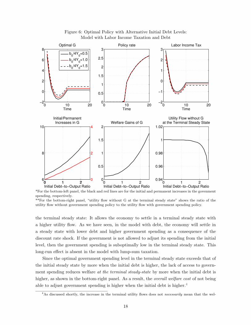
Figure 6: Optimal Policy with Alternative Initial Debt Levels:Model with Labor Income Taxation and Debt

0 10 20−2

0

2

4

6

8Optimal G

Time

b0/4Y

0=0.5

b0/4Y

0=1.0

b0/4Y

0=1.5

0 10 200

0.5

1

1.5

2

2.5

3Policy rate

Time0 10 20

−2

−1

0

1

2

3Labor Income Tax

Time

0 1 26

8

10

Initial Debt−to−Output Ratio

Initial/PermanentIncreases in G

0 1 20

2

4

0 1 20

0.5

1

1.5

2Welfare Gains of G

Initial Debt−to−Output Ratio0 1 2

0.94

0.96

0.98

1

1.02

Utility Flow without Gat the Terminal Steady State


*For the bottom-left panel, the black and red lines are for the initial and permanent increases in the govenmentspending, respectively.**For the bottom-right panel, “utility flow without G at the terminal steady state” shows the ratio of theutility flow without government spending policy to the utility flow with government spending policy.

the terminal steady state: It allows the economy to settle in a terminal steady state with

a higher utility flow. As we have seen, in the model with debt, the economy will settle in

a steady state with lower debt and higher government spending as a consequence of the

discount rate shock. If the government is not allowed to adjust its spending from the initial

level, then the government spending is suboptimally low in the terminal steady state. This

long-run effect is absent in the model with lump-sum taxation.

Since the optimal government spending level in the terminal steady state exceeds that of

the initial steady state by more when the initial debt is higher, the lack of access to govern-

ment spending reduces welfare at the terminal steady-state by more when the initial debt is

higher, as shown in the bottom-right panel. As a result, the overall welfare cost of not being

able to adjust government spending is higher when the initial debt is higher.4

4As discussed shortly, the increase in the terminal utility flows does not necessarily mean that the wel-

18

Model with consumption tax and debt: Figure 7 shows the same set of panels for

the model with a consumption tax and debt.

Figure 7: Optimal Policy with Alternative Initial Debt Levels:Model with Consumption Taxation and Debt

0 10 200

0.3

0.6

0.9

1.2Optimal G

Time

b0/4Y

0=0.5

b0/4Y

0=1

b0/4Y

0=1.5

0 10 200

2

4

6

8Policy rate

Time0 10 20

−8

−6

−4

−2

0

2Consumption Tax

Time

0 1 20

0.2

0.4

0.6

0.8

1

Initial/PermanentIncreases in G


0

0.01

0.02

0.03

0.04

0.05

0.06Welfare Gains of G


0.985

0.99

0.995

1

1.005

Utility Flow without Gat the Terminal Steady State


*For the bottom-left panel, the black and red lines are for the initial and permanent increases in govenmentspending, respectively.**For the bottom-right panel, “utility flow without G at the terminal steady state” shows the ratio of theutility flow without government spending policy to the utility flow with government spending policy.

The patterns of optimal government spending and consumption tax policies are invariant

to the initial debt level. While optimal government spending policy is characterized by the

initial increase followed by the reduction below, and the eventual convergence to, the new

steady state, optimal consumption tax policy is characterized by a mirror image of optimal

government spending path.

The pattern of the nominal interest rate policy is also invariant to the initial debt level

fare gain, as measured by the time-one transfer of consumption as a percentage of the initial steady-stateconsumption, is larger, because the initial steady-state consumptions are different across different initial debtlevels.

19

when the initial debt level is below a certain threshold; the government lowers the policy rate

to zero at time one and keeps it there for an extended period of time. When the debt level

is above that threshold, optimal policy prescribes that the government not lower the policy

rate to the ZLB. This result is obtained because the changes in consumption tax rates acts

as a substitute for the nominal interest rate policy. When the debt level is sufficiently high,

the initial decline in the consumption tax rate is so large and a positive nominal interest

rate is needed to restrain consumption. Consistent with this nominal interest rate policy, the

Lagrange multiplier on the ZLB constraint at time one becomes zero when the initial debt

level is sufficiently high, as shown in figure 8. When the initial debt level is such that optimal

policy rate is positive at time one, the policy rate is higher with a higher initial debt.

The welfare gain of government spending policy varies with the initial debt level in a non

monotonic way, as shown in the bottom-middle panel of figure 7. It increases with the initial

debt level up to a point for the same reason as in the model with a labor income taxation and

debt, namely that the access to government spending policy allows the economy to settle in a

steady state that is more efficient. However, the increase in the terminal utility flows does not

necessarily mean that the welfare gain, as measured by the time-one transfer of consumption

as a percentage of the initial steady-state consumption, is larger, because the initial steady-

state consumptions are different across different initial debt levels. When the initial debt-to-

output ratio is sufficiently high—higher than 1.75 in this parameterization—higher initial debt

is associated with a lower welfare gain of government spending. Nevertheless, for the range

of initial debt levels considered in this paper, even when the initial debt-to-output ratio is

higher than 1.75, the welfare gain of government spending policy remain substantially higher

than that in the baseline parameterization with the initial debt-to-output ratio of 0.5.

5.5 Sensitivity Analyses

Various results shown thus far are robust to alternative values of structural parameters.

For the sake of brevity, the robustness of the results are shown in the appendix.

6 Conclusion

The paper has characterized optimal government spending and monetary policy when

the nominal interest rate is subject to the the ZLB constraint in a sticky-price model. I

departed from the previous literature by analyzing the economies with distortionary taxation

and nominal debt. I have shown that, regardless of the tax instrument, optimal government

spending policy is characterized by an initial expansion followed by a sharp decline below, and

an eventual return to, the steady state. While the pattern of optimal government spending

policy does not depend on the available tax instrument, its magnitude does. In particular,

the amount of variation in government spending is much smaller in the model with a con-

sumption tax than in the model with a labor-income or lump-sum tax. I also documented

20

Figure 8: The Shadow Value of the ZLB Constraintin the Model with Consumption Taxation and Debt

0 2 4 6 8 10 12 14 16 18 200

0.5

1

1.5

2

2.5

3

3.5

Lagrange multiplier

Time

b0/4Y

0=0.75

b0/4Y

0=1

b0/4Y

0=1.25

b0/4Y

0=1.5

that the magnitude of optimal variations in the government spending and the welfare gain

from government spending policy increase with the initial debt level. If the economy starts

with a large initial debt, the welfare gains can be large as the access to government spending

policy improves welfare not only in the short run, but also in the long run.

In this paper, I have broken the Ricardian equivalence by abandoning the lump-sum

tax assumption and introducing a distortionary tax into the model. There are many other

plausible ways in which the Ricardian equivalence may fail in reality, such as the presence of

liquidity-constrained households or the presence of frictions in the labor or financial markets.

Some have recently studied the implications of these frictions for fiscal multipliers at the

ZLB.5 It would be useful to study their implications for optimal government spending policy

in future research.6

References

Adam, K. (2011): “Government Debt and Optimal Monetary and Fiscal Policy,” European Economic

Review, 55, 57–74.

5For example, Carrillo and Poilly (2013) analyze the government spending multiplier in a model withfinancial frictions. Roulleau-Pasdeloup (2014) examines the government spending multiplier in a model withsearch and matching frictions in the labor market.

6Bilbiie, Monacelli, and Perotti (2014) study the welfare effects of exogenous changes in governmentspending in the model where a fraction of households do not have access to the bond market.

21

Benigno, P., and M. Woodford (2004): “Optimal Monetary and Fiscal Policy: A Linear

Quadratic Approach,” NBER Macroeconomics Annual 2003, 18, 271–333.

Bilbiie, F. O., T. Monacelli, and R. Perotti (2014): “Is Government Spending at the Zero

Lower Bound Desirable?,” NBER Working Paper No. 20687.

Burgert, M., and S. Schmidt (2014): “Dealing with a liquidity trap when government debt

matters: Optimal time-consistent monetary and fiscal policy,” Journal of Economic Dynamics and

Control, 47, 282–299.

Carrillo, J. A., and C. Poilly (2013): “How Do Financial Frictions Affect the Spending Multiplier

During a Liquidity Trap?,” Review of Economic Dynamics, 16(2), 296–311.

Christiano, L., M. Eichenbaum, and S. Rebelo (2011): “When is the Government Spending

Multiplier Large?,” Journal of Political Economy, 119(1), 78–121.

Correia, I. H., E. Farhi, J. P. Nicolini, and P. Teles (2013): “Unconventional Fiscal Policy

at the Zero Bound,” American Economic Review, 103(4), 1172–1211.

Eggertsson, G. (2011): “What Fiscal Policy is Effective at Zero Interest Rates?,” NBER Macroe-

conomic Annual 2010, 25, 59–112.

Eggertsson, G., and M. Woodford (2004): “Optimal Monetary and Fiscal Policy in a Liquidity

Trap,” NBER International Seminar on Macroeconomics, pp. 75–144.

Juillard, M., D. Laxton, P. McAdam, and H. Pioro (1998): “An algorithm competition: First-

order iterations versus Newton-based techniques,” Journal of Economic Dynamics and Control,

22(8-9), 1291–1318.

Khan, A., R. King, and A. Wolman (2003): “Optimal Monetary Policy,” Review of Economic

Studies, 70(4), 825–860.

Leith, C., I. Moldovan, and R. Rossi (2015): “Monetary and Fiscal Policy under Deep Habits,”

Working Paper, 52, 55–74.

Leith, C., and S. Wren-Lewis (2013): “Fiscal Sustainability in a New Keynesian Model,” Journal

of Money, Credit and Banking, 45(8), 1477–1516.

Levin, A., D. Lopez-Salido, E. Nelson, and T. Yun (2010): “Limitations on the Effectiveness

of Forward Guidance at the Zero Lower Bound,” International Journal of Central Banking, 6(1),

143–189.

Mateev, D. (2014): “Time-Consistentnsistent Management of a Liquidity Trap: Monetary and Fiscal

Policy with Debt,” Mimeo.

Motta, G., and R. Rossi (2014): “Ramsey Monetary and Fiscal Policy: the Role of Consumption

Taxation,” Working Paper.

Nakata, T. (2013a): “Optimal Fiscal and Monetary Policy With Occasionally Binding Zero Bound

Constraints,” Finance and Economics Discussion Series 2013-40, Board of Governors of the Federal

Reserve System (U.S.).

22

(2013b): “Uncertainty at the Zero Lower Bound,” Finance and Economics Discussion Series

2013-09, Board of Governors of the Federal Reserve System (U.S.).

Roulleau-Pasdeloup, J. (2014): “The Government Spending Multiplier in a Recession with a

Binding Zero Lower Bound,” Mimeo.

Schmidt, S. (2013): “Optimal Monetary and Fiscal Policy with a Zero Bound on Nominal Interest

Rates,” Journal of Money, Credit and Banking, 45(7), 1335–1350.

Schmitt-Grohe, S., and M. Uribe (2004): “Optimal fiscal and monetary policy under sticky

prices,” Journal of Economic Theory, 114(2), 198–230.

Siu, H. E. (2004): “Optimal fiscal and monetary policy with sticky prices,” Journal of Monetary

Economics, 51(3), 575–607.

Werning, I. (2012): “Managing a Liquidity Trap: Monetary and Fiscal Policy,” Working Paper.

Woodford, M. (2011): “Simple Analytics of the Government Expenditure Multiplier,” American

Economic Journal: Macroeconomics, 3(1), 1–35.

23

Appendices

Appendix A demonstrates the robustness of key results in the main text to alternative valuesof key structural parameters. Appendix B explains the solution method. Appendix C presentsthe Lagrangean problem of the government and its first-order necessary conditions.

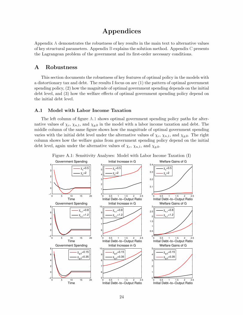
A Robustness

This section documents the robustness of key features of optimal policy in the models witha distortionary tax and debt. The results I focus on are (1) the pattern of optimal governmentspending policy, (2) how the magnitude of optimal government spending depends on the initialdebt level, and (3) how the welfare effects of optimal government spending policy depend onthe initial debt level.

A.1 Model with Labor Income Taxation

The left column of figure A.1 shows optimal government spending policy paths for alter-native values of χc, χn,1, and χg,0 in the model with a labor income taxation and debt. Themiddle column of the same figure shows how the magnitude of optimal government spendingvaries with the initial debt level under the alternative values of χc, χn,1, and χg,0. The rightcolumn shows how the welfare gains from government spending policy depend on the initialdebt level, again under the alternative values of χc, χn,1, and χg,0.

Figure A.1: Sensitivity Analyses: Model with Labor Income Taxation (I)

0 5 10 15 20−1

0

1

2

3

4

Government Spending

Time

χc=0.5

χc=2

0 0.5 1 1.5 2 2.50

1

2

3

4

5

6

Initial Increase in G


χc=0.5

χc=2

0 0.5 1 1.5 2 2.50

0.1

0.2

0.3

0.4

Welfare Gains of G


χc=0.5

χc=2

0 5 10 15 20−2

0

2

4

6

8

Government Spending

Time

χn,1

=0.8

χn,1

=1.2

0 0.5 1 1.5 2 2.55

6

7

8

9

10



χn,1

=0.8

χn,1

=1.2

0 0.5 1 1.5 2 2.50

0.5

1

1.5

2

2.5

3

Welfare Gains of G


χn,1

=0.8

χn,1

=1.2

0 5 10 15 20−2

0

2

4

6

8

Government Spending

Time

χg,0

=0.15

χg,0

=0.35

0 0.5 1 1.5 2 2.55

6

7

8

9

10



χg,0

=0.15

χg,0

=0.35

0 0.5 1 1.5 2 2.50

1

2

3

4

5

Welfare Gains of G


χg,0

=0.15

χg,0

=0.35

24

The left column of figure A.2 shows optimal government spending policy paths for alter-native values of χg,1, θ, and α in the model with a labor income taxation and debt. Themiddle column of the same figure shows how the magnitude of optimal government spendingvaries with the initial debt level under the alternative values of χg,1, θ, and α. The rightcolumn shows how the welfare gains from government spending policy depend on the initialdebt level under the alternative values of χg,1, θ, and α.

Figure A.2: Sensitivity Analyses: Model with Labor Income Taxation (II)

0 5 10 15 20−5

0

5

10

Government Spending

Time

χg,1

=0.8

χg,1

=1.2

0 0.5 1 1.5 2 2.54

6

8

10

12



χg,1

=0.8

χg,1

=1.2

0 0.5 1 1.5 2 2.50

1

2

3

4

Welfare Gain of G


χg,1

=0.8

χg,1

=1.2

0 5 10 15 20−2

0

2

4

6

8

Government Spending

Time

θ=5

θ=15

0 0.5 1 1.5 2 2.54

5

6

7

8

9

10



θ=5

θ=15

0 0.5 1 1.5 2 2.50

0.5

1

1.5

2

2.5

3

Welfare Gain of G


θ=5

θ=15

0 5 10 15 20−5

0

5

10

Government Spending

Time

α=0.6α=0.9

0 0.5 1 1.5 2 2.52

4

6

8

10

12



α=0.6α=0.9

0 0.5 1 1.5 2 2.50

0.5

1

1.5

2

Welfare Gain of G


α=0.6α=0.9

According to the left columns of these two figures, optimal government spending policy ischaracterized by the initial increase, followed by the reduction below, and the eventual returnto, the new steady state, regardless of the parameter values. The middle columns of these twofigures demonstrate the robustness of the result that the initial increase in the governmentspending is larger when the initial debt is larger. Finally, the right columns show that thewelfare gain of government spending policy increases with the initial debt level, regardless ofthe parameter values.

A.2 Model with Consumption Taxation

The left column of figure A.4 shows optimal government spending policy paths for alter-native values of χc, χn,1, and χg,0 in the model with a consumption taxation and debt. Themiddle column of the same figure shows how the magnitude of optimal government spendingvaries with the initial debt level under the alternative values of χc, χn,1, and χg,0. The rightcolumn shows how the welfare gains from government spending policy depend on the initialdebt level, again under the alternative values of χc, χn,1, and χg,0.

25

Figure A.3: Sensitivity Analyses: Model with Consumption Taxation (I)

0 5 10 15 20−1

−0.5

0

0.5

1

1.5

Government Spending

Time

χc=0.5

χc=2

0 0.5 1 1.5 2 2.50.4

0.6

0.8

1

1.2

1.4



χc=0.5

χc=2

0 0.5 1 1.5 2 2.50

0.005

0.01

0.015

0.02

0.025

0.03

Welfare Gains of G


χc=0.5

χc=2

0 5 10 15 20−0.2

0

0.2

0.4

0.6

Government Spending

Time

χn,1

=0.8

χn,1

=1.2

0 0.5 1 1.5 2 2.50

0.2

0.4

0.6

0.8

1



χn,1

=0.8

χn,1

=1.2

0 0.5 1 1.5 2 2.50

0.02

0.04

0.06

0.08

Welfare Gains of G


χn,1

=0.8

χn,1

=1.2

0 5 10 15 20−0.2

0

0.2

0.4

0.6

Government Spending

Time

χg,0

=0.15

χg,0

=0.35

0 0.5 1 1.5 2 2.50

0.2

0.4

0.6

0.8

1



χg,0

=0.15

χg,0

=0.35

0 0.5 1 1.5 2 2.50

0.02

0.04

0.06

0.08

0.1

0.12

Welfare Gains of G


χg,0

=0.15

χg,0

=0.35

The left column of figure A.3 shows optimal government spending policy paths for alter-native values of χg,1, θ, and α in the model with a consumption taxation and debt. Themiddle column of the same figure shows how the magnitude of optimal government spendingvaries with the initial debt level under the alternative values of χg,1, θ, and α. The rightcolumn shows how the welfare gains from government spending policy depend on the initialdebt level under the alternative values of χg,1, θ, and α.

According to the left columns of these two figures, optimal government spending policy ischaracterized by the initial increase, followed by the reduction below, and the eventual returnto, the new steady state, regardless of the parameter values. The middle columns of these twofigures demonstrate the robustness of the result that the initial increase in the governmentspending is larger when the initial debt is larger. Finally, the right columns show that thewelfare gain of government spending policy increases with the initial debt level unless theinitial debt is sufficiently large, regardless of the parameter values. However, when the initialdebt level is sufficiently large, the welfare gains decrease with the initial debt level as in thebaseline parameterization of the model with consumption tax.

26

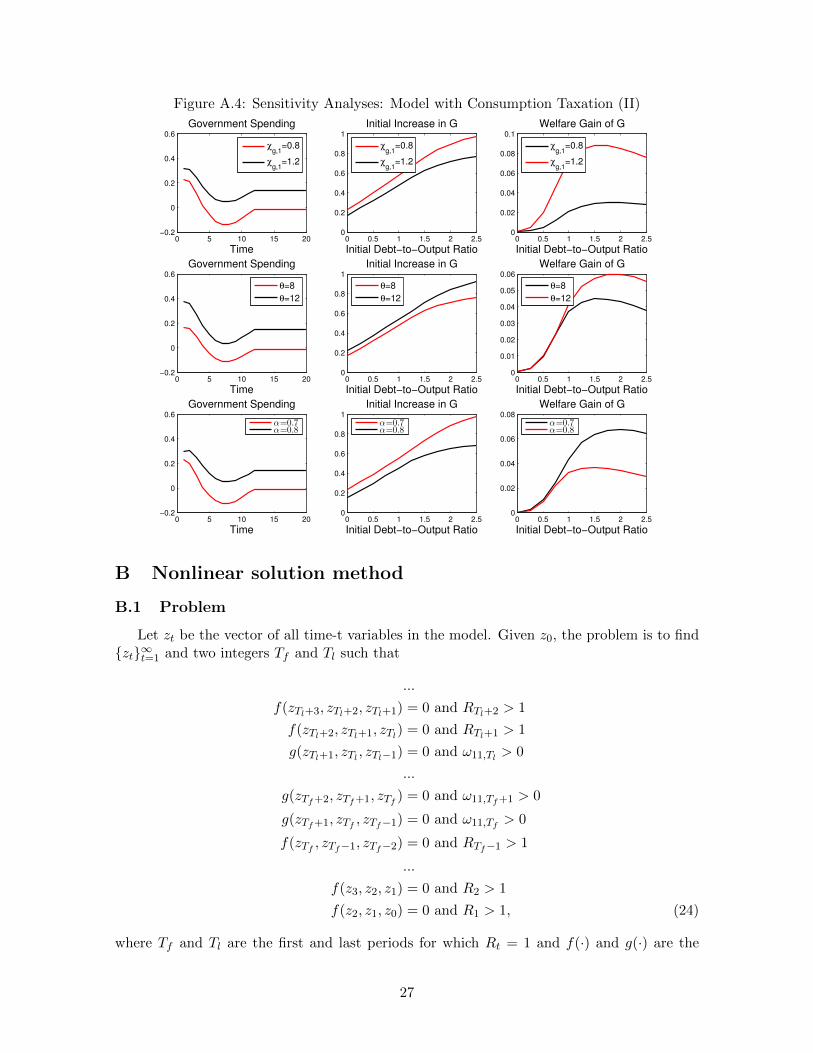
Figure A.4: Sensitivity Analyses: Model with Consumption Taxation (II)

0 5 10 15 20−0.2

0

0.2

0.4

0.6

Government Spending

Time

χg,1

=0.8

χg,1

=1.2

0 0.5 1 1.5 2 2.50

0.2

0.4

0.6

0.8

1



χg,1

=0.8

χg,1

=1.2

0 0.5 1 1.5 2 2.50

0.02

0.04

0.06

0.08

0.1

Welfare Gain of G


χg,1

=0.8

χg,1

=1.2

0 5 10 15 20−0.2

0

0.2

0.4

0.6

Government Spending

Time

θ=8

θ=12

0 0.5 1 1.5 2 2.50

0.2

0.4

0.6

0.8

1



θ=8

θ=12

0 0.5 1 1.5 2 2.50

0.01

0.02

0.03

0.04

0.05

0.06

Welfare Gain of G


θ=8

θ=12

0 5 10 15 20−0.2

0

0.2

0.4

0.6

Government Spending

Time

α=0.7α=0.8

0 0.5 1 1.5 2 2.50

0.2

0.4

0.6

0.8

1



α=0.7α=0.8

0 0.5 1 1.5 2 2.50

0.02

0.04

0.06

0.08

Welfare Gain of G


α=0.7α=0.8

B Nonlinear solution method

B.1 Problem

Let zt be the vector of all time-t variables in the model. Given z0, the problem is to find{zt}∞t=1 and two integers Tf and Tl such that

...

f(zTl+3, zTl+2, zTl+1) = 0 and RTl+2 > 1

f(zTl+2, zTl+1, zTl) = 0 and RTl+1 > 1

g(zTl+1, zTl , zTl−1) = 0 and ω11,Tl > 0

...

g(zTf+2, zTf+1, zTf ) = 0 and ω11,Tf+1 > 0

g(zTf+1, zTf , zTf−1) = 0 and ω11,Tf > 0

f(zTf , zTf−1, zTf−2) = 0 and RTf−1 > 1

...

f(z3, z2, z1) = 0 and R2 > 1

f(z2, z1, z0) = 0 and R1 > 1, (24)

where Tf and Tl are the first and last periods for which Rt = 1 and f(·) and g(·) are the

27

vectors of functions containing the first-order necessary conditions of the Lagrangean problemwhen Rt > 1 and Rt = 1, respectively. f(·) and g(·) are identical except for the last element;the last elements of f(·) and g(·) are ω11,t and Rt − 1, respectively.

In order to reduce the problem into a finite problem, I assume that the economy willhave converged to a terminal Ramsey steady state, ztss, after t=S for some large integer S.The problem then becomes that of finding {zt}St=1, two integers, Tf and Tl, and the terminalRamsey steady state, ztss, such that

f(ztss, ztss, zS) = 0 and RS+1 > 1

f(ztss, zS , zS−1) = 0 and RS > 1

f(zS , zS−1, zS−2) = 0 and RS−1 > 1

...

f(zTl+2, zTl+1, zTl) = 0 and RTl+1 > 1

g(zTl+1, zTl , zTl−1) = 0 and ω11,Tl > 0

...

g(zTf+2, zTf+1, zTf ) = 0 and ω11,Tf+1 > 0

g(zTf+1, zTf , zTf−1) = 0 and ω11,Tf > 0

f(zTf , zTf−1, zTf−2) = 0 and RTf−1 > 1

...

f(z3, z2, z1) = 0 and R2 > 1

f(z2, z1, z0) = 0 and R1 > 1. (25)

B.2 Solution Method: A Big Picture

I use the “Newton-within-Shooting” algorithm to solve this problem. The algorithmproceeds as follows.

• Step 1: Guess Tf and Tl

– Step 1.A: Guess btss, a level of debt at the terminal steady state.

– Step 1.B: Compute ztss, the terminal Ramsey steady state, associated with btss.

– Step 1.C: Given ztss, use the modified Newton algorithm described below to solvefor {zt}St=1.

– Step 1.D: Check the first-order necessary conditions at t = S + 1 are satisfied. Ifnot, adjust the debt level at the terminal Ramsey steady state and go back to Step1.B.

• Step 2: Check if ω11,t ≥ 0 and Rt ≥ 1 for all 1 ≤ t ≤ S. If not, adjust Tf and Tl and goback to Step 1.

The Newton algorithm I use in step 1.C is the modified Newton method of Juillard, Laxton,McAdam, and Pioro (1998), which I shall describe shortly. Given Tf , Tl, and ztss, the goal of

28

the modified Newton algorithm is to find {zt}St=1 satisfying the equilibrium conditions fromt = 1 to t = S. The number of equations is the same as the number of variables.7

B.3 Modified Newton Algorithm

By stacking zt into a vector Y = [z′1, z′2, ..., z

′S−1, z

′S ]′, we can express the problem as that

of finding Y such thatF (Y ) = 0, (26)

where F (·) is a vector of functions stacking f(·) and g(·) from t = 1 to t = S. As in anyNewton algorithm, we start by an initial guess of Y, Y (1). At a k-th iteration, given aprevious guess Y (k), I compute an adjustment factor ∆Y by solving the following system oflinear equations: [∂F (Y )

∂Y

]Y (k)

∆Y = −F (Y (k)). (27)

If ||∆Y || < εtol, the algorithm ends. Otherwise, I set our next guess of Y as

Y (k+1) = Y (k) + µ∆Y (28)

I set µ = 0.5 and εtol = 10e− 15.When the system of equations is small, we can find the ∆Y that satisfies equation (27)

by inverting[∂F (Y )∂Y

]Y (k)

. However, when the system is large, inverting this matrix is compu-

tationally costly. Juillard, Laxton, McAdam, and Pioro (1998) proposed to solve for ∆Y inequation (27) by making use of the sparseness of the matrix, which comes from the recursivestructure of the problem.

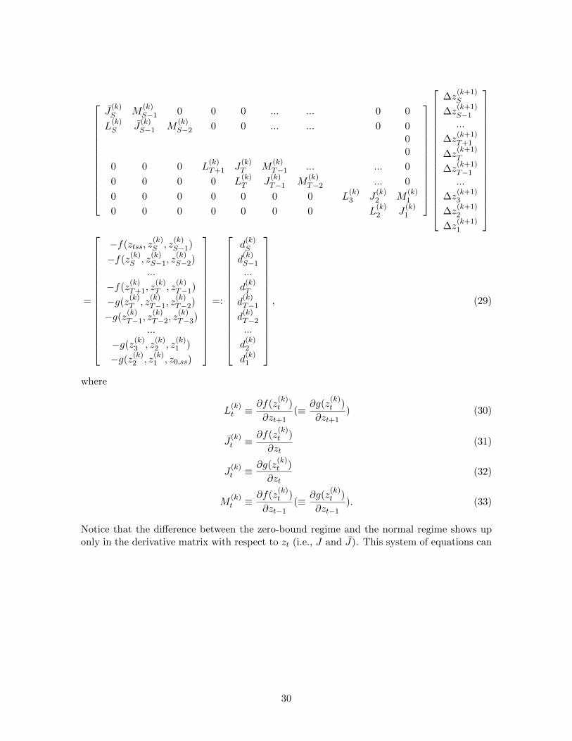
I now turn to the details of their algorithm. For the clarity of exposition, I focus on thecase where the the zero lower bound binds initially (i.e., Tf = 0) in what follows. Equation(27) can be written as

7While I have not been able to prove the uniqueness of the solution, this Newton algorithm returns theunique solution regardless of the starting values used to initiate the algorithm.

29

J(k)S M

(k)S−1 0 0 0 ... ... 0 0

L(k)S J

(k)S−1 M

(k)S−2 0 0 ... ... 0 0

00

0 0 0 L(k)T+1 J

(k)T M

(k)T−1 ... ... 0

0 0 0 0 L(k)T J

(k)T−1 M

(k)T−2 ... 0

0 0 0 0 0 0 0 L(k)3 J

(k)2 M

(k)1

0 0 0 0 0 0 0 L(k)2 J

(k)1

∆z(k+1)S

∆z(k+1)S−1...

∆z(k+1)T+1

∆z(k+1)T

∆z(k+1)T−1...

∆z(k+1)3

∆z(k+1)2

∆z(k+1)1

=

−f(ztss, z(k)S , z

(k)S−1)

−f(z(k)S , z

(k)S−1, z

(k)S−2)

...

−f(z(k)T+1, z

(k)T , z

(k)T−1)

−g(z(k)T , z

(k)T−1, z

(k)T−2)

−g(z(k)T−1, z

(k)T−2, z

(k)T−3)

...

−g(z(k)3 , z

(k)2 , z

(k)1 )

−g(z(k)2 , z

(k)1 , z0,ss)

=:

d(k)S

d(k)S−1...

d(k)T

d(k)T−1d(k)T−2...

d(k)2

d(k)1

, (29)

where

L(k)t ≡

∂f(z(k)t )

∂zt+1(≡ ∂g(z

(k)t )

∂zt+1) (30)

J(k)t ≡ ∂f(z

(k)t )

∂zt(31)

J(k)t ≡ ∂g(z

(k)t )

∂zt(32)

M(k)t ≡ ∂f(z

(k)t )

∂zt−1(≡ ∂g(z

(k)t )

∂zt−1). (33)

Notice that the difference between the zero-bound regime and the normal regime shows uponly in the derivative matrix with respect to zt (i.e., J and J). This system of equations can

30

also be written as

J(k)S ∆z

(k+1)S +M

(k)S−1∆z

(k+1)S−1 = d

(k)S

L(k)S ∆z

(k+1)S + J

(k)S−1∆z

(k+1)S−1 +M

(k)S−2∆z

(k+1)S−2 = d

(k)S−1

...

L(k)T+2∆z

(k+1)T+2 + J

(k)T+1∆z

(k+1)T+1 +M

(k)T ∆z

(k+1)T+1 = d

(k)T+1

L(k)T+1∆z

(k+1)T+1 + J

(k)T ∆z

(k+1)T +M

(k)T−1∆z

(k+1)T = d

(k)T

L(k)T ∆z

(k+1)T + J

(k)T−1∆z

(k+1)T−1 +M

(k)T−2∆z

(k+1)T−2 = d

(k)T−1

...

L(k)3 ∆z

(k+1)3 + J

(k)2 ∆z

(k+1)2 +M

(k)1 ∆z

(k+1)1 = d

(k)2

L(k)2 ∆z

(k+1)2 + J

(k)1 ∆z

(k+1)1 = d

(k)1 . (34)

Notice that finding ∆Y in equation (27) is equivalent to finding a sequence of {∆z(k+1)t }St=1

that satisfies this system.

To find {∆z(k+1)t }St=1, notice that

∆z(k+1)S =

[J(k)S

]−1d(k)S −

[J(k)S

]−1M

(k)S−1∆z

(k+1)S−1

= Λ(k)S + Φ

(k)S ∆z

(k+1)S−1 . (35)

Plugging this into the equation for t = S − 1, I obtain

L(k)S [Λ

(k)S + Φ

(k)S ∆z

(k+1)S−1 ] + J

(k)S−1∆z

(k+1)S−1 +M

(k)S−2∆z

(k+1)S−2 = d

(k)S−1 (36)

⇒

∆z(k+1)S−1 =

[L(k)S Φ

(k)S + J

(k)S−1

]−1[d(k)S−1 − L

(k)S Λ

(k)S

]−[L(k)S Φ

(k)S + J

(k)S−1

]−1M

(k)S−2∆z

(k+1)S−2

= Λ(k)S−1 + Φ

(k)S−1∆z

(k+1)S−2 . (37)

This process can be repeated until t = 1. The outcome of this process is the following law ofmotion for ∆zt:

∆z(k+1)S = Λ

(k)S + Φ

(k)S ∆z

(k+1)S−1

∆z(k+1)S−1 = Λ

(k)S−1 + Φ

(k)S−1∆z

(k+1)S−2

...

∆z(k+1)T+1 = Λ

(k)T+1 + Φ

(k)T+1∆z

(k+1)T

∆z(k+1)T = Λ

(k)T + Φ

(k)T ∆z

(k+1)T−1

...

∆z(k+1)2 = Λ

(k)2 + Φ

(k)2 ∆z

(k+1)1

∆z(k+1)1 = Λ

(k)1 , (38)

where the time-varying coefficients are computed recursively as follows:

31

Λ(k)S =

[J(k)S

]−1d(k)S

Φ(k)S = −

[J(k)S

]−1M

(k)S−1

Λ(k)S−1 =

[L(k)S Φ

(k)S + J

(k)S−1

]−1[d(k)S−1 − L

(k)S Λ

(k)S

]Φ(k)S−1 = −

[L(k)S Φ

(k)S + J

(k)S−1

]−1M

(k)S−2

...

Λ(k)T+1 =

[L(k)T+1Φ

(k)T+2 + J

(k)T

]−1[d(k)T − L

(k)T+1Λ

(k)T+2

]Φ(k)T+1 = −

[L(k)T+1Φ

(k)T+2 + J

(k)S−1

]−1M

(k)T−1

Λ(k)T =

[L(k)T Φ

(k)S + J

(k)T−1

]−1[d(k)S−1 − L

(k)S Λ

(k)T+1

]Φ(k)T = −

[L(k)T Φ

(k)S + J

(k)T−1

]−1M

(k)S−2

...

Λ(k)2 =

[L(k)3 Φ

(k)3 + J

(k)2

]−1[d(k)2 − L

(k)3 Λ

(k)3

]Φ(k)2 = −

[L(k)3 Φ

(k)3 + J

(k)2

]−1M

(k)1

Λ(k)1 =

[L(k)2 Φ

(k)2 + J

(k)1

]−1[d(k)1 − L

(k)2 Λ

(k)2

]. (39)

The knowledge of Lt, Jt, Jt, and Mt is sufficient for us to compute these time-varying coeffi-cients given in the set of equations (39). Once the coefficients are computed, one can use the

law of motion given in the set of equations (38) to find the sequence of {∆z(k+1)t }St=1.

32

C The Lagrangean Problem

The Lagrangean problem of the government is given by

L(b0, s0, ω1,0, ω6,0, ω7,0) =

min{ωt}∞t=1max{ut}∞t=1

∞∑t=1

βt−1t−1∏s=0

δs

[C1−χct

1− χc− χn,0

N1+χn,1t

1 + χn,1+ χg,0

G1−χg,1t

1− χg,1

]−ω1,0C

−χc1 Π−11 − ω6,0ζpΠ

θ1Cn,1 − ω7,0ζpΠ

θ−11 Cd,1

+∞∑t=1

βt−1t−1∏s=0

δs

[ω1,t[

C−χct

(1 + τc,t)Rt− βδt

C−χct+1 Π−1t+1

1 + τc,t+1]

+ω2,t[1− τn,t1 + τc,t

wt − χn,0Nχn,1t Cχct ]

+ω3,t[st − (1− ζp)[p∗t]−θ − ζpΠθ

t st−1]

+ω4,t[1− (1− ζp)[p∗t]1−θ − ζpΠθ−1

t ]

+ω5,t[p∗t −

θ

θ − 1

Cn,tCd,t

]

+ω6,t

[Cn,t −

1− νt1 + τc,t

YtwtC−χct − ζpβδtΠθ

t+1Cn,t+1

]+ω7,t

[Cd,t −

1

1 + τc,tYtC

−χct − ζpβδtΠθ−1

t+1Cd,t+1

]+ω8,t[Ytst −Nt]

+ω9,t[Yt − Ct −Gt]+ω10,tGBCt

+ω11,t[Rt − 1]

], (40)

where the problem is indexed by ω1,0, ω6,0, ω7,0 in addition to b0 and s0. The first-ordernecessary conditions of this problem is given by

Ct : C−χct − ω1,tχcC−χc−1t

(1 + τc,t)Rt+ ω1,t−1χc

C−χc−1t Π−1t1 + τc,t

− ω2,tχcχn,0Nχn,1t Cχc−1t

+ ω6,tχcYtwtC

−χc−1t

1 + τc,t+ ω7,tχc

YtC−χc−1t

1 + τc,t− ω9,t − ω10,tτc,t = 0 (41)

Yt : −ω6,twtC

−χct

1 + τc,t− ω7,t

C−χct

1 + τc,t+ ω8,tst + ω9,t = 0 (42)

Nt : −χn,0Nχn,1t − ω2,tχn,1χn,0N

χn,1−1t Cχct − ω8,t − ω10,tτn,twt = 0 (43)

wt : ω2,t1− τn,t1 + τc,t

− ω6,t1− νt1 + τc,t

YtC−χct − ω10,tτn,tNt = 0 (44)

33

Πt : ω1,t−1C−χct Π−2t − ω3,tθζpΠ

θ−1t st−1 − ω4,t(θ − 1)ζpΠ

θ−2t

− ω6,t−1θζpΠθ−1t Cn,t − ω7,t−1(θ − 1)ζpΠ

θ−2t Cd,t = 0 (45)

st : ω3,t − ω3,t+1βδtζpΠθt+1 + ω8,tYt − ω10,tbt−1Π

−2t = 0 (46)

p∗t : ω3,tθ(1− ζp)[p∗t]−θ−1

+ ω4,t(θ − 1)(1− ζp)[p∗t]−θ

+ ω5,t = 0 (47)

Cn,t : −ω5,tθ

θ − 1

1

Cd,t+ ω6,t − ω6,t−1ζpΠ

θt = 0 (48)

Cd,t : ω5,tθ

θ − 1Cn,tC

−2d,t + ω7,t − ω7,t−1ζpΠ

θ−1t = 0 (49)

Rt : −ω1,tC−χct Π−1t R−2t + ω10,tR

−2t bt + ω11,t = 0 (50)

ω11,t = 0 if Rt > 1, ω11,t > 0 if Rt = 1 (51)

Gt : χg,0G−χg,1t − ω9,t + ω10,t = 0 (52)

τc,t : −ω1,t(1 + τc,t)−2C−χct + ω1,t−1(1 + τc,t)

−2C−χct−1

− ω2,t(1 + τc,t)−2wt + ω6,t(1 + τc,t)

−2YtwtC−χct

+ ω7,t(1 + τc,t)−2YtC

−χct − ω10,tCt = 0 (53)

τn,t : −ω2,t1

1 + τc,twt − ω10,twtNt = 0 (54)

bt : −ω10,tR−1t + ω10,t+1βδtΠ

−1t+1 = 0 (55)

Tt : −ω10,t = 0 (56)

as well as the equations characterizing the equilibrium of the model shown in section 2.

34

Optimal Government Spending at the Zero Lower Bound: A Non ...

Documents

Transcript of Optimal Government Spending at the Zero Lower Bound: A Non ...