IESE Business School-University of Navarra - 1

OPTIMAL EXPEDITING DECISIONS IN A CONTINUOUS-STAGE SERIAL SUPPLY CHAIN

Peter Berling

Víctor Martínez-de-Albéniz

IESE Business School – University of Navarra Av. Pearson, 21 – 08034 Barcelona, Spain. Phone: (+34) 93 253 42 00 Fax: (+34) 93 253 43 43 Camino del Cerro del Águila, 3 (Ctra. de Castilla, km 5,180) – 28023 Madrid, Spain. Phone: (+34) 91 357 08 09 Fax: (+34) 91 357 29 13 Copyright © 2011 IESE Business School.

Working Paper

WP-906

February, 2011

Optimal Expediting Decisions in a Continous-Stage Serial Supply Chain

levels. The same type of solution also applies in production environments, as one could increase

the amount of production capacity temporarily to increase throughput and prevent customer

backlogs.

The objective of this paper is precisely to optimize these expediting decisions. This problem

has been studied in the literature before and has been tackled using periodic-review multi-

echelon inventory models. In these models, expediting is modeled by allowing units to be

instantaneously sent from an installation to a lower one, at a cost. Typically, it is found that

the optimal policy is to choose to expedite inventory up-to a given level. This is similar to using

an echelon base-stock policy with a different base-stock level for normal and express modes.

In this paper, we formulate the expediting problem in a continuous setting, under Poisson

demand. We consider a continuous-stage serial supply chain and as a result, the supply chain

manager is allowed to take real-time, continuous production/transportation decisions. In many

aspects, this allows for greater modeling flexibility compared to previous research. Our setting

implies that each inventory unit is located in an infinite rather than a finite set of positions.

For each unit, one can choose at which speed it should be moved downstream, given the state

of the system (and in particular, given how many units are located downstream, closer to

the customer). We can hence optimize total supply chain costs including back-ordering costs,

inventory holding costs that may depend on the location where inventory is standing, and

moving costs that depend both on the location and the speed at which a unit is being moved.

Hence, by choosing the appropriate inventory and transportation costs, our model can mimic

most real systems.

For example, consider the transportation problem of a logistics provider that manages ships

carrying a single product from a port in Northern Europe to a port in China. The company

is in charge of serving customers at the destination, and hence will send/dispatch ships as

demand arrives. In addition, if demand is temporarily high, it can choose to increase the speed

of the ships in order to avoid back-ordering costs. However, due to the costs involved with

faster transportation, the company must know when this option makes sense, and delivery is

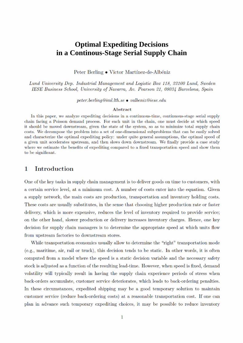
sufficiently “urgent”. Figure 1 shows the fuel consumption of ships as a function of speed. One

can see that, if the current level of inventory downstream is sufficient, the company will be better

off setting a low speed, in order to reduce transportation cost. On the other hand, if current

inventory is too low, then it will choose to set a higher speed, thus increasing transportation

cost but reducing expected back-ordering charges.

Our model thus allows us to optimize such decisions in a continuous setting. We formulate

the problem as an optimal control problem. Observing that orders should never cross at opti-

mality, we decompose the problem into a set of one-dimensional subproblems that can be easily

2

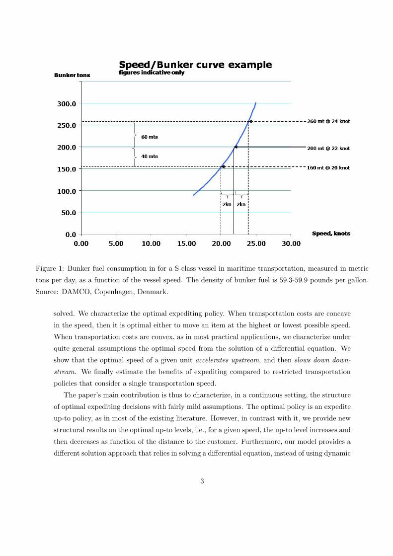
Figure 1: Bunker fuel consumption in for a S-class vessel in maritime transportation, measured in metric

tons per day, as a function of the vessel speed. The density of bunker fuel is 59.3-59.9 pounds per gallon.

Source: DAMCO, Copenhagen, Denmark.

solved. We characterize the optimal expediting policy. When transportation costs are concave

in the speed, then it is optimal either to move an item at the highest or lowest possible speed.

When transportation costs are convex, as in most practical applications, we characterize under

quite general assumptions the optimal speed from the solution of a differential equation. We

show that the optimal speed of a given unit accelerates upstream, and then slows down down-

stream. We finally estimate the benefits of expediting compared to restricted transportation

policies that consider a single transportation speed.

The paper’s main contribution is thus to characterize, in a continuous setting, the structure

of optimal expediting decisions with fairly mild assumptions. The optimal policy is an expedite

up-to policy, as in most of the existing literature. However, in contrast with it, we provide new

structural results on the optimal up-to levels, i.e., for a given speed, the up-to level increases and

then decreases as function of the distance to the customer. Furthermore, our model provides a

different solution approach that relies in solving a differential equation, instead of using dynamic

3

programming. This allows us to provide insights on the sensitivity of the optimal policy and

cost to the cost parameters. Finally, we present a case study on the shipping problem described

above. We evaluate the impact of having the possibility of adjusting the speed dynamically at

4.5%, which is significant for the industry. We also discuss the influence of the price of fuel on

fuel consumption, and provide quantitative estimates of the potential effectiveness of fuel taxes

for emissions reduction. Interestingly, this complements a report by the World Economic Forum

[21] where “despeeding the supply chain” has been identified as one of the main opportunities

to reduce CO2 emissions.

The rest of the paper is organized as follows. §2 reviews the literature on multi-echelon

inventory management and in particular on expediting. We then describe the model in §3 and

formulate the optimization problem. In §4 we characterize the optimal expediting policy. We

provide sensitivity analysis and a case study on maritime shipping in §5. We conclude the

paper in §6. All the proofs are included in the appendix.

2 Literature Review

First of all, the approach used in this paper is to decompose a complex inventory problem

into unit-by-unit subproblems. This methodology was pioneered by Axsater [2], and has been

recently used by Muharremoglu and Tsitsiklis [18], Martınez-de-Albeniz and Lago [15], Berling

and Martınez-de-Albeniz [5], Janakiraman and Muckstadt [11] or Yu and Benjaafar [22] among

others. We apply this solution approach to a multi-echelon inventory control problem with

expediting.

The problem that we tackle can be seen as an extension to the seminal work of Clark

and Scarf [8] on multi-echelon inventory management. Indeed, the continuous supply chain

considered here can be seen as a serial system where the number of stages is infinite. Clark and

Scarf introduced the notion of echelon-stock and showed optimality of an echelon base-stock

policy for a finite horizon problem (albeit in the system they considered the same result can be

obtained with an installation-stock policy, see Axsater and Rosling [4]). Federgruen and Zipkin

[9] extended the result to infinite horizons and Chen and Zheng [7] presented an alternative

streamlined proof that is also valid in continuous time. Optimality of an echelon base-stock

policy is a result that carries over to several other systems including some of the scenarios

considered in this paper.

The main difference of our work with the multi-echelon literature is that the speed of delivery

or completion can be altered in our system. It is thus related to the large body of literature

on expediting, emergency shipment and multiple supply modes/sources. For a more complete

4

overview of this literature, we refer the reader to Minner [16] and references therein.

Periodic-review serial systems with expediting have been studied by Lawson and Porteus

[14], among others. They assume that in each period and for each unit, one can choose to retain

it at the current location, or send it downstream to the stage below, at a normal or expedited

speed with a lead-time of one and zero, respectively, with stage dependent costs associated

with each decision. The decisions are taken successively from the most distant echelon to the

one closest to the end consumer. Hence a unit can be moved several stages through the entire

supply chain, with a lead-time of zero and an associated cost equal to the sum of expediting

costs. Muharremoglu and Tsiktsiklis [19] generalize this work by letting the expediting cost be

a supermodular function of the number of stages across which the unit is moved. While Lawson

and Porteus show that a top-down base-stock policy is optimal, i.e., a base-stock policy where

lower echelons decisions are constrained by the decisions made at higher echelons, the optimal

policy in Muharremoglu and Tsiktsiklis is more elaborate as the number of stages a unit should

be expedited depends upon where it starts. It is of interest to note that Muharremoglu and

Tsiktsiklis use the unit-tracking approach to derive their results, as we do here. Kim et al. [13]

consider a similar problem but allow expedited orders to the customer only (not to intermediary

echelons). Letting di be the cost to expedite from stage i to the customer immediately, they

solve the problem when di − di−1 ≤ di+1 − di which implies convex expediting costs. Note that

the zero lead-time used in these references implies the existence of an infinite speed which is

implausible in reality, although it is a reasonable approximation in periodic production planning

systems with rather long planning periods, as rightfully pointed out in Lawson and Porteus [14].

There also exists some work in continuous-review systems with variable speed. Song and

Zipkin [20] reinterpret an inventory model with two supply sources with fixed lead-time by

Moinzadeh and Schmidt [17] as a Jackson queuing network, i.e., a network where units bypass

certain nodes if the queue in front of these nodes is too large. By doing so, they obtain closed-

form performance measures for a given policy that coincide to that of Moinzadeh and Schmidt.

Song and Zipkin further extend the analysis with alternative assumptions, e.g., stochastic lead-

times and multiple demand classes. Gallego et al. [10] also consider a model with two alternative

sources, a normal and a quicker emergency mode. They assume that the time between order

reception and actual customer demand follows an Erlang distribution. Interestingly, the same

distribution appears in the unit-tracking approach, used in this paper, if the manager is faced

by a Poisson demand. Gallego et al. show that at optimality one should replace a normal order

with an expedited one according to a threshold policy. Finally, the unit-tracking approach is

also used by Jain et al. [12] in an expediting setting. They consider a model where, after a

first leg of transportation, one can determine the mode of transport for the second leg. Under

5

the assumption of no order-crossing (which, as they point out, may not lead to the absolute

minimum cost because there may be back-ordering charges even when there are units available

for delivery), they derive the optimal policy, which again is of the threshold type.

In comparison with the papers above, our model is the one of the first to consider a supply

chain with continuous stages, along with Axsater and Lundell [3] and The Authors [1] (the

latter is a companion paper to this one focusing on multi-echelon inventory control, where the

decision state space is limited to either move the unit at a predetermined speed or not at all).

The state continuum allows for a great flexibility in the modeling, so that a wide variety of

scenarios can be captured. It is particularly suitable to model modes of transportation where

the speed can be altered at all points in time, as the example of the vessel presented in the

previous section. It is also suitable for assembly lines where one can in real time add workers to

the line to work on specific units as needed. These scenarios have not been modeled accurately

in the past. There are also situations where our model is less suitable, for example if the

transportation choice is between two or more modes of transport in discrete decision points,

because this may lead to orders crossing.

3 A Continuous-Stage Serial Supply Chain with Expediting

3.1 Model Setting

We consider a multi-echelon inventory system. The supply chain manager is in charge of

taking decisions regarding where to locate the inventory and when/how to move inventory

from upstream echelons to downstream ones. A supply point or factory, where infinite amount

of inventory can be made available, is located upstream, in the highest echelon. These inventory

units are moved downstream so that demand, incoming at the lowest echelon, can be met. There

are costs involved in moving the inventory, holding the inventory, and in failing to fulfill the

demand on time. The manager’s objective to minimize the expected net present value of the

sum of these three costs.

We model this supply chain as having continuous stages and as a result we consider continuous-

review decisions. The manager can thus decide, at any point in time, what to do with each

unit of inventory in the system. It can be kept where it is, in which case no moving charge

is incurred. It can also be moved downstream, at a speed to be decided, in which case there

are some expenses related to the move. In both cases, an inventory charge will be incurred,

associated with the position of the unit. Given the decisions, the system evolves to a new state

where the units that were moved are in lower echelons; the ones that were kept static are still

6

in the same location; and units that are delivered disappear. Hence, we have a system where

there are a number of units spread out over the supply chain, some being moved and others

not.

With these modeling choices, we can represent a typical production system where units are

being manufactured or distribution system where units that are being moved are in ships or

trucks where the processing or transportation speeds can follow the manager’s recommendation.

This is a reasonable approximation of reality as manufacturing can be speeded up by adding

more personnel at an extra cost; ships can effectively vary their speed between 10 and 30 knots,

which changes the transportation charges (see Figure 1); trucks can also modify their speed

between 60 and 120 km/h, where lower speeds again reduce fuel consumption.

We index each stage through its position x ∈ [0, F ], which denotes the distance to the

downstream customer, measured for example in km or amount of work to be done. That is,

x = 0 is the location immediately next to the customer, while x = F is the upstream location,

the factory, where an infinite amount of raw material can be made available. We assume

that customers arrive at random times, and in particular that demand is Poisson distributed

with a constant intensity λ (i.e., inter-arrival times are i.i.d., exponentially distributed). The

methodology can be extended to any renewal process, though, although this complicates the

formulation. All demand that cannot be met immediately from stock on hand (located at x = 0)

is back-ordered until more goods are available at this location. There is fixed back-order cost b

per time-unit per back-ordered unit. The other costs considered are holding costs h(x) ≥ 0 for

0 ≤ x ≤ F , and moving costs that depend on the location x and the speed v, m(x, v) ≥ −h(x)

for 0 < x ≤ F , per time-unit and per unit (so that cost can never be negative). The speed v

can take values in the interval [vmin(x), vmax(x)] ⊂ [0,∞). Note that, since the item cannot be

moved further than x = 0, vmin(0) = vmax(0) = 0. The moving cost m(v, x) can be interpreted

as either the actual transportation charge or, if the location is within a manufacturing process,

the value added to the product as it moves forward through the production line. Note that

both these costs h(x) and m(x, v) can be stage-dependent. Hence, by choosing them carefully,

one can mimic most serial supply chains. Finally, all costs are discounted with a continuous

discount rate of r ≥ 0.

This setting is similar to the one in The Authors [1]. The important difference between such

systems is that there the possible speed in each stage was either 0 or 1, while here v can be

chosen by the manager within an interval [vmin(x), vmax(x)]. This difference is crucial, as one

transforms a simple multi-echelon ordering problem into an expediting problem. The analysis

also becomes more difficult.

7

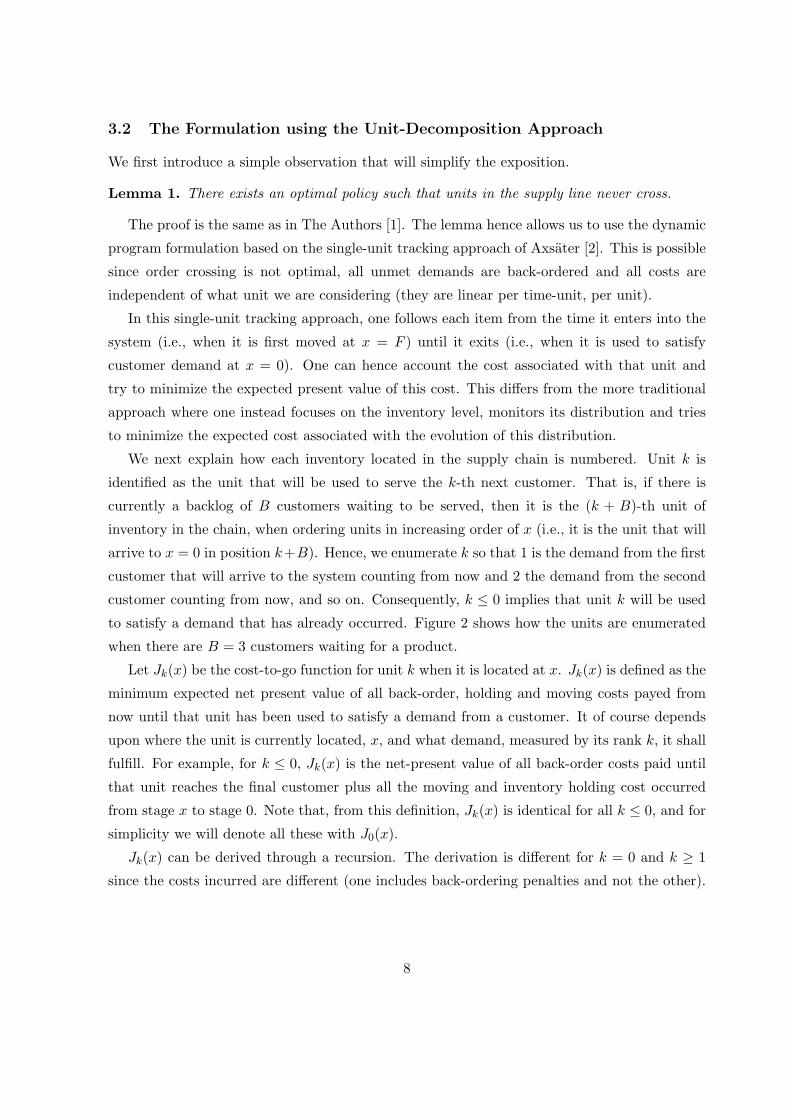
3.2 The Formulation using the Unit-Decomposition Approach

We first introduce a simple observation that will simplify the exposition.

Lemma 1. There exists an optimal policy such that units in the supply line never cross.

The proof is the same as in The Authors [1]. The lemma hence allows us to use the dynamic

program formulation based on the single-unit tracking approach of Axsater [2]. This is possible

since order crossing is not optimal, all unmet demands are back-ordered and all costs are

independent of what unit we are considering (they are linear per time-unit, per unit).

In this single-unit tracking approach, one follows each item from the time it enters into the

system (i.e., when it is first moved at x = F ) until it exits (i.e., when it is used to satisfy

customer demand at x = 0). One can hence account the cost associated with that unit and

try to minimize the expected present value of this cost. This differs from the more traditional

approach where one instead focuses on the inventory level, monitors its distribution and tries

to minimize the expected cost associated with the evolution of this distribution.

We next explain how each inventory located in the supply chain is numbered. Unit k is

identified as the unit that will be used to serve the k-th next customer. That is, if there is

currently a backlog of B customers waiting to be served, then it is the (k + B)-th unit of

inventory in the chain, when ordering units in increasing order of x (i.e., it is the unit that will

arrive to x = 0 in position k+B). Hence, we enumerate k so that 1 is the demand from the first

customer that will arrive to the system counting from now and 2 the demand from the second

customer counting from now, and so on. Consequently, k ≤ 0 implies that unit k will be used

to satisfy a demand that has already occurred. Figure 2 shows how the units are enumerated

when there are B = 3 customers waiting for a product.

Let Jk(x) be the cost-to-go function for unit k when it is located at x. Jk(x) is defined as the

minimum expected net present value of all back-order, holding and moving costs payed from

now until that unit has been used to satisfy a demand from a customer. It of course depends

upon where the unit is currently located, x, and what demand, measured by its rank k, it shall

fulfill. For example, for k ≤ 0, Jk(x) is the net-present value of all back-order costs paid until

that unit reaches the final customer plus all the moving and inventory holding cost occurred

from stage x to stage 0. Note that, from this definition, Jk(x) is identical for all k ≤ 0, and for

simplicity we will denote all these with J0(x).

Jk(x) can be derived through a recursion. The derivation is different for k = 0 and k ≥ 1

since the costs incurred are different (one includes back-ordering penalties and not the other).

8

Figure 2: An example of a continuous supply chain, from The Authors [1]. The x-axis represents the

distance of each inventory unit from the customer. Each circle represents a unit of inventory. The number

associated with its unit can be zero or negative if the unit will serve a customer that has already arrived

(there are B = 3 of them), or positive in which case it denotes the rank of the (future) customer to whom

it will go.

For k = 0,

J0(x) =

0 if x = 0

minv∈[vmin(x),vmax(x)]

{(b+ h(x) +m(x, v)

)∆+ J0(x− v∆)e−r∆

}otherwise

(1)

where ∆ is a short time interval.

If the demand has not occurred, i.e., k ≥ 1, then the future costs depend upon when the

customer arrives to the system and where the unit is at that moment. Since the demand is

generated from a Poisson process, the time until the customer arrives is Erlang distributed

with rate λ and index k, see e.g. Axsater [2]. We do not need to use this fact; we only need to

know that in a short time interval ∆, the probability of one customer arriving to the system

is λ∆ and the probability of more customer arrivals is negligible. If a customer arrives, then

the cost-to-go to be considered is the one corresponding to the (k− 1)-th unit, rather than the

k-th unit. The cost-to-go function can thus be expressed as

Jk(x) = minv∈[vmin(x),vmax(x)]

{(h(x) +m(x, v)

)∆+

((1− λ∆)Jk(x− v∆) + λ∆Jk−1(x− v∆)

)e−r∆

}(2)

Note that the derivation of Equations (1)-(2) is presented with a discrete formulation, with

time increments of ∆. In reality, in a truly continuous-stage system, Jk(x) satisfies a differential

equation, called the Hamilton-Jacobi-Bellman (HJB) equation. The technical details from the

9

continuous system are taken from optimal control theory, see Bertsekas [6]. The HJB equations

can be written as

0 = minv∈[vmin(x),vmax(x)]

(m(x, v)− v

dJ0dx

)+ b+ h(x)− rJ0(x) (3)

and for k ≥ 1,

0 = minv∈[vmin(x),vmax(x)]

(m(x, v)− v

dJkdx

)+ h(x) + λJk−1(x)− (λ+ r)Jk(x) (4)

Equations (3) and (4) are the counterparts of Equations (1)-(2) for the continuous-stage chain.

For completeness, we have the terminal conditions J0(0) = 0 and Jk(0) =

[1−

(λ

λ+ r

)k]h(0)

r.

They correspond to the expected discounted holding cost during a Erlang-distributed time with

rate λ and index k. Together, the equations above can provide a powerful scheme to obtain the

optimal policy in many settings, as shown in the next section.

4 General Solution Procedure

In this section we will derive simple closed-form solutions for the optimal policy under various

specific cost structures and provide a general procedure to find the solution under a general

cost structure. Denote v∗k(x) the optimal control for unit k at location x.

4.1 Concave Moving Costs

When m(x, v) is concave in v for all x, then Equations (3) and (4) imply that it is optimal to

set v∗k(x) = vmin(x) or vmax(x). An item will be moved at minimum speed when

m(x, vmax(x)

)−m

(x, vmin(x)

)≥

(vmax(x)− vmin(x)

)dJkdx

and at maximum speed otherwise. When vmin(x) = 0 and vmax(x) = 1, then this problem is

equivalent to the multi-echelon inventory management problem analyzed in The Authors [1],

which results, for constant and linear cost structures, in setting v∗k(x) = 1 if and only if x falls

within an interval [xLk , xHk ].

Of course, in this case there is no expediting occurring in the chain: the manager either

ships the item (selects the maximum speed), or not (selects the minimum speed). Interestingly,

this decision is the same as the one taken with linear cost

m(x, v) = m(x, vmin(x)

)+

(m(x, vmax(x)

)−m

(x, vmin(x)

))(v − vmin(x)

vmax(x)− vmin(x)

).

10

Hence, one can “convexify” the moving cost function appropriately without affecting the

optimal costs or decisions. As a result, it is sufficient to consider the case where m(x, v) is

convex in v for all x, which we do next.

4.2 Moving Costs with Normal and Express Speeds

In order to start building some intuition for convex moving costs, consider constant inventory

holding costs h(x) = h, and the following moving cost function

m(v, x) =

cnv for v ≤ vn

cnvn + ce(v − vn) for vn ≤ v ≤ ve

∞ for v > ve

where 0 < cn < ce. vn represents the “normal” speed, while ve represents a higher, “express”

speed. The resulting costs ce > cn imply that it is more expensive to move an item faster for

a given distance (the cost per time unit is more expensive, the time it takes is shorter, but

the net effect is that the total cost is higher). This results in a convex moving cost function.

Equations (3) and (4) imply that

v∗k(x) =

0 when

dJkdx

≤ cn

vn when cn ≤ dJkdx

≤ ce

ve whendJkdx

≥ ce

(5)

Let

JN0 (x) :=

b+ h(x)

rand for k ≥ 1, JN

k (x) :=h(x) + λJk−1(x)

r + λ(6)

Combining Equation (5) with (3) yields that

J0(x) = JN0 (x) when

dJ0dx

≤ cn

dJ0dx

= cn +2r(JN0 (x)− J0(x)

)vn

when 0 ≤ 2r(JN0 (x)− J0(x)

)≤ vn(ce − cn)

dJ0dx

= ce +2r(JN0 (x)− J0(x)

)− (ce − cn)vn

vewhen 2r

(JN0 (x)− J0(x)

)≥ vn(ce − cn)

(7)

11

Similarly, combining Equation (5) with (4) for k ≥ 1 yields that

Jk(x) = JNk (x) when

dJkdx

≤ cn

dJkdx

= cn +2(λ+ r)

(JNk (x)− Jk(x)

)vn

when 0 ≤ 2(λ+ r)(JNk (x)− Jk(x)

)≤ vn(ce − cn)

dJkdx

= ce +2(λ+ r)

(JNk (x)− Jk(x)

)− (ce − cn)vn

vewhen 2(λ+ r)

(JNk (x)− Jk(x)

)≥ vn(ce − cn)

(8)

Although these equations seem difficult to solve, they possess a well-behaved structure. One

can characterize this structure, as done in the next theorem.

Theorem 1. Normal and express moving costs and fixed holding costs. For k ≥ 0,

there exists xL,nk ≤ xL,ek ≤ xH,ek ≤ xH,n

k such that

• v∗k(x) = 0 for x ≤ xL,nk or x ≥ xH,nk ;

• v∗k(x) = vn for xL,nk ≤ x ≤ xL,ek or xH,ek ≤ x ≤ xH,n

k ;

• v∗k(x) = ve for xL,ek ≤ x ≤ xH,ek .

In addition the sequences xL,nk and xL,ek are non-decreasing in k, while xH,ek and xH,n

k are non-

increasing in k.

The theorem hence shows that the optimal speed is first increasing and then decreasing in

x. Interestingly, this result generalizes to multiple speed levels the order/no-order policy of

The Authors [1]. Figure 3 illustrates the result. In particular, the figure shows that one should

only expedite for low k and x neither too close nor too far from the customer. One can also

interpret the curves as follows: it is optimal to expedite unit k down to xL,ek if xL,ek ≤ x ≤ xH,ek ;

otherwise, it is optimal to move unit k at normal speed down to xL,nk if xL,nk ≤ x ≤ xH,nk .

Alternatively, at a given stage x, one should request expedited delivery up to the dashed line,

and normal delivery up to the solid line.

4.3 Quadratic Moving Costs

The moving cost was piecewise-linear and convex in the previous section. This resulted in

regions where the optimal speed was fixed, which allowed us to prove the structure of the

optimal expediting policy. We focus now on the quadratic cost case, where m(x, v) =1

2v2,

vmin(x) = 0 and vmax(x) = ∞. Interestingly, World Economic Forum [21] (p.17) observed

that maritime transportation costs, as depicted in Figure 1, can be approximated well by a

quadratic function of speed.

12

0 1 2 3 4 5 6 7 8 9 10

0

1

2

3

4

5

6

7

8

9

10

11

12

13

14

Stage x

k

Express deliveryNormal delivery

CHOOSE vk*(x)=vn

CHOOSE vk*(x)=ve

Ship normally item k=10 if 4.04 ≤ x

Expedite item k=1 if 0.31 ≤ x ≤ 5.85

Figure 3: Illustration of the optimal policy with vn = 0.5, ve = 1, and costs cn = 4, ce = 10, with

b = 10, h = 1, r = 10%, λ = 1. The solid line delimits from above the region where v∗k(x) = vn, while the

dashed line delimits the regions where v∗k(x) = vn (above) and v∗k(x) = ve (below).

In this case, Equations (3) and (4) imply that

v∗k(x) = max

{0,

dJkdx

}. (9)

In contrast with the previous section, one cannot rely on the fact that the optimal speed is

piece-wise constant anymore. Now, the HJB equations can be written as

dJ0dx

=

√2r(JN0 (x)− J0(x)

)(10)

and for k ≥ 1,dJkdx

=

√2(λ+ r)

(JNk (x)− Jk(x)

)(11)

These equations are non-standard differential equations. Interestingly, it can be seen that

v∗k(x) = 0 if and only if Jk(x) = JNk (x). Otherwise, Jk(x) < JN

k (x). From the Picard-Lindelof

theorem, if JNk (x) − Jk(x) > 0, then the square-root function is locally Lipschitz-continuous

and as a result, there is a unique solution to the differential equation.

13

Let the inventory cost be constant again, h(x) = h. Consider the decision for k = 0. It turns

out that the solution can be provided in closed-form. For this purpose, let xH =

√2(b+ h)

r2,

and we have

J0(x) =b+ h

r− r

2

(max{0, xH − x}

)2.

Note that xH is such that J0(0) = 0. We can again find some general properties of Jk(x).

Theorem 2. Quadratic transportation costs and fixed holding costs. For k ≥ 0,

v∗k =dJkdx

is first increasing and then decreasing, i.e., it is quasi-concave.

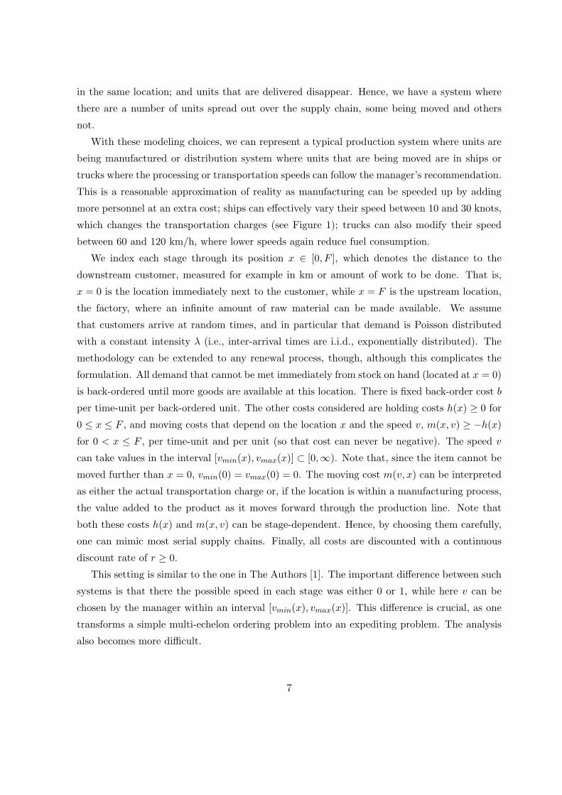
This result provides an interesting insight the optimal speeds to be chosen for each unit.

Indeed, Equation (9) implies that the optimal speed is first increasing in x and then decreasing.

Hence, when a unit is very close to the customer, it is being slowed down, while a unit that

is being very far from the customer, it is being accelerated. This extends the insight from

Theorem 1 to quadratic speeds. Also, in the proof of the theorem one can directly show that

for all x, k ≥ 0, 0 ≤ v∗k+1(x) ≤ v∗k(x), which provides in this scenario a different proof of Lemma

1.

Figure 4 illustrates Theorem 2 for a cost function equal to 5v2 relative to a holding cost of

h = 1 and a back-ordering penalty of b = 10. As a result, for k = 0 one should set a speed

equal to√2.2 ≈ 1.48 close to x = 0 (which is the maximum across all x, k), while for k = 10,

the speed is close to 0 around x = 0.

4.4 General Convex Moving Costs

After observing how Theorems 1 and 2 rely on the same problem structure, one may wonder

whether it is generally true that v∗k is quasi-concave. We establish below general sufficient

conditions for this to be true.

We consider here that h(x) may be non-constant, and assume that m(x, v) is convex in v

for all x. We also assume thatdm

dv(vmin(x), x) = 0 and

dm

dv(vmax(x), x) = ∞, which implies

that the marginal transportation cost increases from zero, at the minimum acceptable speed,

to infinity, at the maximum one. For each x, define s(x, c) the lowest s such thatdm

dv(s, x) = c,

which is well-defined for all c ≥ 0 (in fact there may be several s in a given interval that

satisfy the equation, we set it to be the lowest). Clearly, since m is convex, s is increasing in c.

Equations (3) and (4) imply that

v∗k(x) = s

(x,

dJkdx

)(12)

14

0 2 4 6 8 100

2

4

6

8

10

12

14

Stage x

k

Optimal speeds vk*(x)

0

0.2

0.4

0.6

0.8

1

1.2

Figure 4: Illustration of the optimal policy with m(x, v) = 5v2, with b = 10, h = 1, r = 10%, λ = 1. The

level sets shown at the right hand side represent the levels of the optimal speeds chosen at each x, k. The

lighter the color, the faster an item should be shipped.

In addition, let

K (x, c) = − minv∈[vmin(x),vmax(x)]

(m(x, v)− vc) = −m(x, s(x, c)

)+ s(x, c)c ≥ 0.

Note that∂K

∂c= s(x, c) and hence K is convex increasing in c. As a result, for a given x, one

can define ϕ(x,C) as the unique value such that K (x, ϕ(x,C)) = C. ϕ is concave increasing in

C for each x. Equations (3) and (4) can be rewritten as

dJ0dx

= ϕ(x, r

(JN0 (x)− J0(x)

))≥ 0 (13)

and for k ≥ 1,dJkdx

= ϕ(x, (λ+ r)

(JNk (x)− Jk(x)

))≥ 0. (14)

If ϕ possesses some properties, we can show that the optimal speed v∗k is first increasing and

then decreasing. The following theorem identifies these properties.

15

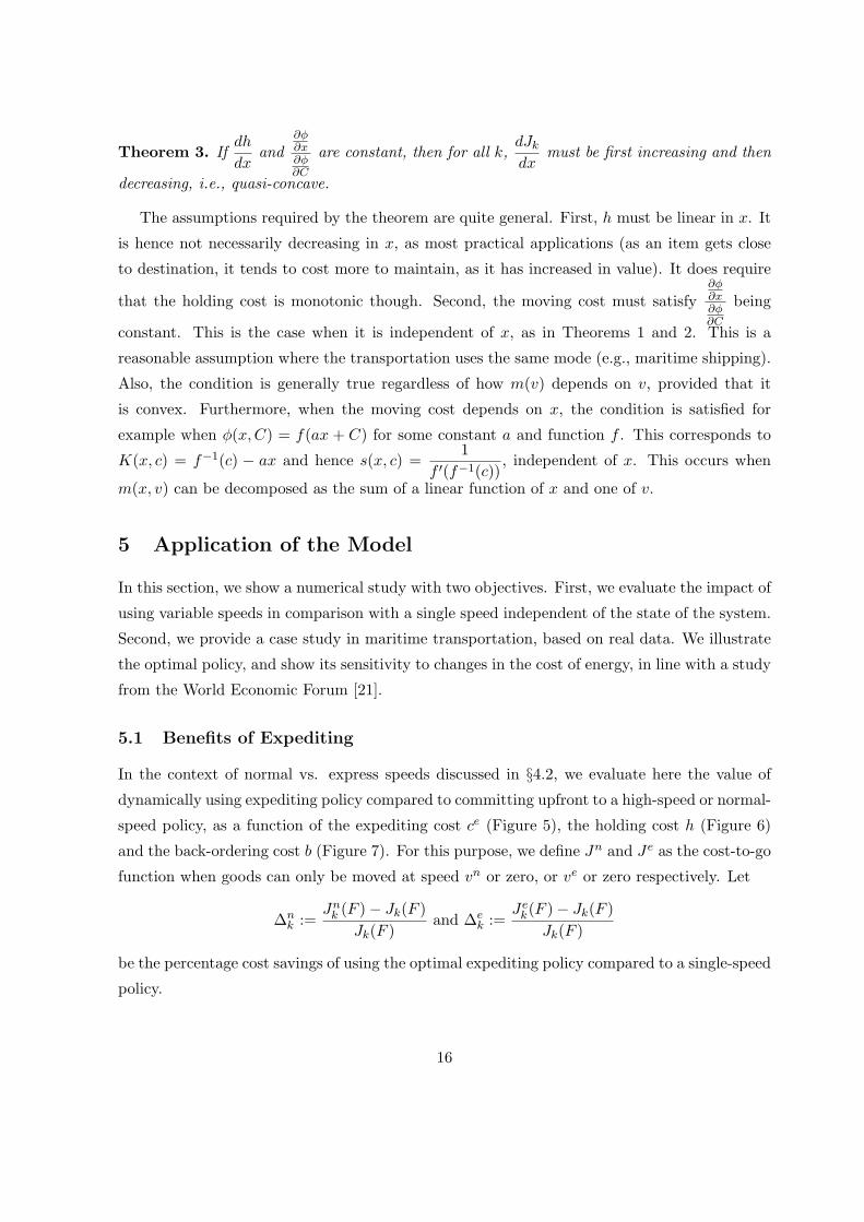
Theorem 3. Ifdh

dxand

∂ϕ∂x∂ϕ∂C

are constant, then for all k,dJkdx

must be first increasing and then

decreasing, i.e., quasi-concave.

The assumptions required by the theorem are quite general. First, h must be linear in x. It

is hence not necessarily decreasing in x, as most practical applications (as an item gets close

to destination, it tends to cost more to maintain, as it has increased in value). It does require

that the holding cost is monotonic though. Second, the moving cost must satisfy∂ϕ∂x∂ϕ∂C

being

constant. This is the case when it is independent of x, as in Theorems 1 and 2. This is a

reasonable assumption where the transportation uses the same mode (e.g., maritime shipping).

Also, the condition is generally true regardless of how m(v) depends on v, provided that it

is convex. Furthermore, when the moving cost depends on x, the condition is satisfied for

example when ϕ(x,C) = f(ax + C) for some constant a and function f . This corresponds to

K(x, c) = f−1(c) − ax and hence s(x, c) =1

f ′(f−1(c)), independent of x. This occurs when

m(x, v) can be decomposed as the sum of a linear function of x and one of v.

5 Application of the Model

In this section, we show a numerical study with two objectives. First, we evaluate the impact of

using variable speeds in comparison with a single speed independent of the state of the system.

Second, we provide a case study in maritime transportation, based on real data. We illustrate

the optimal policy, and show its sensitivity to changes in the cost of energy, in line with a study

from the World Economic Forum [21].

5.1 Benefits of Expediting

In the context of normal vs. express speeds discussed in §4.2, we evaluate here the value of

dynamically using expediting policy compared to committing upfront to a high-speed or normal-

speed policy, as a function of the expediting cost ce (Figure 5), the holding cost h (Figure 6)

and the back-ordering cost b (Figure 7). For this purpose, we define Jn and Je as the cost-to-go

function when goods can only be moved at speed vn or zero, or ve or zero respectively. Let

∆nk :=

Jnk (F )− Jk(F )

Jk(F )and ∆e

k :=Jek(F )− Jk(F )

Jk(F )

be the percentage cost savings of using the optimal expediting policy compared to a single-speed

policy.

16

We set h(x) = h for 0 ≤ x < F , and h(F ) = 0. This implies that the firm does not pay

any holding cost for an item that has not been ordered or initiated in production. From a

practical perspective, this is reasonable because the first step in the process typically entails

a procurement decision, and holding costs are not paid until the units enter the system. In

addition, this assumption will help us compare the cost savings fairly. Indeed, for a high value

of k, all of the policies (single or variable speeds) will decide not to move item k. As a result,

from Equation (6), we know that Jk(F ) = JNk (F ) =

λ

r + λJk−1(F ) and similarly for Jn

k (F )

and Jek(F ). This implies that ∆n

k = ∆nk−1 and ∆e

k = ∆ek−1. As a result, we can use ∆n

∞,∆e∞

as an indicator of the potential savings of expediting. This would not be true if h(F ) = 0, as

∆nk ,∆

ek → 0 as k goes to infinity.

Note also that the assumption might invalidate the use of Theorem 1 at x = F . Indeed,

Jk, Jnk and Je

k are well-defined for x < F and Theorem 1 can be applied. However, Jk may

become discontinuous at x = F . To resolve this potential issue, one must define Jk(F ) as the

minimum of the solution of the HJB-equation, i.e., limx→F Jk(x), and JNk (F ) =

λ

r + λJk−1(F ).

The same is true for Jnk (F ) and Je

k(F ). For further details on this type of discontinuity, see

The Authors [1].

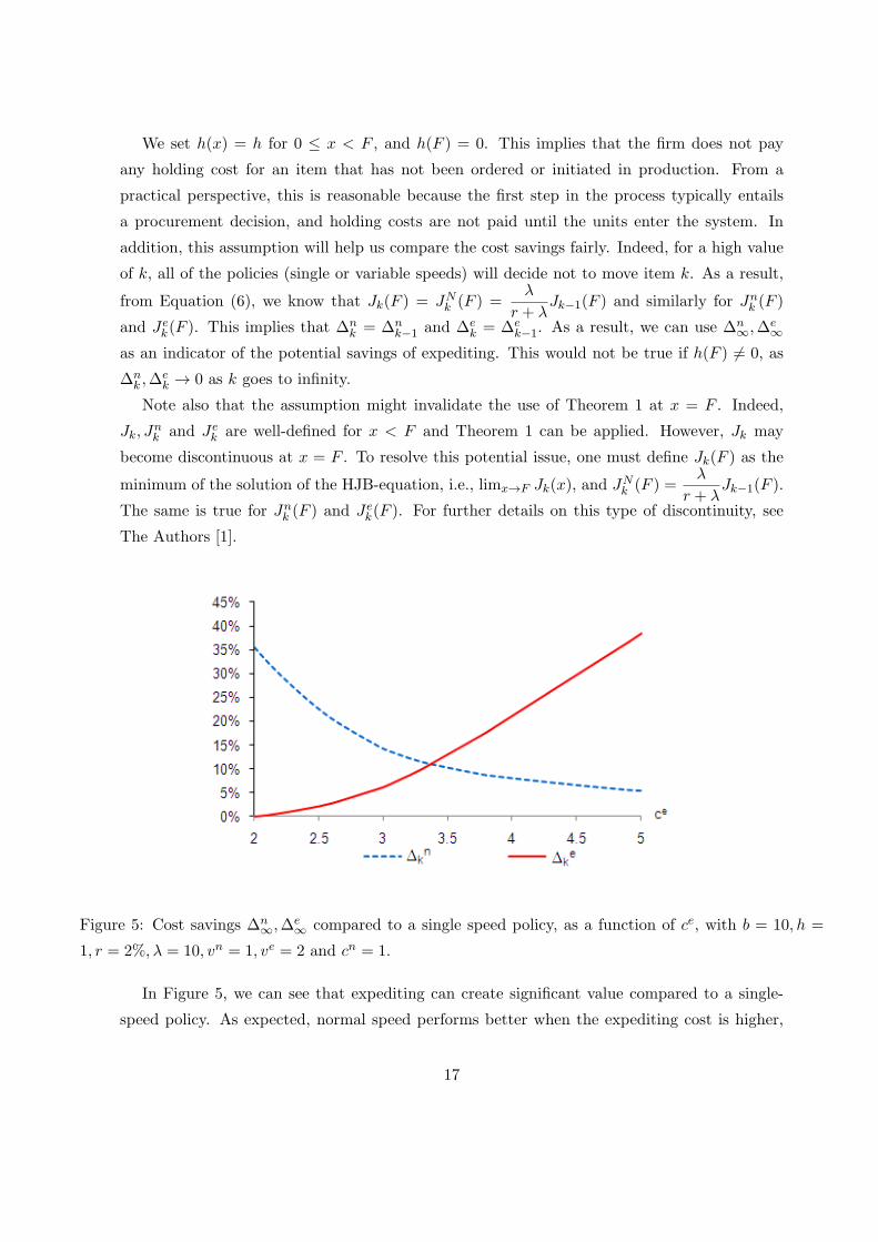
Figure 5: Cost savings ∆n∞,∆e

∞ compared to a single speed policy, as a function of ce, with b = 10, h =

1, r = 2%, λ = 10, vn = 1, ve = 2 and cn = 1.

In Figure 5, we can see that expediting can create significant value compared to a single-

speed policy. As expected, normal speed performs better when the expediting cost is higher,

17

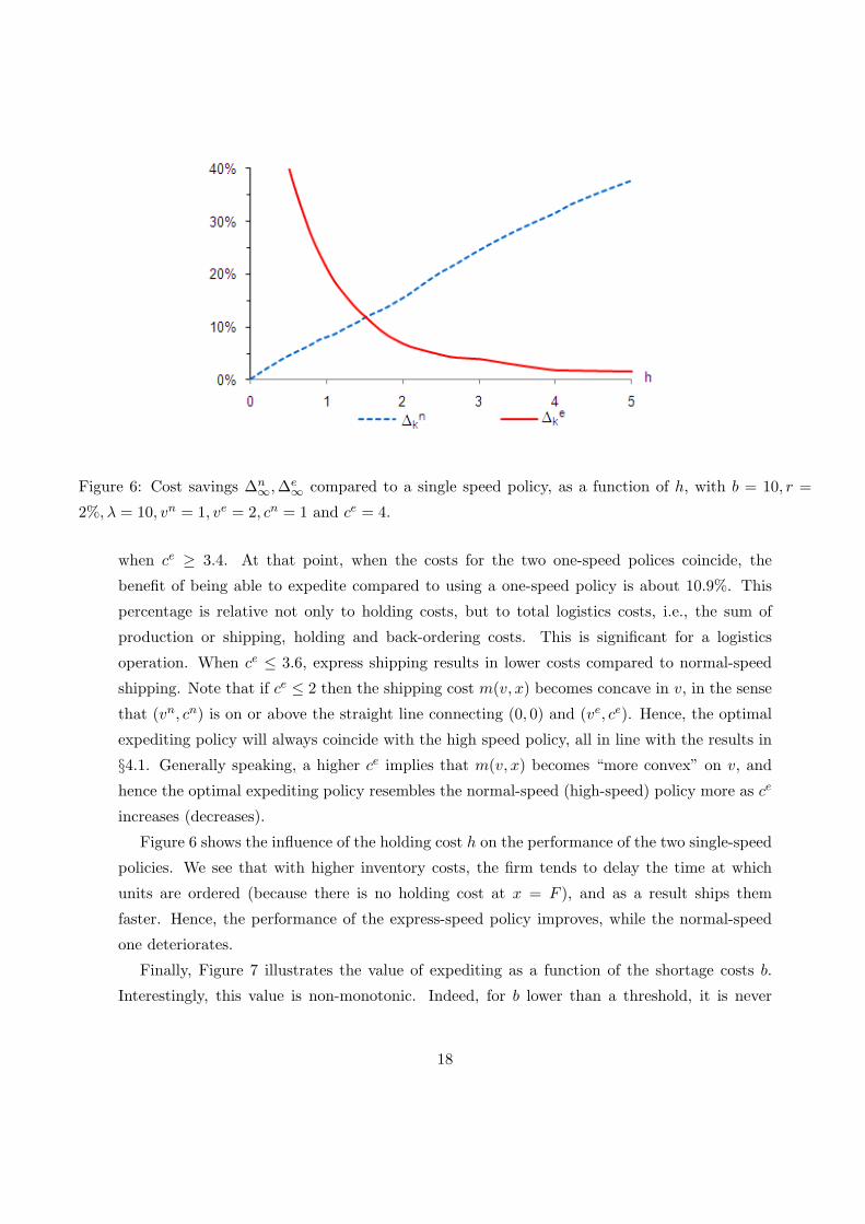
Figure 6: Cost savings ∆n∞,∆e

∞ compared to a single speed policy, as a function of h, with b = 10, r =

2%, λ = 10, vn = 1, ve = 2, cn = 1 and ce = 4.

when ce ≥ 3.4. At that point, when the costs for the two one-speed polices coincide, the

benefit of being able to expedite compared to using a one-speed policy is about 10.9%. This

percentage is relative not only to holding costs, but to total logistics costs, i.e., the sum of

production or shipping, holding and back-ordering costs. This is significant for a logistics

operation. When ce ≤ 3.6, express shipping results in lower costs compared to normal-speed

shipping. Note that if ce ≤ 2 then the shipping cost m(v, x) becomes concave in v, in the sense

that (vn, cn) is on or above the straight line connecting (0, 0) and (ve, ce). Hence, the optimal

expediting policy will always coincide with the high speed policy, all in line with the results in

§4.1. Generally speaking, a higher ce implies that m(v, x) becomes “more convex” on v, and

hence the optimal expediting policy resembles the normal-speed (high-speed) policy more as ce

increases (decreases).

Figure 6 shows the influence of the holding cost h on the performance of the two single-speed

policies. We see that with higher inventory costs, the firm tends to delay the time at which

units are ordered (because there is no holding cost at x = F ), and as a result ships them

faster. Hence, the performance of the express-speed policy improves, while the normal-speed

one deteriorates.

Finally, Figure 7 illustrates the value of expediting as a function of the shortage costs b.

Interestingly, this value is non-monotonic. Indeed, for b lower than a threshold, it is never

18

Figure 7: Cost savings ∆n∞,∆e

∞ compared to a single speed policy, as a function of b, with h = 1, r =

2%, λ = 10, vn = 1, ve = 2, cn = 1 and ce = 4.

optimal to use express speed. As a result, ∆n∞ = 0. However, ∆e

∞ is decreasing. This is

true because the average back-ordering time is typically lower with express speeds compared

to normal speeds (the discrete choice of highest k that is released into the system may cause

the time difference to jump up or down, though). Hence as b increases in this range, the

cost of the express-speed policy increases slower than the normal-speed one. In contrast, for b

above the threshold, the benefit of being able to adjust the speed to the demand is increasing

in the shortage cost b, no matter which single-speed policy one considers. Intuitively, this

is not surprising because the higher the back-ordering cost is, the more valuable it is to be

able reduce the waiting time of a customer through expediting. Upon closer observation, one

can see that, independently of which policy is used, the base-stock level at which a unit is

released into the system is non-decreasing with b. This is true because it becomes beneficial

to pay additional holding costs to avoid paying more expensive back-orders. Hence, there

are more units in transit, and each unit is in transit for a longer period of time. Given that

the number of uncertain events that occur during this period becomes higher (the amount of

demand uncertainty is larger), there is greater value of being able to adjust the decisions, i.e.,

speeding up a unit when needed, or using the more economical normal speed if the demand is

low.

19

5.2 A Case Study

In a recent study, the World Economic Forum [21] suggested that “despeeding the supply

chain” is among the most valuable levers to reduce future CO2 emissions. They considered

reducing the speed of road vehicles (e.g., from 65 to 62 mph in the USA) and ships (with

quadratic shipping cost as a function of speed). In their study, they found that “the single

biggest opportunity within this calculation is to reduce the speed at which ships travel as a

result of the squared relationship between speed and emissions”. However, it is not clear what

impact the speed reduction would have on inventory, which is also a driver of supply chain cost.

In this section, we provide a case study with a similar objective: we want to evaluate the

potential for cost reduction of modulating ocean transportation speed to the state of the system.

Similarly to World Economic Forum [21], we also consider a quadratic shipping cost function,

given by the data from Figure 1. We calculate the optimal policy for several scenarios of fuel

cost, which would factor in the cost of new CO2 emission rights or taxes.

The benchmark that we use corresponds to the export of paper and derived products from

Sweden to China. This is one of the biggest export products both in tonnage and value. Ac-

cording to data from Statistics Sweden (www.scb.se), this export amounted to 302,910 metric

tons and a value of over 2 billion Swedish crowns (SEK) in 2009. This yearly demand corre-

sponds to the capacity of about six S-class vessels per year, i.e., λ = 0.017 ship loads per day.

The average value of a ship-load is 350 million SEK. Using an exchange rate of around 7.5

SEK/USD and an interest rate of r = 10% p.a. provides a holding cost h(x) = 12, 000 USD per

ship load per day, for 0 ≤ x < F . As before, we assume that no holding cost is paid until the

transportation is initiated, i.e., h(F ) = 0. The shortage cost is set to be 10 times the holding

cost, i.e., b = 120, 000 USD per ship load per day.

The moving cost can be estimated using two elements: first, we need to account for the rent

of the ship; second, we need to include the fuel cost. The Baltic Dry index gives the spot prices

for the daily rent for ships of various types. An estimate of the total cost for operating a ship

can be obtained by using the average of the Baltic Dry index over 2009 which has been around

20,000 USD per day. The fuel consumption is given by Figure 1 and the moving cost will be

obtained by multiplying this with f , the cost of fuel in USD/ton and adding the rental charge.

The resulting moving cost is m(x, v) = 20, 000 + f ·(0.71v2 − 6.17v

)USD per day given that

the velocity is measured in knots, for 0 < x ≤ F . Note that m(0, 0) = 0. To ensure a realistic

use of the data, we limit the possible speeds to be in the range [10,30] knots. Furthermore, the

distance between Sweden and China through the Suez Canal is about 11,000 nautical miles,

i.e., F = 11, 000.

20

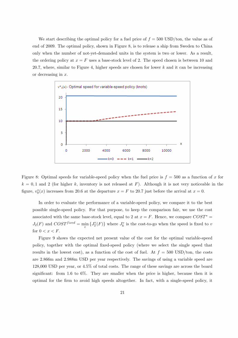
We start describing the optimal policy for a fuel price of f = 500 USD/ton, the value as of

end of 2009. The optimal policy, shown in Figure 8, is to release a ship from Sweden to China

only when the number of not-yet-demanded units in the system is two or lower. As a result,

the ordering policy at x = F uses a base-stock level of 2. The speed chosen is between 10 and

20.7, where, similar to Figure 4, higher speeds are chosen for lower k and it can be increasing

or decreasing in x.

Figure 8: Optimal speeds for variable-speed policy when the fuel price is f = 500 as a function of x for

k = 0, 1 and 2 (for higher k, inventory is not released at F ). Although it is not very noticeable in the

figure, v∗0(x) increases from 20.6 at the departure x = F to 20.7 just before the arrival at x = 0.

In order to evaluate the performance of a variable-speed policy, we compare it to the best

possible single-speed policy. For that purpose, to keep the comparison fair, we use the cost

associated with the same base-stock level, equal to 2 at x = F . Hence, we compare COST ∗ =

J2(F ) and COST fixed = minv

{Jv2 (F )} where Jv

k is the cost-to-go when the speed is fixed to v

for 0 < x < F .

Figure 9 shows the expected net present value of the cost for the optimal variable-speed

policy, together with the optimal fixed-speed policy (where we select the single speed that

results in the lowest cost), as a function of the cost of fuel. At f = 500 USD/ton, the costs

are 2.866m and 2.988m USD per year respectively. The savings of using a variable speed are

128,000 USD per year, or 4.5% of total costs. The range of these savings are across the board

significant: from 1.6 to 6%. They are smaller when the price is higher, because then it is

optimal for the firm to avoid high speeds altogether. In fact, with a single-speed policy, it

21

Figure 9: In the top figure, cost of the optimal expediting policy with variable speed and the optimal policy

with a fixed speed. In the bottom one, the optimal speed for the fixed speed policy. The curves are shown

as functions of the fuel cost, f .

22

becomes optimal to use the most fuel-economic speed of 10 knots.

Furthermore, we are also interested in evaluating how much CO2 can be saved by using

variable speeds. Figure 10 illustrates the average amount of fuel consumed per voyage as a

function of the fuel price. The fuel consumption is non-increasing in the fuel price. This is

indeed true as the firm is more inclined to decrease the speed and the fuel consumption when the

savings in transportation cost are larger even if this comes at the expense of increased holding

cost. Notice also that there are large jumps down in the fuel consumption. These coincide with

an increased optimal base-stock level at F , i.e., a permanent increase in the number of ships on

route to China. Each ship has thus a longer time to get to the destination before the demand

is realized so it can use a slower and more fuel-efficient speed. These shifts in base-stock level

occur at different fuel prices for the different policies (variable- and single-speed) so no policy

dominates the other with respect to CO2 emissions over the entire interval. However, the figure

clearly identifies that it is possible to significantly reduce CO2 emissions by increasing the price

of fuel above the level where more ships are used. In other words, the recommendation of World

Economic Forum [21] can actually be implemented through a well-designed taxing mechanism,

that involves an increase on the amount of ships and inventory in the supply chain.

Figure 10: Fuel consumed in the optimal expediting policy and the optimal policy with a fixed speed.

6 Conclusion and Further Research

This paper analyzes the optimal expediting decisions of a firm that needs to move an item

from an initial location into the market, where customers arrive following a Poisson process.

23

This can be interpreted as a transportation problem, where the speed of shipping must be

determined, or a production problem, where the amount of work to be done onto the item per

time period can be increased or decreased over time. Using a continuous formulation of the

problem and the observation that the problem can be decomposed unit by unit, we identify

the optimal control policy through the solution of a differential equation, the HJB equation.

The approach is conceptually simple and through a proper setting of parameters (the holding

and moving cost as a function of the location, x and speed v) can mimic many practical

problems. Under certain regularity conditions on the cost parameters, the approach yields new

insights regarding the optimal speed at which items are moved: for any item, associated with a

particular customer demand, the optimal speed is first increasing in the distance to the market,

and then decreasing. In addition to theoretical results, we also provide a numerical study

where we demonstrate that using expediting through variable speeds can provide substantial

savings. For example, in a Europe-Asia shipping problem, we estimate the savings at 4.5%

of total logistics cost (transportation, inventory holding and back-ordering), using 2009 data.

This study hence illustrates the potential of our solution method for improving cost efficiency

and for supporting policy-making decisions such as emissions control.

This work has a number of possible extensions. The methodology used in the paper can be

directly applied to other demand specifications as long as they follow a renewal process, e.g.,

compound Poisson. It can also be used in situations where demand occurs unit by unit but

orders are placed in batches of a fixed size. Moreover, uncertainty in the cost parameters should

also fit within the general framework because it guarantees no orders crossings. Furthermore, an

interesting line of future research is to explore how the methodology can be altered to account

for possible order-crossings. Consider for example a modification of our model that includes a

fixed cost associated with changing the speed and/or when this can only be done at a limited

number of locations. In this setting, units might cross as it can be optimal to set a high speed

for one unit even if there are others moving at a slower speed in front of it. It is certainly

analytically challenging to adapt the solution approach to this situation, but at the same time

this would shed new light on the problem.

24

References

[1] The Authors 2011. “A Characterization of Optimal Base-Stock Levels for a Continuous-

Stage Serial Supply Chain.” Working paper.

[2] Axsater S. 1990. “Simple Solution Procedure for a Class of Two-Echelon Inventory Prob-

lems.” Operations Research, 38(1), pp. 64-69.

[3] Axsater S. and P. Lundell 1984. “In-Process Safety Stocks.” Proceedings of the 23rd

Conference on Decision and Control in Las Vegas NV 1984.

[4] Axsater S. and K. Rosling 1993. “Installation vs. Echelon Stock Policies for Multilevel

Inventory Control.” Management Science, 39(10), pp. 1274-1280.

[5] Berling P. and V. Martınez-de-Albeniz 2009. “Optimal Inventory Policies when Purchase

Price and Demand are Stochastic.” Forthcoming in Operations Research.

[6] Bertsekas D. P. 2000. Dynamic Programming and Optimal Control. Athena Scientific,

Belmont, Massachusetts.

[7] Chen F. and Y. S. Zheng. 1994. “Lower Bounds for Multi-Echelon Stochastic Inventory

Systems.” Management Science, 40(11), pp. 1426-1443.

[8] Clark A. J. and H. Scarf 1960. “Optimal Policies for a Multi-Echelon Inventory Problem.”

Management Science, 6(4), pp. 475-490.

[9] Federgruen A. and P. Zipkin 1984. “Computational Issues in an Infinite-Horizon, Multi-

echelon Inventory Model.” Operations Research, 32(4), pp. 818-836.

[10] Gallego G., Y. Jin, A. Muriel, G. Zhang and V. T. Yildiz 2007. “Optimal Ordering Policies

with Convertible Lead Times.” European Journal of Operations Research, 176(2), pp.

892-910.

[11] Janakiraman G. and J. A. Muckstadt 2009. “A Decomposition Approach for a Class of

Capacitated Serial Systems.” Operations Research, 57(6), pp. 1384-1393.

[12] Jain A., H. Groenevelt and N. Rudi 2010. “Continuous Review Inventory Model with

Dynamic Choice of Two Freight Modes with Fixed Costs.” Manufacturing and Service

Operations Management, 12(1), pp. 120-139.

[13] Kim C., D. Klabjan and D. Simchi-Levi 2006. “Optimal Policy for a Periodic Review

Inventory System with Expediting.” Working paper, MIT.

[14] Lawson D. G. and E. L. Porteus 2000. “Multistage Inventory Management with Expedit-

ing.” Operations Research, 48(6), pp. 878-893.

25

[15] Martınez-de-Albeniz V. and A. Lago 2010. “Myopic Inventory Policies Using Individ-

ual Customer Arrival Information.” Manufacturing and Service Operations Management,

12(4), pp. 663-672.

[16] Minner S. 2003. “Multiple-supplier inventory models in supply chain management: A

review.” Int. J. Production Econom. 81 - 82, pp. 265279.

[17] Moinzadeh K. and C. P. Schmidt. 1991. “An (S - 1, S) Inventory System with Emergency

Orders.” Operations Research 39(2), pp. 308321.

[18] Muharremoglu A. and J. N. Tsitsiklis 2008. “A Single-Unit Decomposition Approach to

Multiechelon Inventory Systems.” Operations Research, 56(5), pp. 1089-1103.

[19] Muharremoglu A. and J. N. Tsitsiklis 2003. “Dynamic Leadtime Management in Supply

Chains.” Working paper, Graduate School of Business, Columbia University.

[20] Song J.-S. and P. H. Zipkin 2009. “Inventories with Multiple Supply Sources and Networks

of Queues with Overflow Bypasses.” Management Science, 55(3), pp. 362-372.

[21] World Economic Forum 2009. “Supply Chain Decarbonization: The Role of Logis-

tics and Transport in Reducing Supply Chain Carbon Emissions.” Technical report.

http://www.weforum.org/pdf/ip/SupplyChainDecarbonization.pdf

[22] Yu Y. and S. Benjaafar 2009. “A Customer-Item Decomposition Approach to Stochastic

Inventory Systems with Correlation.” Working paper, University of Minnesota.

26

Appendix

Proof of Lemma 1

Proof. Consider an optimal policy and one sample path where two units cross. That is, unit 1

is ordered earlier than unit 2 (the time where it is moved at x = L is strictly smaller for 1) but

unit 2 arrives to x = 0 earlier than 1 (the time where unit 2 arrives at x = 0 is strictly smaller

than for 1). Since the movement is continuous, if two units cross, consider the earliest time

where they coincide in the same stage x. Since the moving and holding costs are independent

of how stage x was reached, one can always choose to move unit 1 first, without changing the

costs incurred. Consequently, order crossing cannot strictly reduce the cost, and a non-crossing

policy is also optimal.

Proof of Theorem 1

Proof. We show by induction that, for k ≥ 0,dJkdx

is positive, first increasing and then

decreasing.

For k = 0, consider Equation (7). We see that while J0 < JN0 , J0 is increasing, and when it

reaches JN0 (which is a constant), J0 becomes constant. Differentiating (7) yields

d2J0dx2

= 0 whendJ0dx

≤ cn

d2J0dx2

=2r(dJN

0dx − dJ0

dx

)vn

≤ 0 when 0 ≤ 2r(JN0 (x)− J0(x)

)≤ vn(ce − cn)

d2J0dx2

=2r(dJN

0dx − dJ0

dx

)ve

≤ 0 when 2r(JN0 (x)− J0(x)

)≥ vn(ce − cn)

It is hence clear thatdJ0dx

is positive and decreasing, which validates the induction property

at k = 0. Hence J0 is increasing concave. This shows the existence of xL,n0 = xL,e0 = 0 and

0 ≤ xH,e0 ≤ xL,e0 .

For k ≥ 1, assume that the property is true for k−1. HencedJN

k

dxis positive, first increasing

and then decreasing. Consider Equation (8). Differentiating (8) yields

d2Jkdx2

=d2JN

k

dx2when

dJkdx

≤ cn

d2Jkdx2

=2r(dJN

kdx − dJk

dx

)vn

when 0 ≤ 2(λ+ r)(JNk (x)− Jk(x)

)≤ vn(ce − cn)

d2Jkdx2

=2r(dJN

kdx − dJk

dx

)ve

when 2(λ+ r)(JNk (x)− Jk(x)

)≥ vn(ce − cn)

27

and when at points whered2Jkdx2

= 0,

d3Jkdx3

=d3JN

k

dx3when

dJkdx

≤ cn

d3Jkdx3

=2r(d2JN

kdx2

)vn

when 0 ≤ 2(λ+ r)(JNk (x)− Jk(x)

)≤ vn(ce − cn)

d3Jkdx3

=2r(d2JN

kdx2

)ve

when 2(λ+ r)(JNk (x)− Jk(x)

)≥ vn(ce − cn)

Denote xMk−1 the maximizer ofdJk−1

dx. For x ≤ xMk−1, consider a point where

dJ2k

dx2= 0. From the

equation above,d2JN

k

dx2≥ 0, and hence

dJkdx

reaches a minimum. Since Jk(0) = JNk (0) (one can

not move the item at zero), then in the vicinity of zero, v∗k(x) = 0 andd2Jkdx2

=d2JN

k

dx2≥ 0. As a

result, for 0 ≤ x ≤ xMk−1,dJkdx

remains increasing. Let xMk := min

{x > xMk−1

∣∣∣∣d2Jkdx2= 0

}. With

the same argument as above, in this region any point such thatd2Jkdx2

= 0 satisfiesd2JN

k

dx2≤ 0,

and hencedJkdx

reaches a maximum at any such point. Since for a continuous function two

maxima must have a minimum in between, it follows that this maximum must be unique.

Hence, for x > xMk ,dJkdx

is decreasing. The existence of xL,nk ≤ xL,ek ≤ xH,ek ≤ xL,ek follows,

which completes the induction.

Finally, from Lemma 1, it must be true that xL,nk , xL,ek are non-decreasing and xH,ek , xL,ek are

non-increasing.

Proof of Theorem 2

Proof. We show by induction that, for k ≥ 1:

• there is a unique xMk ≤ xH such thatdJkdx

is non-decreasing when x ≤ xMk and non-

increasing when x ≥ xMk

• 0 ≤ dJkdx

≤ dJk−1

dx.

To initialize the induction, recall that J0 is found in closed form. xM0 := 0 is the maximum

ofdJ0dx

.

For k ≥ 1, let Dk = JNk − Jk ≥ 0, which satisfies Dk(0) = 0. From the optimality condition,

we have thatdDk

dx=

λ

r + λ

dJk−1

dx−

√2(λ+ r)Dk. (15)

28

If k = 1, we first show that the solution of this differential equation with D1(0) = 0

satisfies D1(xH) = 0 as well. Indeed, let Jmax

1 :=h

r+

b

r

(λ

λ+ r

). It turns out that D1(x) =

a

2

(max{0, xH − x}

)2satisfies the differential equation for some a > 0 such that a =

λr

r + λ−√

(λ+ r)a. Note that this implies that√

(λ+ r)a ≤ r.

For this solution, D1(0) > 0. Since the solution to the differential is unique in (0, xH), then

the solution satisfying D1(0) = 0 must stay below D1 in the entire range. As a result, since

D1 ≥ 0, it must tend to zero at xH .

Let us now prove that D1 is first increasing and then decreasing. Indeed, consider a value

xM1 wheredD1

dx(xM1 ) = 0. Differentiating Equation (15) at xM1 implies

d2Dk

dx2=

λ

r + λ

d2J0dx2

≤ 0.

Hence it is a maximum and since a continuous function cannot have two maxima without a

minimum in between, such xM1 is unique. As a result,dJ1dx

=√

2(λ+ r)D1(x) is first increasing

and then decreasing. Also, 0 ≤ dJ1dx

=√

2(λ+ r)D1(x) ≤√

(λ+ r)amax{0, xH − x} ≤

rmax{0, xH − x} =dJ0dx

.

Similarly, for k > 1, since 0 ≤ dJk−1

dx≤ dJk−2

dx, and Dk−1(0) = Dk(0) = 0, Equation (15)

implies that Dk−1 ≥ Dk ≥ 0. For x ≤ xMk−1, ifdD1

dx(x) = 0, then differentiating Equation (15)

yields thatd2Dk

dx2=

λ

r + λ

d2Jk−1

dx2≥ 0, which means that

dD1

dx(x) becomes positive afterwards.

SincedD1

dx(0) ≥ 0,

dD1

dxstays non-negative in [0, xMk−1]. On the other hand, for x ≤ xMk−1, if

dD1

dx(x) = 0, then differentiating Equation (15) yields that

d2Dk

dx2=

λ

r + λ

d2Jk−1

dx2≤ 0, which

means thatdD1

dx(x) becomes negative afterwards and stays negative until xH . Also, since Dk(x)

must decrease to zero at xH , there must exist a unique xMk ≥ xMk−1 before which Dk increases

and after which it decreases. As a result,dJkdx

=√

2(λ+ r)Dk(x) is first increasing and then

decreasing. Since Dk−1 ≥ Dk ≥ 0, 0 ≤ dJkdx

≤ dJk−1

dx. This completes the induction.

Proof of Theorem 3

Proof. First, recall that, from the definition of ϕ, we have∂ϕ

∂C=

1∂C∂c

=1

s(x, ϕ)≥ 0. Let

a :=∂ϕ∂x∂ϕ∂C

and h′ =dh

dx, constant.

We show by induction thatdJkdx

is quasi-concave.

29

For k = 0, we can differentiate Equation (13), which yields

d2J0dx2

=∂ϕ

∂x+ r

(dJN

0

dx− dJ0

dx

)∂ϕ

∂C=

∂ϕ

∂C

(a+ h′ − r

dJ0dx

)

Whend2J0dx2

= 0, differentiating the equation above yields

d3J0dx3

= 0

Hence, whendJ0dx

reaches a critical point, it stays constant. It is hence quasi-concave.

For k ≥ 1, assume thatdJk−1

dxis quasi-concave. Denote xMk−1 its maximizer. Note that

Jk(0) = JNk (0) and hence

dJkdx

(0) = ϕ(0, 0) = 0. Differentiating Equation (14) yields

d2Jkdx2

=∂ϕ

∂C

(a+ (λ+ r)

(dJN

k

dx− dJk

dx

))=

∂ϕ

∂C

(a+ h′ + λ

dJk−1

dx− (λ+ r)

dJkdx

)(16)

Whend2Jkdx2

= 0, differentiating (16) yields

d3Jkdx3

=∂ϕ

∂Cλd2Jk−1

dx2

Consider x ≤ xMk−1, such thatd2Jkdx2

= 0. x must be a minimum, but sincedJkdx

(0) = 0 and

the function stays positive, this implies thatdJkdx

is increasing in this region. Consider now

x ≥ xMk−1, such thatd2Jkdx2

= 0. At this pointdJkdx

must reach a maximum. Thus, in [xMk−1,∞),

one can only have one maximum at the most (if there was more than one, there would be a

minimum between the two, which would cause a contradiction). HencedJkdx

is quasi-concave.

This completes the induction.

30