Optimal Distributed Online Prediction using Mini-Batcheslccc.eecs.berkeley.edu/Slides/Xiao10.pdf ·...
23
Optimal Distributed Online Prediction using Mini-Batches Ofer Dekel, Ran Gilad-Bachrach, Ohad Shamir, and Lin Xiao Microsoft Research NIPS Workshop on Learning on Cores, Clusters and Clouds December 11, 2010 1
Transcript of Optimal Distributed Online Prediction using Mini-Batcheslccc.eecs.berkeley.edu/Slides/Xiao10.pdf ·...
Optimal Distributed Online Predictionusing Mini-Batches
Ofer Dekel, Ran Gilad-Bachrach,Ohad Shamir, and Lin Xiao
Microsoft Research
NIPS Workshop on Learning on Cores, Clusters and Clouds
December 11, 2010
1

Motivation
• online algorithms often studied in serial setting
– fast, simple, good generalization, . . .– but sequential in nature
• web-scale online prediction (e.g., search engines)
– inputs arrive at high rate
– need to provide real-time service
critical to use parallel/distributed computing
• how well can online algorithms (old or new)perform in distributed setting?
2

Stochastic online prediction
• repeat for each i = 1, 2, 3, . . .
– predict wi ∈W (e.g., based on ∇f (wi−1, zi−1))– receive zi drawn i.i.d. from fixed distribution– suffer loss f (wi , zi)
• measure quality of predictions using regret
R(m) =m∑
i=1
(f (wi , zi)− f (w ?, zi))
– w ? = argminw∈W Ez [f (w , z)]– assume f (·, z) convex, W closed and convex
3

Stochastic optimization
• find approximate solution to
minimizew∈W
F (w) , Ez [f (w , z)]
• success measured by optimality gap
G (m) = F (wm)− F (w ?)
• different motivations
– often used to solve large-scale batch problem– usually no real-time requirement
• how can parallel computing speed up solution?
4

Distributed online prediction
• system has k nodes
• network model
– limited bandwidth– latency– non-blocking
• measure same regret
z1, z2, . . .
splitter
R(m) =m∑
i=1
(
f (wi , zi)− f (w ?, zi))
5

Limits of performance
• an ideal (but unrealistic) solution
– run serial algorithm on a “super” computerthat is k times faster
– optimal regret bound: E[R(m)] ≤ O(√m)
• a trivial (no-communication) solution
– each node operates in isolation– regret bound scales poorly with network size k
E[R(m)] ≤ k · O(√
m/k)
= O(√km
)
6

Related work and contribution• previous work on distributed optimization
– Tsitsiklis, Bertsekas and Athans (1986); Tsitsiklis and Bertsekas(1989); Nedic, Bertsekas and Bokar (2001); Nedic and Ozdaglar(2009); . . .
– Langford, Smola and Zinkevich (2009); Duchi, Agarwal andWainwright (2010); Zinkevich, Weimar, Smola and Li (2010); . . .
• when applied to problems considered here
our resultsprevious work
trivial ideal
online prediction O(√km) O(
√m)
stochastic optimization O(
1√
T
)
O(
1√
kT
)
7

Outline
• motivation and introduction
• variance bounds for serial algorithms
• DMB algorithm and regret bounds
• parallel stochastic optimization
• experiments on a web-scale problem
8

Serial online algorithms• projected gradient descent
wj+1 = πW
(
wj −1
αj
gj
)
• dual averaging method
wj+1 = argminw∈W
{⟨ j∑
i=1
gi ,w
⟩
+ αj h(w)
}
optimal regret bound (attained by αj = Θ(√j)):
E[R(m)] = O(√m)
9

Variance bounds
• additional assumptions
– smoothness: ∀ z ∈ Z , ∀w ,w ′ ∈ W ,
‖∇w f (w , z)−∇w f (w′, z)‖ ≤ L‖w − w ′‖
– bounded gradient variance: ∀w ∈ W ,
Ez
[
∥
∥∇w f (w , z)−∇F (w)]∥
∥
2]
≤ σ2
• Theorem: refined bound using αj=L+(σ/D)√j
E[R(m)] ≤ 2D2L+ 2Dσ√m , ψ(σ2,m)
10

Variance reduction via mini-batching• mini-batching
– predict b samples using same predictor– update predictor based on average gradients
not a new idea, but no theoretical support
• our analysis: consider averaged cost function
f (w , (z1, . . . , zb)) , 1b
∑bs=1 f (w , zs)
– ∇w f has variance σ2
b; at most
⌈
mb
⌉
batches– serial regret bound:
b · ψ(
σ2
b,⌈
mb
⌉
)
≤ 2bD2L+ 2Dσ√m + b
11

Distributed mini-batch (DMB)
• for each node
– accumulate gradientsof first b/k inputs
– vector-sum to computegj over b gradients
– update wj+1 based on gj
• expected regret bound
(b + µ)ψ
(
σ2
b,
⌈
m
b + µ
⌉)
1 2 . . . k
wj
wj+1
b
µ
12

Regret bound for DMB• suppose ψ(σ2,m) = 2D2L+ 2Dσ
√m
– if b = mρ for any ρ ∈ (0, 1/2), then
E[R(m)] ≤ 2Dσ√m + o(
√m)
– choose b = m1/3, bound becomes
2Dσ√m + 2D (LD + σ
õ)m1/3 + O(m1/6)
• asymptotically optimal: dominant term same asin ideal serial solution
• scale nicely with latency: often µ ∝ log(k)
13

Stochastic Optimization• find approximate solution to
minimizew∈W
F (w) , Ez [f (w , z)]
• success measured by optimality gap
G (m) = F (wm)− F (w ?)
• for convex loss and i.i.d. inputs
E[G (m)] ≤ 1
mE[R(m)] ≤ 1
mψ(σ2,m), ψ(σ2,m)
14
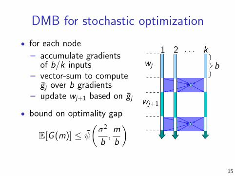
DMB for stochastic optimization
• for each node
– accumulate gradientsof b/k inputs
– vector-sum to computegj over b gradients
– update wj+1 based on gj
• bound on optimality gap
E[G (m)] ≤ ψ
(
σ2
b,m
b
)
1 2 . . . k
wj
wj+1
b
15

DMB for stochastic optimization
• if serial gap is ψ(σ2,m) = 2D2Lm
+ 2Dσ√m, then
E[G (m)] ≤ ψ
(
σ2
b,m
b
)
=2bD2L
m+
2Dσ√m
• parallel speed-up
S =m
mb
(
bk+ δ
) =k
1 + δbk
– asymptotic linear speed-up with b ∝ m1/3
– similar result for reaching same optimality gap
16

Web-scale experiments
• an online binary prediction problem
– predict highly monetizable queries– log of 109 queries issued to a commercial
search engine
• logistic loss function
f (w , z) = log(
1 + exp(−〈w , z〉))
• algorithm: stochastic dual averaging method(separate 5x10⁸ queries for parameter tuning)
17

Experiments: serial mini-batching
105
106
107
108
109
0.6
0.65
0.7
0.75
0.8
0.85
0.9
0.95
1
b=1b=32b=1024
number of inputs
averageloss
18
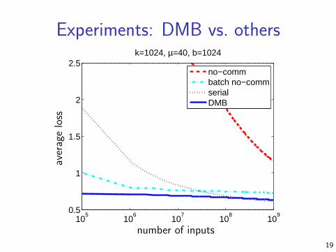
Experiments: DMB vs. others
105
106
107
108
109
0.5
1
1.5
2
2.5k=1024, µ=40, b=1024
no−commbatch no−commserialDMB
number of inputs
averageloss
19

Experiments: DMB vs. others
105
106
107
108
109
0.5
1
1.5
2
2.5k=32, µ=20, b=1024
no−commbatch no−commserialDMB
number of inputs
averageloss
20

Experiments: effects of latency
105
106
107
108
109
0.62
0.64
0.66
0.68
0.7
0.72
0.74
0.76b=1024
µ=40µ=320µ=1280µ=5120
number of inputs
averageloss
21

Experiments: optimal batch size
3 4 5 6 7 8 9 10 11 120.68
0.7
0.72
0.74
0.76
µ=20, m=107
log2(b)
3 4 5 6 7 8 9 10 11 12
0.66
0.68
0.7
0.72
0.74µ=20, m=108
log2(b)
3 4 5 6 7 8 9 10 11 120.61
0.62
0.63
0.64
0.65
0.66µ=20, m=109
log2(b)
• fixed cluster size k = 32 (latency µ = 20)
• empirical observations
– large batch size (b = 512) beneficial at first– small batch size (b = 128) better in the end
22

Summary
• distributed stochastic online prediction
– DMB turns serial algorithms into parallel ones– optimal O(
√m) regret bound for smooth loss
• stochastic optimization: near linear speed-up
• first provable demonstration that distributedcomputing worthwhile for these two problems
future directions
• DMB in asynchronous distributed environment(progress made, report available on arXiv)
• non-smooth functions? non-stochastic inputs?
23