IEEE TRANSACTIONS ON VEHICULAR TECHNOLOGY, VOL. 67, NO. 11, NOVEMBER 2018 10457

Optimal Design and Control of 4-IWD ElectricVehicles Based on a 14-DOF Vehicle ModelHuilong Yu , Member, IEEE, Federico Cheli, and Francesco Castelli-Dezza , Member, IEEE

Abstract—A 4-independent wheel driving (4-IWD) electric ve-hicle has distinctive advantages with both enhanced dynamic andenergy efficiency performances since this configuration providesmore flexibilities from both the design and control aspects. How-ever, it is difficult to achieve the optimal performances of a 4-IWDelectric vehicle with conventional design and control approaches.This paper is dedicated to investigating the vehicular optimal de-sign and control approaches, with a 4-IWD electric race car aimingat minimizing the lap time on a given circuit as a case study. A14-DOF vehicle model that can fully evaluate the influences ofthe unsprung mass is developed based on Lagrangian dynamics.The 14-DOF vehicle model implemented with the reprogrammedMagic Formula tire model and a time-efficient suspension modelsupports metric operations and parallel computing, which candramatically improve the computational efficiency. The optimaldesign and control problems with design parameters of the mo-tor, transmission, mass center, anti-roll bar and the suspension ofthe race car are successively formulated. The formulated prob-lems are subsequently solved by directly transcribing the originalproblems into large-scale nonlinear optimization problems basedon trapezoidal approach. The influences of the mounting positionsof the propulsion system, the mass and inertia of the unsprungmasses, the anti-roll bars, and suspensions on the lap time are ana-lyzed and compared quantitatively for the first time. Some interest-ing findings that are different from the ‘already known facts’ arepresented.

Index Terms—Vehicle dynamics, optimal design and control,4-IWD electric vehicles, unsprung mass, 14-DOF vehicle model.

I. INTRODUCTION

D EVELOPING electric vehicles (EVs) has been globallyrecognized as a promising solution to face the challenges

of air pollution, fossil oil crisis, and greenhouse gas emissions,which leads to mushroomed penetration of EVs in the lastdecade [1]. Most of the research interests on EVs are focused onenergy management [2], [3], electric motor control [4]–[6] and

Manuscript received March 25, 2018; revised July 12, 2018; accepted Septem-ber 2, 2018. Date of publication September 17, 2018; date of current versionNovember 12, 2018. The work of H. Yu is supported by the China ScholarshipCouncil. The review of this paper was coordinated by Dr. D. Cao. (Correspond-ing author: Federico Cheli.)

H. Yu was with the Department of Mechanical Engineering, Politecnico diMilano, Milano 20156, Italy. He is now with Vehicle Intelligence Pioneers Inc.,and also with Qingdao Academy of Intelligent Industries, Qingdao 266109, P.R.China (e-mail:,huilong.yu@ieee.org).

F. Cheli and F. Castelli Dezza are with the Department of MechanicalEngineering, Politecnico di Milano, 20156, Milano, Italy (e-mail:, federico.cheli@polimi.it; francesco.castellidezza@polimi.it).

Color versions of one or more of the figures in this paper are available onlineat http://ieeexplore.ieee.org.

Digital Object Identifier 10.1109/TVT.2018.2870673

dynamic control [7]–[9]. Continuous research on these topicshave improved the energy efficiency and dynamic performanceof the EVs a lot. However, optimal design and control of EVsthat can help to improve the performances further are seldomdiscussed in existing literature. With the fast advances in electricvehicles and the emerging autonomous electric vehicles, opti-mal control theory will undoubtedly play more important rolein realizing a ‘one line one design, one line one control’ conceptwith assist of the continuously reduced manufacturing cost, inwhich condition the optimality of the concerned performance ismore meaningful.

Normally, the proper parameters of the motor and transmis-sion are the primary considerations to meet the performancerequirements in electric vehicle design [10]. This is due to thefact that the power density, dynamic performance, energy ef-ficiency and cost of an electric powertrain rely heavily on thematching of the motor and transmission. However, most of theexisting work designed the electric powertrain following a con-ventional method which is unlikely to obtain the optimal per-formances [11]. This common approach can be summarizedinto three steps. The first step is to define the motor power ac-cording to the requirements on dynamic performance with asimplified point-mass vehicle model. Then the motor will bechosen from the available products of the manufacturers con-sidering the power density, cost, etc. The last step is to selectthe gearbox according to the torque-speed characteristics of themotor, the required maximum speed and the maximum torqueon the wheels. The limitations of the conventional approach are:(a) the most frequently employed simplified point-mass modelcan not predict the vehicle dynamic performances more pre-cisely, e.g., influences of the mounting positions of the electricmotors can not be evaluated, and the number of parameters canbe optimized is limited; (b) the optimal design solutions can notbe obtained with this manually design method. For a 4-IWDelectric vehicle, the motors and transmissions can be put on-board or in-wheel. However, the influences of their mountingpositions on the lap time have not been evaluated quantitativelyin the existing work. In addition, the chassis design which isknown to play a significant role in the vehicle dynamic per-formances [12]–[14], nonetheless, is mostly designed followingthe engineering experience based on manual calculation [15].There is a certain amount of existing work concerned the op-timal control problems of vehicles [16]–[18], however, vehicu-lar optimal design is seldom discussed. In model based designand control methodology, the modelling work serving as thebase is particularly of great significance, however, the mostly

0018-9545 © 2018 IEEE. Personal use is permitted, but republication/redistribution requires IEEE permission.See http://www.ieee.org/publications standards/publications/rights/index.html for more information.

10458 IEEE TRANSACTIONS ON VEHICULAR TECHNOLOGY, VOL. 67, NO. 11, NOVEMBER 2018

implemented 2-DOF, 3-DOF and 7-DOF vehicle models cannot represent the practical vehicle behavior precisely and it isonly possible to optimize limited number of parameters due totheir simplifications though they can save a lot of computingefforts [19].

This work aims to propose an optimal design approach toovercome the aforementioned drawbacks based on a developed14-DOF vehicle model with improved computing efficiency. Inparticular, the design of a 4-IWD electric race car aiming atminimizing the lap time on a given circuit is investigated as acase study. In order to test the performance of a design solution,a corresponding control strategy should be developed. However,there are various kinds of control approaches for electric vehicles[20]–[22] and accordingly, different control strategies may resultin different results even with the same designed race car. Thus,the optimal control of the electric race car is coupled into theoptimal design problem in this work which is reasonable inpractice. The final results will include both the optimal designand control solutions.

There novelty and original contributions of this work withrespect to the existing literature are presented as followings:First, a vectorized 14-DOF vehicle model that can fully evaluatethe influences of the unsprung mass is developed in MATLABbased on Lagrangian dynamics. In particular, the 14-DOF vehi-cle model is implemented with the reprogrammed full set MagicFormula tire model [23] that supports ‘.tir’ tire data file as inputand metric operations to improve the computation efficiency. Atime-efficient suspension model is also developed to describe therelationships between the wheel jounce and spring force, damp-ing force, toe angle, steering angle, camber angle, etc. Second,the optimal design and control problems with parameters of thepropulsion system, the mass center, the anti-roll bar and thesuspension of the electric race car as design parameters are suc-cessively formulated in standard formats based on the developed14-DOF vehicle model and a path following model in curvilin-ear coordinate system for the first time. Third, the complicatedlarge-scale optimal design and control problems based on the14-DOF vehicle model are solved based on direct transcriptionmethods for the first time with respect to the existing efforts.Fourth, results of different optimization cases and the influencesof the mounting positions of the propulsion system, the massand inertia variation of unsprung masses on the lap time are an-alyzed and compared quantitatively, which is rarely found in thesearch-able literature. Some new findings that are different fromthe facts that addressed by most engineers and researchers arepresented.

The remainder of this work is organized as follows.Section II details the formulation of the optimal design and con-trol problem, with the objective, variables and constraints arepresented. Section III elaborates the derivation and validation ofthe 14-DOF vehicle model in different maneuvers. Section IVdepicts briefly the employed numerical optimal control ap-proach, the simulation parameters and the optimization settings.Section V and Section VI demonstrated the obtained optimalparameters, coupled with trajectory, control and state variables.Results of different optimization cases are compared and ana-lyzed. Section VII concludes this work.

II. PROBLEM FORMULATION

This section gives an overall description of the optimal designand control problem. In this work, the objective is to minimizethe lap time tf :

J = min tf (1)

subject to:• the first order dynamic constraints

x(t) = f [x(t),u(t), t,p] (2)

• the boundaries of the state, control and design variables

xmin � x(t) � xmax

umin � u(t) � umax

pmin � p � pmax (3)

• the algebraic path constraints

gmin � g[x(t),u(t), t,p] � gmax (4)

• and the boundary conditions:

bmin � b[x(t0), t0,x(tf ), tf ,p] � bmax (5)

where x is the first order derivative of the state variables, f isthe dynamic model, x, u, p are respectively the state, controland design vector with their lower and upper bounds: xmin ,umin , pmin and xmax , umax , pmax . While g and b are the pathand boundary equations respectively with their lower and upperbounds gmin , bmin and gmax , bmax . The dimensions of the inputand output variables in Equations (2), (4) and (5) are separatelygiven as:

f : Rnx × Rnu × R × Rnp → Rnx

g : Rnx × Rnu × R × Rnp → Rng

b : Rnx × R × Rnx × R × Rnp → Rnb (6)

The state variables x, control variables u, design parametersp are described in the following paragraphs.

A. Variables

The state vector x includes the 14 DOF and their derivativesof the vehicle model, and 3 additional variables to describe thevehicle position in curvilinear coordinate system, so the numberof the state variables nx = 31 and x is denoted as:

x = {XA,b , YA,b , ZA,b , ϕ, φ, ψ, zf r , zf l , zrr , zr l ,

θf r , θf l , θrr , θr l , XA,b , YA,b , ZA,b , ϕ, φ, ψ,

zf r , zf l , zrr , zrl , θf r , θf l , θrr , θrl , s, n, χ} (7)

where XA,b , YA,b and ZA,b are the displacements of the masscenter in longitudinal, lateral and vertical directions of the globalreference system, ϕ, φ, and ψ are the roll angle, pitch angle andyaw angle of the vehicle body, zi and θi are the vertical androtational displacement of each wheel, s, n, χ are the traveleddistance, normal distance to the reference trajectory and orien-tation angle of the vehicle in the curvilinear coordinate system,

YU et al.: OPTIMAL DESIGN AND CONTROL OF 4-IWD ELECTRIC VEHICLES BASED ON A 14-DOF VEHICLE MODEL 10459

respectively. In this work, i = {fr, fl, rr, rl} means front right,front left, rear right and rear left.

The race car is assumed to be controlled with front wheelsteering and four independent wheel driving. The dynamicresponses of the steering system and the electric motors arenot taken into account in this study, the corresponding controlvector is:

u = [δ, Tf r , Tf l , Trr , Trl ], nu = 5 (8)

where δ is the steering angle, Ti is the driving/braking torqueacted on each wheel.

The design variables of the 4-IWD electric race car are pre-sented respectively in Section V and VI according to differentoptimization cases.

B. Algebraic Path Constraints

The algebraic path constraints are a set of constraints thatcan be denoted as functions of the state, control, final timeand design parameters. For the motor design, the maximumrotational speed Nmax,i should be constrained to a user setrange [clNm a x , cuNm a x ],

clNm a x ≤ Nmax = N bβ ≤ cuNm a x (9)

where Nb is the base speed and β is the constant power speedratio (CPSR) of each motor.

In order to let the motors work within their available operationzone, the motor speed Nm and output torque Tm should berespectively constrained within the user set lower and upperbounds:

clNcm≤ N cm = Nm − Nmax ≤ cuNcm

clTcm ≤ T cm = Tm − T max ≤ cuTcm (10)

where Ncm and Tcm are respectively the constraint functionrelated with the motor speed and torque, the units of torque,rotation speed, power are respectively Nm, rpm and kW , theavailable maximum torque of the motor is given as a function ofthe gear ratio ig , maximum power Pmax and the motor speed:

T max =

⎧⎪⎪⎨

⎪⎪⎩

9550igP max

N b, Nm ≤ N b

9550igP max

Nm, Nm > N b

(11)

The normal load F z, the tire slip κ, α and also should beconstrained within their allowable range:

cclFz ≤ F z ≤ cuFz

clκ ≤ κ ≤ cuκ

clα ≤ α ≤ cuα (12)

where cli and cui means the minimum and maximum value ofthe mentioned variables, respectively.

III. VEHICLE MODELLING

The configuration of the entire vehicle model is presentedin Fig. 1, where the interactions between the vehicle body,

Fig. 1. Vehicle model configuration.

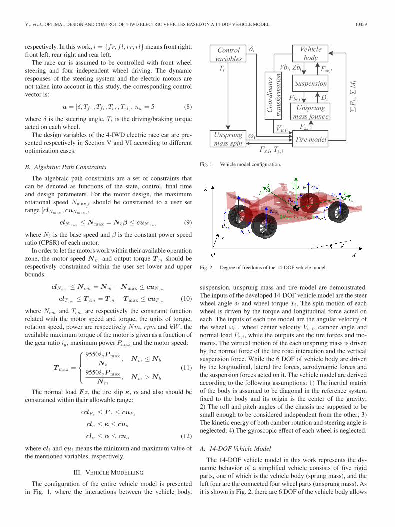
Fig. 2. Degree of freedoms of the 14-DOF vehicle model.

suspension, unsprung mass and tire model are demonstrated.The inputs of the developed 14-DOF vehicle model are the steerwheel angle δi and wheel torque Ti . The spin motion of eachwheel is driven by the torque and longitudinal force acted oneach. The inputs of each tire model are the angular velocity ofthe wheel ωi , wheel center velocity Vu,i , camber angle andnormal load Fz,i , while the outputs are the tire forces and mo-ments. The vertical motion of the each unsprung mass is drivenby the normal force of the tire road interaction and the verticalsuspension force. While the 6 DOF of vehicle body are drivenby the longitudinal, lateral tire forces, aerodynamic forces andthe suspension forces acted on it. The vehicle model are derivedaccording to the following assumptions: 1) The inertial matrixof the body is assumed to be diagonal in the reference systemfixed to the body and its origin is the center of the gravity;2) The roll and pitch angles of the chassis are supposed to besmall enough to be considered independent from the other; 3)The kinetic energy of both camber rotation and steering angle isneglected; 4) The gyroscopic effect of each wheel is neglected.

A. 14-DOF Vehicle Model

The 14-DOF vehicle model in this work represents the dy-namic behavior of a simplified vehicle consists of five rigidparts, one of which is the vehicle body (sprung mass), and theleft four are the connected four wheel parts (unsprung mass). Asit is shown in Fig. 2, there are 6 DOF of the vehicle body allows

10460 IEEE TRANSACTIONS ON VEHICULAR TECHNOLOGY, VOL. 67, NO. 11, NOVEMBER 2018

it to displace in the longitudinal, lateral and vertical directionas weel as to roll, pitch and yaw. In this work, the four wheelsare supposed to be fixed with the chassis to move in the longitu-dinal and lateral direction except their independent vertical androtational displacement. Thus, the 4 wheel parts have 2 DOFeach: one allows the wheel to move in vertical direction withregard to the vehicle body, and the other allows the wheel torotate around the axle.

The generalized coordinates are chosen and denoted withvector q:

q =

{qb

qu

}

=

{[XA,b , YA,b , ZA,b , ϕ, φ, ϕ]T

[θf r , θf l , θrr , θrl , zf r , zf l , zrr , zrl ]T

}

(13)

The corresponding velocity vector is presented as:

q =

{qb

qu

}

=

⎧⎨

⎩

[XA,b , YA,b , ZA,b , ϕ, φ, ϕ]T

[zf r , zf l , zrr , zr l , θf r , θf l , θrr , θr l ]T

⎫⎬

⎭

(14)

The relative position of the wheel center in XY plane of thevehicle reference frame [xw ,yw ] can be denoted as:

{xw

yw

}

=

⎧⎨

⎩

[lf , lf ,−lr ,−lr ]12[−wf ,wf ,−wr ,wr ]

⎫⎬

⎭(15)

where li and wi are respectively the x and y positions of eachwheel.

The vertical relative position of the unsprung mass zw inthe vehicle reference frame is denoted with its vertical zu , lon-gitudinal xw and lateral yw position in the vehicle referenceframe:

zw = zu − (ywϕ− xwφ+ ZA,b) (16)

the corresponding velocity of the unsprung mass in the vehiclereference frame can be denoted as:

zw = zu − (yw ϕ− xw φ+ ZA,b) (17)

The motion equations of the 14-DOF vehicle model can bederived based on the Lagrangian dynamics [24]:

⎧⎪⎪⎪⎨

⎪⎪⎪⎩

d

dt

(∂T

∂qb

)

− ∂T

∂qb= Qb

d

dt

(∂T

∂qu

)

− ∂T

∂qu= Qu

(18)

where T is the kinetic energy of the system, Qb and Qu arethe generalized forces applied on the sprung mass and unsprungmass respectively.

1) Kinetic Energy of the Sprung Mass: In order to fullyevaluate the influence of the unsprung mass, the wheels arefixed with the vehicle body in xb − yb directions. Based on thisconsideration, the kinetic energy of the sprung mass can be

denoted as:

Tb =12V T

b [Mb ]V b +∑ 1

2V T

u,i [Mu,i ]V u,i (19)

where the symbols in the above equation will be described inthe following paragraphs.

As shown in Fig. 2, there are two reference systems used inthis work: the global (inertia) reference system fixed with theground and the moving reference system fixed on the vehiclebody. The origin of the moving frame is located in the masscenter of the sprung mass, while the xb , yb and zb axles pointforward the longitudinal, lateral and vertical direction of motion.The two reference frame are connected with the transformationmatrix [hA,b ]:

[hA,b ] =

⎡

⎢⎢⎢⎢⎢⎢⎢⎢⎢⎣

cosψ sinψ 0 0 0 0

− sinψ cosψ 0 0 0 0

0 0 1 0 0 0

0 0 0 1 0 0

0 0 0 0 1 0

0 0 0 0 0 1

⎤

⎥⎥⎥⎥⎥⎥⎥⎥⎥⎦

(20)

The velocity of the vehicle body V b in the moving frame canthus be denoted as:

V b =

⎡

⎢⎢⎢⎢⎢⎢⎢⎢⎢⎣

Vxb

Vyb

Vzb

ωxb

ωyb

ωzb

⎤

⎥⎥⎥⎥⎥⎥⎥⎥⎥⎦

= [hA,b ]

⎡

⎢⎢⎢⎢⎢⎢⎢⎢⎢⎢⎣

XA,b

YA,b

ZA,b

ϕ

φ

ψ

⎤

⎥⎥⎥⎥⎥⎥⎥⎥⎥⎥⎦

= [hA,b ]qb (21)

The velocity V u,i of each unsprung mass is calculated withits relative position in the moving frame and the velocity vectorof the vehicle body, which can be denoted as:

V u,i =

[vux,i

vuy ,i

]

=

[1 0 0 0 zw,i −yw,i0 1 0 −zw,i 0 xw,i

]

V b

= [hb,u,i ][hA,b ]qb (22)

where vux,i and vuy ,i are, respectively, the longitudinal andlateral velocity of the unsprung mass in the moving frame, whilexw,i , yw,i and zw,i are the position coordinates of the unsprungmass in the moving frame denoted by Equation (15).

The mass matrix of the sprung mass [Mb ] and each unsprungmass [Mu,i ] are denoted as Equation (23) and Equation (24),

YU et al.: OPTIMAL DESIGN AND CONTROL OF 4-IWD ELECTRIC VEHICLES BASED ON A 14-DOF VEHICLE MODEL 10461

respectively.

[Mb ] = diag{mb,mb,mb, Jxxb , JyybJzzb} (23)

[Mu,i ] =

[mu,i 0

0 mu,i

]

(24)

where mb is the mass of the sprung mass, Jxxb , Jyyb and Jzzbare, respectively, the inertia of the sprung mass around theOb − xb , Ob − yb and Ob − zb axles.

With the above items, the kinetic energy of the sprung masscan be written in a more compact form:

Tb =12V T

b [Mb ]V b +∑ 1

2V T

u,i [Mu,i ]V u,i

=12qTb [hA,b ]T [Mb ][hA,b ]qb

+∑ 1

2qTb [hA,b ]

T [hb,u,i ]T [Mu,i ][hb,u,i ][hA,b ]qb

=12qTb [Mgb ]qb (25)

The generalized mass matrix [Mgb ] of the sprung mass is afunction of the generalized coordinates ZA,b , ψ and zu .

2) Kinetic Energy of the Unsprung Mass: The kinetic energyof the unsprung mass is composed by the vertical and rotationalmotion parts, which can be denoted as:

Tu =12ωTu [Ju ]ωu +

12V T

uz [Mu ]V uz (26)

In this work, the inertia of the propulsion system is taken intoaccount, the angular velocity ωu of the propulsion system andthe unsprung mass for an independent drive topology can bedenoted as:

ωu = [hu ][θf r , θf l , θrr , θr l

]T(27)

The transformation matrix [hu ] and the inertia matrix Ju aredenoted as:

⎧⎪⎨

⎪⎩

[hu ]=[diag{1, 1, 1, 1}; diag{ig ,f r , ig ,f l , ig ,rr , ig ,r l}]Ju =[diag{Ju,f r , Ju,f l , Ju,rr , Ju,rl , Jd,f r , Jd,f l ,

Jd,rr , Jd,r l}](28)

where Ju,i and Jd,i are respectively the inertia of each wheeland each motor, ig ,i is the speed ratio of each transmission.

The vertical velocity matrix V uz , and the mass matrix [Mu ]of the unsprung mass can be denoted as:

V uz = [zf r , zf l , zrr , zr l ]T (29)

[Mu ] = diag{mfr ,mf l ,mrr ,mrl} (30)

With the above terms, the kinetic energy of the unsprung massis denoted as Equation (31), and it can be derived as a function

Fig. 3. Vehicle model: forces and torque applied on the sprung mass.

Fig. 4. Vehicle model: forces and torque applied on the unsprung mass.

of the generalized coordinates and generalized mass matrix.

Tu =12ωTu [Ju ]ωu +

12V T

uz [Mu ]V uz

=12

⎡

⎢⎢⎢⎢⎣

θf r

θf l

θrr

θr l

⎤

⎥⎥⎥⎥⎦

T

[hu ]T [Ju ][hu ]

⎡

⎢⎢⎢⎢⎣

θf r

θf l

θrr

θr l

⎤

⎥⎥⎥⎥⎦

+12

⎡

⎢⎢⎢⎢⎣

zf r

zf l

zrr

zr l

⎤

⎥⎥⎥⎥⎦

T

[I]T [Mu ][I]

⎡

⎢⎢⎢⎢⎣

zf r

zf l

zrr

zr l

⎤

⎥⎥⎥⎥⎦

=12qTu [Mgu ]qu (31)

where [Mgu ] is the generalized unsprung mass collecting onlystatic values, it is denoted as:

[Mgu ] =

[[hu ]T [Ju ][hu ]

[Mu ]

]

(32)

3) Generalized Forces: The forces and torque acted on thesprung mass and unsprung mass are respectively illustrated asFig. 3 and Fig. 4. The vertical forces include the gravity ofthe sprung massmbg, the four suspension forces Fbs,i , the front

10462 IEEE TRANSACTIONS ON VEHICULAR TECHNOLOGY, VOL. 67, NO. 11, NOVEMBER 2018

and rear aerodynamic down forcesFdown,f andFdown,r , and theanti-roll forceFatr,i . Forces applied in the longitudinal directionare the four longitudinal tire forces Fx,i and the aerodynamicdrag force Fw . In lateral direction, there are only the four lateraltire forces Fy,i . The torque applied on the unsprung mass arefour driving/braking torque Td,i transmitted by the shafts. Theaerodynamic drag and down forces are presented as:

⎧⎪⎪⎨

⎪⎪⎩

Fdrag =12CdρAV

2x

Fdown,i =12Cl,iρAV

2x

(33)

where Cd is the drag coefficient, ρ is the air density, A is thevehicle effective area, Vx is the vehicle longitudinal velocity,Fdown,i is the aerodynamic downforce,Cl,i is the lift coefficient,i = {front, rear}.

The force matrix including the torque and forces applied onthe unsprung mass can be denoted as

F u =

⎡

⎢⎢⎢⎢⎢⎢⎢⎢⎢⎢⎢⎢⎢⎢⎢⎢⎢⎣

Td,f r +My,f r − Fx,f r zf r

Td,f l +My,f l − Fx,f lzf l

Td,rr +My,rr − Fx,rr zrr

Td,rl +My,rl − Fx,f r zrl

Fatr,f r − Fbs,f r + Fz,f r −mfrg

−Fatr,f l − Fbs,f l + Fz,f l −mf lg

Fatr,rr − Fbs,rr + Fz,rr −mrrg

−Fatr,r l − Fbs,rl + Fz,rl −mrlg

⎤

⎥⎥⎥⎥⎥⎥⎥⎥⎥⎥⎥⎥⎥⎥⎥⎥⎥⎦

(34)

where Td,i is the driving torque, My,i is the rolling resistancemoment, Fatr,i is the anti-roll force, Fz,i is the vertical forceacted on each tire and mi is the mass of each wheel.

The force matrix including the forces and torque acted on thesprung mass in each direction is denoted as Equation (35) asshown at the bottom of the page.

The generalized forces can be derived based on the forceanalysis and virtual work principle, which are presented in thefollowing equations. The similar detail derivation process can

be referred to [25].⎧⎪⎪⎨

⎪⎪⎩

Qb =∑

F∂rb∂qb

= F b

Qu =∑

F∂ru∂qu

= F u

(36)

4) Lagrange’s Equations: The generalized motion equa-tions of the rigid sprung and unsprung mass are derived inthe form of Equation (37) based on the Lagrangian mechanicsand D’Alembert’s principle. In this work, we differentiate thegeneralized mass matrix directly instead of calculating the par-tial differentials of the system kinetic energy to the time andgeneralized coordinates separately, qb and qu can be denoteddirectly based on Equation (37) and Equation (38) in this way,which is more efficient for derivation.

d

dt

(∂T

∂qb

)

− ∂T

∂qb= [Mgb ]qb + [Mgb ]qb

− 12qTb

[∂Mgb

∂qb

]

qb = Qb (37)

d

dt

(∂T

∂qu

)

− ∂T

∂qu= [Mgu ]qu + [Mgu ]qu

− 12qTb

[∂Mgb

∂qu

]

qb = Qu (38)

B. Suspension Model

The suspension model in this section involves the calculationof spring forces, damping forces, anti-roll forces, toe angles,camber angles and the steering angles. The suspension modelelaborated below is capable to describe the behavior of both thedependent and independent suspensions.

1) Spring and Damping Forces: The suspension force iscomposed by the spring force and damping force. When thestiffness and damping ratio are constant values, the suspensionforce can be denoted as Equation (39), the spring force on thespring is denoted as a function of the stiffness kbs,i and thedeformation lbs,i of the spring, while the damping force is afunction of damping cd,i and velocity ld,i of the damper.

Fbss,i = kbs,iΔls,i + cd,i ld,i (39)

The deformation of the spring travel Δls,i is a function ofwheel jounce ΔDi , which can be calculated by a transmission

F b=

⎡

⎢⎢⎢⎢⎢⎢⎢⎢⎢⎢⎢⎢⎢⎢⎣

∑(Fx,i cos δi − Fy,i sin δi) cosψ −∑ (Fx,i sin δi + Fy,i cos δi) sinψ − Fw cosψ

∑(Fx,i cos δi − Fy,i sin δi) sinψ +

∑(Fx,i sin δi + Fy,i cos δi) cosψ − Fw sinψ

∑Fbs,i −mg + Fdown,f + Fdown,r

−∑Fatr,iyu,i +∑Fbs,iyu,i +

∑(Fx,i sin δi + Fy,i cos δi)ZA,b +

∑Td,i sin δi

∑Fdown,ixu,i−

∑Fbs,ixu,i −

∑(Fx,i cos δi − Fy,i sin δi)ZA,b −

∑Td,i cos δi

∑Mz,i +

∑(Fx,i sin δi + Fy,i cos δi)xw,i −

∑(Fx,i cos δi − Fy,i sin δi)yw,i

⎤

⎥⎥⎥⎥⎥⎥⎥⎥⎥⎥⎥⎥⎥⎥⎦

(35)

YU et al.: OPTIMAL DESIGN AND CONTROL OF 4-IWD ELECTRIC VEHICLES BASED ON A 14-DOF VEHICLE MODEL 10463

ratio λs,i ,

Δls,i = λs,iΔDi (40)

where the wheel jounce ΔDi is the vertical movement of wheelor axle relative to the vehicle reference frame, which can bedefined as:

ΔDi = zw,i − zw0,i (41)

The deformation velocity of the damper can be denoted as:

ls,i = λs,i zw ,i (42)

where zw,i is the vertical position of the unsprung mass in themoving frame, zw0,i is its initial value.

Finally, the suspension force acted on each wheel can bedenoted as:

Fbs,i = λs,iFbss,i (43)

2) Anti-Roll Forces: In this work, the anti-roll bars are im-plemented to reduce the roll displacement of the race car duringfast cornering or over road irregularities. The anti-roll bar con-nects opposite left and right wheels together through a shortlever arm linked by a torsion spring. Taking the front axle as anexample, the anti-roll force Fatr,f is a function of the averagejounce Dl,f and delta jounce ΔDl,f of the left and right wheelsas denoted in Equation (44). The anti-roll forces can also be cal-culated with the given parameter tables and a 2-D interpretationmethod.

Fatr,f = f(Dl,f ,ΔDl,f ) (44)

where Dl,f = Dr , f +Dl , f

2 , ΔDl,f = Dr,f −Dl,f ,Dr,f andDl,f

are respectively the front wheel jounce of the right and left side.3) Camber Angles: The camber angle γi can be denoted as

a function of the wheel jounce and steering wheel angle inputby the driver,

γi = f(ΔDi, δdriver ) (45)

Similarly, the lookup table method based on the 2-D interpo-lation can be utilized to calculate the camber angle.

4) Toe Angles: Toe angle of each wheel ξi is also consideredin this suspension model, which is denoted as a function of thewheel jounce,

ξi = f(ΔDi) (46)

The toe angles can be calculated with the aforementioned 1-Dinterpolation method.

5) Steering Angles: The steering angle of each wheel δd,i onthe ground is expressed as a function of the wheel jounce andthe steering wheel angle input by the driver,

δd,i = f(ΔDi, δdriver ) (47)

A 2D interpolation method can be used in this model to obtainthe steering angle on the ground δd,i with the presented data.

The final steering angle on the ground in the vehicle referencesystem is:

δi = δd,i + ξi (48)

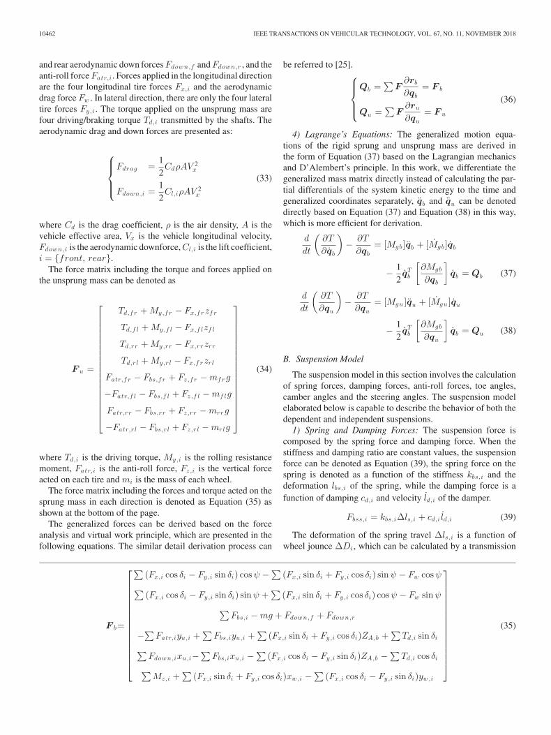
Fig. 5. Curvature of the track.

The tables describing all of the above relationships can beobtained via experiments in bench test for the interpretationmethod.

C. Tire Model

In this work, a semi-empirical tire model has been repro-grammed based on the full set of Magic Formula (MF) equa-tions in [26]. To improve the computation efficiency, the MF tiremodel is programmed in vector format in MATLAB. The longi-tudinal force Fx,i , lateral force Fy,i , overturning moment Mx,i ,rolling resistance moment My,i and aligning moment Mz,i ofthe tire are calculated with the vertical force Fz,i , longitudinalslip κi , side slip angle αi and inclination angle γi , forward ve-locity Vx as inputs, in this section i = {fr, fl, rr, rl} meansfront right, front left, rear right or rear left.

The Np pages of forces and torque can be calculated at onetime with high computational efficiency by the reprogrammedtire model:

[F x ,F y ,Mx ,M y ,M z ] = fT ire(F z ,κ,α,γ,V x) (49)

where the mapped dimensions of the input and output variablesare:

fT ire : R4×Np × R4×Np × R4×Np × R4×Np

× R1×Np → R20×Np

D. Path Following Model

1) Curvature of the Track: The curvature of the Nurburgringcircuit can be calculated by Equation (50) with the given X-Ycoordinates that can be obtained with GPS, or extracted andconverted from the commercial or open source map. The trackcan be described by its curvature and arc length in a curvilinearcoordinate system as it is presented in Fig. 5.

C =dx · ddy − ddx · dy

(√dx2 + dy2)

3 (50)

where dx, ddx, dy, ddy are the first and second order gradientsof the X-Y coordinates respectively.

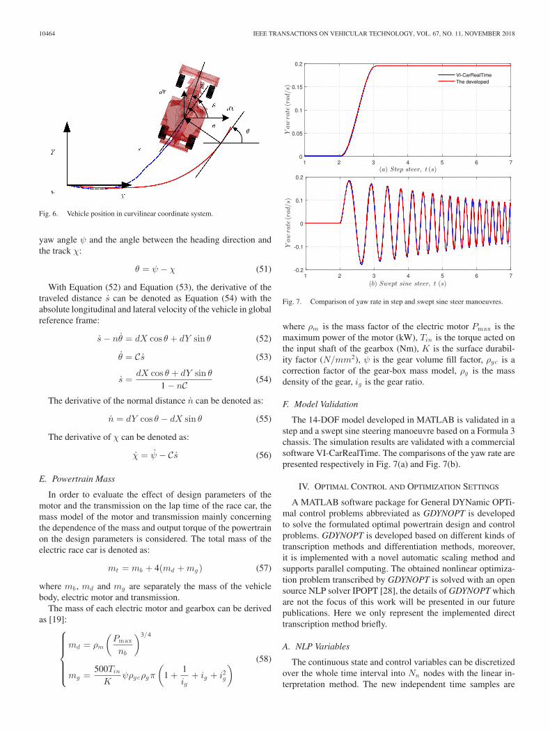
2) Vehicle Position in Curvilinear Coordinate System: Incurvilinear coordinate system shown in Fig. 6, the vehicularposition on the track can be described by its traveled distances along the reference trajectory, its normal distance to the ref-erence trajectory n, and its orientation angle θ at the currentposition [27]. The orientation angle can be denoted with the

10464 IEEE TRANSACTIONS ON VEHICULAR TECHNOLOGY, VOL. 67, NO. 11, NOVEMBER 2018

Fig. 6. Vehicle position in curvilinear coordinate system.

yaw angle ψ and the angle between the heading direction andthe track χ:

θ = ψ − χ (51)

With Equation (52) and Equation (53), the derivative of thetraveled distance s can be denoted as Equation (54) with theabsolute longitudinal and lateral velocity of the vehicle in globalreference frame:

s− nθ = dX cos θ + dY sin θ (52)

θ = Cs (53)

s =dX cos θ + dY sin θ

1 − nC (54)

The derivative of the normal distance n can be denoted as:

n = dY cos θ − dX sin θ (55)

The derivative of χ can be denoted as:

χ = ψ − Cs (56)

E. Powertrain Mass

In order to evaluate the effect of design parameters of themotor and the transmission on the lap time of the race car, themass model of the motor and transmission mainly concerningthe dependence of the mass and output torque of the powertrainon the design parameters is considered. The total mass of theelectric race car is denoted as:

mt = mb + 4(md +mg ) (57)

where mb , md and mg are separately the mass of the vehiclebody, electric motor and transmission.

The mass of each electric motor and gearbox can be derivedas [19]:

⎧⎪⎪⎪⎪⎨

⎪⎪⎪⎪⎩

md = ρm

(Pmax

nb

)3/4

mg =500TinK

ψρgcρgπ

(

1 +1ig

+ ig + i2g

) (58)

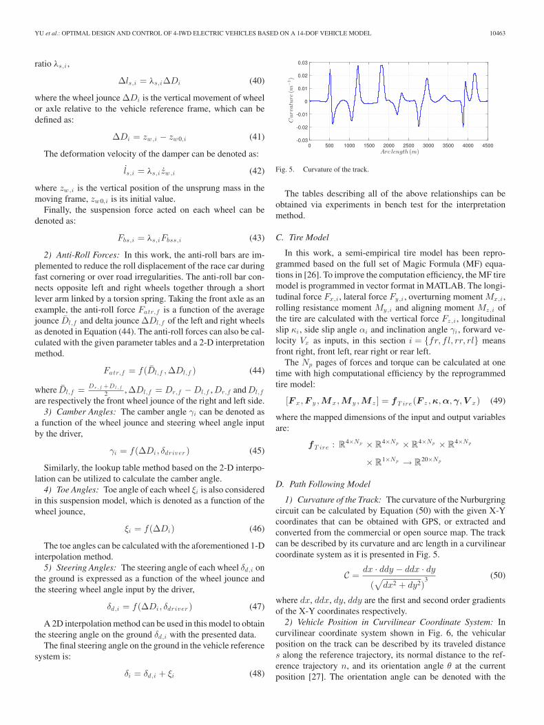
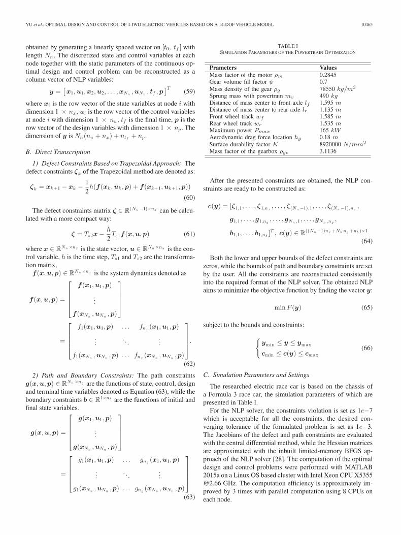
Fig. 7. Comparison of yaw rate in step and swept sine steer manoeuvres.

where ρm is the mass factor of the electric motor Pmax is themaximum power of the motor (kW), Tin is the torque acted onthe input shaft of the gearbox (Nm), K is the surface durabil-ity factor (N/mm2), ψ is the gear volume fill factor, ρgc is acorrection factor of the gear-box mass model, ρg is the massdensity of the gear, ig is the gear ratio.

F. Model Validation

The 14-DOF model developed in MATLAB is validated in astep and a swept sine steering manoeuvre based on a Formula 3chassis. The simulation results are validated with a commercialsoftware VI-CarRealTime. The comparisons of the yaw rate arepresented respectively in Fig. 7(a) and Fig. 7(b).

IV. OPTIMAL CONTROL AND OPTIMIZATION SETTINGS

A MATLAB software package for General DYNamic OPTi-mal control problems abbreviated as GDYNOPT is developedto solve the formulated optimal powertrain design and controlproblems. GDYNOPT is developed based on different kinds oftranscription methods and differentiation methods, moreover,it is implemented with a novel automatic scaling method andsupports parallel computing. The obtained nonlinear optimiza-tion problem transcribed by GDYNOPT is solved with an opensource NLP solver IPOPT [28], the details of GDYNOPT whichare not the focus of this work will be presented in our futurepublications. Here we only represent the implemented directtranscription method briefly.

A. NLP Variables

The continuous state and control variables can be discretizedover the whole time interval into Nn nodes with the linear in-terpretation method. The new independent time samples are

YU et al.: OPTIMAL DESIGN AND CONTROL OF 4-IWD ELECTRIC VEHICLES BASED ON A 14-DOF VEHICLE MODEL 10465

obtained by generating a linearly spaced vector on [t0, tf ] withlength Nn . The discretized state and control variables at eachnode together with the static parameters of the continuous op-timal design and control problem can be reconstructed as acolumn vector of NLP variables:

y =[x1,u1,x2,u2, . . . ,xNn

,uNn, tf ,p

]T(59)

where xi is the row vector of the state variables at node i withdimension 1 × nx , ui is the row vector of the control variablesat node i with dimension 1 × nu , tf is the final time, p is therow vector of the design variables with dimension 1 × np . Thedimension of y is Nn (nu + nx) + ntf + np .

B. Direct Transcription

1) Defect Constraints Based on Trapezoidal Approach: Thedefect constraints ζk of the Trapezoidal method are denoted as:

ζk = xk+1 − xk − 12h(f(xk ,uk ,p) + f(xk+1,uk+1,p))

(60)

The defect constraints matrix ζ ∈ R(Nn −1)×nx can be calcu-lated with a more compact way:

ζ = Ts2x − h

2Ts1f(x,u,p) (61)

where x ∈ RNn ×nx is the state vector, u ∈ RNn ×nu is the con-trol variable, h is the time step, Ts1 and Ts2 are the transforma-tion matrix,

f(x,u,p) ∈ RNn ×nx is the system dynamics denoted as

f(x,u,p) =

⎡

⎢⎢⎢⎣

f(x1,u1,p)

...

f(xNn,uNn

,p)

⎤

⎥⎥⎥⎦

=

⎡

⎢⎢⎢⎣

f1(x1,u1,p) . . . fnx (x1,u1,p)

.... . .

...

f1(xNn,uNn

,p) . . . fnx (xNn,uNn

,p)

⎤

⎥⎥⎥⎦.

(62)

2) Path and Boundary Constraints: The path constraintsg(x,u,p) ∈ RNn ×ng are the functions of state, control, designand terminal time variables denoted as Equation (63), while theboundary constraints b ∈ R1×nb are the functions of initial andfinal state variables.

g(x,u,p) =

⎡

⎢⎢⎢⎣

g(x1,u1,p)

...

g(xNn,uNn

,p)

⎤

⎥⎥⎥⎦

=

⎡

⎢⎢⎢⎣

g1(x1,u1,p) . . . gng (x1,u1,p)

.... . .

...

g1(xNn,uNn

,p) . . . gng (xNn,uNn

,p)

⎤

⎥⎥⎥⎦

(63)

TABLE ISIMULATION PARAMETERS OF THE POWERTRAIN OPTIMIZATION

After the presented constraints are obtained, the NLP con-straints are ready to be constructed as:

c(y) = [ζ1,1, . . . , ζ1,nx , . . . , ζ(Nn −1),1, . . . , ζ(Nn −1),nx ,

g1,1, . . . , g1,ng , . . . , gNn ,1, . . . , gNn ,ng ,

b1,1, . . . , b1,nb ]T , c(y) ∈ R((Nn −1)nx +Nn ng +nb )×1

(64)

Both the lower and upper bounds of the defect constraints arezeros, while the bounds of path and boundary constraints are setby the user. All the constraints are reconstructed consistentlyinto the required format of the NLP solver. The obtained NLPaims to minimize the objective function by finding the vector y:

minF (y) (65)

subject to the bounds and constraints:

{ymin ≤ y ≤ ymax

cmin ≤ c(y) ≤ cmax(66)

C. Simulation Parameters and Settings

The researched electric race car is based on the chassis ofa Formula 3 race car, the simulation parameters of which arepresented in Table I.

For the NLP solver, the constraints violation is set as 1e−7which is acceptable for all the constraints, the desired con-verging tolerance of the formulated problem is set as 1e−3.The Jacobians of the defect and path constraints are evaluatedwith the central differential method, while the Hessian matricesare approximated with the inbuilt limited-memory BFGS ap-proach of the NLP solver [28]. The computation of the optimaldesign and control problems were performed with MATLAB2015a on a Linux OS based cluster with Intel Xeon CPU X5355@2.66 GHz. The computation efficiency is approximately im-proved by 3 times with parallel computation using 8 CPUs oneach node.

10466 IEEE TRANSACTIONS ON VEHICULAR TECHNOLOGY, VOL. 67, NO. 11, NOVEMBER 2018

Fig. 8. The optimal racing line of 4-IWD electric race car.

Fig. 9. The optimal longitudinal velocity profile and steering wheel angle.

V. OPTIMAL POWERTRAIN DESIGN

A. Design Variables

The electric powertrain design in this work is implementedwith four uniform motors and single speed transmissions. Thebase speed nb and the constant power speed ratio (CPSR) βare selected as the design parameters of the motor. The envelopecurve of the torque-speed characteristics of the motor can beobtained with the two design parameters and the given maximumpower of the motor Pmax . The gear speed ratio ig is selected asthe design variable of each transmission. The powertrain designvector of the 4-IWD electric race car is:

p = [nb, β, ig ], np = 3 (67)

B. Design Results

The optimal racing line of the case with on-board motor isdemonstrated in Fig. 8, while Fig. 9 presents the longitudinalvelocity profile and optimal steering wheel angle respectively.

The optimal powertrain design results with the on-board andin-wheel motors are demonstrated in Table II. The interest-ing thing is that, the electric race car with 4 in-wheel motorscan achieve a better lap time performance. The improvementis 0. 281 s on the test track compared with the on-board motor

TABLE IIOPTIMAL POWERTRAIN DESIGN RESULTS

TABLE IIISENSITIVITY OF THE LAP TIME TO THE UNSPRUNG MASS

TABLE IVSENSITIVITY OF THE LAP TIME TO THE UNSPRUNG ROTATIONAL INERTIA

configuration. The influence of the unsprung mass on the laptime performance is a little different from the fact that addressedby most engineers and researchers. More research work shouldbe conducted to have a deep insight.

1) Sensitivity to the Unsprung Mass: In order to analyze theinfluence of increasing the unsprung mass of the 4-IWD electricrace car on the lap time performance, the powertrain parametersare fixed with the obtained ones in last section. Optimal controlwill be applied to find only the control parameters that minimiz-ing the lap time of the 4-IWD electric race car with differentunsprung mass. The obtained results are illustrated in Table III.In these three cases, different values of sprung mass are movedto the unsprung mass, while the rotational inertia is a uniformconstant value which can be realized by reasonably changingthe shape of the unsprung masses. It is illustrated in Table IIIthat when more unsprung mass is moved to the sprung mass,the lap time is decreased, which is different from the everybodyknows conclusions. The underlying reason will be analyzed andpresented in next section.

2) Sensitivity to the Unsprung Inertia: In this subsection,the unsprung mass is fixed and the lap time of race cars withdifferent unsprung rotational inertia are analyzed with optimalcontrol. As we can see from Table IV, the lap time performanceof the race car is very sensitive to the unsprung rotational inertia,which will get worse with the increasing of the rotational inertia.

VI. OPTIMAL CHASSIS DESIGN

The section will explore the influences of mass center, anti-roll bar and suspension on the lap time of the on-board 4-IWDelectric race car with the optimal control theory.

A. Optimization of the Mass Center

The mass center of the chassis is known to have signifi-cant influences on the lap time. Considering this, the distance

YU et al.: OPTIMAL DESIGN AND CONTROL OF 4-IWD ELECTRIC VEHICLES BASED ON A 14-DOF VEHICLE MODEL 10467

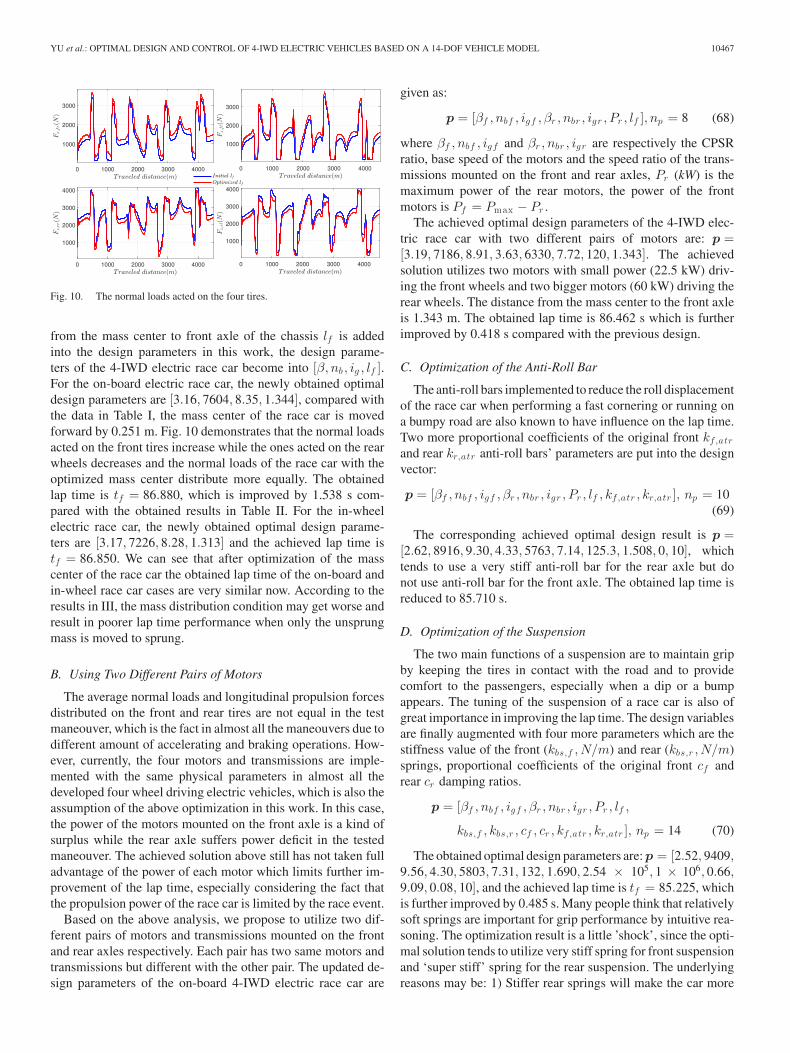
Fig. 10. The normal loads acted on the four tires.

from the mass center to front axle of the chassis lf is addedinto the design parameters in this work, the design parame-ters of the 4-IWD electric race car become into [β, nb , ig , lf ].For the on-board electric race car, the newly obtained optimaldesign parameters are [3.16, 7604, 8.35, 1.344], compared withthe data in Table I, the mass center of the race car is movedforward by 0.251 m. Fig. 10 demonstrates that the normal loadsacted on the front tires increase while the ones acted on the rearwheels decreases and the normal loads of the race car with theoptimized mass center distribute more equally. The obtainedlap time is tf = 86.880, which is improved by 1.538 s com-pared with the obtained results in Table II. For the in-wheelelectric race car, the newly obtained optimal design parame-ters are [3.17, 7226, 8.28, 1.313] and the achieved lap time istf = 86.850. We can see that after optimization of the masscenter of the race car the obtained lap time of the on-board andin-wheel race car cases are very similar now. According to theresults in III, the mass distribution condition may get worse andresult in poorer lap time performance when only the unsprungmass is moved to sprung.

B. Using Two Different Pairs of Motors

The average normal loads and longitudinal propulsion forcesdistributed on the front and rear tires are not equal in the testmaneouver, which is the fact in almost all the maneouvers due todifferent amount of accelerating and braking operations. How-ever, currently, the four motors and transmissions are imple-mented with the same physical parameters in almost all thedeveloped four wheel driving electric vehicles, which is also theassumption of the above optimization in this work. In this case,the power of the motors mounted on the front axle is a kind ofsurplus while the rear axle suffers power deficit in the testedmaneouver. The achieved solution above still has not taken fulladvantage of the power of each motor which limits further im-provement of the lap time, especially considering the fact thatthe propulsion power of the race car is limited by the race event.

Based on the above analysis, we propose to utilize two dif-ferent pairs of motors and transmissions mounted on the frontand rear axles respectively. Each pair has two same motors andtransmissions but different with the other pair. The updated de-sign parameters of the on-board 4-IWD electric race car are

given as:

p = [βf , nbf , igf , βr , nbr , igr , Pr , lf ], np = 8 (68)

where βf , nbf , igf and βr , nbr , igr are respectively the CPSRratio, base speed of the motors and the speed ratio of the trans-missions mounted on the front and rear axles, Pr (kW) is themaximum power of the rear motors, the power of the frontmotors is Pf = Pmax − Pr .

The achieved optimal design parameters of the 4-IWD elec-tric race car with two different pairs of motors are: p =[3.19, 7186, 8.91, 3.63, 6330, 7.72, 120, 1.343]. The achievedsolution utilizes two motors with small power (22.5 kW) driv-ing the front wheels and two bigger motors (60 kW) driving therear wheels. The distance from the mass center to the front axleis 1.343 m. The obtained lap time is 86.462 s which is furtherimproved by 0.418 s compared with the previous design.

C. Optimization of the Anti-Roll Bar

The anti-roll bars implemented to reduce the roll displacementof the race car when performing a fast cornering or running ona bumpy road are also known to have influence on the lap time.Two more proportional coefficients of the original front kf,atrand rear kr,atr anti-roll bars’ parameters are put into the designvector:

p = [βf , nbf , igf , βr , nbr , igr , Pr , lf , kf,atr , kr,atr ], np = 10(69)

The corresponding achieved optimal design result is p =[2.62, 8916, 9.30, 4.33, 5763, 7.14, 125.3, 1.508, 0, 10], whichtends to use a very stiff anti-roll bar for the rear axle but donot use anti-roll bar for the front axle. The obtained lap time isreduced to 85.710 s.

D. Optimization of the Suspension

The two main functions of a suspension are to maintain gripby keeping the tires in contact with the road and to providecomfort to the passengers, especially when a dip or a bumpappears. The tuning of the suspension of a race car is also ofgreat importance in improving the lap time. The design variablesare finally augmented with four more parameters which are thestiffness value of the front (kbs,f , N/m) and rear (kbs,r , N/m)springs, proportional coefficients of the original front cf andrear cr damping ratios.

p = [βf , nbf , igf , βr , nbr , igr , Pr , lf ,

kbs,f , kbs,r , cf , cr , kf,atr , kr,atr ], np = 14 (70)

The obtained optimal design parameters are: p = [2.52, 9409,9.56, 4.30, 5803, 7.31, 132, 1.690, 2.54 × 105, 1 × 106, 0.66,9.09, 0.08, 10], and the achieved lap time is tf = 85.225, whichis further improved by 0.485 s. Many people think that relativelysoft springs are important for grip performance by intuitive rea-soning. The optimization result is a little ’shock’, since the opti-mal solution tends to utilize very stiff spring for front suspensionand ‘super stiff’ spring for the rear suspension. The underlyingreasons may be: 1) Stiffer rear springs will make the car more

10468 IEEE TRANSACTIONS ON VEHICULAR TECHNOLOGY, VOL. 67, NO. 11, NOVEMBER 2018

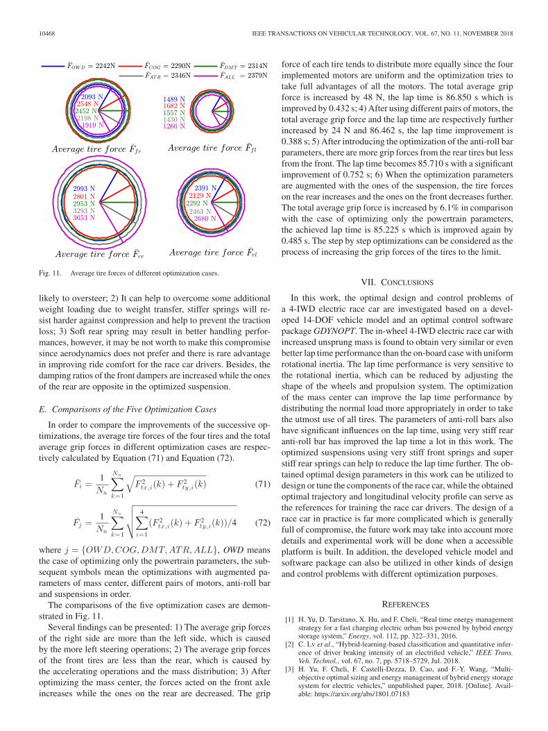
Fig. 11. Average tire forces of different optimization cases.

likely to oversteer; 2) It can help to overcome some additionalweight loading due to weight transfer, stiffer springs will re-sist harder against compression and help to prevent the tractionloss; 3) Soft rear spring may result in better handling perfor-mances, however, it may be not worth to make this compromisesince aerodynamics does not prefer and there is rare advantagein improving ride comfort for the race car drivers. Besides, thedamping ratios of the front dampers are increased while the onesof the rear are opposite in the optimized suspension.

E. Comparisons of the Five Optimization Cases

In order to compare the improvements of the successive op-timizations, the average tire forces of the four tires and the totalaverage grip forces in different optimization cases are respec-tively calculated by Equation (71) and Equation (72).

Fi =1Nn

Nn∑

k=1

√

F 2tx,i(k) + F 2

ty ,i(k) (71)

Fj =1Nn

Nn∑

k=1

√√√√

4∑

i=1

(F 2tx,i(k) + F 2

ty ,i(k))/4 (72)

where j = {OWD,COG,DMT,ATR,ALL}, OWD meansthe case of optimizing only the powertrain parameters, the sub-sequent symbols mean the optimizations with augmented pa-rameters of mass center, different pairs of motors, anti-roll barand suspensions in order.

The comparisons of the five optimization cases are demon-strated in Fig. 11.

Several findings can be presented: 1) The average grip forcesof the right side are more than the left side, which is causedby the more left steering operations; 2) The average grip forcesof the front tires are less than the rear, which is caused bythe accelerating operations and the mass distribution; 3) Afteroptimizing the mass center, the forces acted on the front axleincreases while the ones on the rear are decreased. The grip

force of each tire tends to distribute more equally since the fourimplemented motors are uniform and the optimization tries totake full advantages of all the motors. The total average gripforce is increased by 48 N, the lap time is 86.850 s which isimproved by 0.432 s; 4) After using different pairs of motors, thetotal average grip force and the lap time are respectively furtherincreased by 24 N and 86.462 s, the lap time improvement is0.388 s; 5) After introducing the optimization of the anti-roll barparameters, there are more grip forces from the rear tires but lessfrom the front. The lap time becomes 85.710 s with a significantimprovement of 0.752 s; 6) When the optimization parametersare augmented with the ones of the suspension, the tire forceson the rear increases and the ones on the front decreases further.The total average grip force is increased by 6.1% in comparisonwith the case of optimizing only the powertrain parameters,the achieved lap time is 85.225 s which is improved again by0.485 s. The step by step optimizations can be considered as theprocess of increasing the grip forces of the tires to the limit.

VII. CONCLUSIONS

In this work, the optimal design and control problems ofa 4-IWD electric race car are investigated based on a devel-oped 14-DOF vehicle model and an optimal control softwarepackage GDYNOPT. The in-wheel 4-IWD electric race car withincreased unsprung mass is found to obtain very similar or evenbetter lap time performance than the on-board case with uniformrotational inertia. The lap time performance is very sensitive tothe rotational inertia, which can be reduced by adjusting theshape of the wheels and propulsion system. The optimizationof the mass center can improve the lap time performance bydistributing the normal load more appropriately in order to takethe utmost use of all tires. The parameters of anti-roll bars alsohave significant influences on the lap time, using very stiff rearanti-roll bar has improved the lap time a lot in this work. Theoptimized suspensions using very stiff front springs and superstiff rear springs can help to reduce the lap time further. The ob-tained optimal design parameters in this work can be utilized todesign or tune the components of the race car, while the obtainedoptimal trajectory and longitudinal velocity profile can serve asthe references for training the race car drivers. The design of arace car in practice is far more complicated which is generallyfull of compromise, the future work may take into account moredetails and experimental work will be done when a accessibleplatform is built. In addition, the developed vehicle model andsoftware package can also be utilized in other kinds of designand control problems with different optimization purposes.

REFERENCES

[1] H. Yu, D. Tarsitano, X. Hu, and F. Cheli, “Real time energy managementstrategy for a fast charging electric urban bus powered by hybrid energystorage system,” Energy, vol. 112, pp. 322–331, 2016.

[2] C. Lv et al., “Hybrid-learning-based classification and quantitative infer-ence of driver braking intensity of an electrified vehicle,” IEEE Trans.Veh. Technol., vol. 67, no. 7, pp. 5718–5729, Jul. 2018.

[3] H. Yu, F. Cheli, F. Castelli-Dezza, D. Cao, and F.-Y. Wang, “Multi-objective optimal sizing and energy management of hybrid energy storagesystem for electric vehicles,” unpublished paper, 2018. [Online]. Avail-able: https://arxiv.org/abs/1801.07183

YU et al.: OPTIMAL DESIGN AND CONTROL OF 4-IWD ELECTRIC VEHICLES BASED ON A 14-DOF VEHICLE MODEL 10469

[4] C. Lv, Y. Liu, X. Hu, H. Guo, D. Cao, and F.-Y. Wang, “Simultaneousobservation of hybrid states for cyber-physical systems: A case study ofelectric vehicle powertrain,” IEEE Trans. Cybern., vol. 48, no. 8, pp. 2357–2367, Aug. 2018.

[5] Y.-S. Lin, K.-W. Hu, T.-H. Yeh, and C.-M. Liaw, “An electric-vehicleIPMSM drive with interleaved front-end DC/DC converter,” IEEE Trans.Veh. Technol., vol. 65, no. 6, pp. 4493–4504, Jun. 2016.

[6] C. Lv et al., “Characterization of driver neuromuscular dynamicsfor human-automation collaboration design of automated vehicles,”IEEE/ASME Trans. Mechatronics, 2018, p. 1.

[7] L. Zhai, T. Sun, and J. Wang, “Electronic stability control based on motordriving and braking torque distribution for a four in-wheel motor driveelectric vehicle,” IEEE Trans. Veh. Technol., vol. 65, no. 6, pp. 4726–4739, Jun. 2016.

[8] J. S. Hu, Y. Wang, H. Fujimoto, and Y. Hori, “Robust yaw stability controlfor in-wheel motor electric vehicles,” IEEE/ASME Trans. Mechatronics,vol. 22, no. 3, pp. 1360–1370, Jun. 2017.

[9] M. S. Basrah, E. Siampis, E. Velenis, D. Cao, and S. Longo, “Wheel slipcontrol with torque blending using linear and nonlinear model predictivecontrol,” Veh. Syst. Dyn., vol. 55, no. 11, pp. 1665–1685, 2017.

[10] M. Ehsani, Y. Gao, and A. Emadi, Modern Electric, Hybrid Electric, andFuel Cell Vehicles: Fundamentals, Theory, and Design. Boca Raton, FL,USA: CRC Press, 2009.

[11] S. Soylu, Electric Vehicles—Modelling and Simulations. Rijeka, Croatia:InTech Europe, 2011.

[12] W. Milliken and D. Milliken, Race Car Vehicle Dynamics (ser. PremiereSeries). Warrendale, PA, USA: SAE International, 1995.

[13] D. Cao, X. Song, and M. Ahmadian, “Editors’ perspectives: road vehiclesuspension design, dynamics, and control,” Veh. Syst. Dynamics, vol. 49,no. 1/2, pp. 3–28, 2011.

[14] Z. Yin, A. Khajepour, D. Cao, B. Ebrahimi, and K. Guo, “A new pneu-matic suspension system with independent stiffness and ride height tuningcapabilities,” Veh. Syst. Dyn., vol. 50, no. 12, pp. 1735–1746, 2012.

[15] W. Milliken, D. Milliken, M. Olley, and Society of Automotive Engineers,Chassis Design: Principles and Analysis (ser. Premiere Series Bks). War-rendale, PA, USA: SAE International, 2002.

[16] E. N. Smith, E. Velenis, D. Tavernini, and D. Cao, “Effect of handlingcharacteristics on minimum time cornering with torque vectoring,” Veh.Syst. Dyn., vol. 56, no. 2, pp. 221–248, 2018.

[17] R. Lot and N. Dal Bianco, “The significance of high-order dynamics inlap time simulations,” in The Dynamics of Vehicles on Roads and Tracks:Proceedings of the 24th Symposium of the International Association forVehicle System Dynamics (IAVSD 2015), Graz, Austria, 17-21 August2015. Boca Raton, FL, USA: CRC Press, 2016, pp. 553–562.

[18] D. J. N. Limebeer and G. Perantoni, “Optimal control of a formula onecar on a three-dimensional track part 2: Optimal control,” J. Dyn. Syst.,Measure., Control, vol. 137, no. 5, May 2015, Art. no. 051019.

[19] H. Yu, F. Castelli-Dezza, and F. Cheli, “Optimal powertrain design andcontrol of a 2-IWD electric race car,” in Proc. Int. Conf. Elect. Electron.Technol. Automot., 2017, pp. 1–7.

[20] F. Braghin and E. Sabbioni, “A 4WS control strategy for improving racecar performances,” in Proc. ASME 8th Biennial Conf. Eng. Syst. DesignAnal., 2006, pp. 297–304.

[21] F. Cheli, S. Melzi, E. Sabbioni, and M. Vignati, “Torque vectoring controlof a four independent wheel drive,” in Proc. ASME Int. Design Eng. Tech.Conf. Comput. Inf. Eng. Conf., 2013, pp. 1–8.

[22] L. De Novellis, A. Sorniotti, and P. Gruber, “Wheel torque distributioncriteria for electric vehicles with torque-vectoring differentials,” IEEETrans. Veh. Technol., vol. 63, no. 4, pp. 1593–1602, 2014.

[23] Hans B. Pacejka, Tyre and Vehicle Dynamics, 2nd Ed. Oxford, U.K.:Butterworth-Heinemann, 2006.

[24] F. Cheli and G. Diana, Advanced Dynamics of Mechanical Systems. Berlin,Germany: Springer-Verlag, 2015.

[25] F. Cheli, E. Leo, S. Melzi, and F. Mancosu, “A 14dof model for theevaluation of vehicle dynamics: numerical experimental comparison,” Int.J. Mech. Control, vol. 6, no. 2, pp. 19–30, 2006.

[26] I. J. Besselink, a. J. Schmeitz, and H. B. Pacejka, “An improved MagicFormula/Swift tyre model that can handle inflation pressure changes,” Veh.Syst. Dyn., vol. 48, no. 1, pp. 337–352, 2010.

[27] R. Lot and F. Biral, “A curvilinear abscissa approach for the lap timeoptimization of racing vehicles,” IFAC Proc. Vol., vol. 19, pp. 7559–7565,2014.

[28] A. Wachter and L. T. Biegler, “On the implementation of an interior-pointfilter line-search algorithm for large-scale nonlinear programming,” Math.Program., vol. 106, no. 1, pp. 25–57, 2006.

Huilong Yu (M’17) received the M.Sc. degree inmechanical engineering from the Beijing Institute ofTechnology, Beijing, China, and the Ph.D. degree inmechanical engineering from the Politecnico diMilano, Milano, Italy, in 2013 and 2017, respectively.He is currently a Research Fellow of advanced vehicleengineering with the University of Waterloo, Water-loo, ON, Canada. His research interests include ve-hicle dynamics, optimal control, closed-loop control,and energy management problems of conventional,electric, hybrid electric, and autonomous vehicles.

Federico Cheli received the Graduate degree in me-chanical engineering from the Politecnico di Milano,Milano, Italy, in 1981. He is currently a Full Profes-sor with the Department of Mechanics, Politecnicodi Milano. From 1992 to 2000, he was an AssociateProfessor with the Faculty of Industrial Engineering,Politecnico di Milano. He is the Co-founder of theE_CO spin-off and an author of more than 380 publi-cations in international journals or presented at inter-national conferences. His scientific activity concernsresearch on vehicle performance, handling and com-

fort problems, active control, ADAS, and electric and autonomous vehicles.He is a member of the editorial board of the International Journal of Vehi-cle Performance and International Journal of Vehicle Systems Modeling andTesting.

Francesco Castelli-Dezza (M’94) received theM.Sc. and Ph.D. degrees in electrical engineeringfrom the Politecnico di Milano, Milano, Italy, in 1986and 1990, respectively. He is currently a Full Profes-sor with the Department of Mechanical Engineering,Politecnico di Milano. His research interests includestudies on dynamic behavior of electrical machines,electrical drives control and design, and power elec-tronics for energy flow management. He is a memberof the IEEE Power Electronics Society.