Optimal Control Simulation Problem -...

ECE-S642-601 Midterm 1 Solutions Fall 2009

page 1 of 21

ECE-S642 001 Optimal Control Midterm

This solution was prepared by Rob Allen on Feb 9, 2009

The basic questions are given on the following page the solution presented includes a variety of {Q, R}

which include the values in our exam

Optimal Control Simulation Problem


page 2 of 21

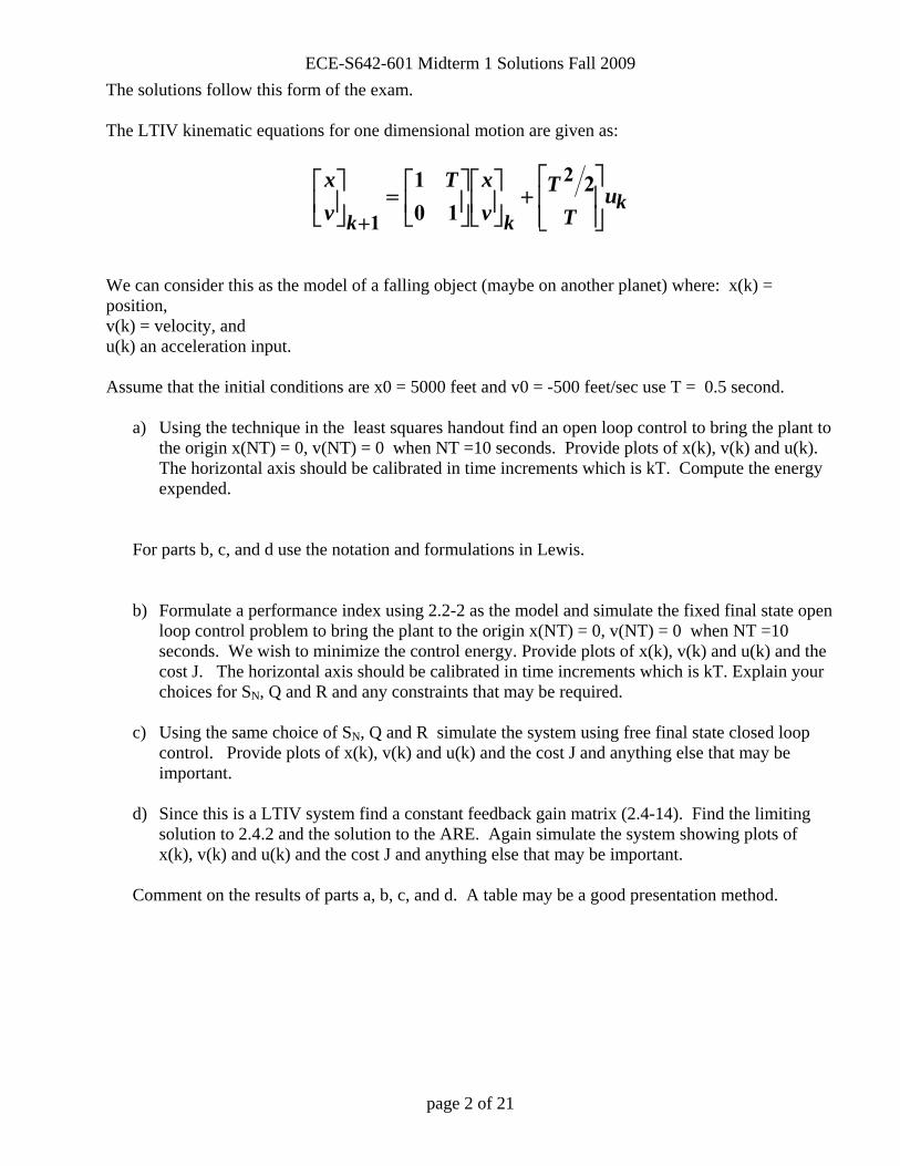
The solutions follow this form of the exam. The LTIV kinematic equations for one dimensional motion are given as:

kkk

uT

TvxT

vx

⎥⎥⎦

⎤

⎢⎢⎣

⎡+⎥

⎦

⎤⎢⎣

⎡⎥⎦

⎤⎢⎣

⎡=⎥

⎦

⎤⎢⎣

⎡

+

210

1 2

1

We can consider this as the model of a falling object (maybe on another planet) where: x(k) = position, v(k) = velocity, and u(k) an acceleration input. Assume that the initial conditions are x0 = 5000 feet and v0 = -500 feet/sec use T = 0.5 second.

a) Using the technique in the least squares handout find an open loop control to bring the plant to the origin x(NT) = 0, v(NT) = 0 when NT =10 seconds. Provide plots of x(k), v(k) and u(k). The horizontal axis should be calibrated in time increments which is kT. Compute the energy expended.

For parts b, c, and d use the notation and formulations in Lewis. b) Formulate a performance index using 2.2-2 as the model and simulate the fixed final state open

loop control problem to bring the plant to the origin x(NT) = 0, v(NT) = 0 when NT =10 seconds. We wish to minimize the control energy. Provide plots of x(k), v(k) and u(k) and the cost J. The horizontal axis should be calibrated in time increments which is kT. Explain your choices for SN, Q and R and any constraints that may be required.

c) Using the same choice of SN, Q and R simulate the system using free final state closed loop

control. Provide plots of x(k), v(k) and u(k) and the cost J and anything else that may be important.

d) Since this is a LTIV system find a constant feedback gain matrix (2.4-14). Find the limiting

solution to 2.4.2 and the solution to the ARE. Again simulate the system showing plots of x(k), v(k) and u(k) and the cost J and anything else that may be important.

Comment on the results of parts a, b, c, and d. A table may be a good presentation method.


page 3 of 21

Given Problem:

Part (a)

Solution As stated in the least squares handout when driving a discrete time system to the origin in k>n steps, there are many solutions. The problem is underdetermined, in that there are n equations, or constraints, specified by the physics of the problem with k unknowns (discrete control inputs). The numbers of unknowns are specified by the finite time specified to drive the system from an initial state to the origin. What follows is an attempt to show that the pseudo-inverse1 can be thought of a constrained minimum energy optimization problem and can be turned into an unconstrained optimization problem using Hamiltonian based approach taught in this course. The results here will be utilized in the discussion to compare simulation results from least squares and fixed-final state open loop control methods. As shown in the handout the problem can be written as Y = CT U (1) The Euclidian, or 2-norm can be thought of as the square root of the total energy in a signal. Let the cost function, or performance index, be the square of the 2-norm of the control energy

( ) ( )...... 23

22

21

223

22

21

2

2+++=+++== uuuuuuUJ (2)

Now constrain U so that it must also satisfy the physics of the problem, which are specified by a system of discrete time equations, with initial and terminal conditions, as in the handout,


page 4 of 21

Y – CT U = 0 (3) To transform this problem into an unconstrained optimization problem, introduce the Hamiltonian (scalar function) as

H = || U ||2 - λΤ ( Y – CT U) (4) where λ is a Lagrangian multiplier. To be a stationary point, a necessary condition is that

0λCUU

TT =−=

∂∂ 2H (5)

Multiplying both sides by CT and using (1) enables the solution for λ to be written as

YC(Cλ TTT

1)2 −= (6) Plugging this into (5) and solving for U, yields

YC(CCU TTT

TT

1)−= (7) The handout refers to the terms proceeding the Y term as a pseudo-inverse.

]) 1−TTT

TT C(C[C (8)

To check that the solution for U is indeed a minimum, the Hessian must be positive definite. The Hessian is,

022

>=∂∂

2UH (9)

Thus, the pseudo inverse solution for U, minimizes the control energy required to take the system from x0 to xN in k steps (k>n). Simulation results are shown on the following page. Note what might be a drawback to this method is that although the control energy is minimized, large state excursions are not penalized. For example at 0.5 seconds till the object lands, the object is traveling at approximately 100 feet per second and undergoing rapid deceleration!


page 5 of 21

Figure 1 Open-loop least squares solution for discrete time model of falling object.

Figure 2. Cost of least squares solution as a function of time. Total cost or control energy expended is 100188. Note here that the cost used includes a ½ so another acceptable answer is 200376


page 6 of 21

Part (b)

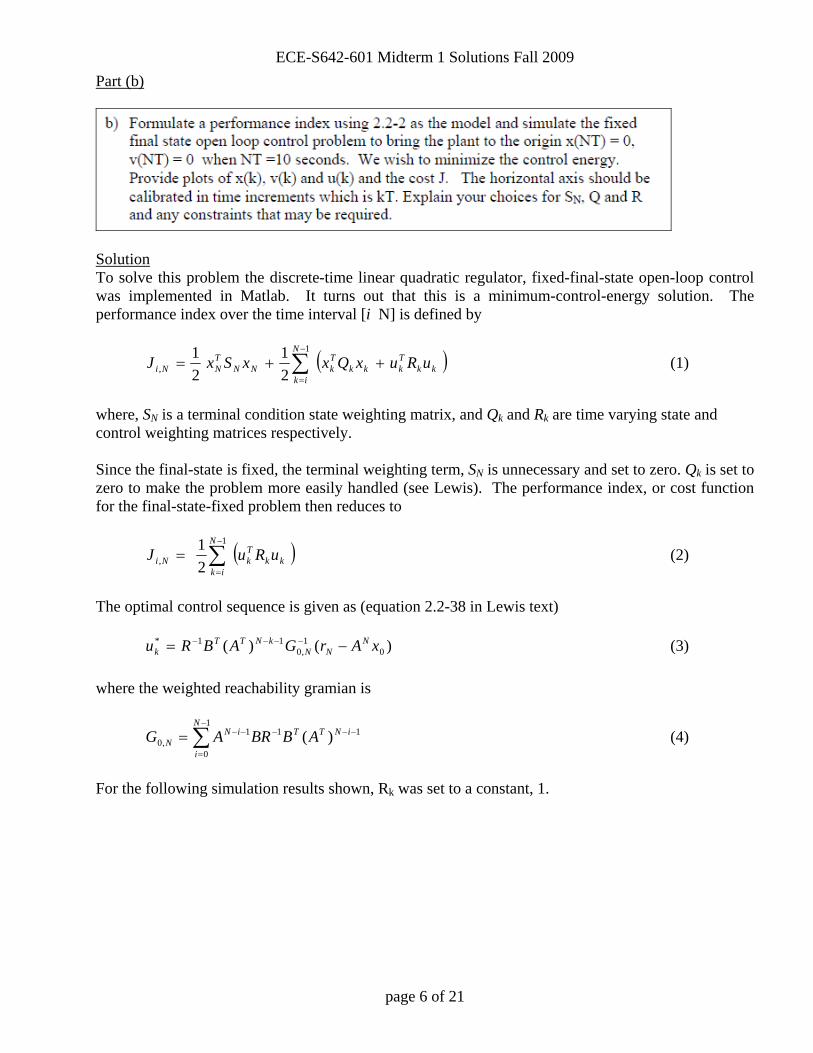
Solution To solve this problem the discrete-time linear quadratic regulator, fixed-final-state open-loop control was implemented in Matlab. It turns out that this is a minimum-control-energy solution. The performance index over the time interval [i N] is defined by

( )∑−

=

++=1

, 21

21 N

ikkk

Tkkk

TkNN

TNNi uRuxQxxSxJ (1)

where, SN is a terminal condition state weighting matrix, and Qk and Rk are time varying state and control weighting matrices respectively. Since the final-state is fixed, the terminal weighting term, SN is unnecessary and set to zero. Qk is set to zero to make the problem more easily handled (see Lewis). The performance index, or cost function for the final-state-fixed problem then reduces to

( )∑−

=

=1

, 21 N

ikkk

TkNi uRuJ (2)

The optimal control sequence is given as (equation 2.2-38 in Lewis text) )()( 0

1,0

11* xArGABRu NNN

kNTTk −= −−−− (3)

where the weighted reachability gramian is

∑−

=

−−−−−=1

0

111,0 )(

N

i

iNTTiNN ABBRAG (4)

For the following simulation results shown, Rk was set to a constant, 1.


page 7 of 21

Figure 3 Fixed-final-state open-loop control simulation results for discrete time model of a falling object.

Figure 4 Cost of least fixed-final-state solution as a function of time. Total cost or energy expended is 100188, which is the same as the least squares solution.


page 8 of 21

Part (c)

Solution To solve this problem the discrete-time linear quadratic regulator, free-final-state closed-loop control simulation routine was implemented in Matlab (see Appendix).

[x,u,K,S,J]= dlqropt(A,B,Q,R,sN,x0,N); The cost function is

( )∑−

=

++=1

, 21

21 N

ikkk

Tkkk

TkNN

TNNi uRuxQxxSxJ (1)

and the equation to solve for the optimal time-varying feedback is

kkk xKu −= (2) where the time varying gain is given by

kkTkkkk

Tkk ASBRBSBK 1

11 )( +

−+ += (3)

and the cost kernel is given by the following Riccati equation

[ ] kkkTkkkk

Tkkkk

Tkk QASBRBSBBSSAS ++−= +

−+++ 1

1111 )( (4)

To implement these equations the cost kernel (4) and time varying state feedback gain (3) are computed beforehand and stored off-line. The cost kernel (4) must be solved backwards in time, with an initial condition of SN which is specified by the designer. After (3) and (4) are solved the governing discrete time state equations are solved forwards in time, utilizing the optimal time varying feedback gain to compute the optimal control input at each time. These are referred to as on-line, computations in the textbook (Lewis). To learn about the behavior of the weighting matrices in the cost equation (1), some limiting cases are presented. Zero-Input-Response(ZIR) Now that the boundary condition of a fixed final state has been removed that existed in the least squares and fixed-final-state solutions, the final-free-state closed loop solution can minimize control energy with no constraints. As an extreme example, setting Q = SN = 0 and R very small will effectively have zero control energy and yields the Zero Input Response (ZIR) of the system.


page 9 of 21

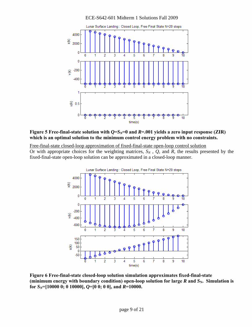
Figure 5 Free-final-state solution with Q=SN=0 and R=.001 yields a zero input response (ZIR) which is an optimal solution to the minimum control energy problem with no constraints. Free-final-state closed-loop approximation of fixed-final-state open-loop control solution Or with appropriate choices for the weighting matrices, SN , Q, and R, the results presented by the fixed-final-state open-loop solution can be approximated in a closed-loop manner.

Figure 6 Free-final-state closed-loop solution simulation approximates fixed-final-state (minimum energy with boundary condition) open-loop solution for large R and SN. Simulation is for SN=[10000 0; 0 10000], Q=[0 0; 0 0], and R=10000.


page 10 of 21

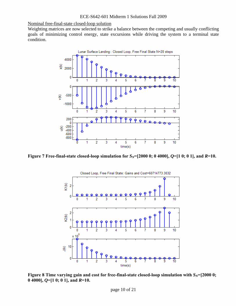
Nominal free-final-state closed-loop solution Weighting matrices are now selected to strike a balance between the competing and usually conflicting goals of minimizing control energy, state excursions while driving the system to a terminal state condition.

Figure 7 Free-final-state closed-loop simulation for SN=[2000 0; 0 4000], Q=[1 0; 0 1], and R=10.

Figure 8 Time varying gain and cost for free-final-state closed-loop simulation with SN=[2000 0; 0 4000], Q=[1 0; 0 1], and R=10.


page 11 of 21

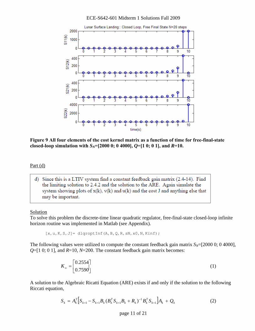
Figure 9 All four elements of the cost kernel matrix as a function of time for free-final-state closed-loop simulation with SN=[2000 0; 0 4000], Q=[1 0; 0 1], and R=10. Part (d)

Solution To solve this problem the discrete-time linear quadratic regulator, free-final-state closed-loop infinite horizon routine was implemented in Matlab (see Appendix).

[x,u,K,S,J]= dlqroptInf(A,B,Q,R,sN,x0,N,Kinf); The following values were utilized to compute the constant feedback gain matrix SN=[2000 0; 0 4000], Q=[1 0; 0 1], and R=10, N=200. The constant feedback gain matrix becomes:

⎥⎦

⎤⎢⎣

⎡=∞ 7590.0

2554.0K (1)

A solution to the Algebraic Ricatti Equation (ARE) exists if and only if the solution to the following Riccati equation,

[ ] kkkTkkkk

Tkkkk

Tkk QASBRBSBBSSAS ++−= +

−+++ 1

1111 )( (2)


page 12 of 21

converges to a finite solution. This equation was solved backwards in time, to yield

⎥⎦

⎤⎢⎣

⎡=∞ 7662.173443.6

3443.69431.5S (3)

Since the cost kernel matrix converges, a solution to the following ARE exists,

ASBRSBBSBSAS TTT ])([ 1−+−= (4) Using the Matlab dare() program to solve the ARE agreement is shown between the ARE and the time varying solution (3) for the cost kernel.

(5) Suboptimal Solution to the nominal free-final-state closed-loop solution in part (c)

Figure 10 Suboptimal control for free-final-state closed-loop solution simulation with SN=[2000 0; 0 4000], Q=[1 0; 0 1], and R=10 shows similar results to part (c).

[X,L,G] = dare(A,B,Q,R); X = 5.9431 6.3443 6.3443 17.7662


page 13 of 21

Figure 11 Suboptimal fixed gains and cost for free-final-state closed-loop simulation with SN=[2000 0; 0 4000], Q=[1 0; 0 1], and R=10 shows results similar to part (c). The cost is slightly less, 60.65e6, versus 60.7e6 from part (c).

Figure 12 All four elements of the cost kernel matrix as a function of time for the suboptimal free-final-state closed-loop simulation with SN=[2000 0; 0 4000], Q=[1 0; 0 1], and R=10.


page 14 of 21

Discussion Methods (b), (c), and (d) all strive to minimize the cost function or performance index over the time interval i to N defined by

( )∑−

=

++=1

, 21

21 N

ikkk

Tkkk

TkNN

TNNi uRuxQxxSxJ (1)

where, SN is a terminal condition weighting matrix, and Qk and Rk are time varying state and control weighting matrices respectively. Values for the weighting matrices are chosen by the design engineer to give the system a desired performance. For the fixed-final-state open-poop control implemented in part (b) the cost function reduces (for scalar u) to

( ) ...)(21

21 2

33222

211

1

+++== ∑−

=

uRuRuRuRuJN

ikkk

Tk (2)

Or, for constant weighting matrix, R,

...)(21 2

322

21 +++= uuuRJ (3)

As shown in part (a), the least squares solution, minimizes the square of the Euclidean, or 2-norm of the control energy,

( ) ( )...... 23

22

21

223

22

21

2 +++=+++= uuuuuuU (4) If we assume the control weighting matrix, Rk does not vary with time, then (2) and (4) only differ by a scale factor and will have the same solution for the minimum cost. Thus, it should be anticipated that the least squares method and the fixed-final-state open-loop control methods are equivalent and the implementations of the open-loop control methods will yield the same results only if R does not vary with time. For the free-final-state closed-loop control method algorithm of method (c) SN is usually non-zero to drive the system to xN , the terminal condition, and Qk is also usually non zero to penalize excessive state excursions. Also, as shown by simulation, by as SN and R become large (with Q set to zero), the results will approximate those of (a) and (b), since the terminal condition and the control energy expended are heavily weighted. But, the free-final-state method has the substantial benefit in that it is closed-loop, and will therefore will be more robust in that it will be more tolerant of un-modeled dynamics or disturbances.

The free-final-state closed-loop control method is complicated by the fact that off-line computations must be done to compute and store the optimal, time-varying gain, Kk, for use in the closed-loop system implementation. A simplification made in method (d) is to utilize a constant feedback gain, as N goes to infinity (infinite horizon). This is referred to as a sub-optimal feedback. However a performance penalty will be realized for this implementation and the designer must determine if the system performance is suitable for the application at hand.


page 15 of 21

The simulation results are summarized in the table below. As expected the least squares and fixed-final-state open-loop results are identical! As expected the free-final-state closed-loop results do not hit the terminal conditions exactly, as there are residual terminal velocity and position errors. Also note the fact that the open-loop methods effectively have no state weighting, Qk, so the states can be large as terminal conditions are approached (note average acceleration is shown in table). But of course method free-final-state method uses more fuel. Since one is typically concerned with having a smooth landing, or minimizing certain states such acceleration, jerk w, the impact of time-varying state weighting gain Qk and penalize state excursions more heavily as terminal conditions are approached to further optimize the trajectory should be investigated. The table also shows the performance penalty realized for the simplicity of the sub-optimal control approach, in that the final velocity is excessive. Clearly this would make for a rough landing and would not be suitable for implementation as it stands.

Method Final

Position (f)

Final Velocity

(fps)

Final Acceleration

(fps^2)

Cost (Fuel)

Total Cost

Robust

Least Squares Open Loop

0.0 0.0 -192.8 100188 100188 No

Fixed Final State Open Loop

0.0 0.0 -192.8 100188 100188 No

Free Final State Closed Loop

-0.500 .273 42.1 823980 60714773 Yes

Suboptimal Control Closed Loop

-92.0 31.8 -5.21 812570 60654939 Yes


page 16 of 21

Appendix Code Listing for part (a): clear all close all %************** %*** PART A *** %************** T=0.5; % Sample Time x0= 5000; % f v0=-500; %fps A = [1 T; 0 1] B = [T^2/2;T] %Drive the system to the origin in 20 steps N=20 %Terminal condition x0=[x0; v0] x20=[0; 0] CT=B; for i=1:N-1 CT = [CT A^i *B]; end P_INV=CT'*inv(CT*CT') u=(P_INV*(x20-A^N*x0)); u=flipud(u) %N Steps x = x0; traj = x0; for i=1:N xnext = A*x + B*u(i); traj = [traj xnext]; x = xnext; J(i)= 1/2 * u(i)^2; end traj u' h = figure; subplot(3,1,1) stem([0:N]*T,traj(1,:),'linewidth',2.0); ylabel('x(k)'); title(['Non Optimal N=20']); axis([-1*T T*(N+1) 0 5001]) title('Lunar Surface Landing:: Open Loop Least Squares Solution, N=20 steps')

subplot(3,1,2) stem([0:N]*T,traj(2,:),'linewidth',2.0); ylabel('v(k)');axis([-1*T,T*(N+1),-inf,inf]) subplot(3,1,3) stem([0:N-1]*T,u,'linewidth',2.0); ylabel('u(k)'); xlabel('time(s)'); axis([-1*T,T*(N+1),-inf,inf]) figure stem([0:N-1]*T,J,'linewidth',2.0); ylabel('J(k)'); xlabel('time(s)'); axis([-1*T,T*(N+1),-inf,inf]) title(['Cost as a Function of time:: Total cost=' sprintf('%7.0f',sum(J))])


page 17 of 21

Code Listing for part (b): clear all close all %************** %*** PART B *** %************** % Fixed Final State, Open Loop Control clear all N=20 R=1 T=0.5; % Sample TIme x0= 5000; % f v0=-500; %fps A = [1 T; 0 1] B = [T^2/2;T] %Drive the system to the origin in 20 steps N=20 %Terminal condition x0=[x0; v0] x20=[0; 0] rN=x20 G = zeros(2,2); %Compute Controllability Grammian for i=0:N-1 G=G + A^(N-i-1) * B * inv(R) * B' * (A')^(N-i-1); end Ginv = inv(G) %N Steps x = x0; traj = x0; for i=0:N-1 u(i+1) = inv(R) * B' * (A')^(N-i-1) * Ginv * (rN - A^N*x0) xnext = A*x + B*u(i+1); traj = [traj xnext]; x = xnext; J(i+1)= R/2 * u(i+1)^2; end traj u' h = figure; subplot(3,1,1) stem([0:N]*T,traj(1,:),'linewidth',2.0); ylabel('x(k)'); title(['Non Optimal N=20']);axis([-1,N+1,-inf,inf]) axis([-1*T T*(N+1) 0 5001]) title('Lunar Surface Landing::Fixed Final State, Open Loop Control, N=20 steps') subplot(3,1,2) stem([0:N]*T,traj(2,:),'linewidth',2.0); ylabel('v(k)');axis([-1*T,T*(N+1),-inf,inf]) subplot(3,1,3) stem([0:N-1]*T,u,'linewidth',2.0); ylabel('u(k)'); xlabel('k'); axis([-1*T,T*(N+1),-inf,inf]) figure stem([0:N-1]*T,J,'linewidth',2.0); ylabel('J(k)'); xlabel('k'); axis([-1*T,T*(N+1),-inf,inf]) title(['Cost as a Function of time:: Total cost=' sprintf('%7.0f',sum(J))]) sum(J)


page 18 of 21

Code Listing for part (c): clear all close all %************** %*** PART C *** %************** clear all T=0.5; % Sample TIme x0= 5000; % f v0=-500; %fps A = [1 T; 0 1] B = [T^2/2;T] %Drive the system to the origin in 20 steps N=20 %Terminal condition x0=[x0; v0] x20=[0; 0] rN=x20 Q=[1 0; 0 1]; R=10; sN=[2000 0; 0 4000]; [x,u,K,S,J]= dlqropt(A,B,Q,R,sN,x0,N); h = figure; subplot(3,1,1) stem([0:N]*T,x(1,:),'linewidth',2.0); ylabel('x(k)'); title(['Non Optimal N=20']);axis([-1*T,T*(N+1),-inf,inf]) title('Lunar Surface Landing:: Closed Loop, Free Final State N=20 steps') subplot(3,1,2) stem([0:N]*T,x(2,:),'linewidth',2.0); ylabel('v(k)');axis([-1*T,T*(N+1),-inf,inf]) subplot(3,1,3) stem([0:N-1]*T,u,'linewidth',2.0); ylabel('u(k)'); xlabel('time(s)'); axis([-1*T,T*(N+1),-inf,inf]) h = figure; subplot(3,1,1) stem([0:N-1]*T,K(:,1),'linewidth',2.0); ylabel('K1(k)');axis([-1*T,T*(N+1),-inf,1.1*max(K(:,1))]) title(['Closed Loop, Free Final State: Gains and Cost=' num2str(sum(J))]) subplot(3,1,2) stem([0:N-1]*T,K(:,2),'linewidth',2.0); ylabel('K2(k)');axis([-1*T,T*(N+1),-inf,inf]) subplot(3,1,3) stem([0:N]*T,J,'linewidth',2.0); ylabel('J(k)');axis([-1*T,T*(N+1),-inf,inf]);xlabel('time(s)'); h= figure subplot(4,1,1) stem([0:N]*T,S(:,1,1),'linewidth',2.0); ylabel('S11(k)');axis([-1*T,T*(N+1),-inf,inf]) title('Lunar Surface Landing:: Closed Loop, Free Final State N=20 steps') subplot(4,1,2) stem([0:N]*T,S(:,1,2),'linewidth',2.0); ylabel('S12(k)');axis([-1*T,T*(N+1),-inf,inf]) subplot(4,1,3) stem([0:N]*T,S(:,2,1),'linewidth',2.0); ylabel('S21(k)');axis([-1*T,T*(N+1),-inf,inf]) subplot(4,1,4) stem([0:N]*T,S(:,2,2),'linewidth',2.0); ylabel('S22(k)');axis([-1*T,T*(N+1),-inf,inf]);xlabel('time(s)'); K sum(u.^2)/2 sum(J)


page 19 of 21

function [x,u,K,S,J]=dlqropt(A,B,Q,R,s,x0,N) % Program to Cumpute and Simplate Optimal Feedback Control %Compute and Store Optimal Feedback Sequence n=length(A); S=zeros(N,n,n); K=zeros(N,n); S(N+1,:,:)=s; for k=N:-1:1 K(k,:)=inv(B'*s*B+R)*(B'*s*A); s=A' *(s-s*B*inv(B'*s*B+R)*B'*s) * A + Q; % Q+(R*s*a^2)/(r+s*b^2); S(k,:,:)=s; end %Apply Optimal Control to Plant (Forward Iteration) x=zeros(n,N); x(:,1)=x0; for k=1:N %Update Optimal Control Input u(k)=-K(k,:)*x(:,k); %Update Plant State J(k) = 0.5 * (x(:,k)'*Q*x(:,k) + u(k)'*R*u(k)); x(:,k+1)=A*x(:,k)+B*u(k); end J(N+1)=0.5*x(:,k)'*s*x(:,k);


page 20 of 21

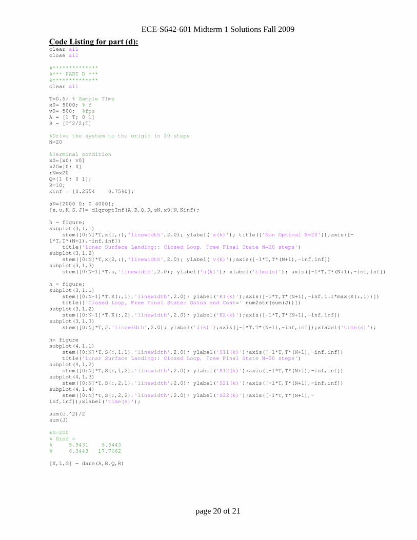
Code Listing for part (d): clear all close all %************** %*** PART D *** %************** clear all T=0.5; % Sample TIme x0= 5000; % f v0=-500; %fps A = [1 T; 0 1] B = [T^2/2;T] %Drive the system to the origin in 20 steps N=20 %Terminal condition x0=[x0; v0] x20=[0; 0] rN=x20 Q=[1 0; 0 1]; R=10; Kinf = [0.2554 0.7590]; sN=[2000 0; 0 4000]; [x,u,K,S,J]= dlqroptInf(A,B,Q,R,sN,x0,N,Kinf); h = figure; subplot(3,1,1) stem([0:N]*T,x(1,:),'linewidth',2.0); ylabel('x(k)'); title(['Non Optimal N=20']);axis([-1*T,T*(N+1),-inf,inf]) title('Lunar Surface Landing:: Closed Loop, Free Final State N=20 steps') subplot(3,1,2) stem([0:N]*T,x(2,:),'linewidth',2.0); ylabel('v(k)');axis([-1*T,T*(N+1),-inf,inf]) subplot(3,1,3) stem([0:N-1]*T,u,'linewidth',2.0); ylabel('u(k)'); xlabel('time(s)'); axis([-1*T,T*(N+1),-inf,inf]) h = figure; subplot(3,1,1) stem([0:N-1]*T,K(:,1),'linewidth',2.0); ylabel('K1(k)');axis([-1*T,T*(N+1),-inf,1.1*max(K(:,1))]) title(['Closed Loop, Free Final State: Gains and Cost=' num2str(sum(J))]) subplot(3,1,2) stem([0:N-1]*T,K(:,2),'linewidth',2.0); ylabel('K2(k)');axis([-1*T,T*(N+1),-inf,inf]) subplot(3,1,3) stem([0:N]*T,J,'linewidth',2.0); ylabel('J(k)');axis([-1*T,T*(N+1),-inf,inf]);xlabel('time(s)'); h= figure subplot(4,1,1) stem([0:N]*T,S(:,1,1),'linewidth',2.0); ylabel('S11(k)');axis([-1*T,T*(N+1),-inf,inf]) title('Lunar Surface Landing:: Closed Loop, Free Final State N=20 steps') subplot(4,1,2) stem([0:N]*T,S(:,1,2),'linewidth',2.0); ylabel('S12(k)');axis([-1*T,T*(N+1),-inf,inf]) subplot(4,1,3) stem([0:N]*T,S(:,2,1),'linewidth',2.0); ylabel('S21(k)');axis([-1*T,T*(N+1),-inf,inf]) subplot(4,1,4) stem([0:N]*T,S(:,2,2),'linewidth',2.0); ylabel('S22(k)');axis([-1*T,T*(N+1),-inf,inf]);xlabel('time(s)'); sum(u.^2)/2 sum(J) %N=200 % Sinf = % 5.9431 6.3443 % 6.3443 17.7662 [X,L,G] = dare(A,B,Q,R)


page 21 of 21

function [x,u,K,S,J]=dlqroptinf(A,B,Q,R,s,x0,N,Kinf) % Program to Cumpute and Simplate Optimal Feedback Control %Compute and Store Optimal Feedback Sequence n=length(A); S=zeros(N,n,n); K=zeros(N,n); S(N+1,:,:)=s; for k=N:-1:1 K(k,:)=Kinf; s=A' *(s-s*B*inv(B'*s*B+R)*B'*s) * A + Q; S(k,:,:)=s; end %Apply Optimal Control to Plant (Forward Iteration) x=zeros(n,N); x(:,1)=x0; for k=1:N %Update Optimal Control Input u(k)=-K(k,:)*x(:,k); %Update Plant State J(k) = 0.5 * (x(:,k)'*Q*x(:,k) + u(k)'*R*u(k)); x(:,k+1)=A*x(:,k)+B*u(k); end J(N+1)=0.5*x(:,k)'*s*x(:,k);

Optimal Control Simulation Problem -...

Documents

Transcript of Optimal Control Simulation Problem -...