Nonlinear Analysis: Real World Applications 12 (2011) 3452–3467

Contents lists available at SciVerse ScienceDirect

Nonlinear Analysis: Real World Applications

journal homepage: www.elsevier.com/locate/nonrwa

Optimal control of effort of a stage structured prey–predator fisherymodel with harvestingKunal Chakraborty a,∗, Sanjoy Das b, T.K. Kar ba Department of Mathematics, MCKV Institute of Engineering, 243 G.T. Road (N), Liluah, Howrah-711204, West Bengal, Indiab Department of Mathematics, Bengal Engineering and Science University, Shibpur, Howrah-711103, West Bengal, India

a r t i c l e i n f o

Article history:Received 4 February 2011Accepted 3 June 2011

Keywords:Prey–predator fisheryStage structureDifferential–algebraic systemSingularity induced bifurcationOptimal control

a b s t r a c t

This paper describes a prey–predator fisherymodel with stage structure for prey. The adultprey andpredator populations are harvested in the proposed system. Thedynamic behaviorof the model system is discussed. It is observed that singularity induced bifurcationphenomenon is appeared when variation of the economic interest of harvesting is takeninto account.We have incorporated state feedback controller to stabilize themodel systemin the case of positive economic interest. Fishing effort used to harvest the adult prey andpredator populations is used as a control to develop a dynamic framework to investigate theoptimal utilization of the resource, sustainability properties of the stock and the resourcerent earned from the resource. Pontryagin’s maximum principle is used to characterizethe optimal control. The optimal system is derived and then solved numerically using aniterativemethodwith Runge–Kutta fourth-order scheme. Simulation results show that theoptimal control scheme can achieve sustainable ecosystem.

© 2011 Elsevier Ltd. All rights reserved.

1. Introduction

Fisheries are systems that involve biological, economic and social/behavioral components. Each of these provides adistinctive perspective on the fishery, its goals, purpose and outputs. Biology and economics combine to produce outputs ofthe fishery,which are then comparedwith our expectations of the outputs.When the expectations andoutputs donotmatch,we use the process of regulation, which may act on any of the biological, economic and social components. According to theFood and Agriculture Organization of the United Nations [1], in the year 2005, about 50% of the fish stock under observationhas experienced overexploitation or depletion. These statistics reiterate the fact that fisheries need to be managed with aneffective and carefully defined objective in order to prevent overfishing and to allow the depleted stock to replenish. Again,economy is one of the conditioning factors of fishing activity. It is not necessary for the resource to exist biologically, butthere is an obvious economic interest in exploiting it. Economic analysis of the exploitation of natural resources applied tothe fisheries is a relatively recent branch of economics. This specialty is known as bioeconomics, and has developed sincethe end of the 1950s from the works of Gordon [2] and Schaefer [3].

There is a growing interest in using bioeconomic models as a tool for policy analysis to better understand the pathwaysof development and to assess the impact of alternative policies on the natural resource base and human welfare. One of thepotential benefits of these models is that one can get a better and more comprehensive indication of the feedback effectsbetween human activity and natural resources. The fundamental challenge of fisheries management is to take into accountboth the conservation of the resource base aswell as the exploitation of it by the industry (extractive and processing sectors).

∗ Corresponding author.E-mail addresses: kc_mckv@yahoo.co.in (K. Chakraborty), tkar1117@gmail.com (T.K. Kar).

1468-1218/$ – see front matter© 2011 Elsevier Ltd. All rights reserved.doi:10.1016/j.nonrwa.2011.06.007

K. Chakraborty et al. / Nonlinear Analysis: Real World Applications 12 (2011) 3452–3467 3453

Therefore, it is possible to make models that are theoretically more consistent and empirically more accurate. It is knownfrom the Poincare–Bendixson theory that two-dimensional continuous time models can approach either an equilibriumstate or a limit cycle but these models excluded chaotic behavior of the prey–predator systems, while three- and higher-dimensional models can exhibit more complex behavior. In this regard, staged models may provide in some situations aricher dynamics which leads to a better understanding of the interactions within the biological system under consideration.Such models may also incorporate parameters, such as different death rates for mature and immature species and variouseffects of intra-specific competition of species, which are biologically more meaningful.

It is globally accepted that random fishing of all fishes is not advisable for the persistence of the fishery. Matsuda andNishimori [4] analyzed that the exploitation of a population should be the mature population, which is not only moreappropriate toward the commercial purpose of the fishery but also restore the sustainable ecosystem. Again, biologicalviews of renewable resources management have been studied through harvesting models by many authors like Kar andChaudhuri [5,6], Ragozin and Brown [7], Mesterton-Gibbons [8], and Leung [9]. A significant volume of research like Kar andPahari [10], Magnusson [11], Wang et al. [12], Gao et al. [13], Arino et al. [14], Cao et al. [15], Bosch and Gabriel [16] etc. hasbeen carried out based on different kinds of predator–prey systemwith the division of predators into immature andmatureindividuals. But a few number of articles incorporated prey–predator models with stage structure of the prey species. Inthis paper, we investigate the dynamical behavior of the model system through incorporating the stage structure of preyspecies.

For the purpose of system modeling and analysis in different fields of applied sciences and engineering, differential–algebraic equations (DAEs) are considered as an essential tool. Naturally, differential or algebraic equations usually form themathematical model of the system. It is observed that a numerous number of research articles proposed the populationdynamics and analyzed the stability of the system in the presence of harvesting effort and time delay but quite a fewnumber of articles investigated the dynamical behavior of bioeconomic models using DAEs. Kar and Chakraborty [17]proposed a biological economic model based on the prey–predator dynamics and found singularity induced bifurcation(SIB) phenomenon and impulsive behavior of the model system at the interior equilibrium point using DAEs. They havedesigned an optimal controller to eliminate singularity induced bifurcation and impulsive behavior of the model systemwhen positive economic interest is taken into account.

The books of Clark [18,19] andMark Kot [20] are extremely relevant to the optimal control problems. Jerry and Rassi [21]examined a structured fishing model, basically displaying the two stages of ages of a fish population, which are in our casejuveniles and adults. They associated the maximization of the total discounted net revenues derived by the exploitation ofthe stock to thismodel. They also developed the exploitation strategy of the optimal control problem. Ding et al. [22] studiedthe control problem of maximizing the net benefit in the conservation of a single species with a fixed amount of resources.They investigated the existence of an optimal control and the uniqueness and characterization of the optimal control.

Here,we consider a simple harvested prey–predatormodelwith stage structure for preywhich is to be used to investigatethe comparative study of the resource stock and harvesting. The existence of SIB phenomenon is verified at the interiorequilibrium of the model system with zero economic profit and state feedback controller is designed to overcome SIB.The control problem is formulated and the corresponding optimality system that characterizes the (continuous) optimalcontrol solution is described. We find a characterization for the optimal control and show numerical results for scenarios ofdifferent illustrative parameter sets. The numerical results providemore realistic features of themodel system. The solutionis performed using an iterative method with Runge–Kutta fourth-order scheme of optimal control.

2. Model description and assumptions

We consider a prey–predator model with stage structure for prey and it is assumed that only adult prey and predatorpopulations are harvested. Let us assume x, y and z are respectively the size of juveniles, adults prey population and predatorpopulation at time t . It is considered that all these populations are growing in closed homogeneous environment. At anytime t , the birth rate of the juvenile prey populations is assumed to be proportional to the density of existing adult preypopulation with proportionality constant r and the rate of transformation of the adult prey is proportional to the densityof existing juvenile prey with proportionality constant s. The predator population consumes the juvenile and adult preypopulations respectively at the rate α and β and contributes to its growth rate αxz and βyz. Keeping these aspects in view,the dynamics of the system may be governed by the following system of differential equations:

dxdt

= ry − d1x − sx − γ x2 − αxz, (1a)

dydt

= sx − d2y − λy2 − βyz − h1(t), (1b)

dzdt

= αxz + βyz − d3z − σ z2 − h2(t) (1c)

where d1(γ ), d2(λ) and d3(σ ) are respectively the death rates (intra-specific coefficients) of the juvenile prey, adult preyand predator populations. h1(t) and h2(t) are respectively the harvesting of adult prey and predator populations at time t .

3454 K. Chakraborty et al. / Nonlinear Analysis: Real World Applications 12 (2011) 3452–3467

If we consider the commercial purpose of the fishery, then it is necessary to harvest from the fishery but harvestingshould be regulated in such a way that the fishermen restrict themselves to harvest immature fishes since the immaturefishes have low commercial value compared to themature fishes. This type of harvesting is not only achieve the commercialpurpose of the fishery but also helpful for the conservation of the fishery. This can be made by adjusting the mesh size ofthe net so that when nets are placed in water, they can capture all the fish except those that are small enough to swimthrough the mesh. The functional form of the harvest is generally considered using the phrase catch-per-unit-effort (CPUE)hypothesis [19] to describe an assumption that catch per unit effort is proportional to the stock level. Therefore, harvestingfunction h1(t) and h2(t) can be written as:

h1 = q1Ey, (2a)h2 = q2Ez, (2b)

where q1 and q2 are the catchability coefficients respectively for adult prey and predator populations, E is the effort used toharvest the populations. Let us extend our model by considering the following algebraic equation:

(p1q1y + p2q2z − c)E − m = 0, (3)

where c is the constant fishing cost per unit effort, p1 and p2 are the constant price per unit biomass of landed fish respectivelyfor adult prey and predator populations andm is the total economic rent obtained from the fishery.

Hence, using (2) system (1) finally becomes

dxdt

= ry − d1x − sx − γ x2 − αxz, (4a)

dydt

= sx − d2y − λy2 − βyz − q1Ey, (4b)

dzdt

= αxz + βyz − d3z − σ z2 − q2Ez, (4c)

(p1q1y + p2q2z − c)E − m = 0, (4d)

with initial conditions x(0) ≥ 0, y(0) ≥ 0 and z(0) ≥ 0.

3. Qualitative analysis of model system

In this section, we mainly investigate the occurrence of singularity induced bifurcation and the effects of economicprofit on the dynamics of the system (4). From the view of ecological management, it is sufficient to consider the interiorequilibrium point of the system (4) since the biological interpretation of the interior equilibrium implies that juvenile prey,adult prey and predator populations exist for finite fishing effort. Let P∗(x∗, y∗, z∗, E∗) be the interior equilibrium of thesystem (4).

The differential–algebraic system (4) can be expressed in the following way:

f (X, E,m) =

f1(X, E,m)f2(X, E,m)f3(X, E,m)

=

ry − d1x − sx − γ x2 − αxzsx − d2y − λy2 − βyz − q1Ey

αxz + βyz − d3z − σ z2 − q2Ez

,

g(X, E,m) = (p1q1y + p2q2z − c)E − m,

where X = (x, y, z)t .Let us now study the dynamic behavior of the system (4). The local stability of the interior equilibrium point,

P∗(x∗, y∗, z∗, E∗) can be investigated using the SIB phenomena based on the assumption that the interior equilibrium pointexists. From system (4), we have the following matrix:

M = DX f − DE f (DEg)−1DXg

=

−

ry∗

x− γ x r −αx

s −sxy∗

− λy∗+

p1q21y∗E∗

p1q1y∗ + p2q2z∗ − c−βy∗

+p2q1q2y∗E∗

p1q1y∗ + p2q2z∗ − c

αz∗ βz∗+

p1q1q2z∗E∗

p1q1y∗ + p2q2z∗ − c−σ z∗

+p2q22z

∗E∗

p1q1y∗ + p2q2z∗ − c

.

To check the existence of the SIB phenomena, total economic rent m is assumed to be the bifurcation parameter.Consequently we have the following theorem:

Theorem 1. The differential–algebraic system (4) has a singularity induced bifurcation at the interior equilibrium pointP∗(x∗, y∗, z∗, E∗). When the bifurcation parameter m increases through zero, the stability of the interior equilibrium pointP∗(x∗, y∗, z∗, E∗) changes from stable to unstable.

K. Chakraborty et al. / Nonlinear Analysis: Real World Applications 12 (2011) 3452–3467 3455

Fig. 1. Variation of optimal prey and predator biomass and fishing effort with the increasing time. The solid line corresponds to r = 1.8, the dotted lineto r = 1.5 and the dashed line to r = 2.

Proof. It is evident that DEg = p1q1y + p2q2z − c has a simple zero eigenvalue. Let us now define

∆(X, E,m) = DEg = p1q1y + p2q2z − c.

(i) From the existence of P∗(x∗, y∗, z∗, E∗) it follows that

Trace[DE f adj(DEg)DXg]P∗ = −p1q21y∗E∗

− p2q22z∗E∗

= 0.

(ii) It can be proved that

DX f DE fDXg DEg

P∗

=

−

ryx

− γ x r −αx 0

s −sxy

− λy −βy −q1y

αz βz −σ z −q2z0 p1q1E p2q2E 0

P∗

=1

x∗y∗E∗z∗

[y∗p1q1{y∗(ry∗σ + x∗2(α2+ γ σ))q1 − (sx∗2α + y∗β(ry∗

+ x∗2γ ))q2} + p2q2{y∗2(rx∗α + ry∗β + x∗2βγ )q1 + (sx∗3γ + y∗2(ry∗+ x∗2γ )λ)q2}] = 0,

(iii) It can also be shown that

DX f DE f DmfDXg DEg DmgDX∆ DE∆ Dm∆

P∗

=

−ryx

− γ x r −αx 0 0

s −sxy

− λy −βy −q1y 0

αz βz −σ z −q2z 00 p1q1E p2q2E 0 −10 p1q1 p2q2 0 0

P∗

3456 K. Chakraborty et al. / Nonlinear Analysis: Real World Applications 12 (2011) 3452–3467

Fig. 2. Variation of optimal prey and predator biomass and fishing effort with the increasing time. The solid line corresponds to s = 1.5, the dotted line tos = 1.3 and the dashed line to s = 1.4.

=1

x∗y∗z∗

[y∗p1q1{y∗(ry∗σ + x∗2(α2+ γ σ))q1 − (sx∗2α + y∗β(ry∗

+ x∗2γ ))q2} + p2q2{y∗2(rx∗α + ry∗β + x∗2βγ )q1 + (sx∗3γ + y∗2(ry∗

+ x∗2γ )λ)q2}] = 0.

It is noted that conditions (ii) and (iii) exist if ry∗

sx∗ >p1p2.

It is observed from (i)–(iii) that all the conditions for singularity induced bifurcation are satisfied (see [23]). Hence thedifferential–algebraic system (4) has a singularity induced bifurcation at the interior equilibrium point P∗(x∗, y∗, z∗, E∗) atthe bifurcation valuem = 0.

Again, it is noted that

M1 = −Trace[DE f adj(DEg)DXg]P∗ = p1q21y∗E∗

+ p2q22z∗E∗

= 0.

M2 =

Dλ∆ −

DX∆ DE∆

DX f DE fDXg DEg

−1 DλfDλg

P∗

=1E∗

.

Therefore, the existence of interior equilibrium point implies that

M1

M2= (p1q21y

∗+ p2q22z

∗)E∗2 > 0.

Hence, it can be concluded that when m increases through zero, one eigenvalue of the model system (4) moves from C− toC+ along the real axis by diverging through ∞ (see [23]). Consequently, the stability of the model system (4) is influencedthrough this behavior i.e., the stability of the system at the interior equilibrium point P∗(x∗, y∗, z∗, E∗) changes from stableto unstable. �

In consequence to the above theorem, it is clear that the differential–algebraic model system (4) becomes unstable whenthe economic interest of the harvesting is considered to be positive. If we consider the economic perspective of the fishery,

K. Chakraborty et al. / Nonlinear Analysis: Real World Applications 12 (2011) 3452–3467 3457

Fig. 3. Variation of optimal prey and predator biomass and fishing effort with the increasing time. The solid line corresponds to α = 0.5, the dotted lineto α = 0.6 and the dashed line to α = 0.7.

it is obvious that fishery agencies are interested toward the positive economic rent earned from the fishery. It is also notedthat an impulsive phenomenon can occur through singularity induced bifurcation in prey–predator ecosystem which maylead to the collapse of the sustainable ecosystem of the prey–predator fishery.

Therefore, it is necessary to reduce the impulsive phenomenon from the prey–predator ecosystem to resume thesustainability of the ecosystem and stabilize the model system when economic interest of the fishery is considered to bepositive.

Thus, to stabilize the model system (5) in the case of positive economic interest a state feedback controller [24] can bedesigned of the form w(t) = u(E(t) − E∗), where u stands for net feedback gain.

After introducing the state feedback controller, we rewrite the system (4) as:

dxdt

= ry − d1x − sx − γ x2 − αxz, (5a)

dydt

= sx − d2y − λy2 − βyz − q1E1y, (5b)

dzdt

= αxz + βyz − d3z − σ z2 − q2E2z, (5c)

(p1q1y + p2q2z − c)E − m + u(E(t) − E∗) = 0. (5d)

Consequently, we have the following theorem:

Theorem 2. The differential–algebraic system (5) is stable at the interior equilibrium point, P∗(x∗, y∗, z∗, E∗), of the system (4) ifu > max

a1b1

,a2b2

,a3b3

where

a1 = E∗(y∗p1q21 + z∗p2q22),

b1 =sx∗

y∗+

ry∗

x∗+ x∗γ + y∗λ + z∗σ ,

3458 K. Chakraborty et al. / Nonlinear Analysis: Real World Applications 12 (2011) 3452–3467

Fig. 4. Variation of optimal prey and predator biomass and fishing effort with the increasing time. The solid line corresponds to β = 0.8, the dotted lineto β = 0.6 and the dashed line to β = 1.

a2 = E∗(y∗2(ry∗+ x∗(x∗γ + z∗σ))p1q21 + x∗y∗2z∗β(−p1 + p2)q1q2 + z∗(sx∗2

+ y∗(ry∗+ x∗(x∗γ + y∗λ)))p2q22),

b2 = sx∗3γ + ry∗2(y∗λ + z∗σ) + x∗y∗2z∗(β2+ λσ) + x∗2(y∗2γ λ + sz∗σ + y∗z∗(α2

+ γ σ)),

a3 = E∗(y∗p1q1(y∗(ry∗σ + x∗2(α2+ γ σ))q1 − (ry∗2β + x∗2(sα + y∗βγ ))q2) + p2q2(y∗2(rx∗α

+ ry∗β + x∗2βγ )q1 + (sx∗3γ + y∗2(ry∗+ x∗2γ )λ)q2)),

b3 = sx∗2(y∗αβ + x∗(α2+ γ σ)) + y∗2(r(x∗αβ + y∗β2

+ y∗λσ) + x∗2(β2γ + α2λ + γ λσ)).

Proof. For the system (5), we can obtain the following Jacobian at the interior equilibrium point P∗(x∗, y∗, z∗, E∗), of thesystem (4),

N =

−

ry∗

x∗− γ x∗ r −αx∗

s −sx∗

y∗− λy∗

+p1q21y

∗E∗

u−βy∗

+p2q1q2y∗E∗

u

αz∗ βz∗+

p1q1q2z∗E∗

u−σ z∗

+p2q22z

∗E∗

u

.

Therefore, the characteristic polynomial of the matrix N is given by

µ3+ w1(X, E)µ2

+ w2(X, E)µ + w3(X, E) = 0,

where

w1 =sx∗

y∗+

ry∗

x∗+ x∗γ + y∗λ + z∗σ −

E∗y∗p1q21u

−E∗z∗p2q22

u,

K. Chakraborty et al. / Nonlinear Analysis: Real World Applications 12 (2011) 3452–3467 3459

Fig. 5. Variation of optimal prey and predator biomass and fishing effort with the increasing time. The solid line corresponds to γ = 0.2, the dotted lineto γ = 0.02 and the dashed line to γ = 2.

w2 = x∗z∗α2+ y∗z∗β2

+sx∗2γ

y∗+

ry∗2λ

x∗+ x∗y∗γ λ +

sx∗z∗σ

y∗+

ry∗z∗σ

x∗+ (x∗γ + y∗λ)z∗σ

−E∗ry∗2p1q21

ux∗−

E∗x∗y∗γ p1q21u

−E∗y∗z∗σp1q21

u+

E∗y∗z∗βp1q1q2u

−E∗y∗z∗βp2q1q2

u

−E∗sx∗z∗p2q22

uy∗−

E∗ry∗z∗p2q22ux∗

−E∗x∗z∗γ p2q22

u−

E∗y∗z∗λp2q22u

,

w3 =sx∗2z∗

y∗(α2

+ γ σ) + (sx∗+ ry∗)z∗αβ +

ry∗2z∗

x∗(β2

+ λσ) + x∗y∗z∗(β2γ + α2λ + γ λσ)

+E∗sx∗z∗αp1q1q2

u−

E∗x∗y∗z∗α2p1q21u

−E∗ry∗2z∗σp1q21

ux∗−

E∗x∗y∗z∗γ σp1q21u

+E∗ry∗2z∗βp1q1q2

ux∗+

E∗x∗y∗z∗βγ p1q1q2u

−E∗ry∗z∗αp2q1q2

u−

E∗x∗y∗z∗γ λp2q22u

−E∗ry∗2z∗βp2q1q2

ux∗−

E∗x∗y∗z∗βγ p2q1q2u

−E∗sx∗2z∗γ p2q22

uy∗−

E∗ry∗2z∗λp2q22ux∗

.

According to the Routh–Hurwitz criterion, it can be concluded that the system (5) is stable at the interior equilibrium pointP∗(x∗, y∗, z∗, E∗), of the system (4) if the net feedback gain u satisfies the following condition:

u > maxa1b1

,a2b2

,a3b3

where a1, a2, a3, b1, b2 and b3 are as given in the theorem.

Hence, it is possible to design a suitable controller function such that the singularity induced bifurcation can beeliminated. Thus, the impulsive phenomenon of a sustainable ecosystem can also be removed. Again, the economic interestof fishery managers may be achieved by using suitably designed state feedback controller. �

3460 K. Chakraborty et al. / Nonlinear Analysis: Real World Applications 12 (2011) 3452–3467

Fig. 6. Variation of optimal prey and predator biomass and fishing effort with the increasing time. The solid line corresponds to λ = 0.4, the dotted lineto λ = 0.1 and the dashed line to λ = 0.8.

4. The optimal control problem

In commercial exploitation of renewable resources the fundamental problem from the economic point of view, is todetermine the optimal trade-off between present and future harvests. The emphasis of this section is on the profit-makingaspect of fisheries. It is a thorough study of the optimal harvesting policy and the profit earned by harvesting, focusing onquadratic costs and conservation of fish population by constraining the latter to always stay above a critical threshold. Theprime reason for using quadratic costs is that it allows us to derive an analytical expression for the optimal harvest; theresulting solution is different from the bang–bang solution which is usually obtained in the case of a linear cost function.It is assumed that price is a function which decreases with increasing biomass. Thus, to maximize the total discounted netrevenues from the fishery, the optimal control problem can be formulated as:

J(E) =

∫ tf

t0e−δt

[(p1 − v1q1Ey)q1Ey + (p2 − v2q2Ez)q2Ez − cE]dt (6)

where v1 and v2 are the economic constants and δ is the instantaneous annual discount rate.The problem (6), subject to population equations (4a)–(4c) and control constraints 0 ≤ E ≤ Emax, can be solved by

applying Pontryagin’s maximum principle. The convexity of the objective function with respect to E, the linearity of thedifferential equations in the control and the compactness of the range values of the state variables can be combined to givethe existence of the optimal control.

Suppose Eδ is an optimal control with corresponding states xδ, yδ and zδ . We are seeking to derive optimal control Eδ suchthat

J(Eδ) = max{J(E) : E ∈ U},

where U is the control set defined by

U = {E : [t0, tf ] → [0, Emax] | E is Lebesgue measurable}.

K. Chakraborty et al. / Nonlinear Analysis: Real World Applications 12 (2011) 3452–3467 3461

Fig. 7. Variation of optimal prey and predator biomass and fishing effort with the increasing time. The solid line corresponds to σ = 0.6, the dotted lineto σ = 0.4 and the dashed line to σ = 0.8.

The Hamiltonian of this control problem is

H = [(p1 − v1q1Ey)q1Ey + (p2 − v2q2Ez)q2Ez − cE] + λ1(ry − d1x − sx − γ x2 − αxz)+ λ2(sx − d2y − λy2 − βyz − q1Ey) + λ3(αxz + βyz − d3z − σ z2 − q2Ez),

where λ1(t), λ2(t) and λ3(t) are the adjoint variables.The transversality conditions give λi(tf ) = 0, i = 1, 2, 3.Now, it is possible to find the characterization of the optimal control Eδ . On the set {t | 0 < Eδ(t) < Emax}, we have

∂H∂E

= y(−λ2 + p1)q1 + z(−λ3 + p2)q2 − 2Ey2q21v1 − 2Ez2q22v2 − c = 0 at Eδ(t).

This implies that,

Eδ =yδp1q1 + zδp2q2 − yδλ2q1 − zδλ3q2 − c

2(yδ2q21v1 + zδ2q22v2)

. (7)

Now, the adjoint equations are

dλ1

dt= δλ1 −

∂H∂x

= δλ1 − [(−d1 − s − zα − 2xγ )λ1 + sλ2 + zαλ3], (8)

dλ2

dt= δλ2 −

∂H∂y

= δλ2 − [rλ1 − d2λ2 − zβλ2 − 2yλλ2 + zβλ3 + E(−λ2 + p1)q1 − 2E2yq21v1], (9)

dλ3

dt= δλ3 −

∂H∂z

= δλ3 − [−xαλ1 − yβλ2 − d3λ3 + xαλ3 + yβλ3 − 2zλ3σ − Eλ3q2 + Ep2q2 − 2E2zq22v2]. (10)

Therefore, we summarize the above analysis by the following theorem:

Theorem 3. There exists an optimal control Eδ and corresponding solutions xδ, yδ and zδ thatmaximizes J(E) over U. Furthermore,there exists adjoint functions λ1, λ2 and λ3 satisfying the Eqs. (8)–(10) with transversality conditions λi(tf ) = 0, i = 1, 2, 3.Moreover, the optimal control is given by Eδ =

yδp1q1+zδp2q2−yδλ2q1−zδλ3q2−c2(yδ2q21v1+zδ2q22v2)

.

3462 K. Chakraborty et al. / Nonlinear Analysis: Real World Applications 12 (2011) 3452–3467

Fig. 8. Variation of optimal prey and predator biomass and fishing effort with the increasing time. The solid line corresponds to p1 = 1.0, the dotted lineto p1 = 1.5 and the dashed line to p1 = 2.0.

5. Numerical simulation of optimal control problem

The numerical simulation of optimal control [25] under various parameter sets can be done using fourth-orderRunge–Kutta forward–backward sweep method. In this method, the system state equations (4a)–(4c) and theircorresponding adjoint Eqs. (8)–(10) are simultaneously solved. Initially, we make a guess for optimal control and then solvethe system of state equations (4a)–(4c) forward in time using the Runge–Kutta method with the initial conditions x0, y0and z0. Then, using the state values, the adjoint Eqs. (8)–(10) are solved backward in time using the Runge–Kutta methodwith the transversality conditions. At this point, the optimal control is updated using the values for the state and adjointvariables. The updated control replaces the initial control and the process is repeated until the successive iterates of controlvalues are sufficiently close. The convergence of such an iterative method is based on the work of Hackbush [26].

At first, we discretize the interval [t0, tn] at the points ti = t0 + ih (i = 0, 1, 2, . . . , n) where h is the time step such thattn = tf . Now a combination of forward and backward difference approximation is considered to solve the system. The timederivative of the state variables can be expressed by their first-order forward difference as follows:

xi+1 − xih

= ryi − d1xi+1 − sxi+1 − γ x2i+1 − αxi+1zi,

yi+1 − yih

= sxi+1 − d2yi+1 − λy2i+1 − βyi+1zi − q1Eiyi+1,

zi+1 − zih

= αxi+1zi+1 + βyi+1zi+1 − d3zi+1 − σ z2i+1 − q2Eizi+1.

By using a similar technique, we approximate the time derivative of the adjoint variables by their first-order backwarddifference and we use the appropriate scheme as follows:

λ1n−i

− λ1n−i−1

h= δλ1

n−i−1− [(−d1 − s − zi+1α − 2xi+1γ )λ1

n−i−1+ sλ2

n−i+ zi+1αλ3

n−i],

λ2n−i

− λ2n−i−1

h= δλ2

n−i−1− [rλ1

n−i−1− d2λ2

n−i−1− zi+1βλ2

n−i−1− 2yi+1λλ2

n−i−1

+ zi+1βλ3n−i

+ Ei(−λ2n−i−1

+ p1)q1 − 2Ei2yi+1q21v1],

K. Chakraborty et al. / Nonlinear Analysis: Real World Applications 12 (2011) 3452–3467 3463

Fig. 9. Variation of optimal prey and predator biomass and fishing effort with the increasing time. The solid line corresponds to p2 = 1.5, the dotted lineto p2 = 1.0 and the dashed line to p2 = 2.0.

λ3n−i

− λ3n−i−1

h= δλ3

n−i−1− [−xi+1αλ1

n−i−1− yi+1βλ2

n−i−1− d3λ3

n−i−1+ xi+1αλ3

n−i−1

+ yi+1βλ3n−i−1

− 2zi+1λ3n−i−1σ − Eiλ3

n−i−1q2 + Eip2q2 − 2Ei2zi+1q22v2].

As the problem is not a case study, the real world data are not available for this model. We, therefore, take here somehypothetical data with the sole purpose of illustrating the results that we have established in the previous sections. Thefollowing parameters and initial values in appropriate units are used for the numerical simulations. We have analyzed theproposed system for a time span of 4 years. r = 1.8, d1 = 0.001, s = 1.5, α = 0.5, γ = 0.2, d2 = 0.002, λ = 0.4, β =

0.8, d3 = 0.005, σ = 0.6, x0 = 2.2, y0 = 2.5, z0 = 2.6, q1 = 0.8, q2 = 0.2, p1 = 1.0, p2 = 1.5, v1 = 1.75, v2 =

1.45, c = 0.05, δ = 0.01, tf = 4.The proportionality constant r of juvenile prey population has an important role on the dynamics of the system. It is

clearly observed from Fig. 1 that, in presence of harvesting, all the population decreases with increasing time but aftera particular time span the optimal control (fishing effort used to harvest) tends to zero when proportionality constantr increases. It is obvious that for the higher proportionality constant r the quantity of juvenile prey population shouldbe increased consequently the quantity of adult prey population also increased which is clearly shown in the figure.The interesting fact of the considered model system is that the predator population gets increased with the increasingproportionality constant r of juvenile prey population and the existence of the predator population is ensured due to thefact that the fishing effort decreases with the increasing proportionality constant r of juvenile prey population.

It is clear from Fig. 2 that the proportionality constant s of juvenile prey population and adult prey population has greatinfluence on the dynamics of the system. It is noted from the figure that for lower proportionality constant s, fishing effortused to harvest tends to zero consequently the quantity of prey as well as predator population get increased. However, itmay also be noted that initially all the population decreases with increasing time due to increasing fishing effort but aftera particular time span fishing effort used to harvest decreases and ultimately tends to zero consequently all the populationgetting increased. Thus the higher rate of conversion of juvenile prey population into adult prey population may collapsethe entire ecosystem. Hence, the optimal control (fishing effort) can be suitably designed so that the prey and predatorpopulations may get protection from extinction.

The impacts of predation on a prey–predator fishery model are illustrated in Figs. 3 and 4. According to the formation ofthe model, the predator population entirely dependent on the prey population and there is no alternative source of prey.

3464 K. Chakraborty et al. / Nonlinear Analysis: Real World Applications 12 (2011) 3452–3467

Fig. 10. Variation of optimal prey and predator biomass and fishing effort with the increasing time. The solid line corresponds to v1 = 1.75, the dottedline to v1 = 1.5 and the dashed line to v1 = 2.0.

Thus, for a higher rate of predation of juvenile prey population it is obvious that the predator population gets increasedbut due to the simultaneous harvesting effect of predator population juvenile prey population increases with increasingrate of predation. This effect is not permanent since it is clearly observed from Fig. 3 that finally juvenile as well as adultprey population decreases with increasing rate of predation. It is also observed that harvesting has a great impact on thepopulations. Since the catch rate exhibits solution effects with respect to both the stock and effort levels, it is interesting toobserve that the fishing effort gets decreased after a particular time span and ultimately tend to zero; as a result the quantityof prey as well as predator population increases. Hence, the fully dynamic interaction between the predation and fishingeffort plays an important role for the existence of the entire ecosystem.

The density dependent mortality rate of populations is an important factor in population dynamics toward a sustainableecosystem. Several researchers concluded that an impulsive phenomenon can occur due to the decreasing rate of densitydependent mortality rate of populations in a prey–predator ecosystem which may leads to the collapse of the sustainableecosystem of the fishery. It is evident from Figs. 5–7 that density dependentmortality rate of populations plays an importantrole in the case of internal interactions among the species. In the presence of harvesting it becomes a key factor for theexistence of the species of the ecosystem.

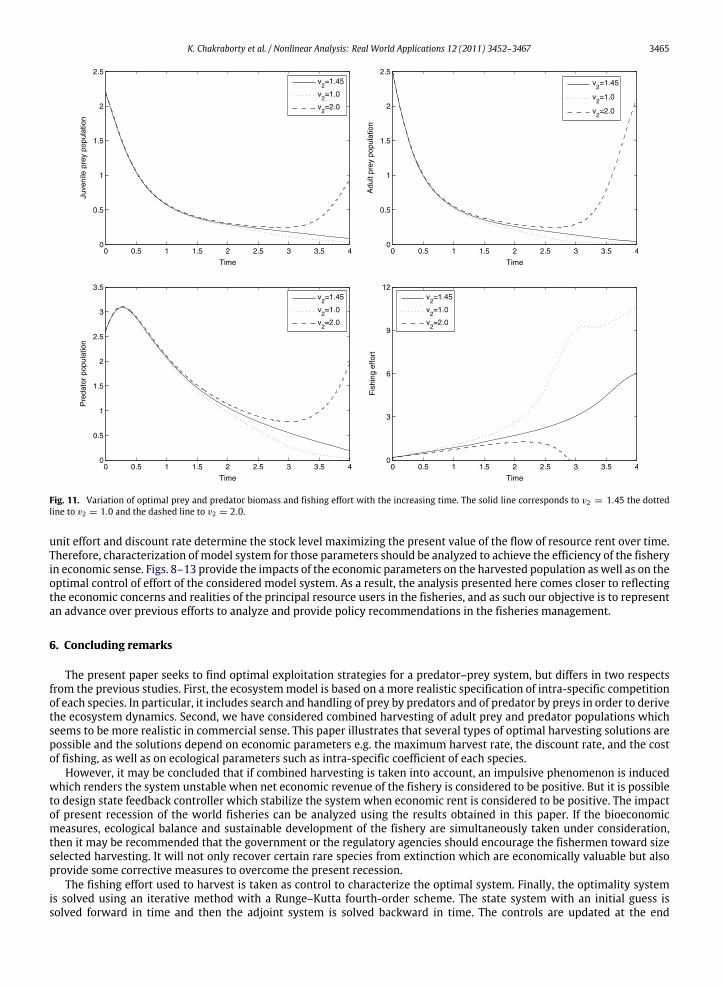
The impact of constant price per unit biomass of catch on the harvested population is described in the Figs. 8–11. It isnatural that the price per unit biomass of catch is inversely proportional to the harvested population. It is evident fromthe Figs. 8 and 9 that the harvested population decreases with the increasing price per unit biomass of catch. The pricefunction of the harvested population is formulated based on the inverse demandhypothesiswhich seems to bemore realisticpart of the paper and the Figs. 10 and 11 clearly indicate the results. However, the controllability of the fishing effort withthe price per unit biomass of catch is also necessary. It is noted that when price per unit biomass of catch decreases theconsequent population get increased though at the initial stage due to the effect of harvesting the population decreaseswith the increasing fishing effort. But with the increasing time, the optimal efforts correspond to the higher price per unitbiomass of catch increasesmore rapidly compared to the optimal efforts correspond to lower price per unit biomass of catchdue to the inverse demand function.

The inclusion of economic factors in fishery models is very important to assess the economic consequences of thefisheries. To attain efficiency in the economic sense, we need to take into account the costs of fishing and revenues thatwe get from selling the harvested fish. The economic parameters such as price per unit biomass of catch, fishing cost per

K. Chakraborty et al. / Nonlinear Analysis: Real World Applications 12 (2011) 3452–3467 3465

Fig. 11. Variation of optimal prey and predator biomass and fishing effort with the increasing time. The solid line corresponds to v2 = 1.45 the dottedline to v2 = 1.0 and the dashed line to v2 = 2.0.

unit effort and discount rate determine the stock level maximizing the present value of the flow of resource rent over time.Therefore, characterization of model system for those parameters should be analyzed to achieve the efficiency of the fisheryin economic sense. Figs. 8–13 provide the impacts of the economic parameters on the harvested population as well as on theoptimal control of effort of the considered model system. As a result, the analysis presented here comes closer to reflectingthe economic concerns and realities of the principal resource users in the fisheries, and as such our objective is to representan advance over previous efforts to analyze and provide policy recommendations in the fisheries management.

6. Concluding remarks

The present paper seeks to find optimal exploitation strategies for a predator–prey system, but differs in two respectsfrom the previous studies. First, the ecosystemmodel is based on a more realistic specification of intra-specific competitionof each species. In particular, it includes search and handling of prey by predators and of predator by preys in order to derivethe ecosystem dynamics. Second, we have considered combined harvesting of adult prey and predator populations whichseems to be more realistic in commercial sense. This paper illustrates that several types of optimal harvesting solutions arepossible and the solutions depend on economic parameters e.g. the maximum harvest rate, the discount rate, and the costof fishing, as well as on ecological parameters such as intra-specific coefficient of each species.

However, it may be concluded that if combined harvesting is taken into account, an impulsive phenomenon is inducedwhich renders the system unstable when net economic revenue of the fishery is considered to be positive. But it is possibleto design state feedback controller which stabilize the system when economic rent is considered to be positive. The impactof present recession of the world fisheries can be analyzed using the results obtained in this paper. If the bioeconomicmeasures, ecological balance and sustainable development of the fishery are simultaneously taken under consideration,then it may be recommended that the government or the regulatory agencies should encourage the fishermen toward sizeselected harvesting. It will not only recover certain rare species from extinction which are economically valuable but alsoprovide some corrective measures to overcome the present recession.

The fishing effort used to harvest is taken as control to characterize the optimal system. Finally, the optimality systemis solved using an iterative method with a Runge–Kutta fourth-order scheme. The state system with an initial guess issolved forward in time and then the adjoint system is solved backward in time. The controls are updated at the end

3466 K. Chakraborty et al. / Nonlinear Analysis: Real World Applications 12 (2011) 3452–3467

Fig. 12. Variation of optimal prey and predator biomass and fishing effort with the increasing time. The solid line corresponds to c = 0.05, the dotted lineto c = 0.03 and the dashed line to c = 0.08.

Fig. 13. Variation of optimal present value of the fishery with the increasing time. The solid line corresponds to δ = 0.01, the dotted line to δ = 0.03 andthe dashed line to δ = 0.05.

of each iteration using the formula for optimal controls. The iterations continue until convergence is achieved. Again, itis necessary to perform the numerical simulations to accumulate information about the variability of results from eachstrategy of a model system and summarization of the obtained results. We have discussed an efficient numerical methodbased on optimal control to identify the best management policies to overcome the exploitation of the fishery and achieve

K. Chakraborty et al. / Nonlinear Analysis: Real World Applications 12 (2011) 3452–3467 3467

optimality in economic sense. The present work describes the use of harvesting as a control to obtain strategies for thecontrol of a prey–predator system with stage structure. We find that it is possible to control the system in such a way thatthe system approaches a required state, using the harvesting as the control. The considered model system incorporates afully dynamic interaction between the harvesting and the perceived rent and this interaction is described using suitablenumerical simulations. The results we have obtainedmay be helpful for the fishery managers wishing to preserve economicoptimality through ensuring global sustainability.

References

[1] Food and Agriculture Organization, The state of world fisheries and aquaculture 2006, FAO Corporate Document Repository, Food and AgricultureOrganization of the Unites States, 2007.

[2] H.S. Gordon, Economic theory of a common property resources: the fishery, J. Polit. Econ. 62 (1954) 124–142.[3] M.B. Schaefer, Some considerations of population dynamics and economics in relation to the management of marine fisheries, J. Fish. Res. Board Can.

14 (1957) 669–681.[4] H. Matsuda, K. Nishimori, A size-structured model for a stock-recovery program for an exploited endemic fisheries resource, Fish. Res. 1468 (2002)

1–14.[5] T.K. Kar, K.S. Chaudhuri, On non-selective harvesting of a multi-species fishery, Int. J. Math. Educ. Sci. Technol. 33 (4) (2002) 543–556.[6] T.K. Kar, K.S. Chaudhuri, On non-selective harvesting of two competing fish species in the presence of toxicity, Ecol. Model. 161 (2003) 125–137.[7] D.L. Ragozin, G. Brown Jr., Harvest policies and non-market valuation in a predator–prey system, J. Environ. Econ. Manag. 12 (1985) 155–168.[8] M. Mesterton-Gibbons, On the optimal policy for combined harvesting of independent species, Nat. Resour. Model. 2 (1988) 107–132.[9] A. Leung, Optimal harvesting co-efficient control of steady state prey–predator diffusive Volterra–Lotka systems, Appl. Math. Optim. 319 (1995) 219.

[10] T.K. Kar, U.K. Pahari, Modelling and analysis of a prey–predator system with stage-structure and harvesting, Nonlinear Anal. RWA 8 (2007) 601–609.[11] K.G. Magnusson, Destabilizing effect of cannibalism on a structured predator prey system, Math. Biosci. 155 (1999) 61–75.[12] W.Wang, G.Mulone, F. Salemi, V. Salone, Permanence and stability of a stage-structured predator preymodel, J. Math. Anal. Appl. 262 (2001) 499–528.[13] S. Gao, L. Chen, Z. Teng, Hopf bifurcation and global stability for a delayed predator prey systemwith stage structure for predator, Appl. Math. Comput.

202 (2008) 721–729.[14] O. Arino, E. Sanchez, A. Fthallan, State-dependent delay differential equations in population dynamics: modeling and analysis, in: Field Institute

Communications, vol. 29, American Mathematical Society, Providence, RI, 2001, pp. 19–36.[15] Y. Cao, J. Fan, T.C. Gard, The effects of stage-structured population growth model, Nonlinear Anal. TMA 16 (2) (1992) 95–105.[16] F. Bosch, W. Gabriel, Cannibalism in an age-structured predator–prey system, Bull. Math. Biol. 59 (1997) 551.[17] T.K. Kar, K. Chakraborty, Bioeconomic modelling of a prey predator system using differential algebraic equations, Int. J. Eng. Sci. Tech. 2 (1) (2010)

13–34.[18] C.W. Clark, Bioeconomic Modelling and Fisheries Management, Wiley Series, New York, 1985.[19] C.W. Clark, Mathematical Bioeconomics: The Optimal Management of Renewable Resources, Wiley Series, New York, 1990.[20] M. Kot, Elements of Mathematical Ecology, Cambridge University Press, Cambridge, UK, 2001.[21] M. Jerry, N. Rassi, Optimal strategy for structured model of fishing problem, C. R. Biol. 328 (2005) 351–356.[22] W. Ding, H. Finotti, S. Lenhart, Y. Louc, Q. Yed, Optimal control of growth coefficient on a steady-state population model, Nonlinear Anal. RWA 11

(2010) 688–704.[23] V. Venkatasubramanian, H. Schattler, J. Zaborszky, Local bifurcations and feasibility regions in differential–algebraic systems, IEEE Trans. Automat.

Control 40 (12) (1995) 1992–2013.[24] L. Dai, Singular Control System, Springer, New York, 1989.[25] J.T. Workman, S. Lenhart, Optimal Control Applied to Biological Models, Chapman and Hall/CRC, 2007.[26] W. Hackbush, A numerical method foe solving parabolic equations with opposite orientations, Computing 20 (3) (1978) 229–240.