Optimal Bank Capital

OPTIMAL BANK CAPITAL*

David Miles, Jing Yang and Gilberto Marcheggiano

This article reports estimates of the long-run costs and benefits of having banks fund more of theirassets with loss-absorbing capital, or equity. We model how shifts in funding affect required rates ofreturn and how costs are influenced by the tax system. We draw a clear distinction between costs toindividual institutions (private costs) and overall economic (or social) costs. We find that the amountof equity capital that is likely to be desirable for banks to use is very much larger than banks have usedin recent years and also higher than targets agreed under the Basel III framework.

This article reports estimates of the long-run costs and benefits of having banksfund more of their assets with loss-absorbing capital – by which we mean equity –rather than debt. The benefits come because a larger buffer of truly loss-absorbingcapital reduces the chance of banking crises which, as both past history and recentevents show, generate substantial economic costs. The offset to any such benefitscomes in the form of potentially higher costs of intermediation of saving throughthe banking system; the cost of funding bank lending might rise as equity replacesdebt and such costs can be expected to be reflected in a higher interest ratecharged to those who borrow from banks. That in turn would tend to reduce thelevel of investment with potentially long-lasting effects on the level of economicactivity. Calibrating the size of these costs and benefits is important but far fromstraightforward.

Setting capital requirements is a major policy issue for regulators – and ultimatelygovernments – across the world. The recently agreed Basel III framework will see bankscome to use more equity capital to finance their assets than was required under pre-vious sets of rules. This has triggered warnings from some about the cost of requiringbanks to use more equity; see, for example, Institute for International Finance (2010)and Pandit (2010). But measuring those costs requires careful consideration of a widerange of issues about how shifts in funding affect required rates of return and on howcosts are influenced by the tax system; it also requires a clear distinction to be drawnbetween costs to individual institutions (private costs) and overall economic (or social)costs. And without a calculation of the benefits from having banks use more equity (orcapital) and less debt, no estimate of costs – however accurate – can tell us what theoptimal level of bank capital is.

* Corresponding author: David Miles, Monetary Policy Committee, HO-3, Bank of England, ThreadneedleStreet, London EC2R 8AH. Email: [email protected].

The authors are grateful to Anat Admati, Claudio Borio, John Cochrane, Iain de Weymarn, AndrewHaldane, Mikael Juselius, Mervyn King, Vicky Saporta, Jochen Schanz, Hyun Shin and Tomasz Wieladek forhelpful comments. Jochen Schanz helped greatly to clarify our thinking about the link between our estimatesof optimal capital ratios and Basel III rules. We also thank him for Appendix B. The article benefited greatlyfrom the comments of two anonymous referees and of an editor of The Economic Journal. The viewsexpressed in this article are those of the authors, and not necessarily those of the Bank of England or theMonetary Policy Committee or the Bank for International Settlements.

The Economic Journal, Doi: 10.1111/j.1468-0297.2012.02521.x. � 2012 The Author(s). The Economic Journal � 2012 Royal Economic Society.

Published by Blackwell Publishing, 9600 Garsington Road, Oxford OX4 2DQ, UK and 350 Main Street, Malden, MA 02148, USA.

[ 1 ]

In calculating cost and benefits of having banks use more equity and less debt it isimportant to take account of a range of factors including:

(i) The extent to which the required return on debt and equity changes as fundingstructure changes.

(ii) The extent to which changes in the average cost of bank funding brought aboutby shifts in the mix of funding reflect the tax treatment of debt and equity andthe offsetting impact from any extra tax revenue received by government.

(iii) The extent to which the chances of banking problems decline as equity buffersrise – which depends greatly upon the distribution of shocks that affect thevalue of bank assets.

(iv) The scale of the economic costs generated by banking sector problems.

Few studies try to take account of all these factors (one notable exception being Admatiet al. (2010)); yet failure to do so means that conclusions about the appropriate level ofbank capital are not likely to be reliable.1 This article tries to take account of thesefactors and presents estimates of the optimal amount of bank equity capital.

We conclude that even proportionally large increases in bank capital are likely toresult in a small long-run impact on the borrowing costs faced by bank customers.Even if the amount of bank capital doubles our estimates suggest that the average costof bank funding will increase by only around 10–40 basis points (bps) (a doubling incapital from current levels would still mean that most banks were financing morethan 90% of their assets with debt.) But substantially higher capital requirementscould create very large benefits by reducing the probability of systemic banking crises.We use data from shocks to incomes from a wide range of countries over a period ofalmost 200 years to assess the resilience of a banking system to these shocks and howequity capital protects against them. In the light of the estimates of costs and benefitswe conclude that the amount of equity funding that is likely to be desirable for banksto use is very much larger than banks have had in recent years2 and higher thanminimum targets agreed under the Basel III framework. The Basel III agreements willput capital requirements for the largest banks at just under 10% of risk weightedassets (RWAs). Our results suggest the optimal amount of capital is likely to bearound twice as great.

The plan of this article is this: Section 1 presents an overview of the issues; in Section2 we estimate the economic cost of banks using more equity (or capital). In Section 3we assess the benefits of banks becoming more highly capitalised. In Section 4 we bringthe analysis of costs and benefits together to generate estimates of the optimal levels ofbank capital. Section 5 concludes.

1 The Basel Committee did undertake several impact studies of its new framework, published in December2010. This included a macroeconomic assessment of the impact of higher capital (Bank for InternationalSettlements (BIS) 2010a, b) But these estimates did not take into account the first two of the factors listedhere (in large part this may be because these studies were designed to guide a judgement about minimumacceptable levels of capital rather than optimal capital). The calculations reported in the Bank of EnglandFinancial Stability Report ( June 2010) do allow for some of the factors mentioned here; that analysis makes aserious effort to measure the benefits of banks holding more capital, on which we build upon in this article.

2 But not much different from levels that were normal for most of the past 150 years.

2 T H E E C O N O M I C J O U R N A L

� 2012 The Author(s). The Economic Journal � 2012 Royal Economic Society.

1. Capital Requirements and Regulatory Reform

In the financial crisis that began in 2007, and which reached an extreme point in theAutumn of 2008, many highly leveraged banks found that their sources of fundingdried up as fears over the scale of losses – relative to their capital – made potentiallenders pull away from extending credit. The economic damage done by the falloutfrom this banking crisis has been enormous; the recession that hit many developedeconomies in the wake of the financial crisis was exceptionally severe and the scale ofgovernment support to banks has been large and it was needed when fiscal deficits werealready ballooning.

Such has been the scale of the damage from the banking crisis that there have beennumerous proposals – some now partially implemented – for reforms of bankingregulation and the structure of the banking system. Proposals for banking reformbroadly fall into two groups. The first group requires banks to use more equity funding(or capital) and to hold more liquid assets to withstand severe macroeconomic shocks.The second group of proposals are often referred to as forms of �narrow banking ’. Theseproposals aim to protect essential banking functions and control (and possibly elim-inate) systemic risk within the financial sector by restricting the activities of banks. But,in an important sense, proposals of both types can be seen to lie on a continuousspectrum. For example, �mutual fund banking’ as advocated by Kotlikoff (2010) isequivalent to having banks be completely equity funded (operate with a 100% capitalratio); while a pure �utility bank’ of the sort advocated by Kay (2009) can be seen asequivalent to a bank with a 100% liquidity ratio.

Measuring the cost and benefits of banks having very different balance sheets fromwhat had become normal in the run up to the crisis is therefore central to evaluatingdifferent regulatory reforms.

The argument that balance sheets with very much higher levels of equity funding,and less debt, would mean that banks’ funding costs would be much higher is widelybelieved. There are at least two powerful reasons, however, for being sceptical about it.First, we make a simple historical point. In the UK and in the US economic perfor-mance was not obviously far worse, and spreads between reference rates of interest andthe rates charged on bank loans were not obviously higher, when banks made verymuch greater use of equity funding. This is prima facie evidence that much higher levelsof bank capital do not cripple development, or seriously hinder the financing of in-vestment. Conversely, there is little evidence that investment or the average (or po-tential) growth rate of the economy picked up as leverage moved sharply higher inrecent decades. Figure 1 shows a long-run series for UK bank leverage (total assetsrelative to equity) and GDP growth. There is no clear link. Between 1880 and 1960bank leverage was – on average – about half the level of recent decades. Bank leveragehas been on an upwards trend for 100 years; the average growth of the economy hasshown no obvious trend.

Furthermore, it is not obvious that spreads on bank lending were significantly higherwhen banks had higher capital levels. Bank of England data show that spreads overreference rates on the stock of lending to households and companies since 2000 haveaveraged close to 2%. Evidence indicates that the spread over Bank Rate of much banklending at various times in the twentieth century was consistently below 2% – though as

3O P T I M A L B A N K C A P I T A L


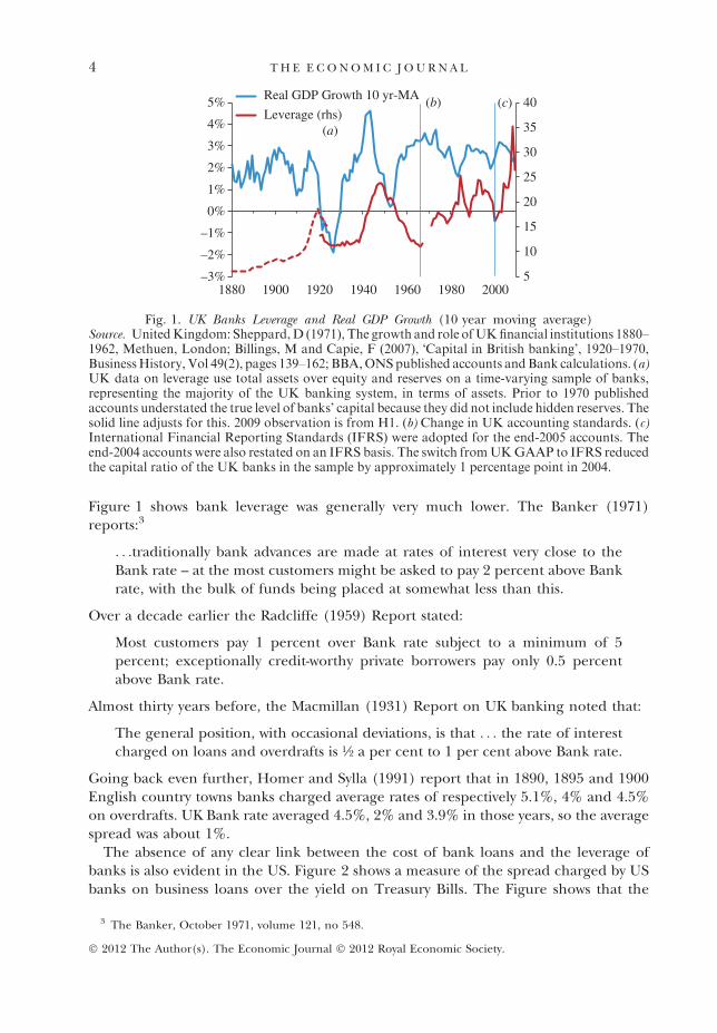
Figure 1 shows bank leverage was generally very much lower. The Banker (1971)reports:3

. . .traditionally bank advances are made at rates of interest very close to theBank rate – at the most customers might be asked to pay 2 percent above Bankrate, with the bulk of funds being placed at somewhat less than this.

Over a decade earlier the Radcliffe (1959) Report stated:

Most customers pay 1 percent over Bank rate subject to a minimum of 5percent; exceptionally credit-worthy private borrowers pay only 0.5 percentabove Bank rate.

Almost thirty years before, the Macmillan (1931) Report on UK banking noted that:

The general position, with occasional deviations, is that . . . the rate of interestcharged on loans and overdrafts is ½ a per cent to 1 per cent above Bank rate.

Going back even further, Homer and Sylla (1991) report that in 1890, 1895 and 1900English country towns banks charged average rates of respectively 5.1%, 4% and 4.5%on overdrafts. UK Bank rate averaged 4.5%, 2% and 3.9% in those years, so the averagespread was about 1%.

The absence of any clear link between the cost of bank loans and the leverage ofbanks is also evident in the US. Figure 2 shows a measure of the spread charged by USbanks on business loans over the yield on Treasury Bills. The Figure shows that the

5

10

15

20

25

30

35

40

–3%

–2%

–1%

0%

1%

2%

3%

4%

5%

1880 1900 1920 1940 1960 1980 2000

Real GDP Growth 10 yr-MA

Leverage (rhs)(a)

(c)(b)

Fig. 1. UK Banks Leverage and Real GDP Growth (10 year moving average)Source. UnitedKingdom: Sheppard,D (1971), The growth and role ofUKfinancial institutions 1880–1962, Methuen, London; Billings, M and Capie, F (2007), �Capital in British banking’, 1920–1970,BusinessHistory, Vol 49(2), pages 139–162; BBA,ONSpublished accounts andBank calculations. (a)UK data on leverage use total assets over equity and reserves on a time-varying sample of banks,representing the majority of the UK banking system, in terms of assets. Prior to 1970 publishedaccounts understated the true level of banks’ capital because they did not include hidden reserves. Thesolid line adjusts for this. 2009 observation is from H1. (b) Change in UK accounting standards. (c)International Financial Reporting Standards (IFRS) were adopted for the end-2005 accounts. Theend-2004 accounts were also restated on an IFRS basis. The switch fromUKGAAP to IFRS reducedthe capital ratio of the UK banks in the sample by approximately 1 percentage point in 2004.

3 The Banker, October 1971, volume 121, no 548.



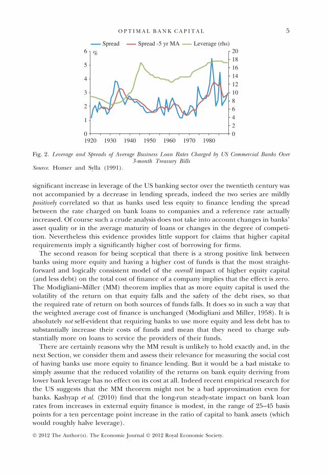
significant increase in leverage of the US banking sector over the twentieth century wasnot accompanied by a decrease in lending spreads, indeed the two series are mildlypositively correlated so that as banks used less equity to finance lending the spreadbetween the rate charged on bank loans to companies and a reference rate actuallyincreased. Of course such a crude analysis does not take into account changes in banks’asset quality or in the average maturity of loans or changes in the degree of competi-tion. Nevertheless this evidence provides little support for claims that higher capitalrequirements imply a significantly higher cost of borrowing for firms.

The second reason for being sceptical that there is a strong positive link betweenbanks using more equity and having a higher cost of funds is that the most straight-forward and logically consistent model of the overall impact of higher equity capital(and less debt) on the total cost of finance of a company implies that the effect is zero.The Modigliani–Miller (MM) theorem implies that as more equity capital is used thevolatility of the return on that equity falls and the safety of the debt rises, so thatthe required rate of return on both sources of funds falls. It does so in such a way thatthe weighted average cost of finance is unchanged (Modigliani and Miller, 1958). It isabsolutely not self-evident that requiring banks to use more equity and less debt has tosubstantially increase their costs of funds and mean that they need to charge sub-stantially more on loans to service the providers of their funds.

There are certainly reasons why the MM result is unlikely to hold exactly and, in thenext Section, we consider them and assess their relevance for measuring the social costof having banks use more equity to finance lending. But it would be a bad mistake tosimply assume that the reduced volatility of the returns on bank equity deriving fromlower bank leverage has no effect on its cost at all. Indeed recent empirical research forthe US suggests that the MM theorem might not be a bad approximation even forbanks. Kashyap et al. (2010) find that the long-run steady-state impact on bank loanrates from increases in external equity finance is modest, in the range of 25–45 basispoints for a ten percentage point increase in the ratio of capital to bank assets (whichwould roughly halve leverage).

02468101214161820

0

1

2

3

4

5

6

1920 1930 1940 1950 1960 1970 1980

Spread Spread -5 yr MA Leverage (rhs)

%

Fig. 2. Leverage and Spreads of Average Business Loan Rates Charged by US Commercial Banks Over3-month Treasury Bills

Source. Homer and Sylla (1991).



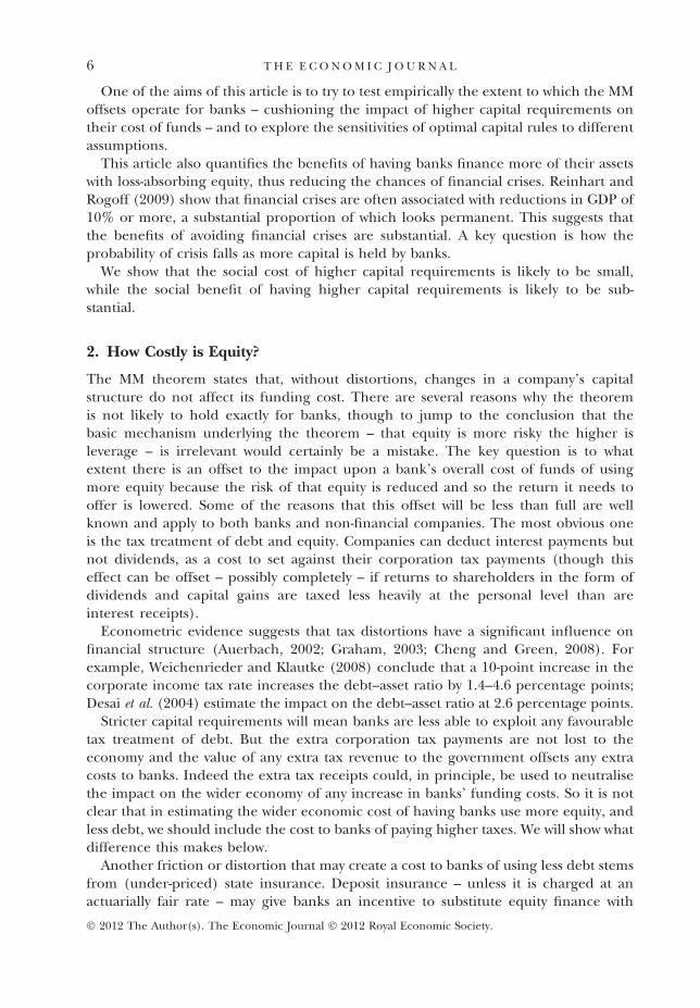
One of the aims of this article is to try to test empirically the extent to which the MMoffsets operate for banks – cushioning the impact of higher capital requirements ontheir cost of funds – and to explore the sensitivities of optimal capital rules to differentassumptions.

This article also quantifies the benefits of having banks finance more of their assetswith loss-absorbing equity, thus reducing the chances of financial crises. Reinhart andRogoff (2009) show that financial crises are often associated with reductions in GDP of10% or more, a substantial proportion of which looks permanent. This suggests thatthe benefits of avoiding financial crises are substantial. A key question is how theprobability of crisis falls as more capital is held by banks.

We show that the social cost of higher capital requirements is likely to be small,while the social benefit of having higher capital requirements is likely to be sub-stantial.

2. How Costly is Equity?

The MM theorem states that, without distortions, changes in a company’s capitalstructure do not affect its funding cost. There are several reasons why the theoremis not likely to hold exactly for banks, though to jump to the conclusion that thebasic mechanism underlying the theorem – that equity is more risky the higher isleverage – is irrelevant would certainly be a mistake. The key question is to whatextent there is an offset to the impact upon a bank’s overall cost of funds of usingmore equity because the risk of that equity is reduced and so the return it needs tooffer is lowered. Some of the reasons that this offset will be less than full are wellknown and apply to both banks and non-financial companies. The most obvious oneis the tax treatment of debt and equity. Companies can deduct interest payments butnot dividends, as a cost to set against their corporation tax payments (though thiseffect can be offset – possibly completely – if returns to shareholders in the form ofdividends and capital gains are taxed less heavily at the personal level than areinterest receipts).

Econometric evidence suggests that tax distortions have a significant influence onfinancial structure (Auerbach, 2002; Graham, 2003; Cheng and Green, 2008). Forexample, Weichenrieder and Klautke (2008) conclude that a 10-point increase in thecorporate income tax rate increases the debt–asset ratio by 1.4–4.6 percentage points;Desai et al. (2004) estimate the impact on the debt–asset ratio at 2.6 percentage points.

Stricter capital requirements will mean banks are less able to exploit any favourabletax treatment of debt. But the extra corporation tax payments are not lost to theeconomy and the value of any extra tax revenue to the government offsets any extracosts to banks. Indeed the extra tax receipts could, in principle, be used to neutralisethe impact on the wider economy of any increase in banks’ funding costs. So it is notclear that in estimating the wider economic cost of having banks use more equity, andless debt, we should include the cost to banks of paying higher taxes. We will show whatdifference this makes below.

Another friction or distortion that may create a cost to banks of using less debt stemsfrom (under-priced) state insurance. Deposit insurance – unless it is charged at anactuarially fair rate – may give banks an incentive to substitute equity finance with



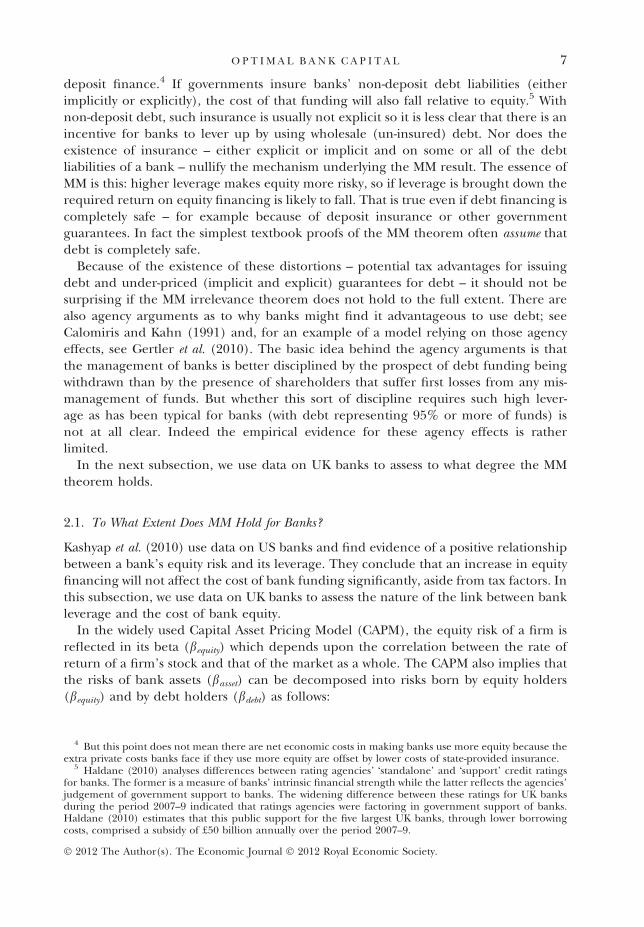
deposit finance.4 If governments insure banks’ non-deposit debt liabilities (eitherimplicitly or explicitly), the cost of that funding will also fall relative to equity.5 Withnon-deposit debt, such insurance is usually not explicit so it is less clear that there is anincentive for banks to lever up by using wholesale (un-insured) debt. Nor does theexistence of insurance – either explicit or implicit and on some or all of the debtliabilities of a bank – nullify the mechanism underlying the MM result. The essence ofMM is this: higher leverage makes equity more risky, so if leverage is brought down therequired return on equity financing is likely to fall. That is true even if debt financing iscompletely safe – for example because of deposit insurance or other governmentguarantees. In fact the simplest textbook proofs of the MM theorem often assume thatdebt is completely safe.

Because of the existence of these distortions – potential tax advantages for issuingdebt and under-priced (implicit and explicit) guarantees for debt – it should not besurprising if the MM irrelevance theorem does not hold to the full extent. There arealso agency arguments as to why banks might find it advantageous to use debt; seeCalomiris and Kahn (1991) and, for an example of a model relying on those agencyeffects, see Gertler et al. (2010). The basic idea behind the agency arguments is thatthe management of banks is better disciplined by the prospect of debt funding beingwithdrawn than by the presence of shareholders that suffer first losses from any mis-management of funds. But whether this sort of discipline requires such high lever-age as has been typical for banks (with debt representing 95% or more of funds) isnot at all clear. Indeed the empirical evidence for these agency effects is ratherlimited.

In the next subsection, we use data on UK banks to assess to what degree the MMtheorem holds.

2.1. To What Extent Does MM Hold for Banks?

Kashyap et al. (2010) use data on US banks and find evidence of a positive relationshipbetween a bank’s equity risk and its leverage. They conclude that an increase in equityfinancing will not affect the cost of bank funding significantly, aside from tax factors. Inthis subsection, we use data on UK banks to assess the nature of the link between bankleverage and the cost of bank equity.

In the widely used Capital Asset Pricing Model (CAPM), the equity risk of a firm isreflected in its beta (bequity) which depends upon the correlation between the rate ofreturn of a firm’s stock and that of the market as a whole. The CAPM also implies thatthe risks of bank assets (basset) can be decomposed into risks born by equity holders(bequity) and by debt holders (bdebt) as follows:

4 But this point does not mean there are net economic costs in making banks use more equity because theextra private costs banks face if they use more equity are offset by lower costs of state-provided insurance.

5 Haldane (2010) analyses differences between rating agencies’ �standalone’ and �support’ credit ratingsfor banks. The former is a measure of banks’ intrinsic financial strength while the latter reflects the agencies’judgement of government support to banks. The widening difference between these ratings for UK banksduring the period 2007–9 indicated that ratings agencies were factoring in government support of banks.Haldane (2010) estimates that this public support for the five largest UK banks, through lower borrowingcosts, comprised a subsidy of £50 billion annually over the period 2007–9.



basset ¼ bequity

E

D þ Eþ bdebt

D

D þ Eð1Þ

D is the debt of the bank; E is its equity. Assuming bdebt = 0, i.e. that the debt is roughlyriskless,6 (1) implies:

bequity ¼D þ E

Ebasset ð2Þ

(D + E) ⁄ E is the ratio of total assets to equity – that is leverage. Equation (2) – whichshows the link between the CAPM and the MM theorem – states that if the beta of bankdebt is zero the risk premium on equity should decline linearly with leverage. When abank doubles its capital ratio (or halves its leverage) – holding the riskiness of thebank’s assets unchanged – the same risks are now spread over an equity cushion that istwice as large. Each unit of equity should only bear half as much risk as before, i.e.equity beta, (bequity), should fall by half. The CAPM would then imply that the riskpremium on that equity – the excess return over a safe rate – should also fall by onehalf. We test to what extent this is true for UK banks.

We first estimate equity betas using publically traded daily stock market returns of UKbanks, together with the returns for the FTSE 100 index, from 1992 to 2010. The banksin our sample are Lloyds TSB (subsequently Lloyds Banking Group), RBS, Barclays,HSBC, Bank of Scotland, Halifax (and subsequently HBOS). For each bank, we obtainits equity beta by regressing its daily stock returns on the daily FTSE returns overdiscrete periods of six months. Figure 3 shows the average of the equity betas acrossbanks for the period 1997–2010.

We regress these estimates of individual banks’ semi-annual equity betas on thebanks’ (start of period) leverage ratio. We want to explore the link between betaand a measure of leverage that is affected by regulatory rules on bank capital.Ideally we would measure leverage as assets relative to the measure of loss-absorbingcapital for which regulators set requirements. Under the Basel III agreements theultimate form of loss-absorbing capital is Common Equity Tier 1 (CET1) capital,which is essentially equity. But it is not possible to get a time series of that measureof capital. So for the regressions we instead define leverage as a bank’s total assetsover its Tier 1 capital. Tier 1 capital includes equity and some hybrid instrumentswhich have more limited loss-absorbing capacity. It is likely that Tier 1 Capital andthe purer measure of loss-absorbing capital defined under Basel III as CET1 moveclosely together so that results we get from any link between the required rate ofreturn on equity and leverage defined using Tier 1 Capital are informative abouthow the required rate of return would move with changes in the amount of trulyloss absorbing capital. (CET1 was about 60% of Basel II Tier 1 equity in 2009, seefootnote 11. But what matters is the impact of a given proportionate change inleverage).

6 The deposit liabilities of banks are close to riskless because of deposit insurance. The assumption of zerorisk is less obviously appropriate for non-deposit debt. But note that what we mean by riskless in the context ofthe CAPM is not that the default probability of debt is zero but the weaker condition that any fluctuation inthe value of debt is not correlated with general market movements.



The regression we estimate is:

bit ¼ X0itb þ eit ;

eit ¼ ai þ lit ;ð3Þ

where, for every bank i = 1, . . ., J at time t = 1, ...,T, bit is the estimated semi-annual equitybeta, Xit is a vector of regressors which include (lagged) leverage and year dummies andb is a vector of parameters.7 ai is a bank-specific effect and lit is an idiosyncraticdisturbance. Equation (2) shows that the coefficient on leverage is an estimate of theasset beta (We also report results from estimating a log specification below.)

Our data set contains observations for a panel of banks at a semi-annual frequencyfrom H1 1997 to H1 2010.8 We use semi-annual estimates of beta since with semiannual published accounts leverage is only measured at that frequency. We showthree estimates for the model: a pooled OLS estimate and two versions whichallow for bank specific effects – the fixed effects (FEs) and random effects (REs)estimators. In choosing between the two estimators which allow for bank specificinfluences on beta the issue is whether the individual effects, ai, are correlated withother regressors. The FE estimator is consistent even if bank specific effects arecorrelated with the regressors Xit. The RE estimator is consistent if the ai aredistributed independently from Xit, in which case it is to be preferred because it ismore efficient.

The data on both beta (Figure 3) and on leverage show some signs of an upwardstrend over the estimation period. If both series are non-stationary (I(1)) then thereis a danger that a levels regression generates a spurious link. We performed Fisher-type unit root test for panels on both beta and leverage. Fisher-type unit root testsare based on augmented Dickey–Fuller tests and can be applied to an unbalancedpanel. The null hypothesis is that all panels contain unit roots and the alternativehypothesis is that at least one panel is stationary. An augmented Dickey–Fuller (ADF)regression including 1 lag and time trend and removing the cross-sectional mean9 –shows that we can reject the null at 0.25% significance level for beta and 1% forleverage. These results seem to suggest that the two series are likely to be trendstationary. Moreover, similar results obtained even when we exclude a time trend inthe ADF regression (the null is rejected at 0.1% for beta and 5% for leverage.) Since

7 It is difficult to assess the impact of changes in the risks of bank assets over time. Including time dummiesin the regressions should allow for factors that impact the average riskiness of bank assets in general from yearto year. That would still leave the impact of shifts in risks of assets that are specific to each bank. We thinkthese might be reflected in a range of factors: the likelihood of incurring losses on its assets as reflected in theprovision for potential losses; on the ease of selling assets without suffering sharp drop in their values; and ontheir overall profitability. We attempt to control for these risks by including the loan loss reserve ratio, theliquid assets ratio and ROA in the regression. But in fact these variables did not appear significant in ourregressions. So in the following discussion, we focus on the results using just leverage and year dummies asregressors.

8 Halifax merged with Bank of Scotland in 2001 to create HBOS. We treat the merged bank HBOS as acontinuation of Halifax and Bank of Scotland stops existing after the merger. This leads to an unbalancedpanel. An unbalanced panel is not a problem for our panel estimation so long as the sample selection processdoes not in itself lead to errors being correlated with regressors. Loosely speaking, the missing values are forrandom reasons rather than systemic ones.

9 We compute for each time period the mean of the series beta and leverage across panels and subtractsthis mean from the series before apply the unit root test. Levin et al. (2002) suggest this procedure to mitigatethe impact of cross-sectional dependence.



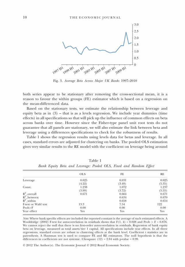
both series appear to be stationary after removing the cross-sectional mean, it is areason to favour the within groups (FE) estimator which is based on a regression onthe mean-differenced data.

Based on the stationary tests, we estimate the relationship between leverage andequity beta as in (3) – that is as a levels regression. We include year dummies (timeeffects) in all specifications so that will pick up the influence of common effects on betaacross banks over time. However since the Fisher-type panel unit root tests do notguarantee that all panels are stationary, we will also estimate the link between beta andleverage using a differences specifications to check for the robustness of results.

Table 1 shows the regression results using levels data for betas and leverage. In allcases, standard errors are adjusted for clustering on banks. The pooled OLS estimationgives very similar results to the RE model with the coefficient on leverage being around

3.0

2.5

2.0

1.5

0.5

0

1997 H1

1999 H1

2001 H1

2003 H1

2005 H1

2007 H1

2009 H1

1.0

Fig. 3. Average Beta Across Major UK Banks 1997–2010

Table 1

Bank Equity Beta and Leverage: Pooled OLS, Fixed and Random Effect

OLS FE RE

Leverage 0.025 0.031 0.025(4.22) (3.49) (5.35)

Const. 1.238 1.072 1.237(3.99) (3.72) (5.55)

R2_overall 0.671 0.664 0.671R2_between 0.634 0.670R2_within 0.658 0.654F-test or Wald test 13.3 7.54 122Prob>F 0.00 0.00 0.00Year effect Yes Yes Yes

Note: Where bank specific effects are included the reported constant is the average of such estimated effects. AWooldridge (2002) F-test for autocorrelation in residuals shows that F(1, 4) = 0.028 and Prob > F = 0.876.We cannot reject the null that there is no first-order autocorrelation in residuals. Regression of bank equitybeta on leverage, measured as total assets ⁄ tier 1 capital. All specifications include year effects. In all threeregressions, standard errors are robust to clustering effects at the bank level. Coefficient t statistics are inparenthesis. A Hausman test is used to compare FE and RE estimators. The null hypothesis is that thedifferences in coefficients are not systemic. Chi-square (12) = 2.84 with p-value = 0.99.



0.025. In the FE regression, changes in leverage have a somewhat bigger impact onequity beta with the coefficient around 0.03. These results suggest that the asset beta ofbanks is low – only around 0.03. This might seem extremely low but it is not at allimplausible. Most bank assets are fixed income claims (loans of various types) and somight be expected to have a very low beta. And an asset beta of only around 0.03generates an equity beta that is close to 1 given that for much of our sample theleverage of banks was around 30.

Given that the FE estimator is consistent both under the null and the alternativehypotheses, we take those as our central estimate – though the difference is not large(a Hausman test is used to compare FE and RE estimators. At standard levels we cannotreject the null hypothesis that the differences in coefficients are not significant(v2(12) = 2.84 with p-value = 0.99)).

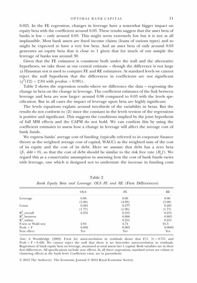
Table 2 shows the regression results where we difference the data – regressing thechange in beta on the change in leverage. The coefficient estimates of the link betweenleverage and beta are now larger: around 0.06 compared to 0.03 with the levels spe-cification. But in all cases the impact of leverage upon beta are highly significant.

The levels equations explain around two-thirds of the variability in betas. But theresults do not conform to (2) since the constant in the levels version of the regressionsis positive and significant. This suggests the conditions implied by the joint hypothesisof full MM effects and the CAPM do not hold. We can confirm this by using thecoefficient estimates to assess how a change in leverage will affect the average cost ofbank funds.

We express banks’ average cost of funding (typically referred to in corporate financetheory as the weighted average cost of capital, WACC) as the weighted sum of the costof its equity and the cost of its debt. Here we assume that debt has a zero beta(b# debt = 0), so that the cost of debt should be similar to the risk free rate (R#f ). Weregard this as a conservative assumption in assessing how the cost of bank funds varieswith leverage, one which is designed not to understate the increase in funding costs

Table 2

Bank Equity Beta and Leverage: OLS FE and RE (First Differences)

OLS FE RE

Leverage 0.06 0.06 0.06(5.00) (4.99) (5.00)

Const. 0.281 0.277 0.281(1.77) (1.90) (1.77)

R2_overall 0.255 0.255 0.255R2_between 0.860 0.863R2_within 0.251 0.251F-test or Wald test 2.94 2.74 35.3Prob > F 0.002 0.003 0.0004Year effect Yes Yes Yes

Note: A Wooldridge (2002) F-test for autocorrelation in residuals shows that F(1, 5) = 0.751 andProb > F = 0.426. We cannot reject the null that there is no first-order autocorrelation in residuals.Regression of bank equity beta on leverage, measured as total assets ⁄ tier 1 capital. Both variables are in theirfirst differences. All specifications include year effects. In all three regressions, standard errors are robust toclustering effects at the bank level. Coefficient t-stat. are in parenthesis.



that lower leverage might bring. By simply assuming away any beneficial impact on thecost of debt from its being made safer as leverage falls we are neutralising one of theroutes through which the MM effects might work. Making this assumption the WACCmay be written as:

WACC ¼ RequityE

D þ Eþ Rf 1� E

D þ E

� �: ð4Þ

The CAPM states that the required return on equity, Requity, can be written as a functionof the equity market risk premium (Rp) and the (bank specific) equity beta:

Requity ¼ Rf þ bequityRp : ð5Þ

Using the coefficients from the FEs levels regression between leverage and bequity and(4) and (5), we get:

Requity ¼ Rf þ ða þ b leverageÞRp : ð6Þ

where a is a constant and b is the coefficient on leverage from the beta regressions.Since b is estimated to be positive, (6) implies that the higher the leverage of a bank thegreater is the required return on its equity.

Total assets of the major UK banks averaged about £6.6 trillion between 2006and 2009; risk-weighted assets (RWAs) were about £2.6 trillion (or 40% of totalassets).10 The average leverage of our banks over that period – that is total assetsover capital (which for the purposes of the regressions we have taken to be Tier 1capital) – is 30. Since CET1 might be only around 60% of Tier 1 capital then leveragedefined as assets to CET1 would have been substantially higher – perhaps averagingaround 50.11

We take 5% as the level of the nominal safe rate; if bdebt = 0 this is also the cost ofbanks raising debt. Five per cent is roughly the average Bank Rate over the 10-yearperiod 1999–2009. It is somewhat higher than the average rate paid on retail deposits ofUK banks but lower than the typical yields on bank bonds over this period. The keything in assessing the impact of a change in capital (or leverage) on banks’ cost offunds is the equity risk premium because it is only the difference between the cost of debtand the required rate of return of equity that matters. So our assumption that thenominal safe rate is 5% is not in any way crucial. We make the 5% assumption about thesafe rate so as to be able to assess whether the required rate of return on bank equitythat our model generates is plausible. We use a market risk premium of 5% as our basecase. This 5% figure is slightly lower than the average excess return of equities over

10 For the banks in our sample RWAs were a slightly lower proportion of total assets than for all UK banks(36% against 40%).

11 According to Table 3 in the BIS Quantitative Impact Study (QIS, BIS (2010c)), the Basel II T1 ratio was10.5%, and the gross CET1 ratio relative to Basel II risk weights was 11.1%, for the QIS sample of large banks(Group 1 banks) at the end of 2009. According to Table 4, �net CET1’ – which we take as reflecting truly loss-absorbing equity – is 41.3% less than gross CET1. Finally, Table 4 suggests that there is an additional effect ofchanges in risk weights of 7.3% that is counted towards the redefinition of equity. Taking all this together, weinfer: (net) CET1 = (11.1 ⁄ 10.5) � [(1 � 0.413) ⁄ (1 + 0.073)] � Basel II T1 = 58% � Basel II T1. We use aconversion of 60% in this article. We used the same source to infer the translation of Basel II RWAs into BaselIII RWAs. According to Table 6 in BIS (2010c), RWAs increased by 23% from Basel II to Basel III for the QISsample of large banks (Group 1 banks) at the end of 2009. We use a conversion of 25% in this article.



government bonds or bills in the UK and the US which for the last 100 years is nearerto 6%. Five per cent is about the average estimate of the equity risk premium of a largesample of economists; see Welch (2001). We show below the implications of using a7.5% risk premium.

Assuming a nominal risk free rate of 5% and a market equity risk premium of 5%,and substituting our FE estimates of a and b from Table 1 into (6), suggests that atleverage of 30 investors require a return on equity of: 5% + (1.07 + 0.03 � 30) � 5% =14.85%.

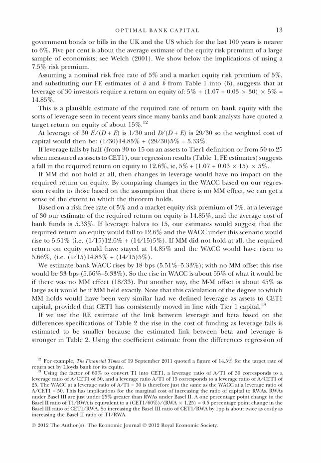
This is a plausible estimate of the required rate of return on bank equity with thesorts of leverage seen in recent years since many banks and bank analysts have quoted atarget return on equity of about 15%.12

At leverage of 30 E ⁄ (D + E) is 1 ⁄ 30 and D ⁄ (D + E) is 29 ⁄ 30 so the weighted cost ofcapital would then be: (1 ⁄ 30)14.85% + (29 ⁄ 30)5% = 5.33%.

If leverage falls by half (from 30 to 15 on an assets to Tier1 definition or from 50 to 25when measured as assets to CET1), our regression results (Table 1, FE estimates) suggestsa fall in the required return on equity to 12.6%, ie, 5% + (1.07 + 0.03 � 15) � 5%.

If MM did not hold at all, then changes in leverage would have no impact on therequired return on equity. By comparing changes in the WACC based on our regres-sion results to those based on the assumption that there is no MM effect, we can get asense of the extent to which the theorem holds.

Based on a risk free rate of 5% and a market equity risk premium of 5%, at a leverageof 30 our estimate of the required return on equity is 14.85%, and the average cost ofbank funds is 5.33%. If leverage halves to 15, our estimates would suggest that therequired return on equity would fall to 12.6% and the WACC under this scenario wouldrise to 5.51% (i.e. (1 ⁄ 15)12.6% + (14 ⁄ 15)5%). If MM did not hold at all, the requiredreturn on equity would have stayed at 14.85% and the WACC would have risen to5.66%, (i.e. (1 ⁄ 15)14.85% + (14 ⁄ 15)5%).

We estimate bank WACC rises by 18 bps (5.51%–5.33%); with no MM offset this risewould be 33 bps (5.66%–5.33%). So the rise in WACC is about 55% of what it would beif there was no MM effect (18 ⁄ 33). Put another way, the M-M offset is about 45% aslarge as it would be if MM held exactly. Note that this calculation of the degree to whichMM holds would have been very similar had we defined leverage as assets to CET1capital, provided that CET1 has consistently moved in line with Tier 1 capital.13

If we use the RE estimate of the link between leverage and beta based on thedifferences specifications of Table 2 the rise in the cost of funding as leverage falls isestimated to be smaller because the estimated link between beta and leverage isstronger in Table 2. Using the coefficient estimate from the differences regression of

12 For example, The Financial Times of 19 September 2011 quoted a figure of 14.5% for the target rate ofreturn set by Lloyds bank for its equity.

13 Using the factor of 60% to convert T1 into CET1, a leverage ratio of A ⁄ T1 of 30 corresponds to aleverage ratio of A ⁄ CET1 of 50, and a leverage ratio A ⁄ T1 of 15 corresponds to a leverage ratio of A ⁄ CET1 of25. The WACC at a leverage ratio of A ⁄ T1 = 30 is therefore just the same as the WACC at a leverage ratio ofA ⁄ CET1 = 50. This has implications for the marginal cost of increasing the ratio of capital to RWAs. RWAsunder Basel III are just under 25% greater than RWAs under Basel II. A one percentage point change in theBasel II ratio of T1 ⁄ RWA is equivalent to a (CET1 ⁄ 60%) ⁄ (RWA � 1.25) = 0.5 percentage point change in theBasel III ratio of CET1 ⁄ RWA. So increasing the Basel III ratio of CET1 ⁄ RWA by 1pp is about twice as costly asincreasing the Basel II ratio of T1 ⁄ RWA.



0.06, (and assuming that the required rate of return on equity at leverage of 30 is14.85%) we find that a having in leverage would reduce the required equity return to10.4%. That implies that the size of the MM offset is about 90% as large as it would beunder full MM (since in this case the rise in the average cost of funds as leverage ishalved is about 3 bps; it would be 33 bps if there were no relation between leverage andthe required return on equity and zero under full MM.).

The results reported in Tables 1 and 2 are based on regressing beta on leverage – anatural specification given (2). But (2) could just as well be estimated in log form.Table 3 shows the log version of (2) where we regress log beta on log leverage. With afull MM effect we would expect the coefficient on log leverage to be 1 – so a doubling inleverage doubles risk. The coefficient estimates in Table 3 are all highly significant butless than 1. The results from the log specification suggest the MM effect is about 70% ofwhat it would be if the MM theorem held precisely.14 This is rather larger than theestimate based on the levels specification, which was that the MM effect was about 45%of the full effect, but it is a bit smaller than the estimate based on differenced data.

Notice that we have assumed no change in the required rate of return on debt asleverage changes. This is a conservative assumption and potentially understates MMeffects. For subordinated wholesale debt which is not covered by deposit insurance, areduction in leverage is likely to reduce the required return on debt – though perhapsonly very marginally. But notice also that, thus far, we have not factored in the impact ofthe tax deductibility of interest payments.

An alternative way to gauge the extent to which the MM effect holds (setting asidetax effects for the moment) is to test more directly the relationship between therequired return on bank equity and bank leverage. This has the advantage of notassuming the CAPM holds. But it is difficult to measure the required return on equity.Ideally, we would like to have expected earnings data for each of the banks in thesample, but we are unable to find a time series of such data. We instead experimentedusing the realised actual earnings over share price (E ⁄ P) as a proxy for required

Table 3

Bank Equity Beta and Leverage (Log Specification)

OLS FE RE

Leverage 0.602 0.692 0.602(6.58) (3.76) (6.81)

Const. �1.405 �1.693 �1.405(�4.45) (�2.69) (�4.35)

R2_overall 0.62 0.66 0.67R2_between 0.54 0.61R2_within 0.64 0.636F or Wald test 13.7 11.3 202Prob > F 0 0 0

Note: Regression of the log of bank equity beta on log leverage, measured as total assets ⁄ tier 1 capital. Yeareffects included. Standard errors are robust to clustering effects at the bank level. Coefficient t-statistic inparenthesis

14 The FE specification generates a point estimate of 0.692 (with a standard error of 0.18). So the rise inrisk is about 70% as great as the MM theory would suggest.



returns and we regress this on leverage. The regression using the earning yield as aproxy for the required return on equity suggests that the impact on the requiredreturn on equity of changing leverage is about as big as if MM held exactly (assumingriskless debt). The beta regressions suggest that the MM theorem effect is somewherebetween 45% and 90% as large as it would be if MM held exactly (depending onwhether we use levels regressions (45%), differenced regressions (90%) or a logspecification (70%)).

In the above calculation we have ignored tax. Arguably if banks pay more tax asleverage falls the value of the extra tax revenue to the government pretty much exactlyoffsets the loss to banks. So from the point of view of measuring true economic costs itshould be ignored. While having sympathy for that argument we will also show belowthe impact of treating tax costs as if they were true costs. In this calculation we willignore any offset from the lower taxation of equity returns to holders of shares; this willgenerate an upper bound of the estimate of the extra cost of banks using more equityand less debt. We will also use as our base case the lowest of the estimates of the MMoffsets from higher leverage, assuming that such offsets are about 45% of what theywould be if MM held exactly.

2.2. Translating Changes in Bank Funding Costs into Changes in Output for the WiderEconomy

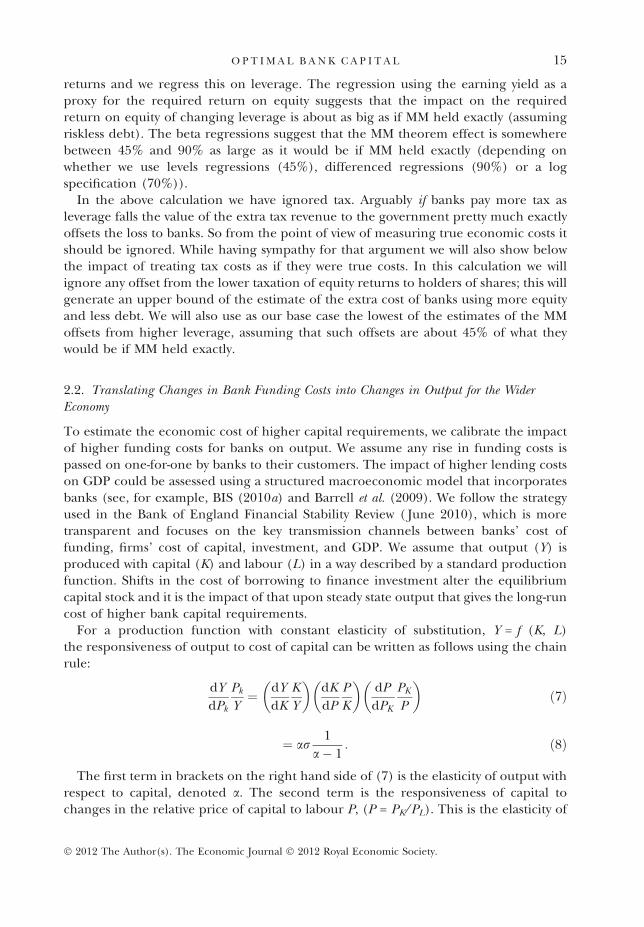
To estimate the economic cost of higher capital requirements, we calibrate the impactof higher funding costs for banks on output. We assume any rise in funding costs ispassed on one-for-one by banks to their customers. The impact of higher lending costson GDP could be assessed using a structured macroeconomic model that incorporatesbanks (see, for example, BIS (2010a) and Barrell et al. (2009). We follow the strategyused in the Bank of England Financial Stability Review ( June 2010), which is moretransparent and focuses on the key transmission channels between banks’ cost offunding, firms’ cost of capital, investment, and GDP. We assume that output (Y) isproduced with capital (K) and labour (L) in a way described by a standard productionfunction. Shifts in the cost of borrowing to finance investment alter the equilibriumcapital stock and it is the impact of that upon steady state output that gives the long-runcost of higher bank capital requirements.

For a production function with constant elasticity of substitution, Y = f (K, L)the responsiveness of output to cost of capital can be written as follows using the chainrule:

dY

dPk

Pk

Y¼ dY

dK

K

Y

� �dK

dP

P

K

� �dP

dPK

PK

P

� �ð7Þ

¼ ar1

a� 1: ð8Þ

The first term in brackets on the right hand side of (7) is the elasticity of output withrespect to capital, denoted a. The second term is the responsiveness of capital tochanges in the relative price of capital to labour P, (P = PK ⁄ PL). This is the elasticity of



substitution between capital and labour (r). The last term is the elasticity of relativeprice with respect to the cost of capital, which we can show is 1 ⁄ (1 � a).15

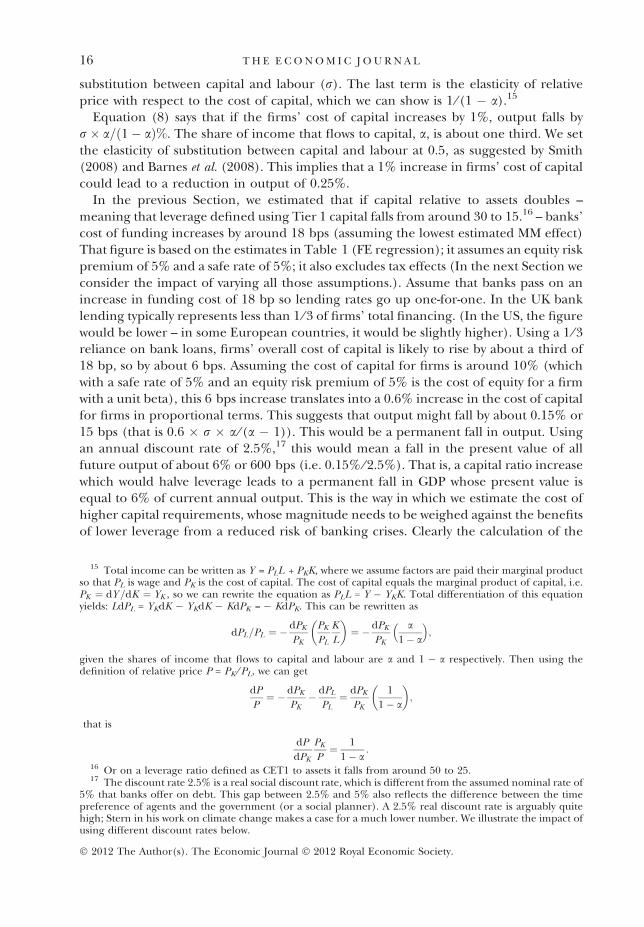
Equation (8) says that if the firms’ cost of capital increases by 1%, output falls byr� a=ð1� aÞ%. The share of income that flows to capital, a, is about one third. We setthe elasticity of substitution between capital and labour at 0.5, as suggested by Smith(2008) and Barnes et al. (2008). This implies that a 1% increase in firms’ cost of capitalcould lead to a reduction in output of 0.25%.

In the previous Section, we estimated that if capital relative to assets doubles –meaning that leverage defined using Tier 1 capital falls from around 30 to 15.16 – banks’cost of funding increases by around 18 bps (assuming the lowest estimated MM effect)That figure is based on the estimates in Table 1 (FE regression); it assumes an equity riskpremium of 5% and a safe rate of 5%; it also excludes tax effects (In the next Section weconsider the impact of varying all those assumptions.). Assume that banks pass on anincrease in funding cost of 18 bp so lending rates go up one-for-one. In the UK banklending typically represents less than 1 ⁄ 3 of firms’ total financing. (In the US, the figurewould be lower – in some European countries, it would be slightly higher). Using a 1 ⁄ 3reliance on bank loans, firms’ overall cost of capital is likely to rise by about a third of18 bp, so by about 6 bps. Assuming the cost of capital for firms is around 10% (whichwith a safe rate of 5% and an equity risk premium of 5% is the cost of equity for a firmwith a unit beta), this 6 bps increase translates into a 0.6% increase in the cost of capitalfor firms in proportional terms. This suggests that output might fall by about 0.15% or15 bps (that is 0.6 � r � a ⁄ (a � 1)). This would be a permanent fall in output. Usingan annual discount rate of 2.5%,17 this would mean a fall in the present value of allfuture output of about 6% or 600 bps (i.e. 0.15% ⁄ 2.5%). That is, a capital ratio increasewhich would halve leverage leads to a permanent fall in GDP whose present value isequal to 6% of current annual output. This is the way in which we estimate the cost ofhigher capital requirements, whose magnitude needs to be weighed against the benefitsof lower leverage from a reduced risk of banking crises. Clearly the calculation of the

15 Total income can be written as Y = PLL + PKK, where we assume factors are paid their marginal productso that PL is wage and PK is the cost of capital. The cost of capital equals the marginal product of capital, i.e.PK ¼ dY =dK ¼ YK , so we can rewrite the equation as PLL = Y � YKK. Total differentiation of this equationyields: LdPL = YKdK � YKdK � KdPK = � KdPK. This can be rewritten as

dPL=PL ¼ �dPK

PK

PK

PL

K

L

� �¼ �dPK

PK

a1� a

� �;

given the shares of income that flows to capital and labour are a and 1 � a respectively. Then using thedefinition of relative price P = PK ⁄ PL, we can get

dP

P¼ �dPK

PK� dPL

PL¼ dPK

PK

1

1� a

� �;

that is

dP

dPK

PK

P¼ 1

1� a:

16 Or on a leverage ratio defined as CET1 to assets it falls from around 50 to 25.17 The discount rate 2.5% is a real social discount rate, which is different from the assumed nominal rate of

5% that banks offer on debt. This gap between 2.5% and 5% also reflects the difference between the timepreference of agents and the government (or a social planner). A 2.5% real discount rate is arguably quitehigh; Stern in his work on climate change makes a case for a much lower number. We illustrate the impact ofusing different discount rates below.



costs of higher bank capital has many moving parts, so before turning to the benefits ofbanks having more capital we consider the sensitivity of costs to alternative assumptions.

2.3. Alternative Scenarios

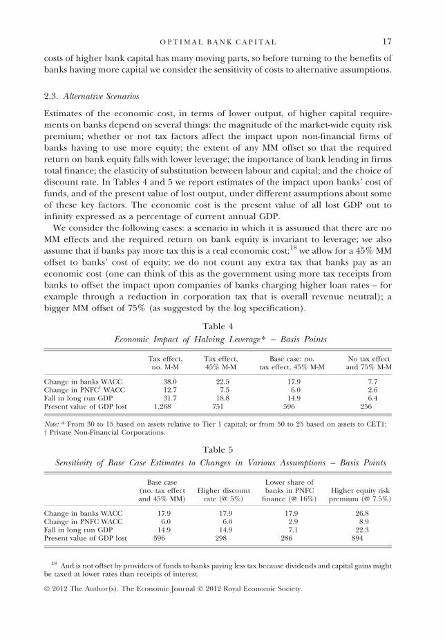
Estimates of the economic cost, in terms of lower output, of higher capital require-ments on banks depend on several things: the magnitude of the market-wide equity riskpremium; whether or not tax factors affect the impact upon non-financial firms ofbanks having to use more equity; the extent of any MM offset so that the requiredreturn on bank equity falls with lower leverage; the importance of bank lending in firmstotal finance; the elasticity of substitution between labour and capital; and the choice ofdiscount rate. In Tables 4 and 5 we report estimates of the impact upon banks’ cost offunds, and of the present value of lost output, under different assumptions about someof these key factors. The economic cost is the present value of all lost GDP out toinfinity expressed as a percentage of current annual GDP.

We consider the following cases: a scenario in which it is assumed that there are noMM effects and the required return on bank equity is invariant to leverage; we alsoassume that if banks pay more tax this is a real economic cost;18 we allow for a 45% MMoffset to banks’ cost of equity; we do not count any extra tax that banks pay as aneconomic cost (one can think of this as the government using more tax receipts frombanks to offset the impact upon companies of banks charging higher loan rates – forexample through a reduction in corporation tax that is overall revenue neutral); abigger MM offset of 75% (as suggested by the log specification).

Table 4

Economic Impact of Halving Leverage * – Basis Points

Tax effect,no. M-M

Tax effect,45% M-M

Base case: no.tax effect, 45% M-M

No tax effectand 75% M-M

Change in banks WACC 38.0 22.5 17.9 7.7Change in PNFCy WACC 12.7 7.5 6.0 2.6Fall in long run GDP 31.7 18.8 14.9 6.4Present value of GDP lost 1,268 751 596 256

Note: * From 30 to 15 based on assets relative to Tier 1 capital; or from 50 to 25 based on assets to CET1;y Private Non-Financial Corporations.

Table 5

Sensitivity of Base Case Estimates to Changes in Various Assumptions – Basis Points

Base case(no. tax effectand 45% MM)

Higher discountrate (@ 5%)

Lower share ofbanks in PNFC

finance (@ 16%)Higher equity risk

premium (@ 7.5%)

Change in banks WACC 17.9 17.9 17.9 26.8Change in PNFC WACC 6.0 6.0 2.9 8.9Fall in long run GDP 14.9 14.9 7.1 22.3Present value of GDP lost 596 298 286 894

18 And is not offset by providers of funds to banks paying less tax because dividends and capital gains mightbe taxed at lower rates than receipts of interest.



The impact of a doubling in capital (halving in leverage) is to increase the averagecost of bank funds by about 38 bps when there is no MM offset and we assume that allof the impact of the extra tax paid by banks is included as an economic cost. Thatwould reduce the present value of the flow of annual GDP by 13% of current annualoutput (1,268 basis points); it would mean the level of GDP was permanently about onethird of a percent lower. If we allow a 45% MM offset the impact on bank cost of fundsfalls to about 22 bps and the effect on GDP falls to under 0.2% (generating a presentvalue loss of about 7.5% of annual GDP). Of that impact on WACC just under 5 bps is atax effect; the effect of higher capital on WACC without tax is slightly under 18 bps,generating a hit to GDP of about 0.15% (creating a present value loss of just under6%). If the MM effect is bigger (75%) the rise in WACC falls to around 8 bps and thefall in long run level of GDP is just over 6 bps.

Table 5 shows the impact of varying other assumptions relevant to the impact uponGDP of higher bank funding costs. Here we use the base case assumptions (column 3of Table 4) on MM and tax effects. If we double the discount rate (from 2.5% to 5%) thepresent value of lost output is halved. If instead of assuming that non-financial com-panies finance 33% of investment with bank loans we set that rate at 16% (closer to therecent average in the UK) the impact of higher capital upon GDP is also roughly halved.But raising the overall market equity risk premium from 5% to 7.5% rather substantiallyraises the cost of higher bank capital – which is about 50% higher than in the base case.

These estimates illustrate that under reasonable assumptions even doubling theamount of bank capital has a relatively modest impact upon the average cost of bankfunds – ranging from just under 40 bps to under 10 bps. If we allowed the cost of debtraised by banks to fall with leverage, the estimated cost of higher capital would be evensmaller. One reason why the cost of bank debt may not be responsive to changes inleverage may be its implicit insurance by the government. We do not attempt to makeany explicit calculation of the value of such insurance but its existence only reinforcesthe argument for higher capital requirements to be imposed on banks.

3. Quantifying the Benefits of Higher Capital Requirements

Higher capital makes banks better able to cope with variability in the value of theirassets without triggering fears of (and actual) insolvency. This should lead to a morerobust banking sector and a lower frequency of banking crises. The benefit of havinghigher capital levels can be measured as the expected cost of a financial crisis that hasbeen avoided. The marginal benefit of having banks fund more of their assets usingequity is the reduction in the probability of a banking crisis that using more equitybrings multiplied by the expected cost of a banking crisis. In this Section, we try tocalibrate how much the chances of banking crises are reduced as bank capital ratios riseand how costly such crises typically are. Both those things are hard to judge.

3.1. Probability of Crisis and Bank Capital

We think of a banking crisis – at least of the sort that higher capital can counter – as asituation where many banks come close to insolvency. That is where the fall in the valueof their assets is close to being as large as (or is greater than) the amount of



loss-absorbing equity capital they have. The type of fluctuations in asset values thatwould generate such a situation are generalised falls in the value of bank assets – thingsnot specific to a particular bank. The key assumption we make is that generalised fallsin the value of bank assets are driven by changes in the level of incomes in theeconomy. More specifically we will assume that losses arise if income levels fall. Thisassumption is consistent with the evidence from periods when banks have sufferedsubstantial losses on the value of their assets. We review that evidence in Appendix Band use it to calibrate the link between falls in incomes in the economy and declines inthe value of bank assets. Our calibration is conservative, in the sense that the sensitivitywe assume between falls in incomes in the economy and declines in the value of bankassets is at the low end of what recent experience suggests. The evidence suggests thatin recessions that are associated with banking crises the proportionate fall in the valueof (un-weighted) bank assets is often equal to the decline in GDP. We assume that thefall in bank assets for a given fall in incomes is only about half as large as that.

We proceed by modelling the process that drives incomes. Given the assumed linkbetween those fluctuations and the value of bank assets we can calculate the probabilitydistribution of asset values and find the probabilities that asset values fall by more thanthe level of bank equity. That is the probability of a banking crisis. From that it is asimple calculation to see how the probability of insolvency changes, for given assets, asbank equity rises. The product of that change in the probability in insolvency and thecost of insolvency is the marginal benefit of banks using more equity.

The key parts of the mechanism can be illustrated with three equations. Denote theprobability of a bank’s insolvency by p, losses on bank assets by L, bank equity by K (forcapital), percentage changes in income levels in the economy by Y, and the cost ofbanking crises (insolvency) by C. The relationships that govern the marginal benefit ofhaving banks use more equity (denoted MB) are these:

p ¼ probðL > K Þ ð9Þ

L ¼ f ðY Þ > 0 if Y < 0 with f 0ðY Þ < 00 if Y � 0

�ð10Þ

MB ¼ ðdp=dK Þ � C ð11Þ

For any given level of K there is a value of Y, denoted Y *, such that if falls in incomesare greater than this level then L exceeds K. This means that Y *<0 and f (Y *) = K. Theprobability of a crisis for a given level of capital is prob(Y < Y *). If we model theprobability distribution of changes in incomes then given a model of the link betweenchanges in income and asset values (that is the f (Y ) function) we can calculate thatlevel of Y* and the probability that Y < Y *. Clearly dY * ⁄ dK < 0 and so dp ⁄ dK < 0.

The crucial assumption is that bank asset values are driven by the incomes of thosewho have borrowed from banks. A large part of banks’ assets are debt contracts whosevalue depends on the ability of borrowers to honour interest and principal repaymentsfrom their income and savings. There is likely to be a close link between the value ofbank assets (in aggregate) and a country’s national income (GDP). The more inter-national are banks the less tight will be the link between movements in domestic



incomes and the value of bank assets. A few UK banks do have a great many foreignassets. It is also the case that sharp recessions – the ones where bank capital reallymatters – are often synchronised across countries.

Our basic assumption is that losses in the value of assets are linked to permanent fallsin GDP.19 Specifically we will assume that the percentage fall in the value of RWAsmoves in line with any permanent fall in the level of per capita GDP. In aggregate oursample of big UK banks have had total assets that are almost three times RWAs on theBasel II definitions. The Basel III measures of RWA are greater than the Basel IImeasures by a little under 25%; see BIS (2010c, Table 6). On a Basel III definition ofRWA the total assets of major UK banks are probably closer to 2.25 times RWA. So on aBasel III RWA definition the typical risk weight is about 45%. We assume that a banksees a fall in the value of each of its assets that is equal to any permanent fall in percapita GDP (in per cent) multiplied by the risk weight of that asset. If per capita GDPpermanently falls by 1% an asset worth £1 and with a risk weight of 0.45 would see itsvalue fall by 0.45%, so it would be worth 99.55p. If GDP fell by 10% in a year (a verylarge fall), and using the average risk weight of 0.45, the fall in assets would be 4.5% –so assets would be worth 95.5% of their start of year value. A bank with leverage lessthan 22.2 (1 ⁄ 0.045) would have enough capital to absorb this loss.

In terms of the notation used above – and now interpreting Y as the percentagechange in per capita GDP – we are assuming a specific functional form for equation(10), namely:

L ¼ jY j � RWA if Y < 0

L ¼ 0 if Y > 0;

which implies that bankruptcy occurs if Y < � K ⁄ RWA.One way to think about this assumption – that RWAs fall by the same as a fall in

average incomes – is to see assets with a positive risk weight as ones where the ability ofthe borrower to repay the loan is less than certain and depends on their income. Morespecifically, assume that an asset with a risk weight of 0 is always repaid but that an assetwith the average risk weight (relative to all those which are judged risky) has arepayment profile which is eroded in line with falls in average incomes in the economy.So an average risky asset is one which, so long as average incomes do not fall, is repaidin full; but if income falls x% the value of interest and capital repayments also falls byx%. This would imply that risky agents who have borrowed from banks and find thattheir incomes fall cannot devote more of their lower incomes to debt repayment.

This way of looking at the assumption we make of the link between falls in incomesand in the value of RWAs helps in interpretation but it does not in itself throw muchlight on its consistency with the evidence. So in Appendix B we describe the evidenceon the relative size of recent falls in banks’ assets and falls in GDP. We find that in

19 Our empirical model of changes in GDP is a random walk with drift and a stochastic term which has amixed distribution. This model implies that changes in GDP are permanent and that there is a unit root inGDP. Evidence on whether there is a unit root in GDP is not entirely conclusive though many papers do findsupport for the unit root hypothesis; see the influential original contribution of Nelson and Plosser (1982)and later work by Campbell and Mankiw (1995), Perron (1988), Banerjee et al. (1992). Fleissig and Strauss(1999) find some evidence for trend stationarity using panel unit root tests.



recessions that are associated with banking crises the fall in the value of (un-weighted)bank assets is often equal to the decline in GDP. It is very likely that the proportionatefall in RWAs is greater than the decline in total assets because risky assets are moreexposed to falls in incomes. In recent years Basel III measures of RWA would probablyhave been a bit under 1 ⁄ 2 of total assets for large UK banks.20 So if – as some evidenceseems to suggest – declines in total assets are of roughly the same order as declines inGDP, then the proportionate fall in RWA should be expected to be greater – perhapstwice as great.21 This is why we consider our assumption of an equal percentage fall inRWAs and GDP as a conservative one for calibrating the exposure of bank assets toeconomy wide shocks.

Based on this assumption, we use an assumed probability distribution for changes inannual GDP to calculate the probability of a banking crisis in any given year for dif-ferent levels of bank capital. We note that it is far from self-evident that using one yearas the appropriate time interval is correct. What we are assuming is that within a yearbanks find it hard to raise their level of capital so that if a shock arises within a yearwhich generates losses greater than capital at the start of the year then this will cause abanking crisis.

We are taking falls in incomes as the fundamental driver of losses on bank assets. Weare treating this as an exogenous factor. So ideally we need to model those shocks toincomes that are not themselves influenced by banking problems. This is notstraightforward since some of the historical fluctuations in incomes will have beeninfluenced by banking problems. We use a dataset of income fluctuations which webelieve means that this feedback (from initial shocks in incomes that are influencedand exacerbated by the banking problems they may generate) is likely to be absent orinsignificant in the great majority of observations. We think that our way of modellingGDP largely reflects shocks that cause bank asset values to fluctuate – rather thanshocks that emanate from banks and cause movements in incomes.22 What we do is tocalibrate a model of shocks to incomes (per capita GDP) using data from a large groupof countries over a nearly two hundred year period. For many of these countries, andfor much of the period, banks were much less important than they have subsequentlybecome and most of the biggest movements in GDP reflect wars and political turmoilthat are likely to be substantially independent from banking conditions. (In estimatingoptimal bank capital we will not however assume that banks need to be able to with-stand extreme events like wars.)

Historical data on changes in GDP strongly suggests that the frequency of such largenegative shocks is very much greater than would be implied by an estimated normaldistribution, a distribution which most of the time matches the GDP data well. A much

20 Basel III RWA are about 25% larger than Basel II RWA. They are therefore a larger share of total assetsthan are RWA under Basel II, as well as better reflecting the relative risk of assets. That is why we think ourresults on optimal bank capital relative to RWA should be interpreted in terms of Basel III RWA.

21 Consider an extreme example where there are two types of assets: those that are risky and those that arecompletely safe. If RWAs are 45% of total assets then if total assets are 100, those exposed to risk are worth 45.By assumption all the falls are concentrated in the risky assets. If total assets fall in line with falls with GDPthen the value of risky assets needs to fall by about 2.2% for each 1% fall in GDP (i.e. by 1 ⁄ 0.45%).

22 Even so it is likely that some of the historical variability in GDP reflects the impact of banking problems.To the extent this is true it increases the benefits of having banks hold more equity because that will result in asomewhat lower variance of GDP. In ignoring this feedback we are therefore likely to underestimate the sizeof optimal bank capital.



better way to match the distribution of risks that end up affecting GDP is to assume thatmost of the time risks – or shocks – follow a normal distribution but once every fewdecades a shock comes that is very large and which is not a draw from a normal dis-tribution. This assumption – that GDP changes are normal but with the added chancethat there are low probability quite extreme outcomes – is one made by Robert Barro(2006) in a series of important studies of rare events that hit economies.

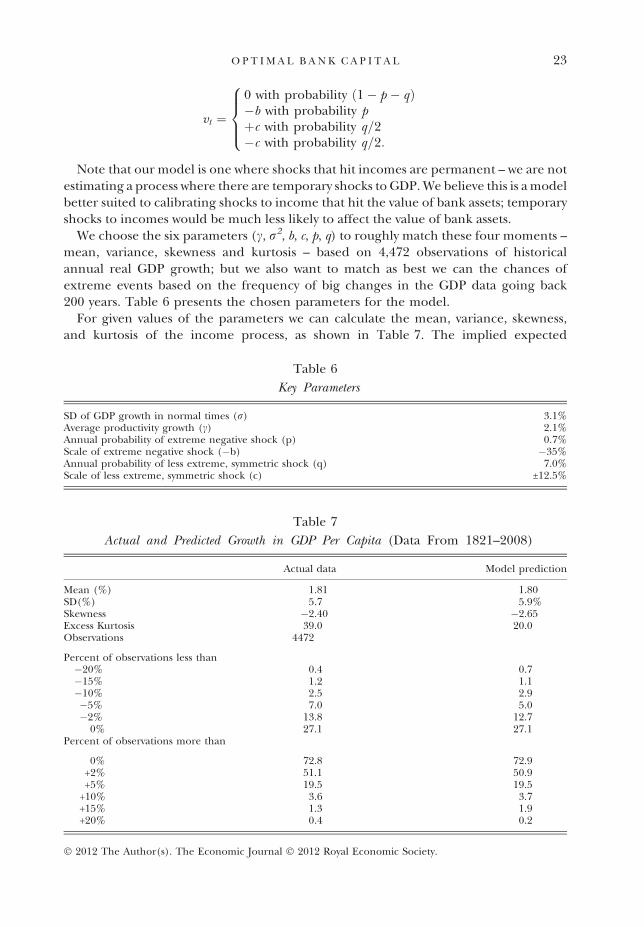
Figure 4 shows a slight generalisation of the Barro (2006) model calibrated tomatch historical experience going back almost 200 years. The data are for the changein GDP per capita for a sample of 31 countries and starts, in some cases, in 1821 andcomes up to 2008. We do not include observations from 2009 and 2010 when GDP inmost countries was severely affected by the global banking crisis which began in thewake of the failure of Lehman Brothers in September 2008. We have almost 4,500observations of annual GDP growth across the sample of countries; see Appendix Afor more details and also Miles et al. (2005). Here we assume that the first differenceof the log of per capita GDP (Y ) follows a random walk with a drift and two randomcomponents

ðYtÞ ¼ cþ ut�1 þ vt�1:

The parameter c captures average productivity growth. The first random component, ut

is the shock in normal times, i.e. it reflects the typical level of economic volatility. Thisshock follows an independently and normally distributed process u � N(0, r2).

The other random component vt is zero in normal times but with given probabilitiesit takes on significant values. There is a small chance (probability p) that vt takes on avery large negative value, equal to �b. The parameter b represents the scale of theasymmetric shock; there is no chance of an equally large positive shock. There is asecond type of shock, which is symmetric, and whose scale is denoted by c. This shockhas a higher probability of occurring (probability q > p) and it is smaller, though stilllarge relative to the volatility of the normally distributed shock. Formally, the randomcomponent vt can be written as following

0

0.02

0.04

0.06

0.08

0.10

0.12

0.14

–40 –35 –30 –25 –20 –15 –10 –5 0 5 10 15 20 25 30 35 40

Frequency Distribution ofChanges in GDP -Actual Data

Predicted by the Model(Base Case)

Probability

100 Times Annual Change in Log GDP

Fig. 4. Annual GDP Growth: Comparing the Economic Model with Data (1821–2008)



vt ¼

0 with probability ð1� p � qÞ�b with probability pþc with probability q=2�c with probability q=2:

8>><>>:

Note that our model is one where shocks that hit incomes are permanent – we are notestimating a process where there are temporary shocks to GDP. We believe this is a modelbetter suited to calibrating shocks to income that hit the value of bank assets; temporaryshocks to incomes would be much less likely to affect the value of bank assets.

We choose the six parameters (c, r2, b, c, p, q) to roughly match these four moments –mean, variance, skewness and kurtosis – based on 4,472 observations of historicalannual real GDP growth; but we also want to match as best we can the chances ofextreme events based on the frequency of big changes in the GDP data going back200 years. Table 6 presents the chosen parameters for the model.

For given values of the parameters we can calculate the mean, variance, skewness,and kurtosis of the income process, as shown in Table 7. The implied expected

Table 7

Actual and Predicted Growth in GDP Per Capita (Data From 1821–2008)

Actual data Model prediction

Mean (%) 1.81 1.80SD(%) 5.7 5.9%Skewness �2.40 �2.65Excess Kurtosis 39.0 20.0Observations 4472

Percent of observations less than�20% 0.4 0.7�15% 1.2 1.1�10% 2.5 2.9�5% 7.0 5.0�2% 13.8 12.7

0% 27.1 27.1Percent of observations more than

0% 72.8 72.9+2% 51.1 50.9+5% 19.5 19.5

+10% 3.6 3.7+15% 1.3 1.9+20% 0.4 0.2

Table 6

Key Parameters

SD of GDP growth in normal times (r) 3.1%Average productivity growth (c) 2.1%Annual probability of extreme negative shock (p) 0.7%Scale of extreme negative shock (�b) �35%Annual probability of less extreme, symmetric shock (q) 7.0%Scale of less extreme, symmetric shock (c) ±12.5%



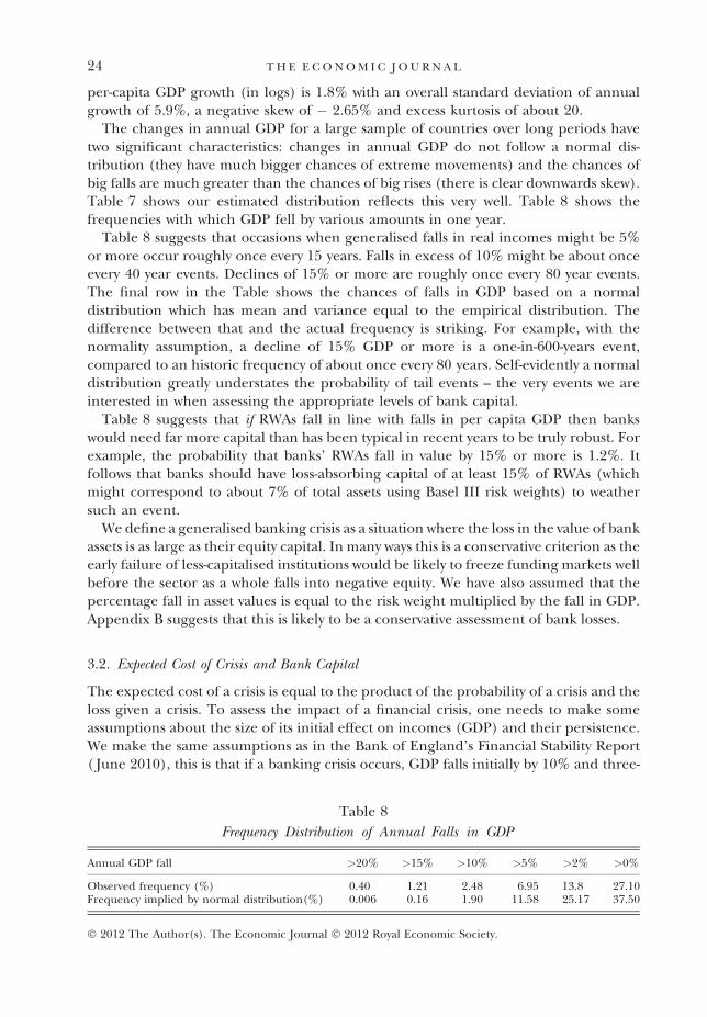
per-capita GDP growth (in logs) is 1.8% with an overall standard deviation of annualgrowth of 5.9%, a negative skew of � 2.65% and excess kurtosis of about 20.

The changes in annual GDP for a large sample of countries over long periods havetwo significant characteristics: changes in annual GDP do not follow a normal dis-tribution (they have much bigger chances of extreme movements) and the chances ofbig falls are much greater than the chances of big rises (there is clear downwards skew).Table 7 shows our estimated distribution reflects this very well. Table 8 shows thefrequencies with which GDP fell by various amounts in one year.

Table 8 suggests that occasions when generalised falls in real incomes might be 5%or more occur roughly once every 15 years. Falls in excess of 10% might be about onceevery 40 year events. Declines of 15% or more are roughly once every 80 year events.The final row in the Table shows the chances of falls in GDP based on a normaldistribution which has mean and variance equal to the empirical distribution. Thedifference between that and the actual frequency is striking. For example, with thenormality assumption, a decline of 15% GDP or more is a one-in-600-years event,compared to an historic frequency of about once every 80 years. Self-evidently a normaldistribution greatly understates the probability of tail events – the very events we areinterested in when assessing the appropriate levels of bank capital.

Table 8 suggests that if RWAs fall in line with falls in per capita GDP then bankswould need far more capital than has been typical in recent years to be truly robust. Forexample, the probability that banks’ RWAs fall in value by 15% or more is 1.2%. Itfollows that banks should have loss-absorbing capital of at least 15% of RWAs (whichmight correspond to about 7% of total assets using Basel III risk weights) to weathersuch an event.

We define a generalised banking crisis as a situation where the loss in the value of bankassets is as large as their equity capital. In many ways this is a conservative criterion as theearly failure of less-capitalised institutions would be likely to freeze funding markets wellbefore the sector as a whole falls into negative equity. We have also assumed that thepercentage fall in asset values is equal to the risk weight multiplied by the fall in GDP.Appendix B suggests that this is likely to be a conservative assessment of bank losses.

3.2. Expected Cost of Crisis and Bank Capital

The expected cost of a crisis is equal to the product of the probability of a crisis and theloss given a crisis. To assess the impact of a financial crisis, one needs to make someassumptions about the size of its initial effect on incomes (GDP) and their persistence.We make the same assumptions as in the Bank of England’s Financial Stability Report( June 2010), this is that if a banking crisis occurs, GDP falls initially by 10% and three-

Table 8

Frequency Distribution of Annual Falls in GDP

Annual GDP fall >20% >15% >10% >5% >2% >0%

Observed frequency (%) 0.40 1.21 2.48 6.95 13.8 27.10Frequency implied by normal distribution(%) 0.006 0.16 1.90 11.58 25.17 37.50



quarters of this reduction lasts for just five years whilst one quarter is permanent. Basedon that assumption, and a discount rate of 2.5%, the present value gain of permanentlyreducing the likelihood of a systematic crisis in any one year by one percentage point isaround 55% of current annual GDP.23 The initial impact of a 10% fall in GDP is in linewith the IMF estimate of the typical cost of a financial crisis. It also accords with therecent experience of the UK: the level of UK GDP in the first half of 2010 was around10% below what it would have been if growth from 2007 H1 had been equal to the long-run UK average.

The estimate of the cost of crisis is, of course, sensitive to our assumptions about theimpact of the financial shock and its persistence. If we assumed no permanent effectson GDP, the benefits of higher capital requirements would then fall to about 20% ofGDP per percentage point reduction in the likelihood of crises. The cost of bank criseswould be very much greater if we assumed that all the damage done was permanent. Insome ways that would be the natural assumption to make since it is consistent with theassumed process for GDP we have used, which is a random walk. We are effectivelymaking the assumption that most shocks which have historically hit countries (the greatmajority of which are not banking crises) have permanent effects but that bank crisesgenerate big shocks to output, not all of which are permanent. We make thisassumption to avoid the charge of pushing the results towards generating very highoptimal capital.

4. Calibrating Optimal Capital

Using the estimates for the social costs and benefits of higher capital requirements, wecan assess what is a socially-optimal level of capital for the banking sector; that is thelevel of capital where the extra benefit of having more capital just falls to the extra costsof having more capital.

The marginal benefit of additional units of equity capital is the reduction in theexpected cost of future financial crises. We measure capital relative to RWAs and weassume that any losses on RWA is in proportion to any fall in per capita GDP. We havedefined a crisis as a situation where bank equity is wiped out. This means that the losson assets – the value of which we assume is RWA multiplied by the percentage declinein per capita GDP – exceeds equity capital. If we express capital relative to RWA then acrisis happens when the percentage fall in per capita GDP exceeds that ratio. So ifcapital is 15% of RWA a decline in per capita GDP of 15% causes a banking crisis. Giventhe assumed distribution of shocks to bank asset values, the benefit of greater equity

23 The expected loss in output per crisis, LPC, can then be computed as

LPC ¼ 34

1�d5

1�d þ 14

11�d

� �� 10%

where d is the discount factor. Using a discount rate of 2.5% (which implies a discount factor of 0.975), this amountsto a cumulated discounted cost of about 140% of GDP per crisis, and 1.4% of GDP per percentage point reductionin the likelihood of this crisis. As higher capital requirements would not only reduce the likelihood of a single crisisbut of all future crises, the expected benefit of higher capital requirements would be

1% LPC 11�d

per percentage point reduction in the probability of crises, or about 55% of GDP. A similar approach is used inHaldane (2010).



capital in reducing the chances of a banking crisis tends to decline with additionalcapital. But since it looks like there are very occasionally extremely negative shocks toasset values, the benefit of extra capital does not fall monotonically. The costs of havingbanks finance more of their assets with equity is, given our assumptions, linear. So themarginal cost (for a given set of assumptions on the equity risk premium, the extent towhich MM holds and the degree to which investment is assumed to be financed frombank lending) is constant. Both costs and benefits are measured as the expected pre-sent value of all changes to the future levels of GDP.

In Figure 5 we show two estimates of the marginal benefits of extra capital: in thehigher line we assume that a quarter of the fall in output associated with a financialcrisis is permanently lost; in the lower line we assume that five years after a bankingcrisis the level of GDP returns to where it would have been had there been no crisis.

On the horizontal axis in this Figure we show the ratio of capital to RWAs. Incalibrating the model we need to be clear about what we mean by capital and RWAs. Wehave consistently said that capital needs to be pure, loss-absorbing capital. We think ofthis as common equity. So the regulatory concept nearest to it would seem to be theBasel III concept of CET1. In measuring the cost of requiring more equity relative toRWA we need to translate a change in that capital ratio to a rise in banks’ weightedaverage cost of funds.24

0%

1%

2%

3%

4%

5%

6%

7%

8%

9%

10%

0% 5% 10% 15% 20% 25% 30% 35% 40% 45% 50% 55% 60%

Marginal Cost (Range of Estimates)

Marginal Cost (Base Case)

Marginal Benefit (No Permanent Effect)

Marginal Benefit (Base Case)

Capital Ratio

Proportion of GDP

Fig. 5. Expected Marginal Costs and Benefits of More Capital

24 It is useful to explain how we estimate the cost of higher capital ratios (in terms of lost GDP) byreference to the figures in Table 4. That table showed that on the base case assumptions halving leverage –reducing assets to Tier 1 capital from 30 to 15 – costs 596 bp of lost GDP, in present value terms. Basel II RWAwere, for big UK banks, about 40% of total assets, so assets to Basel II RWA (which we denote A ⁄ RWA2) wasaround 250%. We assume that CET1 is around 0.6 a large as Tier 1 capital and that RWA under Basel III arearound 1.25 as large as under Basel II. Using those assumptions the shift in leverage from 30 to 15 is a changein the Basel III capital ratio (ie CET1 to Basel III RWA) from:

0:6=30� ½A=ðRWA2� 1:25Þ� to 0:6=15 � ½A=ðRWA2� 1:25Þ�

Since A ⁄ RWA2 is around 2.5 this is a change from 4.0% to about 8.0%. So to convert into a cost per unit of capital toRWA we need to use: 596 bp ⁄ 4.064 = 149 bp. This is what we use for the base case. Lower and higher cost scenariosare similarly scaled.



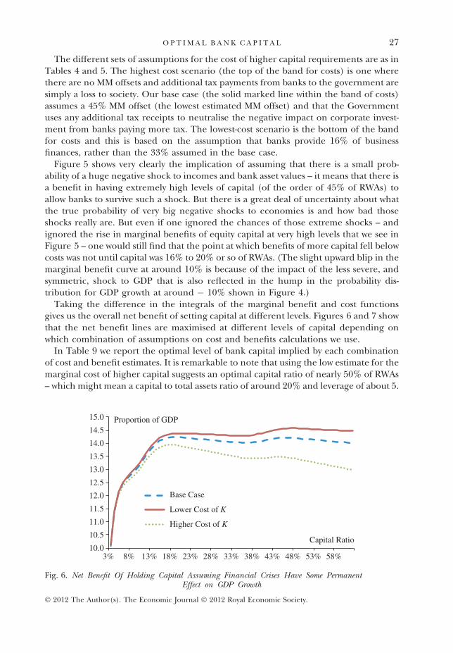
The different sets of assumptions for the cost of higher capital requirements are as inTables 4 and 5. The highest cost scenario (the top of the band for costs) is one wherethere are no MM offsets and additional tax payments from banks to the government aresimply a loss to society. Our base case (the solid marked line within the band of costs)assumes a 45% MM offset (the lowest estimated MM offset) and that the Governmentuses any additional tax receipts to neutralise the negative impact on corporate invest-ment from banks paying more tax. The lowest-cost scenario is the bottom of the bandfor costs and this is based on the assumption that banks provide 16% of businessfinances, rather than the 33% assumed in the base case.

Figure 5 shows very clearly the implication of assuming that there is a small prob-ability of a huge negative shock to incomes and bank asset values – it means that there isa benefit in having extremely high levels of capital (of the order of 45% of RWAs) toallow banks to survive such a shock. But there is a great deal of uncertainty about whatthe true probability of very big negative shocks to economies is and how bad thoseshocks really are. But even if one ignored the chances of those extreme shocks – andignored the rise in marginal benefits of equity capital at very high levels that we see inFigure 5 – one would still find that the point at which benefits of more capital fell belowcosts was not until capital was 16% to 20% or so of RWAs. (The slight upward blip in themarginal benefit curve at around 10% is because of the impact of the less severe, andsymmetric, shock to GDP that is also reflected in the hump in the probability dis-tribution for GDP growth at around � 10% shown in Figure 4.)

Taking the difference in the integrals of the marginal benefit and cost functionsgives us the overall net benefit of setting capital at different levels. Figures 6 and 7 showthat the net benefit lines are maximised at different levels of capital depending onwhich combination of assumptions on cost and benefits calculations we use.

In Table 9 we report the optimal level of bank capital implied by each combinationof cost and benefit estimates. It is remarkable to note that using the low estimate for themarginal cost of higher capital suggests an optimal capital ratio of nearly 50% of RWAs– which might mean a capital to total assets ratio of around 20% and leverage of about 5.

10.0

10.5

11.0

11.5

12.0

12.5

13.0

13.5

14.0

14.5

15.0

3% 8% 13% 18% 23% 28% 33% 38% 43% 48% 53% 58%

Base Case

Higher Cost of K

Lower Cost of K

Proportion of GDP

Capital Ratio

Fig. 6. Net Benefit Of Holding Capital Assuming Financial Crises Have Some PermanentEffect on GDP Growth



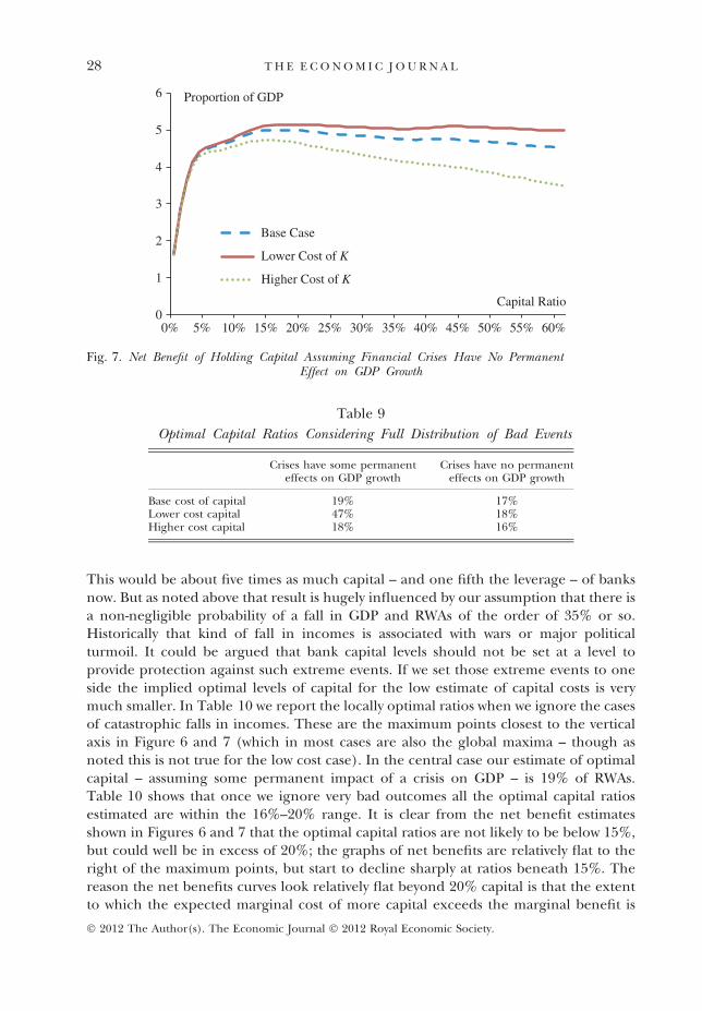
This would be about five times as much capital – and one fifth the leverage – of banksnow. But as noted above that result is hugely influenced by our assumption that there isa non-negligible probability of a fall in GDP and RWAs of the order of 35% or so.Historically that kind of fall in incomes is associated with wars or major politicalturmoil. It could be argued that bank capital levels should not be set at a level toprovide protection against such extreme events. If we set those extreme events to oneside the implied optimal levels of capital for the low estimate of capital costs is verymuch smaller. In Table 10 we report the locally optimal ratios when we ignore the casesof catastrophic falls in incomes. These are the maximum points closest to the verticalaxis in Figure 6 and 7 (which in most cases are also the global maxima – though asnoted this is not true for the low cost case). In the central case our estimate of optimalcapital – assuming some permanent impact of a crisis on GDP – is 19% of RWAs.Table 10 shows that once we ignore very bad outcomes all the optimal capital ratiosestimated are within the 16%–20% range. It is clear from the net benefit estimatesshown in Figures 6 and 7 that the optimal capital ratios are not likely to be below 15%,but could well be in excess of 20%; the graphs of net benefits are relatively flat to theright of the maximum points, but start to decline sharply at ratios beneath 15%. Thereason the net benefits curves look relatively flat beyond 20% capital is that the extentto which the expected marginal cost of more capital exceeds the marginal benefit is

0

1

2

3

4

5

6

0% 5% 10% 15% 20% 25% 30% 35% 40% 45% 50% 55% 60%

Base Case

Lower Cost of K

Higher Cost of K

Proportion of GDP

Capital Ratio

Fig. 7. Net Benefit of Holding Capital Assuming Financial Crises Have No PermanentEffect on GDP Growth

Table 9

Optimal Capital Ratios Considering Full Distribution of Bad Events

Crises have some permanenteffects on GDP growth

Crises have no permanenteffects on GDP growth

Base cost of capital 19% 17%Lower cost capital 47% 18%Higher cost capital 18% 16%



small relative to the huge excess of benefits over costs of raising capital from low levelsup to around 20%.

The latest Basel agreement takes some significant steps in the direction our resultssuggest. It does so by redefining capital to be truly loss-absorbing and setting the(ultimate) minimum target for common equity capital at 7% of RWAs. Neverthelessour analysis suggests clearly that a far more ambitious reform would ultimately bedesirable – a capital ratio which is at least twice as large as that agreed upon in Baselwould take the banking sector much closer to an optimal position.

In this article our concept of capital is one of truly loss-absorbing capital (which wethink should really be seen as equity), and we assume that RWAs correctly reflect theriskiness of banks’ exposures; and we have calibrated the model to reflect Basel IIIdefinitions of loss absorbing capital and RWAs.25 If we assume that the Basel III def-initions of capital and RWAs are closer to the �truth’ (i.e. a better reflection of truly lossabsorbing capital and a better reflection of true risk) than the Basel I ⁄ II definitions, thearticle says more about Basel III than about Basel I ⁄ II ratios.26 So when we estimate thatultimately loss-absorbing capital should be 16%–20% of RWA (as implied by Table 10)then we are saying that truly loss-absorbing capital should be 16%–20% of the bestmeasure of RWA. Basel III makes equity – i.e. truly loss-absorbing capital – at least 7% ofRWA. With various �add ons’ that will come closer to what our estimates suggest isoptimal, though it is likely to remain substantially below it. That is why we conclude thatBasel III sets levels well below what the results suggest is optimal.

Table 10

Optimal Capital Ratios Ignoring the Most Extreme Bad Events

Crises have some permanenteffects on GDP growth

Crises have no permanenteffects on GDP growth

Base cost of capital 19% 17%Lower cost capital 20% 18%Higher cost capital 18% 16%

25 Our read on the evidence, summarised in Appendix B, is that assuming that RWA fall in value by thesame percent as any fall in GDP is a reasonable assumption and quite probably a conservative one. No doubtthe �true’ relation is not linear – though in what way is far from clear. If the non-linearity is that the impact onthe value of bank assets gets proportionately bigger for bigger falls in incomes (rather than linearity) then wesuspect our calculations are an under-estimate of optimal capital.

26 However one part of the article uses Basel I ⁄ II definitions. So a natural question is whether this makes itmore difficult to interpret the results as referring to ideal Basel III rules. When estimating the cost of highercapital requirements, we estimate the extent to which MM holds for banks. Specifically, we regress banks’equity beta on their leverage ratios. Here take unweighted bank assets and divide it by Basel I ⁄ II measures ofTier 1 capital. This is what we mean by leverage. This was a matter of having a consistent measure of lossabsorbing capital over a long period – not that we assumed that Basle II Tier 1 is �right’. What matters for acorrect estimation of the reaction of banks’ RoE to their capital ratio (or its inverse, leverage) is not that thelevels of the ratios are different but whether they move roughly in the same direction. While it is very likelythat the different capital ratios move together it introduces some extra noise into our estimates. We view thisas an errors in the variables problem so it is likely to bias downwards the absolute size of the estimated linkbetween the required rate of return on equity and the amount of truly loss absorbing capital required byregulations. That would mean that our estimates of the MM offsets are too low and that we likely over-estimatethe rise in the cost of bank funds from using more loss absorbing capital and less debt.



5. Conclusion

The cost to the economy of the financial crisis and the scale of public support to thefinancial sector has been enormous. One way to reduce such costs is to have banksmake greater use of equity funding. It is far from clear that the costs of having banksuse more equity to finance lending is large. It is certainly not clear that the decline inbanks’ capital levels and increase in leverage had improved economic performanceprior to the financial crisis.

The MM theorem tells us the cost of higher capital requirements should be close tozero. But there are several reasons to doubt that MM holds in its pure form. None-theless our empirical work suggests that there are some MM effects. The costs of strictercapital requirements are fairly small even if we assume a substantial departure from theMM theorem and assume that any extra tax paid by banks is a loss to society. We arealso sceptical that the kind of increases in equity funding we find desirable wouldundermine any potential benefits in constraining bank management from having themheavily reliant on debt that could be withdrawn (or not rolled over). The argument thatdebt is a powerful disciplining device requires that a significant proportion of fundingmay be taken away from banks. Our estimate of optimal bank capital is that it should bearound 20% of RWAs. If RWAs are between one half and one third of total assets theneven with equity at 20% of RWAs debt would be between 90% and 93% of total funding.The notion that this is insufficient debt to capture any benefits from debt disciplineseems unlikely.

It is difficult to determine the underlying distribution of potential shocks to banks’asset values and GDP growth. This article has argued that the normal distribution islikely to be a very poor approximation to the likelihood of extreme events. Once onemoves away from the normal distribution the benefits of substantially higher capitalrequirements are likely to be great – both absolutely and relative to the likely costs ofhaving banks hold more capital.

Were banks, over time, to come to use substantially more equity and correspondinglyless debt, they would not have to dramatically alter their stock of assets or cut theirlending. The change that is needed is on the funding side of banks’ balance sheets – ontheir liabilities – and not their assets. The idea that banks must shrink lending to satisfyhigher requirements on equity funding is a non-sequitur. But there is a widely usedvocabulary on the impact of capital requirements that encourages people to think thiswill happen. Capital requirements are often described as if extra equity financingmeans that money is drained from the economy – that more capital means less moneyfor lending. Consider this from the Wall St. Journal, in a report on the Basel negotia-tions on new rules over bank capital:

The proposed rules would have driven capital requirements up for all banks,forcing the quality and quantity of these capital cushions to grow . . . . Thatwould be expensive for banks, because the money sits on banks’ balance sheetsand essentially can’t be invested to bring in more profits.27

27 �Inching Towards World-Wide Accord on Bank Rules’, Wall St Journal, 30 August 2010.



This is pretty much the opposite of the truth. At the risk of stating the obvious: equity isa form of financing; other things equal a bank that raises more equity has more moneyto lend – not less.

Nor is the capital in any sense �tied up’; it represents funding available to a bank tolend or to acquire other assets. But much commentary on capital rules suggestotherwise. For example, a Reuters report from March 2011 asks which regime forbanking regulation across the world will be the one �� that ties up the least amount oftraders’ capital’.28

In retrospect we believe a huge mistake was made in letting banks come to havemuch less equity funding – certainly relative to un-weighted assets – than was normal inearlier times. This was because most regulators and governments seem to have acceptedthe view that �equity capital is scarce and very expensive’ – which in some ways is aproposition remarkable in its incoherence (as shown with clarity and precision byAdmati et al., 2010 and with wit and humour by Miller, 1995).

We believe the results reported here show that there is a need to break out of theway of thinking that leads to the �equity is scarce and expensive’ conclusion. Thatwould help us get to a situation where it will be normal to have banks finance amuch higher proportion of their lending with equity than had been assumed inrecent decades to be acceptable. And that change would be a return to a positionthat served our economic development rather well, rather than a leap into the un-known.

Appendix A: The Model of Shocks to Incomes

We assume that income (A) follows a random walk with a drift and two distinct random com-ponents:

logðAtÞ ¼ logðAt�1Þ þ cþ utþ1 þ vtþ1: ðA1Þ

The first random component, u, shows the shock in normal times, i.e. is the �normal’ level ofeconomic volatility. This shock follows a white noise process (i.i.d.):

u � Nð0; r2Þ: ðA2Þ

The other random component (vt) is zero in normal times, but with given probabilitiestakes on significant values. There is small chance (probability p) that v takes on a very largenegative value. This is an asymmetric shock; there is no chance of an equally large positiveshock. There is a second risk, with higher probability (equal to q) that there is a less extremeand symmetric shock that either increases or increases or decreases GDP by a substantialmagnitude. Thus:

vtþ1 ¼ 0 with probability ð1� p � qÞvtþ1 ¼ �b with probability p

vtþ1 ¼ þc with probability q=2

vtþ1 ¼ �c with probability q=2:

We can calculate the moment s of the distribution of GDP from the six parameters � c, r, p, q,b and c. The mean (i.e. the first moment) is:

28 �Regulatory Arbitrage Could go Beyond Basel III’, Richard Beales, Reuters, 11 March 2011.



l ¼ c� pb: ðA3Þ

The variance (the second moment)

s2 ¼ r2u þ ð1� p � qÞðpbÞ2 þ p ðbðp � 1Þ½ �2þðq=2Þðpb � cÞ2 þ ðq=2Þðc þ pbÞ2: ðA4Þ

From above:

r2v ¼ ð1� p � qÞðpbÞ2 þ p ðbðp � 1Þ½ �2 þ ðq=2Þðpb � cÞ2 þ ðq=2Þðc þ pbÞ2: ðA5Þ

The final moments (third and fourth) are skewness and kurtosis.Skewness is given by:

Skewness ¼ 1

s3ð1� p � qÞðpbÞ3 þ p ðbðp � 1Þ½ �3þðq=2Þ½ðpb � cÞ3 þ ðc þ pbÞ3�n o

: ðA6Þ

Kurtosis can be written as:

Kurtosis ¼ 1

r2u þ r2

v

� �2 fð1� p � qÞðpbÞ4 þ p½ðbðp � 1Þ�4 þ ðq=2Þ½ðpb � cÞ4 þ ðc þ pbÞ4�g

þ 3r2

u

r2u þ r2

v

� �2

þ6r2

ur2v

ðr2u þ r2

vÞ2

!:

We chose the six parameters of the distribution to match the most relevant features of the dataon the change in log GDP per capita from a group of 31 countries with observations going backas far as 1,821. For the nineteenth century there are data on only around two-thirds of thecountries. There are data on nearly all countries since 1900. The countries are: Argentina,Australia, Austria, Belgium, Brazil, Canada, Chile, Colombia, Denmark, Finland, France,Germany, Greece, India, Ireland, Italy, Japan, Mexico, Netherlands, New Zealand, Norway, Peru,Portugal, South Korea, Spain, Sweden, Switzerland, UK, US, Uruguay, and Venezuela. We set theparameters so that the mean and variance of the distribution matched those moments of thedata. We also aimed to roughly capture the chances of very extreme falls in incomes and to haveskew and kurtosis that were of the same order of magnitude as the data sample moments. Table 7in the text shows how the chosen parameters match those features of the data sample.

Appendix B: Link between the Value of Banks’ Assets and Falls in GDP

Changes in the macroeconomic environment can affect the value of banks’ assets through anumber of channels. The ability of borrowers to repay bank debt typically varies as their incomechanges with the macroeconomic cycle. The economic environment also affects the value of assetprices, with a corresponding impact on banks’ security holdings and on the value of any collateralthat banks may have taken to secure their loans. The degree to which a deterioration in themacroeconomic environment impacts banks’ loan portfolio may also depend on the length ofthe preceding expansion: during prolonged expansions, banks may underestimate the risks oftheir assets and incur excessive risk.

Stress test models for the banking sector seek to separate out the influence that these andother factors – for example, structural changes of the environment in which banks operate – haveon the value of banks’ assets, and hence on banks’ failure risk; see, for example, Hoggarth andPain (2002). Some studies also attempt to take into account that the macroeconomic environ-



ment itself may be affected by the amount of bank lending – indeed, this is the exclusive focus ofstudies of the influence of the supply of bank credit on the economy. In contrast, for the purposeof this article, we are simply interested in whether changes in GDP and changes in RWAs aresufficiently similar in size to corroborate our claim that when GDP has fallen the cumulativedecline in the value of a bank’s RWAs is about as large as the cumulative decline in GDP. Here wesummarise recent evidence on this.

We proceed as follows. We approximate the change in the value of RWAs by the value of lossesduring a crisis relative to the pre-crisis stock of RWAs. Alternatively, we might have computed thechange in the published values of RWAs: however, this would have mixed quantity effects (e.g. newloans being granted, or maturing loans being repaid) with price effects (changes in the value ofoutstanding loans). To estimate losses, we refer to IMF (2010 Global Financial Stability Review) forthe recent crisis. The IMF approximate overall losses by the sum of provisions on loans (as a proxyfor losses on the banking book) and changes in the value of security indices for asset-backedsecurities and corporate debt (as a proxy for losses on the trading book). For previous crises, weignore any losses on the trading book and focus exclusively on losses on the banking book, mea-sured by provisions. To the extent that trading book assets are more volatile than banking bookassets, we therefore tend to underestimate value changes in banks’ assets for these crises.

B.1. Recent Crisis

IMF 2010 Global Financial Stability Report presents estimates of bank write-downs relative to totalassets during the 2007–8 banking crisis (Table B1). These estimates include predictions of yet-to-be-realised losses. Peak-to-trough changes in GDP were about as large as the cumulative write-downsrelative to total assets, i.e., as the change in the value of un-weighted assets. Assuming that losses falldisproportionately on assets with higher risk weights, it seems likely that that peak-to-troughchanges in GDP were probably rather smaller than percentage changes in the value of RWAs for therecent crisis.

Table B1IMF Estimates of Banks’ Losses and Changes in GDP (%)

US UKEuroarea

OtherMatureEurope Asia

Total (forthese regions)

Write-downs on loans, relative to total loans 7.3 5.9 2.8 4.1 1.4 4.1Write-downs on securities, relative tototal security holdings

6.6 3.5 3.2 3.0 1.8 4.1

Total write-downs relative to total assets 7.0 5.4 2.9 3.9 1.5 4.1Peak-to-trough changes in GDP �2.6 �4.9 �4.1 �4.2 �5.2 �3.5

Source: IMF (2010), Global Financial Stability Report, April. �Asia’ is Australia, Hong Kong SAR, Japan, NewZealand, and Singapore; �Other Mature Europe’ is Denmark, Norway, Iceland, Sweden, and Switzerland. GDPgrowth rates are value-weighted changes in real GDP from the peak to the trough during the recession.

We also investigate in more detail the losses that major UK banks provisioned for in theirbanking book. Table B2 shows that by the end of 2010, their cumulative flow of provisions sincethe start of the recent crisis had risen to 8.3% of the 2006-value of their gross loans, and 4.1% oftheir total assets. If we focus only on the value of those in-crisis provisions which are in excess ofnormal-time pre-crisis provisions, the cumulative excess flow of provisions reached, by the end of2010, was 6.7% of the 2006-stock of gross loans and 2.9% of the 2006-stock of total assets. Duringthe same time, the peak cumulative decline in UK GDP was 4.9%. Given that these estimatesexclude losses on the trading book and any provisions that may still arise in the coming years,they appear to be broadly supportive of our hypothesis.



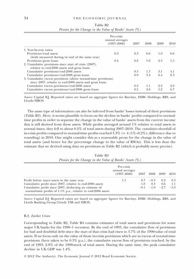
Table B2Proxies for the Change in the Value of Banks’ Assets (%)

Pre-crisisannual averages

(1997–2006) 2007 2008 2009 2010

1. Year-by-year ratiosProvisions ⁄ total assets

(both measured during ⁄ at end of the same year)0.3 0.3 0.6 1.0 0.6

Provisions ⁄ gross loans 0.4 0.8 1.6 2.3 1.52. Cumulative provisions since start of crisis (2007),

relative to end-2006 assets and gross loansCumulative provisions ⁄ end-2006 assets 0.5 1.7 3.1 4.1Cumulative provisions ⁄ end-2006 gross loans 0.9 3.4 6.4 8.3

3. Cumulative excess provisions (above normal-time provisions)since 2007, relative to end-2006 assets and gross loans

Cumulative excess provisions ⁄ end-2006 assets 0.2 1.1 2.2 2.9Cumulative excess provisions ⁄ end-2006 gross loans 0.5 2.6 5.2 6.7

Source: Capital IQ. Reported ratios are based on aggregate figures for Barclays, HSBC Holdings, RBS, andLloyds ⁄ HBOS.

The same type of information can also be inferred from banks’ losses instead of their provisions(Table B3). Here, it seems plausible to focus on the decline in banks’ profits compared to normal-time profits in order to separate the change in the value of banks’ assets from the current incomethat is still derived from these assets. While profits averaged around 1% relative to total assets innormal times, they fell to about 0.2% of total assets during 2007–2010. The cumulative shortfall ofin-crisis profits compared to normal-time profits reached 3.3% ( 4 (1%–0.2%); difference due torounding) in 2010. One might consider this as a reasonable proxy for the change in the value oftotal assets (and hence for the percentage change in the value of RWAs). This is less than theestimate that we derived using data on provisions in Table B2 (which is probably more precise).

Table B3Proxies for the Change in the Value of Banks’ Assets (%)

Pre-crisisannual averages

(1997–2006) 2007 2008 2009 2010

Profit before taxes ⁄ assets in the same year 1.1 0.7 �0.3 0.2 0.3Cumulative profit since 2007, relative to end-2006 assets 1.0 0.3 0.6 1.1Cumulative profit since 2007, deducting an estimate ofnormal-time profits of 1.1% p.a., relative to end-2006 assets

�0.1 �1.9 �2.7 �3.3

Source: Capital IQ. Reported ratios are based on aggregate figures for Barclays, HSBC Holdings, RBS, andLloyds Banking Group ⁄ Lloyds TSB and HBOS.

B.2. Earlier Crises

Corresponding to Table B2, Table B4 contains estimates of total assets and provisions for somemajor UK banks for the 1990–1 recession. By the end of 1993, the cumulative flow of provisionsfor bad and doubtful debt since the start of that crisis had risen to 3.7% of the 1990-value of totalassets. If we focus only on the value of those in-crisis provisions which are in excess of normal-timeprovisions (here taken to be 0.3% p.a.), the cumulative excess flow of provisions reached, by theend of 1993, 2.8% of the 1990-stock of total assets. During the same time, the peak cumulativedecline in UK GDP was 1.4%.



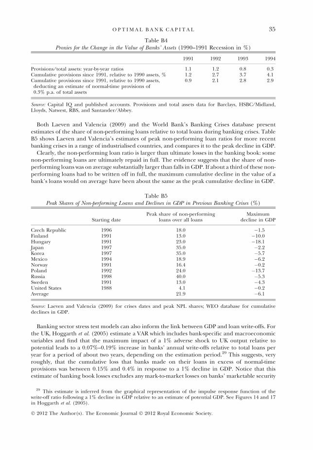
Table B4Proxies for the Change in the Value of Banks’ Assets (1990–1991 Recession in %)

1991 1992 1993 1994

Provisions ⁄ total assets: year-by-year ratios 1.1 1.2 0.8 0.3Cumulative provisions since 1991, relative to 1990 assets, % 1.2 2.7 3.7 4.1Cumulative provisions since 1991, relative to 1990 assets,deducting an estimate of normal-time provisions of0.3% p.a. of total assets

0.9 2.1 2.8 2.9

Source: Capital IQ and published accounts. Provisions and total assets data for Barclays, HSBC ⁄ Midland,Lloyds, Natwest, RBS, and Santander ⁄ Abbey.

Both Laeven and Valencia (2009) and the World Bank’s Banking Crises database presentestimates of the share of non-performing loans relative to total loans during banking crises. TableB5 shows Laeven and Valencia’s estimates of peak non-performing loan ratios for more recentbanking crises in a range of industrialised countries, and compares it to the peak decline in GDP.

Clearly, the non-performing loan ratio is larger than ultimate losses in the banking book: somenon-performing loans are ultimately repaid in full. The evidence suggests that the share of non-performing loans was on average substantially larger than falls in GDP. If about a third of these non-performing loans had to be written off in full, the maximum cumulative decline in the value of abank’s loans would on average have been about the same as the peak cumulative decline in GDP.

Table B5Peak Shares of Non-performing Loans and Declines in GDP in Previous Banking Crises (%)

Starting datePeak share of non-performing

loans over all loansMaximum

decline in GDP

Czech Republic 1996 18.0 �1.5Finland 1991 13.0 �10.0Hungary 1991 23.0 �18.1Japan 1997 35.0 �2.2Korea 1997 35.0 �5.7Mexico 1994 18.9 �6.2Norway 1991 16.4 �0.2Poland 1992 24.0 �13.7Russia 1998 40.0 �5.3Sweden 1991 13.0 �4.3United States 1988 4.1 �0.2Average 21.9 �6.1

Source: Laeven and Valencia (2009) for crises dates and peak NPL shares; WEO database for cumulativedeclines in GDP.

Banking sector stress test models can also inform the link between GDP and loan write-offs. Forthe UK, Hoggarth et al. (2005) estimate a VAR which includes bank-specific and macroeconomicvariables and find that the maximum impact of a 1% adverse shock to UK output relative topotential leads to a 0.07%–0.19% increase in banks’ annual write-offs relative to total loans peryear for a period of about two years, depending on the estimation period.29 This suggests, veryroughly, that the cumulative loss that banks made on their loans in excess of normal-timeprovisions was between 0.15% and 0.4% in response to a 1% decline in GDP. Notice that thisestimate of banking book losses excludes any mark-to-market losses on banks’ marketable security

29 This estimate is inferred from the graphical representation of the impulse response function of thewrite-off ratio following a 1% decline in GDP relative to an estimate of potential GDP. See Figures 14 and 17in Hoggarth et al. (2005).



holdings. It is also not clear what we should, for our purposes, infer from reaction functions thatare based on estimates derived from normal and crisis times; we are interested in protectingbanks from GDP fluctuations during crises.

We have recalculated optimal capital ratios assuming both less and more sensitivity of the fall inthe value of RWAs to a fall in GDP. The base case is a 1:1 percentage fall. Table B6 shows optimalcapital ratios when the fall in RWA is only ½ the percentage decline in GDP. Table B7 shows theimpact when the decline in the value of RWA is twice the percent decline in GDP. In both caseswe calculate optimal capital ignoring the most extreme bad events. Comparing the optimal ratiosin Tables B1 and B2 with those in Table 10 in the main text suggests that the impact on optimalbank capital of changing the assumed sensitivity of RWAs to falls in GDP is roughly linear.

Table B6Optimal Capital Ratios Ignoring the Most Extreme Bad Events – Half Sensitivity of RWA to GDP Fall

Crises have some permanenteffects on GDP growth (%)

Crises have no permanenteffects on GDP growth (%)

Base cost of capital 10 9Lower cost capital 10 10Higher cost capital 9 9

Table B7Optimal Capital Ratios Ignoring the Most Extreme Bad Events – Double Sensitivity of RWA to GDP Fall

Crises have some permanenteffects on GDP growth (%)

Crises have no permanenteffects on GDP growth (%)

Base cost of capital 35 32Lower cost capital 37 34

Monetary Policy Committee, Bank of EnglandBank for International SettlementsBank of England

Submitted: 14 April 2011Accepted: 23 December 2011

ReferencesAdmati, A., DeMarzo, P., Hellwig, M. and Pfleiderer, P. (2010). �Fallacies, irrelevant facts, and myths in capital

regulation: why bank equity is not expensive’. Stanford University Working Paper No. 86.Auerbach, A. (2002). �Taxation and corporate financial policy’, American Economic Review, Papers and Pro-

ceedings, vol. 92, pp. 67–178.Banerjee, A., Lumsdaine, R. and Stock, J. (1992). �Recursive and sequential tests of the unit-root and

trend-break hypotheses: theory and evidence’, Journal of Business & Economic Statistics, vol. 10, pp. 271–88.

Barnes, S., Price, S. and Barriel, M. (2008). �The elasticity of substitution: evidence from a UK firm-level dataset’, Bank of England Working Paper No. 348, April

Barrell, R., Davis, E., Fic, T., Holland, D., Kirby, S. and Liadze, I. (2009). �Optimal regulation of bank capitaland liquidity: how to calibrate new international standards’, FSA Occasional Paper 38.

Barro, R. (2006). �Rare disasters and asset markets in the twentieth century’, Quarterly Journal of Economics, vol.121(3), pp. 823–66.

BIS (2010a). �An assessment of the long-term economic impact of stronger capital and liquidity require-ments’, Basel Committee on Banking Supervision, Bank for International Settlements.



BIS (2010b). �Assessing the macroeconomic impact of the transition to stronger capital and liquidityrequirements’, Basel Committee on Banking Supervision, Bank for International Settlements.

BIS (2010c). �Results of the comprehensive quantitative impact study’, Basel Committee on Banking Supervision,Bank for International Settlements.

Calomiris, C. and Kahn, C. (1991). �The role of demandable debt in structuring optimal banking arrange-ments’, American Economic Review, vol. 81(3), pp. 497–513.

Campbell, J. and Mankiw, G. (1995). �Permanent and transitory components in macroeconomic fluctuations’,American Economic Review, vol. 77, pp. 111–7.

Cheng, Y. and Green, C. (2008). �Taxes and capital structure: a study of European companies’, The ManchesterSchool, vol. 76(S1), pp. 85–115.

Desai, A., Fritz Foley, C. and Hines, J. (2004). �A multinational perspective on capital structure choice andinternal capital markets’, Journal of Finance, vol. 59, pp. 2451–87.

Fleissig, A. and Strauss, J. (1999). �Is OECD real per capita GDP trend or difference stationary? Evidence frompanel unit root tests’, Journal of Macroeconomics, vol. 21(4), pp. 673–90.

Gertler, M., Kiyotaki, N. and Queralto, A. (2010). �Financial crises, bank risk exposure and governmentfinancial policy’, working paper, September. Available at: http://www2.lse.ac.uk/fmg/events/con-ferences/2010/financialIntermediation_Dec2010/financialIntermediation_KiyotakiPaper.pdf

Graham, J. (2003). �Taxes and corporate finance: a review’, Review of Financial Studies, vol. 16, pp. 1075–129.Haldane, A. (2010). �The $100 billion question’, Speech at the Institute of Regulation & Risk, North Asia

(IRRNA), Hong Kong. March.Hoggarth, G. and Pain, D. (2002). �Bank provisioning: the UK experience’, Bank of England Financial Stability

Review, June, pp. 116–27.Hoggarth, G., Sorensen, S. and Zicchino, L. (2005). �Stress tests of UK banks using a VAR approach’, Bank of

England Quarterly Bulletin, vol. 45(4), pp. 478.Homer, S. and Sylla, R. (1991). A History of Interest Rates, New Brunswick, NJ and London: Rutgers University

Press.Institute for International Finance (2010). Interim Report on the Cumulative Impact on the Global Economy of

Proposed Changes in Banking Regulatory Framework, Washington, DC: Institute for International Finance.Kashyap, K., Stein, J. and Hanson, S. (2010). �An analysis of the impact of ‘‘substantially heightened’’ capital

requirements on large financial institutions’, University of Chicago and Harvard Working Paper.Kay, J. (2009). Narrow Banking: The Reform of Banking Regulation, New York and London: Centre for the Study

of Financial Innovation.Kotlikoff, L. (2010). Jimmy Stuart is Dead: Ending the World’s Ongoing Financial Plague with Limited Purpose

Banking, Hoboken, NJ: John Wiley & Sons.Laeven, L. and Valencia, F. (2009). �Systemic banking crises: a new database’, IMF Working Paper No.

P ⁄ 08 ⁄ 224.Levin, A., Lin, C.-F. and Chu, C.-S.J. (2002). �Unit root tests in panel data: asymptotic and finite-sample

properties’, Journal of Econometrics, vol. 108, pp. 1–24.Macmillan (1931) �Report of the committee on finance and industry’, HM publications, Cmnd 3897.Miles, D., Pillonca, V. and Baker, M. (2005). �What should equities and bonds be worth in a risky world’,

Morgan Stanley Research Paper, September 2005.Miller, M. (1995). �Do the MM propositions apply to banks?’, Journal of Banking and Finance, vol. 19, pp. 483–9.Modigliani, F. and Miller, M. (1958). �The cost of capital, corporation finance and the theory of investment’,

American Economic Review, vol. 48(3), pp. 261–97.Nelson, C. and Plosser, C. (1982). �Trends and random walks in macroeconomic time series’, Journal of

Monetary Economics, vol. 10, pp. 139–62.Pandit, V. (2010). �We must rethink Basel, or growth will suffer’, Financial Times, 10 November.Perron, P. (1988). �Trends and random walks in macroeconomic time series: further evidence from a new

approach’, Journal of Macroeconomic Dynamics and Control, vol. 12, pp. 297–332.Radcliffe (1959). Report of the Committee on the Workings of the Monetary System, London: HM Publications, Cmnd.

827.Reinhart, C.M. and Rogoff, C. (2009). This Time is Different: Eight Centuries of Financial Folly, Princeton, NJ:

Princeton University Press.Smith, J. (2008). �That elusive elasticity and the ubiquitous bias: is panel data a panacea?’, Bank of England

Working Paper No. 342.Weichenrieder, A. and Klautke, T. (2008). �Taxes and the efficiency costs of capital distortions’, CESifo

Working Paper, No. 2431.Welch, I. (2001). �The equity premium consensus forecasts revisited’, Cowles Foundation, Discussion Paper

No. 1325.Wooldridge, J.M. (2002). Econometric Analysis of Cross Section and Panel Data, Cambridge, MA: MIT Press.



Optimal Bank Capital

Documents

Transcript of Optimal Bank Capital