Optimal allocation of wetlands: Study on conflict …gretha.u-bordeaux.fr/sites/default/files/WP...
22
GRETHA UMR CNRS 5113 Université Montesquieu Bordeaux IV Avenue Léon Duguit - 33608 PESSAC - FRANCE Tel : +33 (0)5.56.84.25.75 - Fax : +33 (0)5.56.84.86.47 - www.gretha.fr Optimal allocation of wetlands: Study on conflict between agriculture and fishery Natacha LASKOWSKI GREThA, CNRS, UMR 5113 Université de Bordeaux Cahiers du GREThA n° 2013-07 February
Transcript of Optimal allocation of wetlands: Study on conflict …gretha.u-bordeaux.fr/sites/default/files/WP...

GRETHA UMR CNRS 5113
Univers ité Montesquieu Bordeaux IV Avenue Léon Duguit - 33608 PESSAC - FRANCE
Tel : +33 (0)5.56.84.25.75 - Fax : +33 (0)5.56.84.86.47 - www.gretha.fr
Optimal allocation of wetlands: Study on conflict between agriculture and fishery
Natacha LASKOWSKI
GREThA, CNRS, UMR 5113
Université de Bordeaux
Cahiers du GREThA
n° 2013-07
February

Cahiers du GREThA 2013 – 01
GRETHA UMR CNRS 5113
Univers i té Montesquieu Bordeaux IV Avenue Léon Dugui t - 33608 PESSAC - FRANCE
Te l : +33 (0 )5 .56 .84.25 .75 - Fax : +33 (0 )5 .56 .84.86 .47 - www.gretha.f r
Allocation optimale d'une zone humide :
Etude du conflit d'usage entre agriculture et pêcherie
Résumé
Le modèle que nous développons s'intéresse à la question du conflit d'usage sur une zone humide exploitée par l'activité agricole et la pêcherie. A travers la modification de la fonction de croissance logistique et l'introduction de l'activité agricole dans les modèles traditionnels de pêcherie, nous nous intéressons à la taille optimale de la zone humide. Celle-ci sera fonction des profits des agents exploitants les ressources piscicoles d'une part, et les ressources agricoles d'autre part. L'étude statique puis dynamique de ce modèle permettra de tirer des enseignements sur le partage optimal des zones humides puis pourra servir de base l'élaboration de politiques de préservation des ressources.
Mots-clés : Zones humides, optimisation dynamique, capacité de charge, agriculture,
pêcherie, conflit d'usage
Optimal allocation of wetlands:
Study on conflict between agriculture and fishery
Abstract
The model developed here addresses the question of wetland conflict between agricultural production and fishery. Using the modification of the logistic function of growth and the introduction of agricultural activity into traditional fishing models, we consider the optimum allocation of wetlands. This depends on the profits of agents exploiting the fishing resources on the one hand and the agricultural resources on the other. Static followed by dynamic analysis of the model enable us to determine how best to allocate the use of wetlands, and then subsequently using that as a basis for developing sustainable conservation policies for resources
Keywords: Wetlands, dynamic optimisation, carrying capacity, agriculture, fishery, conflict
JEL: Q15, R52
Reference to this paper: LASKOWSKI Natacha (2013) Optimal allocation of wetlands: Study on
conflict between agriculture and fishery, Cahiers du GREThA, n°2013-07.
http://ideas.repec.org/p/grt/wpegrt/2013-07.html.

Introduction
Wetlands constitute some of the most vital environmental resources on our planet .
Once deemed unproductive, many of them have been converted to satisfy the needs
of agriculture for both water and land (Mitsch and Gosselink, 2000). Our insu�cient
understanding of wetlands and of their ecological and economic importance has led to
their being neglected, so that today it has now become urgent to protect and restore
them (Costanza et al., 1989 ; Costanza et al., 1998 ; Mitsch et Gosselink, 2000; de Groot,
Wilson and Boumans, 2002).
Ensuring their preservation is, however, a�ected by the underlying question of use
con�ict, when di�erent forms of activity are in competition within the boundaries of a
single site. This question of use con�ict has already been studied extensively. Bouba-
Olga et al. (2008) suggest addressing it as an issue of social competition concerning the
use of an environmental resource, or as a question of negative externalities which have
to be internalised. Cases of con�ict between aquaculture and �shery have been studied
by Hoagland, Jin and Kite-Powell (2003) and also by Mikkelsen (2007), who highlight
the competition that exists for the use of the area and its biological resources. Their
research attempted to resolve the question of the optimum amount of space required
by each activity within a given wetland area, by using simulations and modi�cations
of the parameters logistic function. This led to fresh light being shed on the negative
externalities that aquaculture can trigger for wild species and their farming.
These case studies, on which our approach is based, address the question of con�ict
between aquaculture and �shery. Here, however, we consider con�ict between �shery and
agriculture. Consequently, we do not study con�ict in terms of resources, but examine
con�ict focused on space, and its use for two di�erent activities. We explore these issues
via the pro�t functions of two agents, a farmer and a �sherman, considering the �sh
species from a biological angle. Using the logistic function of growth enables biological
parameters relating to resources to be integrated, thereby allowing us to examine the
question of con�ict in terms of the sustainability of the species in question.
This research lies at the crossroads of two main bodies of literature. On the one hand,
we examine use con�ict based on the case studies of �sh farming con�icts examined by
Hoagland, Jin and Kite-Powell (2003) and Mikkelsen (2007), but analysed here from
the perspective of the con�ict between �shery and agriculture by means of static and
dynamic modelling. Our static approach di�ers only marginally from that adopted
in the preceding research, even if the parameters it addresses are not the same. Our
dynamic modelling, however, innovates by allowing us to study the evolution of the
variables identi�ed and thus to de�ne an optimum allocation of wetlands between the
two competing commercial activities in place. In addition, from the perspective of
3
formalisation, our research develops and enriches that carried out by Barbier (2000;
2003), which stresses the consequences of a reduction in wetlands surface on the optimum
amount of �sh harvested. Barbier sheds light on the relation that exists between the size
of the zone in which �sh species live and the stock levels of each species. He concludes
that zone size reduction exercises a negative impact on the species. We reach similar
conclusions, in what concerns the link between agricultural activity and �shery, via the
notion of the area's carrying capacity.
The importance of this research is related to its impact in the �eld of policy mak-
ing, as the analysis of each agent's pro�ts and the optimum size of each agents zone,
along with the formulation of a shadow price, could be used to calculate a tax in order
to internalise externalities. The arbitrations highlighted here could then prove useful
for concrete applications, enabling policy makers to establish rules for dividing up the
available space, reconciling each agent's pro�ts with the biological sustainability of the
species. These elements will be examined from a static perspective in Section II, and
then from a dynamic perspective in Section III. Conclusions are then proposed concern-
ing the practical applications of this analysis for environmental policy making.
1 A Static Approach to Economic Modelling of the
Allocation of Wetlands
Our study of the con�ict between the area of the zone available for �shery and agricul-
tural activity is based on the logistic function of growth outlined by Verhulst (1838) and
on the models of Schaefer (1954) and Gordon-Schaefer (1954).
Let us consider wetlands in which agricultural activity occupies a part of the available
space, α (0 ≤ α < 1). The wetlands have a �xed surface area of S. Agriculture therefore
occupies a space which may be expressed as αS , in which S = γK. γ is a positive, �xed
parameter of spatialisation dependent on the characteristics of the natural environment.
K is the carrying capacity of that natural environment. The remaining area (1 - α)
is presumed to be non-anthropised and functioning in its original state. We suppose
the presence of �sh species and an ensuing commercial �shing activity, but without any
agricultural activity. When, however, the two activities are present, the question of
con�icting surface usage arises.
Agriculture, depending on the area it occupies, has a direct impact on wetlands.
We do not consider here any other direct or indirect e�ects, such as pollution of the
land or waterways due to the use of fertilisers or pesticides. Any increase in the total
area occupied by agricultural activity causes clear changes to the nature of the land
itself, making wetlands dry up, thereby reducing the area available for �sh species. We
4

suppose that the relationship between area and �sh production is linear.
Wetland con�ict arises from the fact that a single asset must be shared between
di�erent parties - on the one hand, the land may be exploited in the form of agri-
cultural production and, on the other, the water may be used for �sh farming. This
type of con�ict raises problems, which have not often been studied that of sharing the
same physical area but not the same resource, unlike more typical forms of competition
between di�erent agents for a single resource, as seen in �shery, for instance.
If we apply Verhulst's model of logistic growth, the logistic function expresses the
growth function of the �sh stock x as a function of the intrinsic growth rate r of the
population (r > 0) and the carrying capacity of the natural environment K (K > 0).
Given the negative impact of extension of the agricultural zone on the carrying capacity
of the natural environment, we replace K by K (1 - α) in the logistic growth function.
The logistic function now integrates the presence of agricultural activity in wetlands:
F (x) = rx
(1− x
K(1− α)
)(1)
The intrinsic growth rate of the population r coupled with the environmental resis-
tance factor(1− x
K(1−α)
)indicates the growth rate of the population.As the population
grows in its natural environment, con�ned by K(1−α), F(x) approaches 0. Conversely,
the smaller the �sh stock, the more population growth approaches r. Intuitively, we
understand that the more α approaches 1, the more the �sh population growth func-
tion approaches 0. Thus, if α is close to 1, this implies strong agricultural presence in
wetlands, triggering a fall in the �sh population and impoverishment of the wetlands.
Once the biological equilibrium of the resource at hand had been determined, we
studied the harvest function h de�ned by Schaefer (1954):
h = qEx (2)
with E representing the �shing e�ort mobilised and q the �shing e�ciency. The
�shing e�ort in relation to time t, depends on the number of boats deployed, the crew
size, number of days spent at sea, etc. The catchability q in relation to time t depends on
the given species (some being more di�cult to catch than others). The use of Schaefer's
harvest function posits that catch per unit of e�ort hE is proportional to �sh stock size,
for every level of stock and every level of �shing e�ort, thus presupposing that the
�sh population is evenly distributed throughout its natural habitat (Clark, 1990). The
predatory species here is the �sherman, whose harvest rate is directly linked to �shing
e�ort E, which allows this model to be used to analyse the paired evolution of the �shing
sector and the �sh population from a dynamic perspective and within a context in which
5

the two are inter-dependent. We suppose a reasonable �sh harvest, i.e h ≤ F (x). The
evolution of the �sh stock may then be expressed:
.x= rx(t)
(1− x(t)
K(1− α(t))
)− qE(t)x(t) (3)
At the point of biological equilibrium, the resource in steady state may be expressed
as:
F (x) = h(x) (4)
xSS(E) = K(1− α)(1− qE
r
)
The biological equilibrium of the resource xSS(E) in steady state, with modi�ed
carrying capacity, is lower than the point of equilibrium of the initial logistic function
xSSInitial(E) = (1 − qEr )K. Increased agricultural production, which raises the value of
the variable α, causes the level of the �sh stock in steady state to diminish, for a given
�shing e�ort.
Let us suppose a constant unitary cost of �shing e�ort c, and a constant price market
of the resrouce harvested p. The �sherman's pro�t may therefore be expressed as:
π(x,E) = pqEx− cE (5)
We have seen that the �sh population falls as the size of the agricultural area in-
creases. Given that(∂π∂x
), the �sherman's pro�t will necessarily fall in direct proportion
to the fall in �sh stock.
1.1 The open access situation
In the open access situation, the �sherman's return is equivalent to zero if we posit the
hypothesis of ownership of property rights by the farmer, and inversely if we posit that
all property rights are held by the �sherman. Economic equilibrium is de�ned by a
pro�t equivalent to zero. The Gordon-Schaefer (1954) model serves to analyse the long-
term consequences of �shing e�ort levels. It enables us to express the level of economic
equilibrium of the �shing sector. EOA is obtained by equalising total proceeds against
costs π = 0. This gives us:
EOA =r
q
(1− c
pqK(1− α)
)
EOA is an expression of �shing e�ort in the open access situation. We see that
6

∂EOA
∂α < 0 . This means that, as the area given over to agriculture increases, the �shing
e�ort decreases.
On the basis of biological and economic points of equilibrium, we may express the bio-
economic equilibrium of the resource as:
xOA = xSS(EOA) =c
pq(6)
The result of the Gordon-Schaefer model does not change, despite the introduction
of a variability parameter relative to carrying capacity. The �sh stock level in the open
access situation is not de�ned in relation to the area the �sh may colonise, but exclusively
in relation to the economic parameters and harvesting model. Indeed, xOA is a positive
function of �shing costs and a negative function of �sh prices and catchability. xOA
progression depends exclusively on its correlation with EOA, where these parameters
are �xed.
1.2 Individual optima and social optimum
Let us now look separately at the speci�c programmes of the �sherman and the farmer,
and then that of the social planner:
1.2.1 The Fisherman
The �sherman's aim is to maximise pro�t in relation to �shing e�ort and the amount
of �sh available. We will determine the optimal level of �shing e�ort and �sh stock. To
do so, we must maximise the function of the �sherman's pro�t:
maxE
π(xSS(E), E
)= pqK(1− α)
(1− qE
r
)E − cE (7)
We obtain
E∗ =r
2q
(1− c
pqK(1− α)
)x∗ =
1
2
((1− α)K +
c
pq
)π∗ =
r
4q
((pqK(1− α)− c)2
pqK(1− α)
)
For expressions E* and x*, we note that an increase in carrying capacity has a
positive e�ect on both �shing e�ort and �sh stock, and that conversely, over-present
agricultural activity weighs heavily onK and therefore also on E* and x*. The maximum
7
pro�t made by the �sherman decreases with α.
1.2.2 The Farmer
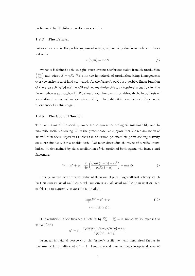
Let us now consider the pro�ts, expressed as ϕ(α,m), made by the farmer who cultivates
wetlands:
ϕ(α,m) = mαS (8)
wherem is de�ned as the margin or net revenue the farmer makes from his production(∂ϕ∂m
)and where S = γK. We pose the hypothesis of production being homogeneous
over the entire area of land cultivated. As the farmer's pro�t is a positive linear function
of the area cultivated αS, he will seek to maximise this area (optimal situation for the
farmer when α approaches 1). We should note, however, that although the hypothesis of
a variation in α on each occasion is certainly debateable, it is nonetheless indispensable
to our model at this stage.
1.2.3 The Social Planner
The main aims of the social planner are to guarantee ecological sustainability and to
maximise social well-being W. In the present case, we suppose that the maximisation of
W will ful�l these objectives in that the �sherman practices his pro�t-seeking activity
on a sustainable and reasonable basis. We must determine the value of α which max-
imises W, determined by the consolidation of the pro�ts of both agents, the farmer and
�sherman:
W = π∗ + ϕ =r
4q
((pqK(1− α)− c)2
pqK(1− α)
)+mαγS (9)
Finally, we will determine the value of the optimal part of agricultural activity which
best maximises social well-being. The maximisation of social well-being in relation to α
enables us to express this variable optimally:
maxα
W = π∗ + ϕ (10)
s.c. 0 ≤ α ≤ 1
The condition of the �rst order de�ned by ∂π∗
∂α + ∂ϕ∂α = 0 enables us to express the
value of α∗ :
α∗ = 1−2√mγr
(c√p− p
√Kcq
)+ cpr
Kpq(pr − 4mγ)
From an individual perspective, the farmer's pro�t has been maximised thanks to
the area of land cultivated α∗ = 1. From a social perspective, the optimal area of
8

agricultural land will increase or decrease in relation to varying parameters. A study
of the comparative statics allows us to advance a certain number of intuitive results.
We may observe, for example, that the optimal area of agricultural land cultivated is
correlated positively with the carrying capacity of the natural environment, just as it
is for price or catchability, and is negatively correlated with the cost of exploiting the
resource at hand and with the intrinsic growth rate of the stock.
∂(α∗)
∂K
∂(α∗)
∂c
∂(α∗)
∂r
∂(α∗)
∂p
∂(α∗)
∂q
∂(α∗)
∂γ
∂(α∗)
∂m
>0 <0 <0 >0 >0 >0 >0
Table 1: Comparative statics of parameters in α∗
Analysis of the optimal value of the proportion of agricultural land cultivated ?*
enables us to observe the progression of the pro�t made by the farmer in relation to
the progression of the land available for cultivation (Fig. 1). This shows how the pro�t
margin progresses and enables us to calculate the amount of compensation which a
farmer must receive if he is allow a given portion of his land to lie fallow, so that it
may be restored to its initial state as a wetland (from the perspective of a study of
compensation speci�cally designated for restoration projects). These results can help
pose the bases of e�cient environmental conservation policy making from the economic
point of view.
Figure 1: Progression of the farmer's pro�t margin in relation to area of agriculural land cultivated
(Source: author)
As the structure of this model is similar to that set out by Mikkelsen (2007), we may
also therefore apply his results and arrive at the following conclusion: if ∂W∂α > 0, ∀α,
then the wetlands are reserved for agricultural production alone and �shery cannot take
9

place due to the draining e�ect on the submerged areas of land. If ∂W∂α < 0, ∀α then
the wetlands have not been converted into usable farming land and �sh species may
therefore colonise them. These conclusions are valid if we accept the hypothesis that
we are exclusively considering the direct production function of �shery or agriculture.
In the present case, we do not attribute any value to the ecosystem or to the functions
it performs. If we do, however, take this into account, then we might suppose that
the signi�cance of the added environmental value of the wetland ecosystem would tip
the balance in favour of conservation of the zone, its speci�c functions and related
biodiversity.
2 Study of the Economic Model of the Allocation of
Wetlands from the Perspective of Dynamic Optimisa-
tion
2.1 Optimisation
Let us now address the problem from the dynamic perspective. The programme of the
social planner may be expressed as:
maxα(t),E(t)
∫ ∞0
(π(t) + ϕ(t)) e−ρtdt
s.c.
.x= rx(t)
(1− x(t)
K(1− α(t))
)− qE(t)x(t)
x0 = x(0)
where ρ is the discount rate. Our aim here is to maximise well-being in relation to
the constraints of resource dynamics and initial stock. The aim is to establish optimal
control involving two control variables - α(t) and E(t), and one state variable - x(t).
According to the Pontryagin Maximum Principle, the necessary condition which must
be ful�lled if control variables are to maximise the objective function, in light of the
constraints imposed, is that a variable λ(t) also exists which expresses the shadow price
of the resource. On the left side of the following Hamiltonian, we �nd the well-being
function studied in our static analysis, by specifying a quadratic function of the cost for
the �sherman. The current Hamiltonian is associated with the equation as:
H(E(t), x(t), α(t), λ(t), t) = pqE(t)x(t)− cE(t)2 +mγα(t)K
+ λ(t)
(rx(t)
(1− x(t)
K(1− α(t))
)− qE(t)x(t)
)(11)
10

2.2 First Order Conditions of the Hamiltonian
This Hamiltonian should reach its maximum at each moment t for the control and
state variables. In order to do so, the following First Order Conditions (FOC) must be
veri�ed:
FOC 1:
∂H(·)∂α(t)
= 0
Let:
ϕ′
α − λ(t)F′
α = 0 (12)
This enables us to determine the following expression of α(t) along the optimal trajec-
tory:
α(t) = 1− x(t)
K
√λ(t)r
mγ(13)
FOC 2:
∂H(·)∂E(t)
= 0
Let:
π′
E − λ(t)h′
E = 0 (14)
This enables us to determine the following expression of E(t) along the optimal trajec-
tory:
E(t) =qx(t)(p− λ(t))
2c(15)
FOC 3:
−∂H(·)∂x(t)
+ ρλ(t) =.
λ
Let:.
λ +π′
x = λ(t)(F′
x − h′
x + ρλ(t) (16)
This enables us to determine the following expression of λ(t) along the optimal trajec-
tory:.
λ= ρλ(t)− rx(t)(1− x(t)
K(1− α(t))
)− qE(t)x(t)) (17)
Equations 14 and 16 indicate the marginal conditions which the decision variables
must satisfy. The �rst equation indicates that the farmer's pro�t margin depends on
the marginal evolution of his resource and on the price at which the latter is evaluated.
Equation 16 expresses the fact that the �sherman's pro�t margin is equal to the harvest
function evaluated at its shadow price - each supplementary unit of pro�t made from
�shing is determined by each supplementary unit of resource harvested at the shadow
price. Equation 18 indicates how the adjoint variable progresses along its optimal tra-
11
jectory - the term on the left hand side represents the marginal increase in net price
and the marginal increase in the future pro�t then made by the �sherman. The term
on the right hand side represents the value of future harvesting of the resource and the
updated shadow price.
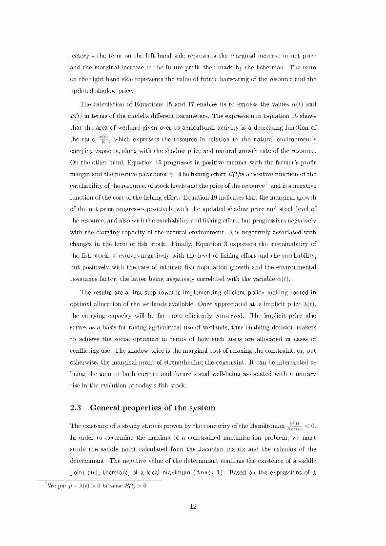
The calculation of Equations 15 and 17 enables us to express the values α(t) and
E(t) in terms of the model's di�erent parameters. The expression in Equation 15 shows
that the area of wetland given over to agricultural activity is a decreasing function of
the ratio x(t)K , which expresses the resource in relation to the natural environment's
carrying capacity, along with the shadow price and natural growth rate of the resource.
On the other hand, Equation 15 progresses in positive manner with the farmer's pro�t
margin and the positive parameter γ. The �shing e�ort E(t)is a positive function of the
catchability of the resource, of stock levels and the price of the resource 1 and is a negative
function of the cost of the �shing e�ort. Equation 19 indicates that the marginal growth
of the net price progresses positively with the updated shadow price and stock level of
the resource, and also with the catchability and �shing e�ort, but progressives negatively
with the carrying capacity of the natural environment..
λ is negatively associated with
changes in the level of �sh stock. Finally, Equation 3 expresses the sustainability of
the �sh stock..x evolves negatively with the level of �shing e�ort and the catchability,
but positively with the rate of intrinsic �sh population growth and the environmental
resistance factor, the latter being negatively correlated with the variable α(t).
The results are a �rst step towards implementing e�cient policy making rooted in
optimal allocation of the wetlands available. Once appreciated at is implicit price λ(t),
the carrying capacity will be far more e�ciently conserved. The implicit price also
serves as a basis for taxing agricultural use of wetlands, thus enabling decision makers
to achieve the social optimum in terms of how such areas are allocated in cases of
con�icting use. The shadow price is the marginal cost of relaxing the constraint, or, put
otherwise, the marginal pro�t of strengthening the constraint. It can be interpreted as
being the gain in both current and future social well-being associated with a unitary
rise in the evolution of today's �sh stock.
2.3 General properties of the system
The existence of a steady state is proven by the concavity of the Hamiltonian ∂2H∂x2(t) < 0.
In order to determine the maxima of a constrained maximisation problem, we must
study the saddle point calculated from the Jacobian matrix and the calculus of the
determinant. The negative value of the determinant con�rms the existence of a saddle
point and, therefore, of a local maximum (Annex 1). Based on the expressions of.
λ
1We put p− λ(t) > 0 because E(t) > 0
12
and.x determined by the formulations of FOC n 3 and Equation 3 respectively, we may
proceed to determine the values of.
λ and.x :
.
λ = ρλ− ∂H(·)∂x
= ρλ−(pqE + λ
(r − 2rx
K(1− α)− qE
)).x = ∂H(·)
∂λ = rx
(1− x
K(1− α)
)− qEx
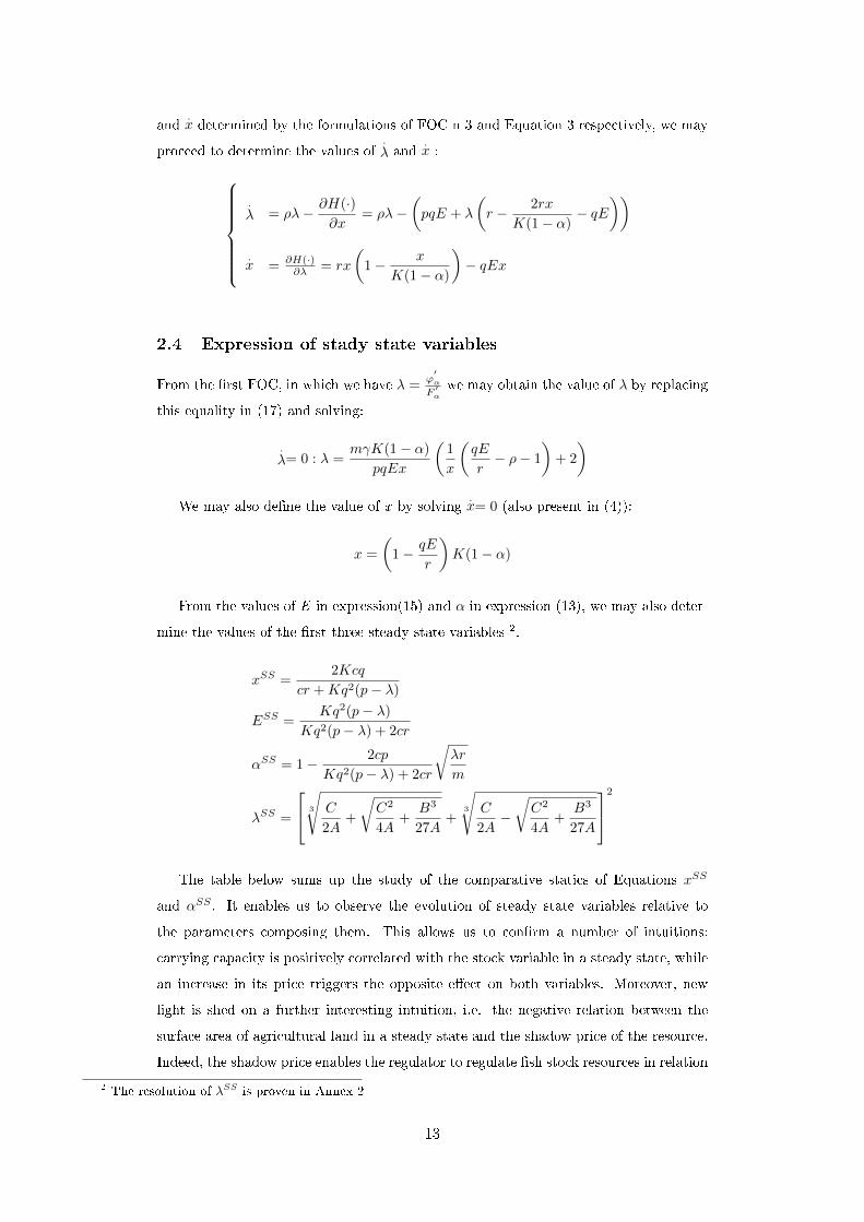
2.4 Expression of stady state variables
From the �rst FOC, in which we have λ =ϕ′α
F ′αwe may obtain the value of λ by replacing
this equality in (17) and solving:
.
λ= 0 : λ =mγK(1− α)
pqEx
(1
x
(qE
r− ρ− 1
)+ 2
)
We may also de�ne the value of x by solving.x= 0 (also present in (4)):
x =
(1− qE
r
)K(1− α)
From the values of E in expression(15) and α in expression (13), we may also deter-
mine the values of the �rst three steady state variables 2.
xSS =2Kcq
cr +Kq2(p− λ)
ESS =Kq2(p− λ)
Kq2(p− λ) + 2cr
αSS = 1− 2cp
Kq2(p− λ) + 2cr
√λr
m
λSS =
3
√C
2A+
√C2
4A+
B3
27A+
3
√C
2A−√C2
4A+
B3
27A
2
The table below sums up the study of the comparative statics of Equations xSS
and αSS . It enables us to observe the evolution of steady state variables relative to
the parameters composing them. This allows us to con�rm a number of intuitions:
carrying capacity is positively correlated with the stock variable in a steady state, while
an increase in its price triggers the opposite e�ect on both variables. Moreover, new
light is shed on a further interesting intuition, i.e. the negative relation between the
surface area of agricultural land in a steady state and the shadow price of the resource.
Indeed, the shadow price enables the regulator to regulate �sh stock resources in relation
2 The resolution of λSS is proven in Annex 2
13
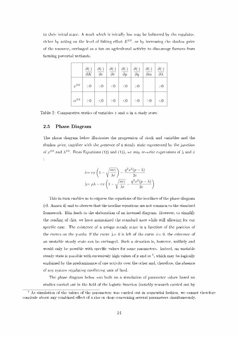
to their initial state. A stock which is initially low may be bolstered by the regulator,
either by acting on the level of �shing e�ort ESS , or by increasing the shadow price
of the resource, envisaged as a tax on agricultural activity to discourage farmers from
farming potential wetlands.
∂(·)∂K
∂(·)∂c
∂(·)∂r
∂(·)∂p
∂(·)∂q
∂(·)∂m
∂(·)∂λ
xSS >0 >0 <0 <0 >0 - >0
αSS >0 <0 >0 <0 >0 >0 <0
Table 2: Comparative statics of variables x and α in a stady state
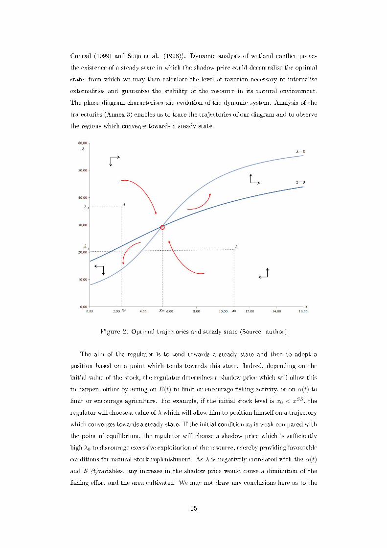
2.5 Phase Diagram
The phase diagram below illustrates the progression of stock and variables and the
shadow price, together with the presence of a steady state represented by the junction
of xSS and λSS . From Equations (13) and (15), we may re-write expressions of.
λ and.x
:
.x= rx
(1−
√mγ
λr
)− q2x2(p− λ)
2c
.
λ= ρλ− rx(1−
√mγ
λr− q2x2(p− λ)
2c
)
This in turn enables us to express the equations of the isoclines of the phase diagram
(cf. Annex 4) and to observe that the isocline equations are not common to the standard
framework. This leads to the elaboration of an inversed diagram. However, to simplify
the reading of this, we have maintained the standard axes while still allowing for our
speci�c case. The existence of a unique steady state is a function of the position of
the curves on the y-axis: if the curve.
λ= 0 is left of the curve.x= 0, the existence of
an unstable steady state can be envisaged. Such a situation is, however, unlikely and
would only be possible with speci�c values for some parameters. Indeed, an unstable
steady state is possible with excessively high values of p and m 3, which may be logically
explained by the predominance of one activity over the other and, therefore, the absence
of any system regulating con�icting uses of land.
The phase diagram below was built on a simulation of parameter values based on
studies carried out in the �eld of the logistic function (notably research carried out by
3 As simulation of the values of the parameters was carried out in sequential fashion, we cannot thereforeconclude about any combined e�ect of a rise or drop concerning several parameters simultaneously.
14
Conrad (1999) and Seijo et al. (1998)). Dynamic analysis of wetland con�ict proves
the existence of a steady state in which the shadow price could decentralise the optimal
state, from which we may then calculate the level of taxation necessary to internalise
externalities and guarantee the stability of the resource in its natural environment.
The phase diagram characterises the evolution of the dynamic system. Analysis of the
trajectories (Annex 3) enables us to trace the trajectories of our diagram and to observe
the regions which converge towards a steady state.
Figure 2: Optimal trajectories and steady state (Source: author)
The aim of the regulator is to tend towards a steady state and then to adopt a
position based on a point which tends towards this state. Indeed, depending on the
initial value of the stock, the regulator determines a shadow price which will allow this
to happen, either by acting on E(t) to limit or encourage �shing activity, or on α(t) to
limit or encourage agriculture. For example, if the initial stock level is x0 < xSS , the
regulator will choose a value of λ which will allow him to position himself on a trajectory
which converges towards a steady state. If the initial condition x0 is weak compared with
the point of equilibrium, the regulator will choose a shadow price which is su�ciently
high λ0 to discourage excessive exploitation of the resource, thereby providing favourable
conditions for natural stock replenishment. As λ is negatively correlated with the α(t)
and E (t)variables, any increase in the shadow price would cause a diminution of the
�shing e�ort and the area cultivated. We may not draw any conclusions here as to the
15

greater or lesser impact this might have on either activity. This would depend �rst and
foremost on the values of the parameters and the relative e�ciency of these commercial
activities.
If, however, the initial stock level is relatively high in comparison with the point of
equilibrium, x1 > xSS , then the regulator will aim at reducing the stock level. To do so,
he will choose a shadow price which is su�ciently weak λ1 to encourage either �shing
activity, through a variation in the �shing e�ort, or agricultural activity, through an
increase in the area of land available for cultivation. Therefore, depending on the initial
level of the stock, the regulator will determine a shadow price which will enable him
to position himself at A or B, thereby placing himself on a trajectory which converges
towards a steady state.
Conclusion
The main issue at stake in this research was to understand how best to allocate the use
of wetlands between competing commercial activities - �shing and agriculture. Although
our analysis of this question used previous research carried out by Barbier (2000 and
2003), Hoagland, Jin and Kite-Powell (2003) and Mikkelsen (2007), we have developed
and enriched their ideas by including a new element - agriculture - and a new method
- dynamic analysis. While the conclusions which may be drawn from our model are
subject to the supply and demand conditions of the market, the model, which accounts
for the biological elements of the species harvested, still remains highly original, thanks
to the logistic growth function. Indeed, the integration of this function adds a further
dimension to the model - that of sustainable development. The preservation or restora-
tion of wetlands can favour the development of numerous ecosystem goods and services,
notably in the �eld of �sh farming when it is managed on a sustainable basis.
The aim of this research was to study the impact of the reduction in surface area of
wetlands on �sh species and the ensuing economic consequences. In line with Barbier
(2000), our conclusions highlight the existence of a positive correlation between loss
of habitat and a decrease in the level of �sh stock. Arbitration and the de�nition
of an optimal size for each species is carried out with the economic interest of both
�shing and agricultural activity in mind. It would be possible to render this model
more complex in the future by integrating the question of contaminating substances
(pesticides, fertilizer?) used in agricultural production. To do so, we would need to
study in greater detail work carried out by Feunteun (2002) and Courrat et al. (2009)
dealing with the e�ect of polluting substances on �sh species in estuarine areas.
Finally, our paper is also relevant to the �eld of economic policies and is designed
16
to help decision making concerning the e�cient management of resources and highly
valuable ecological and economic zones. Our work would be useful in designing a tool
to encourage the restoration of wetlands thanks to the inclusion of a shadow price and
to the analysis of functions of pro�t margins of agents pro�ts.
References
Barbier, E.B., 1993. Sustainable use of wetlands valuing tropical wetland bene�ts: Eco-
nomic methodologies and applications. The Geographical Journal 159 (1), 22-32.
Barbier, E.B., 2000. Valuing the environment as input: Application to mangrove-
�shery linkages. Ecological Economics 35, 47-61.
Barbier, E.B., 2003. Habitat-�shery linkages and mangrove loss in Thailand. Con-
temporary Economic Policy 21 (1), 59-77.
Bouba-Olga, O., Boutry, O., Rivaud, A., 2008. Les con�its d'usage entre agriculture,
ostréiculture et plaisance sur le littoral Picto-Charentais. XLVème Colloque ASRDLF,
Territoire et action publique territoriale : nouvelles ressources pour le développement
régional, Québec.
Clark, C. W., 1990. Mathematical bioeconomics: The optimal management of re-
newable resources. Wiley-Intersciences, John Wiley & Sons, Second edition.
Conrad, J.M., 1999. Resource economics. Cambridge University Press, pp. 213.
Costanza, R., D'Arge, R., de Groot, R.S., Farber, S., Grasso, M., Hannon, B., Lim-
burg, K., Naeem, S., O'Neill, R., Paruelo, J., Raskin, R.G., Sutton, P., van den Belt,
M., 1997. The value of the world's ecosystem services and natural capital. Nature 387,
253-260.
Costanza, R., D'Arge, R., de Groot, R., Farber, S., Grasso, M., Hannon, B., Lim-
burg, K., Naeem, S., O'Neill, R.V., Paruelo, J., Raskin, R.G., Sutton, P., van den Belt,
M., 1998. The value of ecosystem services: Putting the issues in perspective. Ecological
Economics 25, 67-72.
Costanza, R., Farber, S.C., Maxwell, J., 1989. Valuation and management of wet-
land ecosystems. Ecological Economics 1, 335-361.
17

Courrat, A., Lobry, J., Nicolas, D., La�argue, P., Amara, R., Lepage, M., Girardin,
M., Le Pape, O., 2009. Anthropogenic disturbance on nursery function of estuarine
areas for marine species. Estuarine, Coastal and Shelf Science 81, 179-190.
Daily, G.C., 1997. Nature's services: Societal dependence on natural ecosystems.
Island Press, Washington.
De Groot, R.S., Wilson, M.A., Boumans, R.M.J., 2002. A typology for the classi�-
cation, description and valuation of ecosystem functions, goods and services. Ecological
Economics 41, 393-408.
Ferlin, P., 1986. Con�its et complémentarités entre les pêches côtières et l'aquaculture.
Report of the Technical Consultation of the General Fisheries Council for the Mediter-
ranean on the Methods of Evaluating Small-Scale Fisheries in the Western Mediter-
ranean, FAO Fishery Report N 362, 145-147.
Feunteun, E., 2002. Management and restoration of European eel population (An-
guilla anguilla): An impossible bargain. Ecological Engineering 18, 575-591.
Gren, I.-M., Folke, C., Turner, K., Bateman, I., 1994. Primary and secondary values
of wetland ecosystems. Environmental and Resource Economics 4, 55-74.
Hoagland, P., Jin, D., Powell-Kite, H., 2003. The optimal allocation of ocean space:
Aquaculture and wild-harvest �sheries. Marine Resource Economics 18, 29-47.
Kirat, T., Torre, A., 2004. Territoire, environnement et nouveaux modes de gestion
: La "gouvernance" en question. Modalités d'émergence et procédures de résolution des
con�its d'usage autour de l'espace et des ressources naturelles. Analyse dans les espaces
ruraux. Programme Environnement, Vie et Sociétés, Rapport de recherche, pp. 250.
Maltby, E., 1986. Waterlogged wealth: why waste the world's wet places?. Inter-
national Institute for Environment and Development, Earthscan Publications, London,
200 p.
May, R.M., 1981. Theoretical ecology. Oxford, UK: Blackwell Scienti�c Publica-
tions, Third Edition.
18

Mikkelsen, E., 2007. Aquaculture-�sheries interactions. Marine Resource Economics
22, 287-303.
Millennium Ecosystem Assessment, 2005. Ecosystems and human well-being: wet-
lands and water synthesis. Report, pp.80.
Mitsch, W.J., Gosselink, J.G., 2000. The value of wetlands: Importance of scale and
landscape setting. Ecological Economics 35, 25-33.
Seijo, J.C., Defeo, O., Salas, S., 1998. Fisheries bioeconomics. Theory, modelling
and management. FAO Fisheries Technical Paper. No.368. Rome, FAO, pp. 108.
Smardon, R.C., 2009. International wetland policy and management issues. In,
Sustaining the world's wetlands: Setting policy and resolving con�icts. Springer-Verlag
New York Inc., pp.17.
Annexes
Annex 1
Study of the sign of the determinant in the Jacobian matrix
.
λ = ρλ−(pqE + λ
(r − 2rx
K(1− α)− qE
))= 0
.x = rx
(1− x
K(1− α)
)− qEx = 0
J(x∗, λ∗) =
.xx (x∗, λ∗)
.xλ (x∗, λ∗)
.
λx (x∗, λ∗).
λλ (x∗, λ∗)
J(x∗, λ∗) =
< 0 = 0
> 0 > 0
⇒ detJ < 0
19
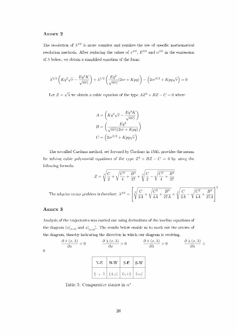
Annex 2
The resolution of λSS is more complex and requires the use of speci�c mathematical
resolution methods. After replacing the values of xSS , ESS and αSS in the expression
of λ below, we obtain a simpli�ed equation of the form:
λ3/2(Kq2√r − Eq4K
√mγ
)+ λ1/2
(Eq2√mγ
(2cr +Kpq)
)−(2cr3/2 +Kpq
√r)= 0
Let Z =√λ we obtain a cubic equation of the type AZ3 +BZ − C = 0 where
A =
(Kq2√r − Eq4K
√mγ
)B =
(Eq2
√mγ(2cr +Kpq)
)C =
(2cr3/2 +Kpq
√r)
The so-called Cardano method, set forward by Cardano in 1545, provides the means
for solving cubic polynomial equations of the type Z3 + BZ − C = 0 by using the
following formula:
Z =3
√C
2+
√C2
4+B3
27+
3
√C
2−√C2
4+B3
27
The solution to our problem is therefore: λSS =
3
√C
2A+
√C2
4A+
B3
27A+
3
√C
2A−√C2
4A+
B3
27A
2
Annex 3
Analysis of the trajectories was carried out using derivations of the isocline equations of
the diagram (x| .x=0 and x| .
λ=0). The results below enable us to mark out the arrows of
the diagram, thereby indicating the direction in which our diagram is evolving.
∂.x (x, λ)
∂x< 0
∂.
λ (x, λ)
∂x> 0
∂.x (x, λ)
∂λ> 0
∂.
λ (x, λ)
∂λ<
0
N-E N-W S-E S-W
(+,+) (+,-) (-,+) (-,-)
Table 3: Comparative statics in α∗
20

Annex 4
The equations of the isoclines in the phase diagram are as follows:
x| .x=0 =r(1−A)
B
x| .λ=0
=
(1−A)3B
3
√√√√√√√√√√√ A
9B3
(1−A+
A2
3− 1
3A
) +λ2ρ2
4B2r2− λρ
2Br
+3
√√√√√√√√√√√ A
9B3
(1−A+
A2
3− 1
3A
) +λ2ρ2
4B2r2− λρ
2Br
Where A =
√mγ
λrand B =
q2(p− λ)2c
, which enables us to re-write.
λ (x, λ) =
ρλ− rx(1−A−Bx2) and .x (x, λ) = rx(1−A)−Bx2.
21
Cahiers du GREThA
Working papers of GREThA
GREThA UMR CNRS 5113
Université Montesquieu Bordeaux IV
Avenue Léon Duguit
33608 PESSAC - FRANCE
Tel : +33 (0)5.56.84.25.75
Fax : +33 (0)5.56.84.86.47
http://gretha.u-bordeaux4.fr/
Cahiers du GREThA (derniers numéros – last issues)
2012-24 : LISSONI Francesco, MONTOBBIO Fabio, The ownership of academic patents and their impact. Evidence from five European countries
2012-25 : PETIT Emmanuel, TCHERKASSOF Anna, GASSMANN Xavier, Sincere Giving and Shame in a Dictator Game
2012-26 : LISSONI Francesco, PEZZONI Michele, POTI Bianca, ROMAGNOSI Sandra, University autonomy, IP legislation and academic patenting: Italy, 1996-2007
2012-27 : OUEDRAOGO Boukary, Population et environnement : Cas de la pression anthropique sur la forêt périurbaine de Gonsé au Burkina Faso.
2012-28 : OUEGRAOGO Boukary, FERRARI Sylvie, Incidence of forest income in reducing poverty and inequalities: Evidence from forest dependant households in managed forest’ areas in Burkina Faso
2012-29 : PEZZONI Michele, LISSONI Francesco, TARASCONI Gianluca, How To Kill Inventors: Testing The Massacrator
© Algorithm For Inventor Disambiguation
2013-01 : KAMMOUN Olfa, RAHMOUNI Mohieddine, Intellectual Property Rights, Appropriation Instruments and Innovation Activities: Evidence from Tunisian Firms
2013-02 : BLANCHETON Bertrand, NENOVSKY Nikolay, Protectionism and Protectionists Theories at the Balkans in the Interwar Period
2013-03 : AUGERAUD-VERON Emmanuelle, LEANDRI Marc, Optimal pollution control with distributed delays
2013-04 : MOUYSSET Lauriane, DOYEN Luc, PEREAU Jean-Christophe, JIGUET Frédéric, A double benefit of biodiversity in agriculture
2013-05 : OUEDRAOGO Boukary, HASSANE Mamoudou Co-intégration et causalité entre PIB, emploi et consommation d’énergie: évidence empirique sur les pays de l’UEMOA
2013-06 : MABROUK Fatma, À la recherche d’une typologie des migrants de retour : le cas des pays du Maghreb
2013-07 : LASKOWSKI Natacha, Optimal allocation of wetlands: Study on conflict between agriculture and fishery
La coordination scientifique des Cahiers du GREThA est assurée par Sylvie FERRARI et Vincent
FRIGANT. La mise en page est assurée par Anne-Laure MERLETTE.