Optimal acceptance sampling for modules F and F1 of the

European Measuring Instruments Directive

Cord A. Muller ∗

German Academy of Metrology (DAM),Bavarian State Office for Weights and Measures (LMG),Wittelsbacherstr. 17, 83435 Bad Reichenhall, Germany

March 29, 2019

Abstract

Acceptance sampling plans offered by ISO 2859-1 are far from optimal under the con-ditions for statistical verification in modules F and F1 as prescribed by Annex II of theMeasuring Instruments Directive (MID) 2014/32/EU, resulting in sample sizes that arelarger than necessary. An optimised single-sampling scheme is derived, both for large lotsusing the binomial distribution and for finite-sized lots using the exact hypergeometric dis-tribution, resulting in smaller sample sizes that are economically more efficient while offeringthe full statistical protection required by the MID.

Contents

1 Introduction 2

2 MID-optimised sampling plans for large lots 3

3 Finite lot sizes 63.1 Zero acceptance c = 0 . . . . . . . . . . . . . . . . . . . . . . . . . . . . . . . . . 63.2 Unit acceptance c = 1 . . . . . . . . . . . . . . . . . . . . . . . . . . . . . . . . . 103.3 Double acceptance c = 2 . . . . . . . . . . . . . . . . . . . . . . . . . . . . . . . 103.4 Summary of results for finite lot sizes . . . . . . . . . . . . . . . . . . . . . . . . . 12

4 Simplified single-sampling scheme 13

5 Outlook: alternative interpretation of the AQL criterion 16

A Interpretation of MID criteria for finite lots 16

∗cord.mueller@lmg.bayern.de

1

arX

iv:1

901.

0486

9v2

[st

at.A

P] 2

8 M

ar 2

019

1 Introduction

The European Measuring Instruments Direc-tive 2014/32/EU (MID) [1] states in Annex IIthat the statistical verification of products inmodules F and F1 must respect the followingconditions:

“The statistical control will be based on at-tributes. The sampling system shall ensure:

(a) a level of quality corresponding to a prob-ability of acceptance of 95%, with a non-conformity of less than 1%;

(b) a limit quality corresponding to a prob-ability of acceptance of 5%, with a non-conformity of less than 7%.”

These wordings must be cast into mathe-matical equations in order to determine accep-tance sampling plans to be used in practice,as described by the pioneering work of Dodgeand Romig [2]. There appears to be consensusamong the legal bodies in charge of administer-ing the tests [3] that the MID conditions shouldbe interpreted as

Pac(p) = 0.95 ⇒ p < 0.01, (1)

Pac(p) = 0.05 ⇒ p < 0.07. (2)

Here p is the quality level or “fraction defec-tive”, namely the fraction of non-conforming1

items in the lot, and Pac is the acceptanceprobability, a property of the statistical sam-pling plan to be devised. The first qualitylevel pa = 0.01 = 1% is commonly calledthe acceptance quality limit (AQL). The com-plement of the acceptance probability at thispoint, α = 1 − Pac(pa), is known as the pro-ducer’s risk that a lot with this acceptablelevel of quality is rejected. The second qualitylevel pb = 0.07 = 7% is known as the limitingquality (LQ), and the probability of acceptancePac(pb) = β is the consumer’s risk of acceptinga lot with this doubtful quality.

Since a lower quality level (i.e., larger p)should result in a lower acceptance probability,a valid function Pac(p) is strictly decreasing:

p > q ⇔ Pac(p) < Pac(q).2 Therefore, the two

conditions (1) and (2) for a certain samplingplan to be valid can be formulated equivalently

Pac(pa) < 0.95 = Pa, (3)

Pac(pb) < 0.05 = Pb. (4)

In other words, the MID conditions in the pre-vailing interpretation require

(a) a lot with AQL pa = 1% to imply a pro-ducer’s risk

α = 1− Pac(pa) > 5%, (5)

(b) and a lot with LQ pb = 7% to imply aconsumer’s risk

β = Pac(pb) < 5%. (6)

As a consequence, the graph of Pac(p), theso-called operating characteristic (OC), mustlie below and left of the two points MIDa =(pa, Pa) and MIDb = (pb, Pb). Figure 1shows, as an example, 3 OCs of different single-sampling plans for very large lots, based on thebinomial model of Section 2. Too small sam-ples are typically ruled out because their OCsviolate the MID conditions by lying above atleast one MID point, as illustrated by the planwith sample size n = 88 and acceptance num-ber c = 3. In contrast, large samples and largeacceptance numbers will typically result in OCsthat are far below the MID points; thus theyare certainly admissible. As an example, Fig. 1shows the OC of n = 800, c = 10, a mem-ber of the ISO 2859-1 family [4] that is recom-mended officially [3] for lot sizes from 150 001till 500 000. However, such a sampling is clearlybiased toward a much better quality level thanrequired by the MID conditions.

Sampling plans favouring very low AQLsare deemed admissible because the prevailinginterpretation of the MID conditions implies aproducer’s risk larger than 5% [Eq. (5)]. Themain point of the present work is that a sam-pling plan that is fair and economically accept-able for producers should not impose arbitraryconditions on the producers much stricter than

1We use the terms “non-conforming” and “defective” interchangeably for items that fail testing.2For finite lot sizes, Pac may not be strictly monotonic, but just monotonic. The MID conditions (1) and (2),

however, implicitly assume an infinite lot size; for details see Appendix A below.

2

0.00 0.01 0.02 0.03 0.04 0.05 0.06 0.07 0.08Level of quality p (fraction of non-conforming items)

0.0

0.1

0.2

0.3

0.4

0.5

0.6

0.7

0.8

0.9

1.0Ac

cept

ance

pro

babi

lity

P ac

MIDa = (pa, Pa)

MIDb

sampling plan (n, c):(88, 3): inadmissible(88, 2): optimal(800, 10): biased

Figure 1: Acceptance probability Pac as function of quality level p—the operating characteristic (OC)—of different single-sampling plans. An OC that does not lie below both points MIDa = (pa, Pa) =(0.01, 0.95) and MIDb = (pb, Pb) = (0.07, 0.05) is inadmissible according to the conditions (3) and (4).Optimal (unbiased) OCs are close to, and just below of, the two MID points. The three OCs shownare plotted using the binomial probability distribution [eq. (7)] for single sampling of n items with ac-ceptance number c. The plan (n = 88, c = 3) is inadmissible, (88, 2) is optimal, and (800, 10) is biasedtoward enforcing a much better quality level than required by the MID.

required by the MID, while respecting the le-gitimate interests of the consumers, of course.Therefore, MID-optimised sampling plans out-side the scope of ISO 2859-1 are derived inthe following sections, devoted to very largelots (Sec. 2) and finite-sized lots (Sec. 3), re-spectively. Readers not interested in details ofthe mathematical derivation are invited to skipto Sec. 4, where a simplified single-samplingscheme optimised for MID modules F and F1is proposed.

The concluding Sec. 5 finishes on the ob-servation that it would seem more reasonableif the sampling contract between producer andconsumer bounded both their risks from above,guaranteeing both β < 5% and α < 5%. Thisalternative interpretation of the MID’s AQLcondition has interesting consequences that are

briefly outlined, with details relegated to afollow-up paper.

2 MID-optimised samplingplans for large lots

In a first step, let us consider single samplingwhere n items are drawn from a very large lotwith a constant (but generally unknown) prob-ability p to be defective.3 The entire lot is ac-cepted if the number of defective items discov-ered by testing is not larger than the acceptancenumber c = 0, 1, 2, . . . . The acceptance prob-ability to find at most c defective items, eachfound independently from the others with iden-tical probability p, in a sample of size n is the

3Strictly, a probability 0 < p < 1 for a draw without replacement can only stay constant when the lot size Nis infinite; for now we assume N � n and consider corrections due to finite lot size in Sec. 3 below.

3

0.0

0.2

0.4

0.6

0.8

1.0

MIDa

MIDb

(42, 0)(50, 0)

(66, 1)(80, 1)

0.0

0.2

0.4

0.6

0.8

1.0(88, 2)(125, 2)

(138, 3)(200, 3)

0 1 2 3 4 5 6 7 80.0

0.2

0.4

0.6

0.8

1.0(199, 4)

0 1 2 3 4 5 6 7 8

(263, 5)(315, 5)

0.0 0.2 0.4 0.6 0.8 1.0Level of quality p[%] (percentage of non-conforming items)

0.0

0.2

0.4

0.6

0.8

1.0Ac

cept

ance

pro

babi

lity

P ac

Figure 2: Acceptance probability Pac(p, n, c) of various single-sampling plans (n, c) as function of qual-ity level p based on the binomial distribution Eq. (7). For each acceptance number c, the dashed curveshows the OC of the admissible standard ISO 2859-1 member [3], while the full curve shows the OC ofthe MID-minimised sample size. For small acceptance numbers c < 2, the LQ condition MIDb is themore stringent (OCs are not steep enough). For large acceptance numbers c > 2, the AQL conditionMIDa becomes more stringent (OCs are steeper than required). The optimal sample plan, defined bythe smallest sample size n while being unbiased with respect to both MID conditions, is (n, c) = (88, 2).

cumulative binomial distribution [5, 6]

Pac(p, n, c) =

c∑k=0

(n

k

)pk(1− p)n−k, (7)

where the binomial coefficient(nk

)= n!/[k!(n−

k)!] counts the number of different choices of kitems among n.

Figure 2 shows the resulting OCs for vari-ous single-sampling plans (n, c), grouped withincreasing acceptance number c = 0, 1, 2, . . .into pairs. The dashed curve shows the respec-tive member of the ISO 2859-1 family at in-

spection level II as recommended in [3].4 Thefull curve shows the smallest sample compatiblewith both MID conditions, which can be com-puted using standard numerical tools or com-mercial software, lowering the sample size un-til one of the two MID conditions is violated.Not surprisingly, when relaxing the constraintto the somewhat arbitrary members of the ISO2859-1 family, one obtains considerably smallersample sizes. Qualitatively, one arrives at thesame conclusion when approximating the bino-mial distribution (7) for p → 0, n → ∞ atfixed pn by the cumulative Poisson distribution

4For c = 4, ISO 2859-1 offers no sample size. Instead, it jumps directly from (200, 3) to (315, 5).

4

n c Pac(pa) α = 1−Pac(pa) qa β = Pac(pb) qb% % % % %

42 0 65.6 34.4 0.122 4.75 6.8850 0 60.5 39.5 0.103 2.66 5.8266 1 85.9 14.1 0.541 4.96 6.9980 1 80.9 19.1 0.446 2.11 5.7988 2 94.1 5.87 0.936 4.94 6.98125 2 86.9 13.1 0.657 0.62 4.95138 3 94.9 5.06 0.996 1.11 5.52200 3 85.8 14.2 0.686 0.03 3.83199 4 94.9 5.09 0.995 0.15 4.54

- 4 - - - - -263 5 95.0 5.04 0.998 0.02 3.96315 5 90.1 9.88 0.833 0.00 3.31

Table 1: Performance of the single-sampling plans (n, c) whose OCs are shown in Fig. 2. The producer’s(consumer’s) risk quality PRQ (CRQ) qa (qb) is the quality level where the allowed bound is reached,namely Pac(qa) = Pa = 95% (Pac(qb) = Pb = 5%). Gray-colored rows are the MID-optimised sampleplans, and white rows are the standard members of the ISO 2859-1 family; these offer no sample size forc = 4. Bold figures are close to, i.e., within 1% [0.1% for the PRQ qa] of the MID conditions. The leastbiased, minimal sample plan is (88,2).

Pac(p, n, c) ≈∑c

k=0 e−np(np)k/k!. Indeed, the

respective minimal sample sizes under the Pois-son approximation are, for c = 0, n = 43(+1),for c = 1, n = 68(+2), for c = 2, n = 90(+2),for c = 3, n = 137(−1), for c = 4, n = 198(−1),for c = 5, n = 262(−1), etc. Here, each num-ber in parentheses denotes the difference to theoptimal, and more accurate binomial result dis-played in the first two columns and grey-coloredrows of Table 1.

Because the probabilities for the differentcases k = 0, 1, 2, . . . , c in Eq. (7) add up andstill must stay below the MID points, the min-imum sample size grows with the acceptancenumber. In return, the OCs gain in specificity(smaller α) and sensitivity or statistical power(smaller β), i.e., permit to distinguish more ac-curately between high and low quality levels.For small acceptance numbers c = 0, 1, the LQcondition of MIDb is the more stringent, i.e.,OCs are not steep enough. For large acceptancenumbers c > 2, the AQL condition of MIDa

becomes more stringent, i.e., OCs are steeperthan required. The optimal sample plan, withsmallest sample size n while least biased withrespect to both MID conditions, is found to be(n, c) = (88, 2).

Table 1 lists the corresponding data, allow-ing for a quantitative comparison of the ISO2859-1 and MID-optimised sample plans. AsFig. 2 already shows, the LQ criterion MIDb

can be saturated quite well for low acceptancenumbers, with a consumer’s risk quality (CRQ)qb such that Pac(qb) = Pb not much belowpb = 7%, and a consumer’s risk β not muchbelow Pb = 5%. The price to be paid forsmall acceptance numbers and sample sizesis an elevated producer’s risk α, i.e., a highprobability for the type I error of rejecting agood lot. And the smallest admissible mem-ber (n, c) = (50, 0) of the ISO 2859-1 familyat inspection level II is stricter than necessarywith a producer’s risk of α = 39.5%; the cor-responding producer’s risk quality (PRQ) re-quired to reach Pac(qa) = Pa = 0.95 is aslow as qa = 0.103%. The minimal single-sampling plan (n, c) = (42, 0) compatible withMID conditions implies a slightly smaller pro-ducer’s risk α ≈ 34.4% with a slightly largerPRQ of qa = 0.122 and a CRQ qb just below7%.

Conversely, for larger acceptance numbersc ≥ 2 and, thus, larger sample sizes, the AQLcriterion MIDa becomes saturated with a pro-

5

ducer’s risk α approaching 5% from above.Here, the consumer’s risk drops to values β �1% much lower than required by MID, and aCRQ qb substantially smaller than 7%. Largersamples are indeed generally known to reducethe probabilities of type I and II errors andto have a greater discriminating power [5, 6].Thus, larger samples and higher acceptancenumbers have their merits in internal produc-tion control and may well be suggested in thecorresponding MID modules. However, a sys-tematic growth of sample size with lot size, asrecommended by the ISO 2859-1 sampling sys-tem, is not warranted by the MID conditionsfor modules F and F1.

In summary so far: For large enough lotsizes N � n (see Section 3.4 for a quantita-tive discussion) the minimal, least biased sam-ple plan for statistical product verification inthe MID modules F and F1 is (n, c) = (88, 2).

3 Finite lot sizes

If the lot size is not much larger than the sam-ple size then finite-size corrections become no-ticeable, and the results of the previous sectionhave to be revisited [5]. Let us consider a sam-ple of n items drawn without replacement froma lot of size N containing M ∈ {0, 1, . . . , N}defective items. Under the single-samplingparadigm, the lot is to be accepted if the samplecontains at most c defective items. The accep-tance probability is then given by the cumula-tive density of the hypergeometric distribution,

Pac(M,N, n, c) =

c∑k=0

(Mk

)(N−Mn−k

)(Nn

) , (8)

where each summand is the combinatorial prob-ability to find exactly k = 0, 1, . . . , c defectiveitems among the n items tested. One can assignthe quality level p = M/N to this lot and dis-cuss its acceptance probability Pac(pN,N, n, c)for fixed N as function of the operationallymeaningful values p ∈ DN , where

DN = {0, 1N ,

2N , . . . ,

N−1N , 1}. (9)

is the domain of the function Pac(·, N, n, c) :p ∈ DN 7→ Pac(p,N, n, c) ∈ Pac(DN ).

From this general setting follows

Proposition 1. A single-sampling plan withacceptance number c can only be admissible un-der the MID condition (3) for lot sizes

N > 100c. (10)

Proof. A lot containing at most M = c de-fective items will certainly be accepted by anysample plan (n, c). But then the correspond-ing quality level p = c

N (where Pac = 1) mustbe smaller than the AQL pa since otherwisecondition (3) cannot be satisfied. Therefore,cN < pa = 1

100 , which is equivalent to (10).

Analogously to the optimisation of samplesize in Section 2, one can further determine thesmallest sample size n, given acceptance num-ber c and lot size N > 100c, that is admis-sible under the MID conditions. We chooseto use the criteria (3) and (4), namely check-ing whether the acceptance probability (8) atMa = paN and Mb = pbN is inferior to thebounds Pa and Pb, respectively. This requiresthe extension of the factorials in (8) to non-integer arguments, which is easily achieved us-ing the gamma function [7]:

x! = Γ(x+ 1) =

∫ ∞0

txe−tdt. (11)

While the notion of non-integer values forMa =paN and Mb = pbN is not evident to justify op-erationally for single lots, this procedure turnsout to be more consistent than a purely discreteformulation; for a detailed justification see Ap-pendix A.

We find that the manner in which finitelot size affects MID-optimised sample plans de-pends crucially on the acceptance number. De-tails for the most relevant cases c = 0, 1, 2are discussed in the following subsections 3.1through 3.3. Readers mainly interested in thefinal results are invited to consult Sec. 3.4straight away.

3.1 Zero acceptance c = 0

For c = 0, the binomial prediction for very largelots (N = ∞) is conservative in the sense thatit overestimates the sample size that is really

6

0 1 2 3 4 5 6 7 8Level of quality p[%] (percentage of non-conforming items in a lot of size N)

0.0

0.1

0.2

0.3

0.4

0.5

0.6

0.7

0.8

0.9

1.0Ac

cept

ance

pro

babi

lity

P ac

MIDa

MIDb

(N, n, c) :(N = , 42, 0)(2048, 41, 0)(512, 40, 0)(256, 39, 0)(128, 36, 0)(64, 31, 0)(32, 24, 0)(16, 15, 0)

6 7 80.03

0.04

0.05

0.06

0.07

MIDb

Figure 3: Acceptance probability Pac(pN,N, n, 0) of minimal zero-acceptance single sampling plansadmissible under MID conditions, for lot sizes N following a geometric progression, plotted as functionof the lot’s quality level or fraction defective p = M/N . Filled colored dots correspond to the hyperge-ometric distribution (12); connecting curves are guides to the eye by the extension (11). The full blackline is the binomial sampling model for (n = 42, c = 0) reached in the limit N →∞.

necessary for a lot of a certain finite size N [5].Thus, (50, 0) from ISO 2859-1 has been cor-rectly identified as being compatible with MIDfor lot sizes from 51 ≤ N ≤ 500 [3]. Similarly,the single-sampling plan (42, 0) is certainly ad-missible, all the way down to N = 43. However,taking into account finite lot sizes allows us toreduce the required sample sizes even further.

Let us first explain qualitatively whysmaller lots require smaller zero-accceptancesamples. In the binomial model, the probabilityp to draw defective items without replacementfrom the lot is taken constant. However, if alot of size N contains M defective items, thenthe fraction defective is p = M/N only for thefirst draw. The probabilities of the second drawdepend on the outcome of the first. If the firstitem is defective, then the second item is de-fective with probability p′ = (M − 1)/(N − 1),which is smaller than p (we can assumeM < N ,since for M = N one has p = p′ = 1, a trivialcase without practical interest because all lots

are rejected anyway). Vice versa, if the firstitem is conforming, then p′ = M/(N−1), whichis larger than p (we assume M > 0, otherwisewe have p = p′ = 0, again a trivial case whereall lots are accepted). The latter case p′ > p ismore frequent since p � 1 in realistic settings.This evolution of the probability to larger val-ues will likely continue for each draw, so thatthe actual chance to discover defective items ina lot of small size is larger than predicted bythe binomial model. By consequence, the ac-tual acceptance probability for the same sam-ple size would be smaller, such that a smallersample actually suffices to stay below the MIDbounds.

For c = 0, the general expression (8) for theacceptance probability simplifies somewhat,

Pac(M,N, n, 0) =(N −M)!(N − n)!

N !(N −M − n)!. (12)

With the help of the factorial extension (11),one can determine numerically the smallest

7

10 20 50 100 200 500 1000 2000Lot size N (log scale)

15

20

25

30

35

40Sa

mpl

e siz

e n

(n N)

(32,24)

(64,31)

(128,36)

(256,39)(512,40)

(N = 16, n = 15)

(N = 2048, n = 41)

sample (n, c = 0):allowedminimal

Figure 4: MID-compatible sample size n for zero-acceptance single sampling as function of lot size N .For 1 ≤ N ≤ 15, only 100% testing n = N is admissible (see text). Between N = 16 and N = 3063, theminimum sample size grows slowly from n = 15 to n = 41, as listed in Table 2. From N ≥ 3064 onward,the mimimum sample size saturates at n = 42 already known from the binomial model (compare Fig. 2).Colored dots correspond to the OCs plotted in Fig. 3.

sample size n, given the lot size N , that stillfulfills both MID conditions. It turns out thatactually only the LQ condition (4) at MIDb

matters. Figure 3 shows the result of such aminimisation, for lot sizes N growing in geo-metric progression toward the limit N = ∞where the binomial result n = 42 of Section 2becomes exact. It is evident that sample sizescan be substantially reduced compared to thebinomial model for small to moderate lot sizes.

In theory, the smallest lot size for which sta-tistical sampling can be envisaged under theMID conditions is N = 15. The reason is thatfor 1 ≤ N ≤ 14, the quality level of a lot with asingle defective item is at least 1/14 ≈ 7.143%and thus already larger than pb = 7% thatshould be rejected. Therefore, the only wayto ensure MID conditions for N ≤ 14 is 100%testing with n = N . The next larger lot sizeN = 15 is such that a sample size of n = 14violates condition (4). Thus, also N = 15 re-

quires 100% testing with n = 15. The combi-nation N = 16 and n = 15, however, is com-patible with the MID conditions, as shown bythe corresponding OC in Fig. 3. For N = 17,one has to step up to n = 16, and so on, allthe way up to N = 3063 and n = 41. FromN ≥ 3064 onward, the required sample sizesaturates at n = 42 already derived from thebinomial model (cf. Fig. 2). Figure 4 shows theallowed and minimum sample size n found un-der MID conditions as function of the lot sizeN .

The corresponding lot-size intervals withtheir minimum sample sizes are listed in Ta-ble 2, together with the producer’s and con-sumer’s risks. Since the sample size is opti-mised with respect to the MID conditions (here,for c = 0, only the consumer’s point MIDb mat-ters), these data vary only slightly from onecase to the other. The main message is thatsample size can be substantially reduced, un-

8

Lot size N Sample Producer’s risk α [%] Consumer’s risk β [%]from to n c from to from to15 16 15 0 (40.37) (32.21) 0.00 4.1517 17 16 0 (34.53) (34.53) 3.00 3.0018 19 17 0 (36.82) (32.66) 2.13 4.4620 20 18 0 (34.73) (34.73) 3.42 3.4221 22 19 0 (36.77) (33.94) 2.61 4.0523 24 20 0 (35.84) (33.74) 3.19 4.31...

......

......

......

...56 61 30 0 (34.76) (33.70) 4.36 4.9462 69 31 0 (34.81) (33.66) 4.36 4.9970 78 32 0 (34.71) (33.71) 4.43 4.9979 89 33 0 (34.72) (33.77) 4.45 4.9890 103 34 0 (34.73) 33.81 4.47 4.97104 122 35 0 34.74 33.83 4.48 4.98123 148 36 0 34.71 33.85 4.51 4.99149 187 37 0 34.70 33.86 4.54 5.00188 248 38 0 34.66 33.89 4.57 5.00249 363 39 0 34.66 33.91 4.59 5.00364 659 40 0 34.65 33.93 4.61 5.00660 3063 41 0 34.63 33.95 4.63 5.003064 ∞ 42 0 34.62 34.4 4.65 4.75

Table 2: Minimum sample size n allowed by the MID for zero-acceptance single sampling as functionof lot size N , as shown in Fig. 4, together with the producer’s and consumer’s risk. Figures in paren-theses correspond to lot sizes N < 100, where a single defective item already defines a quality levelp = 1/N > pa such that the producer’s risk α = 1 − Pac(pa) has no operational meaning. Since thesample plans are optimised with respect to the MID conditions, the risk data stray only slightly fromthe values obtained in the limit N =∞, taken from the binomial model of Table 1. Entries “5.00” arisedue to rounding from the true values, which obey the strict inequality (4).

Lot size N Sample Producer’s risk α [%] Consumer’s risk β [%]from Na to Nb n c from to from to

139 142 55 1 5.07 5.26 4.88 4.98136 158 56 1 5.05 6.37 4.33 4.98133 178 57 1 5.02 7.41 3.83 4.99131 202 58 1 5.04 8.35 3.39 4.99129 234 59 1 5.05 9.26 2.98 4.99127 277 60 1 5.04 10.10 2.61 5.00125 337 61 1 5.00 10.88 2.27 5.00124 427 62 1 5.08 11.62 1.99 5.00123 581 63 1 5.14 12.31 1.74 5.00121 900 64 1 5.05 12.97 1.48 5.00120 1947 65 1 5.09 13.59 1.28 5.00119 ∞ 66 1 5.12 14.1 1.10 4.96

Table 3: Sample size n for unit-acceptance (c = 1) single sampling in the lot-size intervals [Na, Nb] al-lowed by MID, together with the producer’s and consumer’s risk. At Na, the producer’s risk is optimallyclose to (and just above) Pa = 5%; conversely, at Nb, the consumer’s risk is optimally close to (and justbelow) Pb = 5%. For N =∞ the data is taken from the binomial model (cf. Table 1).

9

200 500 1000 2000Lot size N (log scale)

50

52

54

56

58

60

62

64

66

68

70Sa

mpl

e siz

e n sample (n, c = 1):

allowedminimal, Naminimal, Nb

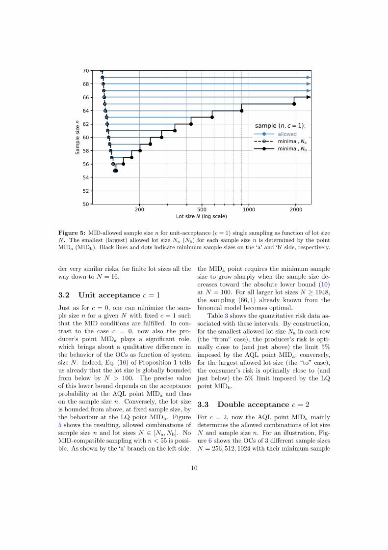
Figure 5: MID-allowed sample size n for unit-acceptance (c = 1) single sampling as function of lot sizeN . The smallest (largest) allowed lot size Na (Nb) for each sample size n is determined by the pointMIDa (MIDb). Black lines and dots indicate minimum sample sizes on the ‘a’ and ‘b’ side, respectively.

der very similar risks, for finite lot sizes all theway down to N = 16.

3.2 Unit acceptance c = 1

Just as for c = 0, one can minimize the sam-ple size n for a given N with fixed c = 1 suchthat the MID conditions are fulfilled. In con-trast to the case c = 0, now also the pro-ducer’s point MIDa plays a significant role,which brings about a qualitative difference inthe behavior of the OCs as function of systemsize N . Indeed, Eq. (10) of Proposition 1 tellsus already that the lot size is globally boundedfrom below by N > 100. The precise valueof this lower bound depends on the acceptanceprobability at the AQL point MIDa and thuson the sample size n. Conversely, the lot sizeis bounded from above, at fixed sample size, bythe behaviour at the LQ point MIDb. Figure5 shows the resulting, allowed combinations ofsample size n and lot sizes N ∈ [Na, Nb]. NoMID-compatible sampling with n < 55 is possi-ble. As shown by the ‘a’ branch on the left side,

the MIDa point requires the minimum samplesize to grow sharply when the sample size de-creases toward the absolute lower bound (10)at N = 100. For all larger lot sizes N ≥ 1948,the sampling (66, 1) already known from thebinomial model becomes optimal.

Table 3 shows the quantitative risk data as-sociated with these intervals. By construction,for the smallest allowed lot size Na in each row(the “from” case), the producer’s risk is opti-mally close to (and just above) the limit 5%imposed by the AQL point MIDa; conversely,for the largest allowed lot size (the “to” case),the consumer’s risk is optimally close to (andjust below) the 5% limit imposed by the LQpoint MIDb.

3.3 Double acceptance c = 2

For c = 2, now the AQL point MIDa mainlydetermines the allowed combinations of lot sizeN and sample size n. For an illustration, Fig-ure 6 shows the OCs of 3 different sample sizesN = 256, 512, 1024 with their minimum sample

10

0 1 2 3 4 5 6 7 8Level of quality p[%] (percentage of non-conforming items in a lot of size N)

0.0

0.1

0.2

0.3

0.4

0.5

0.6

0.7

0.8

0.9

1.0Ac

cept

ance

pro

babi

lity

P ac

MIDa

MIDb

(N, n, c) :(N = , 88, 2)(1024, 88, 2)(512, 95, 2)(256, 124, 2)

6.5 7.0 7.5 8.00.02

0.03

0.04

0.05

0.06

0.07

MIDb

0.8 1.0 1.20.90

0.95

1.00MIDa

Figure 6: Operating characteristics for lot sizes N = 256, 512, 1024 and their minimal double-acceptance(c = 2) single sampling plans under MID conditions. As shown in the inset on the lower left, now theAQL condition MIDa becomes increasingly hard to satisfy for smaller lots, such that the required samplesize has to increase quite dramatically. The exaggerated steepness of the OC curves for smaller lotsindicates that in those cases sampling with a lower acceptance number (c ≤ 1) is more appropriate.

sizes n = 124, 95, 88 determined by the MIDa

condition. Since the binomial limit (88, 2) isconservative in the sense that the acceptanceprobability (8) at pa increases as lot size N de-creases, then the minimum sample size has toincrease as well for smaller lots in order to com-pensate this effect. This one-sided constraintmakes the MIDb point increasingly irrelevant asN becomes smaller, as evident from the OC forthe smallest lot size N = 256 plotted in Fig. 6.The rapid decrease of the OC indicates thatthe acceptance number c = 2 is too elevatedfor such a small lot size, suggesting instead tofall back onto c = 1 or even c = 0.

Figure 7 shows the allowed combinations oflot and sample sizes. The minimum sample sizefound from the binomial model, n = 88, is ad-missble only down to N = 981. For smallerlots, the minimum sample size has to increasequite dramatically in order to satisfy the MIDa

condition. The MIDb constraint only has a

marginal influence: it limits the validity of thesmallest possible sample sizes n = 86, 87 toNb = 1469, 3412, respectively. The optimal bi-nomial result (n = 88, c = 2) is valid up toarbitrarily large lots, of course.

Table 4 lists the allowed sample size as func-tion of the lot size intervals, together with theproducer’s and consumer’s risks. It is clearthat for smaller lots, double-acceptance sam-pling is no longer the best choice for a fairrealization of the MID criteria. For example,a lot of size N = 256 requires the minimumdouble-acceptance sampling n = 124 and fea-tures only a consumer’s risk of β = 0.07%,two orders of magnitude smaller than requiredby MIDb. An arguably better choice then isc = 1, for which it can be found in Table 3 thatthe smallest allowed unit-acceptance sampling(60, 1) has α ≈ 10% and β ≈ 5%.

11

200 500 1000 2000 5000Lot size N (log scale)

80

90

100

110

120

130Sa

mpl

e siz

e n

(N = 1024, n = 88)

(N = 512, n = 95)

(N = 256, n = 124)

sample (n, c = 2):allowedminimal, Naminimal, Nb

Figure 7: MID-allowed sample size n for double-acceptance (c = 2) single sampling as function of lotsize N . The smallest (largest) allowed lot size Na (Nb) for each sample size n is determined by the pointMIDa (MIDb). Here the main factor is the MIDa condition, only the samples n = 86, 87 are limited tofinite lot sizes by the MIDb condition. The binomial result (88, 2) remains valid for arbitrarily large lots.The 3 colored dots correspond to the OCs plotted in Fig. 6.

3.4 Summary of results for finitelot sizes

Figure 8 summarizes the impact of finite lotsizes on the MID-optimised sampling schemewith acceptance number c = 0, 1, 2, coveringseveral orders of magnitude on a double loga-rithmic scale. The main results are:

1. The minimal sample plans (n, c) obtainedwithin the binomial model for large lotsin Sec. 2, (42, 0), (66, 1), and (88, 2), areindeed the minimal sample plans for alllot sizes N > Nc where N0 = 3063,N1 = 1947, and N2 = 3412. Finite-lot-size corrections are of two different types,dictated by the two different MID con-ditions. Their respective effects appeardepending on the acceptance number:

2. Acceptance number c = 0: The minimalbinomial sampling plan (42, 0) is conser-vative in the sense that it remains for-mally admissible down to N = 43. But

for lot sizes smaller than N0 = 3063,smaller samples are possible because itbecomes easier to satisfy the only relevantcondition (4) at LQ pb = 7%. The min-imum sample size as function of lot sizeis listed in Table 2 and shown in Figs. 4and 8.

3. Acceptance number c = 1: The minimalbinomial result (66, 1) is no longer glob-ally conservative. Certainly, below N1 =1947, the necessary sample size first de-creases for smaller lots because it becomeseasier to satisfy the LQ condition (4).But below a lot size of N = 139, wherethe smallest possible sample size is n =55, now the AQL condition MIDa takesover. It requires the sample size to growquite sharply with decreasing lot size inorder to ensure an acceptance probabilityat pa below 95%. This sharp upturn con-tinues down to N = 100, where the globallower bound (10) is reached. The admis-

12

Lot size N Sample Producer’s risk α [%] Consumer’s risk β [%]from Na to Nb n c from to from to

1454 1469 86 2 5.00 5.01 4.99 5.001166 3412 87 2 5.00 5.48 4.60 5.00981 ∞ 88 2 5.00 5.87 4.24 4.94852 ∞ 89 2 5.00 6.03 3.90 4.68757 ∞ 90 2 5.00 6.19 3.58 4.44684 ∞ 91 2 5.00 6.36 3.28 4.21626 ∞ 92 2 5.00 6.53 3.00 3.99579 ∞ 93 2 5.00 6.70 2.74 3.78540 ∞ 94 2 5.00 6.87 2.50 3.58508 ∞ 95 2 5.00 7.04 2.28 3.39480 ∞ 96 2 5.00 7.22 2.07 3.21

...257 ∞ 123 2 5.03 12.62 0.08 0.70254 ∞ 124 2 5.00 12.84 0.07 0.66252 ∞ 125 2 5.02 13.07 0.06 0.62

...

Table 4: MID-compatible lot and sample sizes for double-acceptance (c = 2) single sampling, togetherwith producer’s and consumer’s risk. The minimum sample size n = 88 found within the binomial modelis also the minimum sample size found here, valid for N ≥ 981. Smaller lots require larger samples. ForN < 500, the sample size rises substantially while the consumer’s risk drops far below the MID boundof 5%, indicating that unit-acceptance (c = 1) sampling is more appropriate.

sible (minimum) sample size as functionof lot size is listed in Table 3 and plottedin Fig. 5 (Fig. 8).

4. Acceptance number c = 2: The minimalbinomial result (88, 2) is not globally con-servative. Mainly the AQL condition (3)at MIDa is relevant, requiring the min-imum sample size to grow for decreas-ing lot size. This sharp upturn contin-ues down to N = 200, where the globallower bound (10) is reached. The admissi-ble (minimum) sample size as function oflot size is listed in Table 4 and plotted inFig. 7 (Fig. 8). Below roughly N = 500,the consumer’s risk drops far below theMID threshold such that c = 0, 1 accep-tance sampling becomes more appropri-ate.

5. Figure 8 also shows the ISO 2859-1 sam-pling plans recommended officially forMID modules F and F1 [3]. Clearly, theseare not minimal for low acceptance num-

bers c = 0, 1, 2. Moreover, their growthwith sample size, roughly as n ∼

√N ,

is not justified by the MID conditions asread in Sec. 1. By contrast, the MID-optimised sample plans derived here forc = 0, 1, 2 remain valid for arbitrarilylarge lots.

4 Simplified single-samplingscheme

The numerical minimisation of sample size asfunction of lot size under MID conditions pro-duces the sample plans (n, c) that are listed inTabs. 2, 3 and 4 for c = 0, 1, 2, respectively.Admittedly, these tables (and correspondingfigures) are more complicated than the sam-ple plans extracted from ISO 2859-1 that arerecommended hitherto [3]. It appears thereforeadvisable to condense the optimised plans intoa simplified sampling system that is still (al-most) optimal as far as the MID conditions are

13

101 102 103 104 105 106

Lot size N (log scale)

101

102

103

Min

imal

sam

ple

size

n (lo

g sc

ale)

(50, 0)

(125, 2)

(200, 3)

(315, 5)

(500, 7)

(800, 10)

(1250, 14)

(80, 1) (88, 2)(66, 1)

(42, 0)

(n N)

'MID ISO 2859-1'MID opt. c = 2MID opt. c = 1MID opt. c = 0

Figure 8: Combined view of MID-minimised single-sampling size n as function of lot size N for ac-ceptance numbers c = 0, 1, 2, together with the plans of ISO 2859-1 recommended by [3] (steps), on adouble-logarithmic scale.

Acceptance c = 0 Acceptance c = 1 Acceptance c = 2

Lot Sample Risk [%] Sample Risk [%] Sample Risk [%]

N n α ≤ β ≥ n α ≤ β ≥ n α ≤ β ≥21 to 24 20 (43.4) 0.69 - - - - - -

25 to 31 23 (44.6) 0.81 - - - - - -

32 to 41 26 (40.6) 1.90 - - - - - -

42 to 61 30 (40.5) 2.09 - - - - - -

62 to 122 35 (40.1) 2.30 - - - - - -

123 to 248 38 36.6 3.66 - - - - - -

249 to 500 40 35.4 4.21 63 12.2 3.77 - - -

501 to 1000 41 34.9 4.48 65 13.4 4.23 - - -

1001 to ∞ 42 35.0 4.44 66 14.1 4.45 88 5.87 4.25

Table 5: Proposal for a simplified single-sampling scheme optimised for MID modules F and F1 basedon the data of Tables 2, 3, and 4. In all cases, the producer’s risk is α > 5%, and the consumer’s risk isβ < 5%, as required by MID; here only the variable upper (lower) bound for α (β) is shown. For isolatedlots of size N < 100, the producer’s risk (listed in parentheses) has no operational significance becausethe AQL pa = 1% would correspond to less than a single defective item (M < 1).

14

101 102 103 104 105 106

Lot size N (log scale)

101

102

103

Sam

ple

size

n (lo

g sc

ale)

(50, 0)

(80, 1)

(125, 2)

(200, 3)

(315, 5)

(500, 7)

(800, 10)

(1250, 14)

(88, 2)(66, 1)

(42, 0)

(n N)

'MID ISO 2859-1'MID simpl. c = 2MID simpl. c = 1MID simpl. c = 0

Figure 9: Sample size as function of lot size for the simplefied, MID-optimised sampling scheme listedin Table 5, together with the single-sampling scheme from ISO 2859-1 [3], on a double-logarithmic scale.

concerned, but efficient to use in practice. Ta-ble 5 contains a proposal for such a samplingsystem, retaining the essential characteristicsof the MID-minimised sampling plans. Figure9 represents this simplified scheme, to be com-pared to the exact data represented in Fig. 8.The main steps taken to arrive at the simplifiedscheme are:

• choosing a simple lower bound N > 1000common to the relevant, minimal bino-mial sampling plans (42, 0), (66, 1), and(88, 2);

• binning lot sizes into a manageable num-ber of intervals common to all relevantacceptance numbers c = 0, 1, 2.

Such a simplified proposal is slightly arbitraryin the sense that one may as well choose differ-ent lot-size intervals with, consequently, a dif-ferent set of sample sizes. The present proposalaims at a reasonable compromise between the

complexity of the scheme and its logistic effi-ciency. Independently of the finer details, themain feature of our proposal is that the sam-ple size does not grow with the lot size aboveN = 1000, while offering the full statistical pro-tection required by the MID.

For small lot sizes N ≤ 248, only zero-acceptance sampling is found to be practical,with advantageously small samples but ratherelevated producer’s risks. The larger the lot,the more options are offered for statistical sam-pling. So one thing remains to be specified:Which acceptance number c = 0, 1 should bechosen above N = 248, and which of c = 0, 1, 2above N = 1000? Only if the producer knowsin advance that the quality level of the lot isperfect (p = 0 by production or strict exit con-trols), then c = 0 with the smallest possiblesample size is of course preferable. If the qual-ity level is finite (p > 0) but unkown, then thechoice of the sample plan is not uniquely deter-

15

mined by the MID conditions. Instead, the pro-ducer may decide which risk α is worth taking,depending on the lot’s known or expected qual-ity level, the production cost of each item, itsinspection cost, etc.. If, on the one hand, pro-duction costs are low, but inspection costs arehigh, then an elevated producer’s risk may beacceptable, and the smallest acceptance num-ber c = 0 is preferable with, consequently, thesmallest sample size. If, on the other hand, pro-duction costs are high and inspection costs arelow, then the producer’s risk can be substan-tially reduced by raising the acceptance num-ber to c = 2, together with an altogether mod-erate increase of sample size. In order to arriveat a truly (or at least approximately) optimalchoice, one would have to define an appropriatecost function and determine the optimal accep-tance number by an in-depth cost-benefit anal-ysis [8].

5 Outlook: alternative in-terpretation of the AQLcriterion

The AQL criterion of the MID, interpreted as inexpressions (1),(3), and (5), sets a lower boundon the producer’s risk. This is a somewhat cu-rious condition, already from an economic andcontractual point of view: why should the MIDguarantee a one-sided protection of the con-sumer’s interest at two points, without limit-ing the producer’s risk at the acceptance qual-ity level? Furthermore, this condition leadsto a number of awkward mathematical prop-erties that belie standard statistical knowledgein acceptance sampling. For example, the bino-mial approximation for the true hypergeomet-ric distribution is known to be conservative inthe sense that it provides larger samples thannecessary for a certain finite lot size [5]. Thisturns out not to be true here for c ≥ 1 samplingin the lot-size range where the AQL conditiondominates and requires larger samples than thebinomial approximation.

Indeed, standard textbooks formulate theAQL inequality usually the other way around,

setting an upper bound also on the producer’srisk—see, e.g., Eq. (10.57) in [6]. Additionally,an upper bound on both the consumer’s andproducer’s risk is compatible with the frame-work of hypothesis testing (see, e.g., section 2.2in [9]), which could have important conceptualand operational benefits [10]. Details of MID-optimised sampling plans obtained under suchan alternative interpretation of the MID’s AQLcriterion, however, are beyond the scope of thepresent work and will be presented in a forth-coming publication.

Acknowledgements

The author is indebted to Dr. Katy Klauenbergfor a critical reading of the manuscript and in-sightful comments.

A Interpretation of MIDcriteria for finite lots

We need to discuss the applicability of the MIDcriteria, either (1) and (2) or (3) and (4), forisolated lots of finite size, where quality lev-els and acceptance probabilities are discretesets. Consider a lot of size N , containing an(unknown) number M ∈ {0, 1, . . . , N} of non-conforming items. One can assign the qualitylevel p = M/N to this lot and discuss its accep-tance probability Pac(p) under a certain sam-pling plan as function of the meaningful values

p ∈ DN = {0, 1N ,

2N , . . . ,

N−1N , 1}. (13)

Now, the two special quality levels of the MIDconditions, pa = 1

100 and pb = 7100 , are only in

the domain DN if N is an integer multiple of100. For all other lot sizes, pi /∈ DN such thatPac(piN,N, n, c) as given by eq. (8) is not de-fined, at least not in simple operational termsrelated to the sampling of a single lot, where Mmust be an integer. As a consequence, the MIDconditions (3) and (4) cannot be applied as suchfor deciding whether a sampling plan is admis-sible or not. And even if per chance N is a mul-tiple of 100, also the image ofDN under Pac, the

16

0 10 20 30 40 50 60 70 80Lot size N

0

5

10

15

20

25

30

35

40Sa

mpl

e siz

e n

(n N)

min. sample size (c = 0):MIDb discreteMIDb continuous

Figure 10: Minimum sample size as function of lot size for zero-acceptance sampling (c = 0). Thepurely ‘discrete’ MID criteria (15) (blue diamonds) result in non-monotonic jumps, whereas the analyt-ical coninuation introduced in Sec. 3.1 (black circles) provides a non-decreasing, conservative bound forthe minimum sample size. Since c = 0, only the MIDb criterion is actually relevant (cf. Sec. 3.1).

set Pac(DN ) of the different acceptance proba-bilities, is now a discrete set that will generallynot contain the two values Pa = 95

100 = 1920 and

Pb = 5100 = 1

20 . In other words, in most casesthere will be no qi ∈ DN such that Pac(qi) = Pi,exactly. Thus, also the MID conditions (1) and(2) cannot be applied as such.

It thus becomes clear that the wording ofthe MID implicitly assumes a continuous de-scription, which applies only to process sam-pling with a formally infinite lot size (called“type B” in [5, 6]). However, the MID producttesting in modules F and F1 typically involvesisolated lots of finite size, where the continuityof type B testing cannot be taken for granted.In a first attempt to render the MID conditionsmeaningful for finite lot sizes, we have tried to

interpret the wording “corresponding to a prob-ability of acceptance of Pi” as meaning “corre-sponding to a probability of acceptance of atleast Pi”.5 Then, the two MID conditions (1)and (2) are rather

Pac(p) ≥ Pi ⇒ p < pi, i = a,b, (14)

which can be tested for all p ∈ DN . A log-ically equivalent, but more practical criterionthat can be readily evaluated with a computeris obtained by the negation of (14), namely

p ≥ pi ⇒ Pac(p) < Pi, i = a,b. (15)

Under these premises, in order to test the ad-missibility of a certain sampling plan, one onlyneeds to take the first allowed quality levels

5In the continuous case, this follows already from the monotonicity and continuity of Pac: There is exactly oneqi such that Pac(qi) = Pi and for which MID implies qi < pi. Now take any p such that Pac(p) > Pac(qi). Themonotonicity (p > qi ⇒ Pac(p) ≤ Pac(qi)) in its negated form Pac(p) > Pac(qi) ⇒ p ≤ qi then implies togetherwith qi < pi the r.h.s. p < pi. So the MID conditions could have been formulated with a “probability of at leastPi” from the start.

17

p ∈ DN larger than or equal to pa and pb, re-spectively, and check whether Pac(p) at thesepoints is smaller than Pa and Pb, respectively.If that is the case, then the plan is approved(monotonicity guarantees that even larger pcannot yield larger values of Pac), and if not,it is rejected.

While this interpretation is logically satis-fying and economical to evaluate, it leads toinconsistencies due to discretisation effects. In-deed, when the lot size is increased such thatone quality level pj ∈ DN drops below pb, thenext higher quality level pj+1 becomes relevantsuch that suddenly a smaller sample may be-come allowed. Figure 10 shows the c = 0 mini-mum sample size as function of lot size result-ing from the purely ‘discrete’ criterion (15). Itfeatures a prominent saw-tooth structure whereraising the lot size at certain points (e.g., fromN = 42 to 43) suddenly lowers the minimumsample size (e.g., from n = 26 to 22).

Such an erratic dependence of sample sizeon lot size is arguably not a desirable featureof an acceptance sampling plan. Therefore, wehave proposed in Sec. 3.1 to extend the accep-tance probabilities in the standard manner tonon-integer item numbers, formally adopting atype-B testing scenario that allows us to evalu-ate Pac(p) at pa and pb for any lot size and thusto use the MID criteria (3) and (4) just as ina truly continuous case. The advantage is two-fold: First, the resulting sample size is conser-vative, namely, never smaller than prescribedby the discrete criterion (15) at the consumer’sLQ point, where also the binomial model forinfinite lots is conservative. Second, the mini-mum lot size resulting from the consumer’s LQpoint condition is a non-decreasing function oflot size, as evident from Fig. 10 (see also Fig. 4and the relevant portion of Fig. 5).

References

[1] Directive 2014/32/EU of the European Par-liament and of the Council of 26 February

2014 on the harmonisation of the laws ofthe Member States relating to the makingavailable on the market of measuring instru-ments (recast), OJ L96/149 (2014)

[2] H F. Dodge, H. G. Romig, ”A Method ofSampling Inspection”, Bell Syst. Tech. J. 8,613-631, 1929

[3] WELMEC European cooperation in legalmetrology: Working group 8, Measuring In-struments Directive (2014/32/EU): Guidefor generating sampling plans for statisti-cal verification according to Annex F andF1 of MID 2014/32/EU (2018)

[4] ISO/TC 69/SC 5, ”Sampling procedures forinspection by attributes - Part 1: Samplingschemes indexed by acceptance quality limit(AQL) for lot-by-lot inspection”, ISO 2859-1:1999(E)

[5] E.G. Schilling, D. V. Neubauer, AcceptanceSampling in Quality Control (CRC Press,Boca Raton, 2017)

[6] P. Mathews, Sample Size Calculations.Practical Methods for Engineers and Scien-tists (Mathews Malnar and Bailey, FairportHarbor, 2010).

[7] M. Abramowitz and I. A. Stegun (eds.), TheHandbook of Mathematical Functions withFormulas, Graphs, and Mathematical Ta-bles National Bureau of Standards AppliedMathematics Series 55 (1972).

[8] H. F. Campbell and R. Brown, “Incorporat-ing Risk in Benefit-Cost Analysis”. Benefit-Cost Analysis: Financial and EconomicAppraisal using Spreadsheets (CambridgeUniversity Press, Cambridge, 2003)

[9] K. Klauenberg and C. Elster, ”Sampling forassurance of future reliability”, Metrologia54, 59 (2017)

[10] R.W. Samohyl, ”Acceptance sampling forattributes”, J. Ind. Eng. Int. 14, 395 (2018)

18