Moving theory to applications, 22-10, Palaiseau

Optical properties of SnO2

Arjan Berger

Laboratoire des Solides IrradiesEcole Polytechnique, Palaiseau, France

European Theoretical Spectroscopy Facility (ETSF)

Outline

I SnO2 facts

I Motivation

I Results

I Conclusions

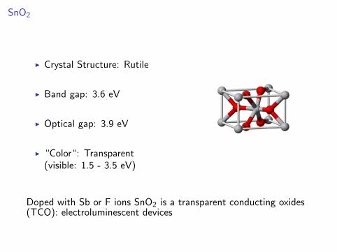
SnO2

I Crystal Structure: Rutile

I Band gap: 3.6 eV

I Optical gap: 3.9 eV

I “Color“: Transparent(visible: 1.5 - 3.5 eV)

Doped with Sb or F ions SnO2 is a transparent conducting oxides(TCO): electroluminescent devices

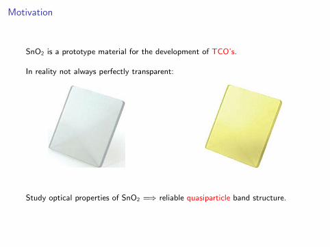
Motivation

SnO2 is a prototype material for the development of TCO’s.

In reality not always perfectly transparent:

Study optical properties of SnO2 =⇒ reliable quasiparticle band structure.

Motivation

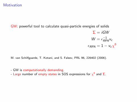
GW: powerful tool to calculate quasi-particle energies of solids

Σ = iGW

W = ε−1RPAvc

εRPA = 1− vcχ0

M. van Schilfgaarde, T. Kotani, and S. Faleev, PRL 96, 226402 (2006).

- GW is computationally demanding.- Large number of empty states in SOS expressions for χ0 and Σ.

The Polarizability

Standard calculation of χ0 and Σ: sum over states (SOS)

χ0GG′(q, ω) =

occ∑v

empty∑c

〈v |e−i(q+G)·r|c〉〈c|e i(q+G′)·r′ |v〉ω − (εc − εv ) + iη

+ A.R.

Advantages:

I Systematic and controllable

I Easy to implement

Disadvantages:

I Huge summation over empty states

I Slow (scaling=NcNvN2G)

Aim:- Keep advantages of SOS- Get rid of disadvantages: occupied states only

The Polarizability

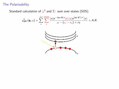
Standard calculation of χ0 and Σ: sum over states (SOS)

χ0GG′(q, ω) =

occ∑v

empty∑c

〈v |e−i(q+G)·r|c〉〈c|e i(q+G′)·r′ |v〉ω − (εc − εv ) + iη

+ A.R.

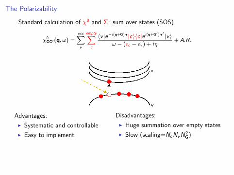
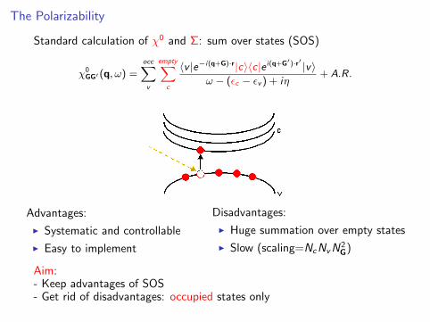
Advantages:

I Systematic and controllable

I Easy to implement

Disadvantages:

I Huge summation over empty states

I Slow (scaling=NcNvN2G)

Aim:- Keep advantages of SOS- Get rid of disadvantages: occupied states only

The Polarizability

Standard calculation of χ0 and Σ: sum over states (SOS)

χ0GG′(q, ω) =

occ∑v

empty∑c

〈v |e−i(q+G)·r|c〉〈c|e i(q+G′)·r′ |v〉ω − (εc − εv ) + iη

+ A.R.

Advantages:

I Systematic and controllable

I Easy to implement

Disadvantages:

I Huge summation over empty states

I Slow (scaling=NcNvN2G)

Aim:- Keep advantages of SOS- Get rid of disadvantages: occupied states only

Four Criteria for GW

I Systematic and controllable

I Easy to implement

I No summation over empty states

I Better scaling properties than SOS

Other GW approaches with less or no empty states:

COHSEX:

Extrapolar method:

Sternheimer equation:

L. Hedin, PR A796 (1965)

F. Bruneval and X. Gonze, PRB 78, 085125 (2008).

L. Reining et al., PRB 56, R4302 (1997)P. Umari et al., PRB 81 115104 (2010)F. Giustino et al., PRB 81 115105 (2010)

So far: no GW approach which satisfies all criteria simultaneously

Four Criteria for GW

I Systematic and controllable

I Easy to implement

I No summation over empty states

I Better scaling properties than SOS

Other GW approaches with less or no empty states:

COHSEX:

Extrapolar method:

Sternheimer equation:

L. Hedin, PR A796 (1965)

F. Bruneval and X. Gonze, PRB 78, 085125 (2008).

L. Reining et al., PRB 56, R4302 (1997)P. Umari et al., PRB 81 115104 (2010)F. Giustino et al., PRB 81 115105 (2010)

So far: no GW approach which satisfies all criteria simultaneously

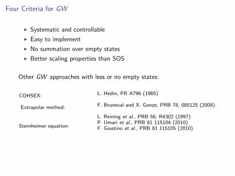
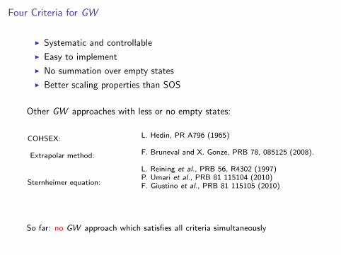
Four Criteria for GW

I Systematic and controllable

I Easy to implement

I No summation over empty states

I Better scaling properties than SOS

Other GW approaches with less or no empty states:

COHSEX:

Extrapolar method:

Sternheimer equation:

L. Hedin, PR A796 (1965)

F. Bruneval and X. Gonze, PRB 78, 085125 (2008).

L. Reining et al., PRB 56, R4302 (1997)P. Umari et al., PRB 81 115104 (2010)F. Giustino et al., PRB 81 115105 (2010)

So far: no GW approach which satisfies all criteria simultaneously

ΣGW with sum over occupied states only

The bottleneck in the calculation of ΣGW :

〈n|Σemptyc (ω)|n〉 =

∑q,G,G′

∑j

W jGG′(q)

empty∑c

〈n|e i(q+G)·r|c〉〈c|e−i(q+G′)·r′ |n〉ω − ωj − εc

There exists an effective energy δnj(q,G,G′, ω) such that

empty∑c

〈n|e i(q+G)·r|c〉〈c|e−i(q+G′)·r′ |n〉ω − ωj − εc

=〈n|e i(q+G)·r (∑empty

c |c〉〈c|)e−i(q+G′)·r′ |n〉

ω − ωj − δnj(q,G,G′, ω)

Closure relation:∑empty

c |c〉〈c | = 1−∑occ

v |v〉〈v |

=⇒

EET: Effective Energy Technique

ΣGW with sum over occupied states only

The bottleneck in the calculation of ΣGW :

〈n|Σemptyc (ω)|n〉 =

∑q,G,G′

∑j

W jGG′(q)

empty∑c

〈n|e i(q+G)·r|c〉〈c|e−i(q+G′)·r′ |n〉ω − ωj − εc

There exists an effective energy δnj(q,G,G′, ω) such that

empty∑c

〈n|e i(q+G)·r|c〉〈c|e−i(q+G′)·r′ |n〉ω − ωj − εc

=〈n|e i(q+G)·r (∑empty

c |c〉〈c|)e−i(q+G′)·r′ |n〉

ω − ωj − δnj(q,G,G′, ω)

Closure relation:∑empty

c |c〉〈c | = 1−∑occ

v |v〉〈v |

=⇒

EET: Effective Energy Technique

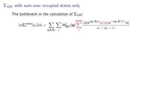
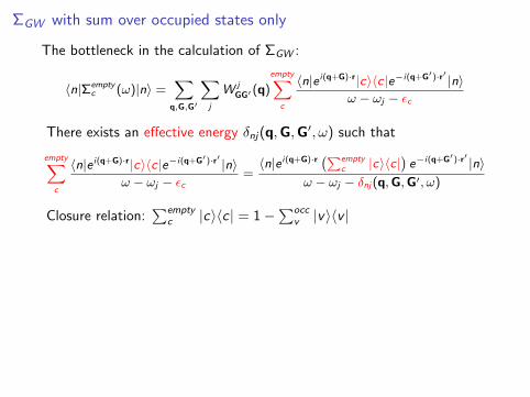
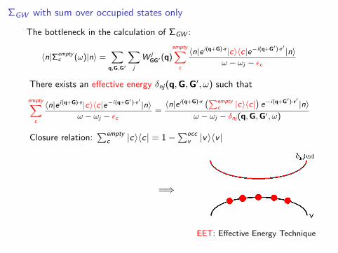
ΣGW with sum over occupied states only

The bottleneck in the calculation of ΣGW :

〈n|Σemptyc (ω)|n〉 =

∑q,G,G′

∑j

W jGG′(q)

empty∑c

〈n|e i(q+G)·r|c〉〈c|e−i(q+G′)·r′ |n〉ω − ωj − εc

There exists an effective energy δnj(q,G,G′, ω) such that

empty∑c

〈n|e i(q+G)·r|c〉〈c|e−i(q+G′)·r′ |n〉ω − ωj − εc

=〈n|e i(q+G)·r (∑empty

c |c〉〈c|)e−i(q+G′)·r′ |n〉

ω − ωj − δnj(q,G,G′, ω)

Closure relation:∑empty

c |c〉〈c | = 1−∑occ

v |v〉〈v |

=⇒

EET: Effective Energy Technique

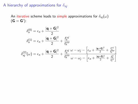
A hierarchy of approximations for δnj

An iterative scheme leads to simple approximations for δnj(ω)(G = G′):

δ(0)n = εn +|q + G|2

2

δ(1)n = εn +|q + G|2

2+

f ρjn

f ρρn

δ(2)nj (ω) = εn +

|q + G|2

2+

f ρjn

f ρρn

ω − ωj −[εn + |q+G|2

2 +f ρjn

f ρρn

]ω − ωj −

[εn + |q+G|2

2 + f jjnf ρjn

]

-The f ρρn , f ρjn , f jjn , · · · are simple with sums over occupied states only.

f ρjn =

[〈n|i∇|n〉 −

occ∑v

〈n|e i(q+G)·r|v〉〈v |e−i(q+G)·r′ [i∇]|n〉]· (q+ G)

-From δ(1)n onwards exact for the homogeneous electron gas.

-δ(2)nj (ω) simple but nontrivial due to frequency dependence.

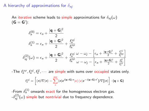
A hierarchy of approximations for δnj

An iterative scheme leads to simple approximations for δnj(ω)(G = G′):

δ(0)n = εn +|q + G|2

2

δ(1)n = εn +|q + G|2

2+

f ρjn

f ρρn

δ(2)nj (ω) = εn +

|q + G|2

2+

f ρjn

f ρρn

ω − ωj −[εn + |q+G|2

2 +f ρjn

f ρρn

]ω − ωj −

[εn + |q+G|2

2 + f jjnf ρjn

]-The f ρρn , f ρjn , f jjn , · · · are simple with sums over occupied states only.

f ρjn =

[〈n|i∇|n〉 −

occ∑v

〈n|e i(q+G)·r|v〉〈v |e−i(q+G)·r′ [i∇]|n〉]· (q+ G)

-From δ(1)n onwards exact for the homogeneous electron gas.

-δ(2)nj (ω) simple but nontrivial due to frequency dependence.

Getting δStarting from the definition:

S ≡empty∑

c

〈n|e i(q+G)·r|c〉〈c|e−i(q+G)·r′ |n〉ω − ωj − εc

=

empty∑c

〈n|e i(q+G)·r|c〉〈c|e−i(q+G)·r′ |n〉ω − ωj − δ

Rearranging:

δ = εn +

empty∑c

〈n|e i(q+G)·r|c〉〈c|e−i(q+G)·r′ |n〉(εc − εn)

ω − ωj − εc/S

The εi are eigenvalues of H with eigenstates |i〉:

δ = εn +∑c

〈n|e i(q+G)·r|c〉〈c|[H(r′), e−i(q+G)·r′ ]|n〉[ω − ωj − εc ]

/S

Working out the commutator:

[H(r), e−i(q+G)·r] = e−i(q+G)·r[|q + G|2

2+ (q + G) · i∇

]we obtain

δ = εn +|q + G|2

2+∑c

〈n|e i(q+G)·r|c〉〈c|e−i(q+G)·r′ [i∇]|n〉 · (q + G)

[ω − ωj − εc ]/S

Getting δStarting from the definition:

S ≡empty∑

c

〈n|e i(q+G)·r|c〉〈c|e−i(q+G)·r′ |n〉ω − ωj − εc

=

empty∑c

〈n|e i(q+G)·r|c〉〈c|e−i(q+G)·r′ |n〉ω − ωj − δ

Rearranging:

δ = εn +

empty∑c

〈n|e i(q+G)·r|c〉〈c|e−i(q+G)·r′ |n〉(εc − εn)

ω − ωj − εc/S

The εi are eigenvalues of H with eigenstates |i〉:

δ = εn +∑c

〈n|e i(q+G)·r|c〉〈c|[H(r′), e−i(q+G)·r′ ]|n〉[ω − ωj − εc ]

/S

Working out the commutator:

[H(r), e−i(q+G)·r] = e−i(q+G)·r[|q + G|2

2+ (q + G) · i∇

]we obtain

δ = εn +|q + G|2

2+∑c

〈n|e i(q+G)·r|c〉〈c|e−i(q+G)·r′ [i∇]|n〉 · (q + G)

[ω − ωj − εc ]/S

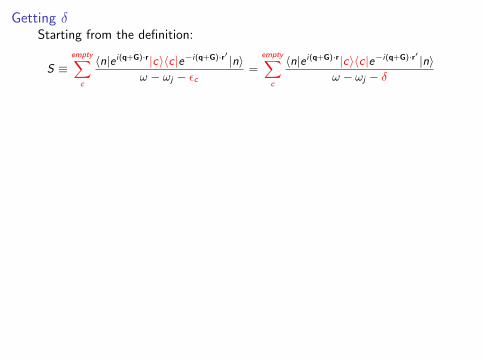
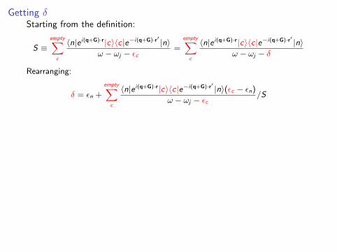
Getting δStarting from the definition:

S ≡empty∑

c

〈n|e i(q+G)·r|c〉〈c|e−i(q+G)·r′ |n〉ω − ωj − εc

=

empty∑c

〈n|e i(q+G)·r|c〉〈c|e−i(q+G)·r′ |n〉ω − ωj − δ

Rearranging:

δ = εn +

empty∑c

〈n|e i(q+G)·r|c〉〈c|e−i(q+G)·r′ |n〉(εc − εn)

ω − ωj − εc/S

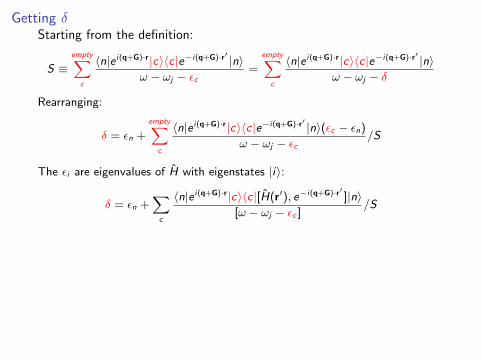
The εi are eigenvalues of H with eigenstates |i〉:

δ = εn +∑c

〈n|e i(q+G)·r|c〉〈c|[H(r′), e−i(q+G)·r′ ]|n〉[ω − ωj − εc ]

/S

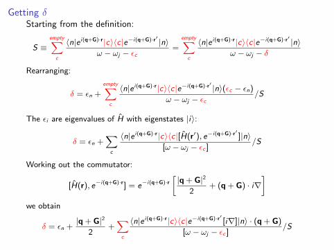
Working out the commutator:

[H(r), e−i(q+G)·r] = e−i(q+G)·r[|q + G|2

2+ (q + G) · i∇

]we obtain

δ = εn +|q + G|2

2+∑c

〈n|e i(q+G)·r|c〉〈c|e−i(q+G)·r′ [i∇]|n〉 · (q + G)

[ω − ωj − εc ]/S

Getting δStarting from the definition:

S ≡empty∑

c

〈n|e i(q+G)·r|c〉〈c|e−i(q+G)·r′ |n〉ω − ωj − εc

=

empty∑c

〈n|e i(q+G)·r|c〉〈c|e−i(q+G)·r′ |n〉ω − ωj − δ

Rearranging:

δ = εn +

empty∑c

〈n|e i(q+G)·r|c〉〈c|e−i(q+G)·r′ |n〉(εc − εn)

ω − ωj − εc/S

The εi are eigenvalues of H with eigenstates |i〉:

δ = εn +∑c

〈n|e i(q+G)·r|c〉〈c|[H(r′), e−i(q+G)·r′ ]|n〉[ω − ωj − εc ]

/S

Working out the commutator:

[H(r), e−i(q+G)·r] = e−i(q+G)·r[|q + G|2

2+ (q + G) · i∇

]we obtain

δ = εn +|q + G|2

2+∑c

〈n|e i(q+G)·r|c〉〈c|e−i(q+G)·r′ [i∇]|n〉 · (q + G)

[ω − ωj − εc ]/S

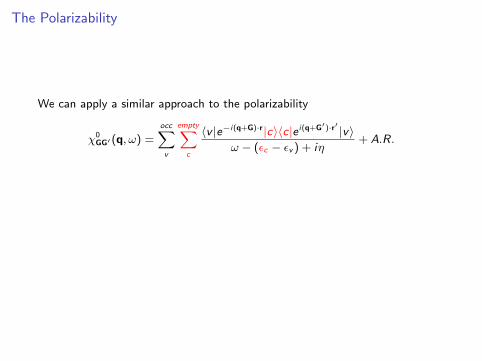
The Polarizability

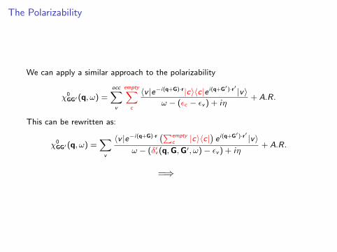
We can apply a similar approach to the polarizability

χ0GG′(q, ω) =

occ∑v

empty∑c

〈v |e−i(q+G)·r|c〉〈c|e i(q+G′)·r′ |v〉ω − (εc − εv ) + iη

+ A.R.

This can be rewritten as:

χ0GG′(q, ω) =

∑v

〈v |e−i(q+G)·r (∑emptyc |c〉〈c|

)e i(q+G′)·r′ |v〉

ω − (δ′v (q,G,G′, ω)− εv ) + iη+ A.R.

=⇒

The Polarizability

We can apply a similar approach to the polarizability

χ0GG′(q, ω) =

occ∑v

empty∑c

〈v |e−i(q+G)·r|c〉〈c|e i(q+G′)·r′ |v〉ω − (εc − εv ) + iη

+ A.R.

This can be rewritten as:

χ0GG′(q, ω) =

∑v

〈v |e−i(q+G)·r (∑emptyc |c〉〈c|

)e i(q+G′)·r′ |v〉

ω − (δ′v (q,G,G′, ω)− εv ) + iη+ A.R.

=⇒

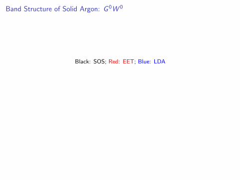
Band Structure of Solid Argon: G 0W 0

Black: SOS; Red: EET; Blue: LDA

SnO2: Band gap

LDA G 0W 0 G 0W 0 Experiment(SOS) (EET)

SnO2 (Eg ) 0.91 2.88 2.94 3.6

SOS: 1600 bands (Σ) EET: 34 valence bands

- Good agreement between SOS approach and EET.- G 0W 0 band gaps not in agreement with experiment.

Include self-consistency:GW = self-consistent COHSEX + G 0W 0 (Bruneval et al. PRB (2006))

LDA GW (EET) ExperimentSnO2 (Eg ) 0.91 3.8 3.6

SnO2: Band gap

LDA G 0W 0 G 0W 0 Experiment(SOS) (EET)

SnO2 (Eg ) 0.91 2.88 2.94 3.6

SOS: 1600 bands (Σ) EET: 34 valence bands

- Good agreement between SOS approach and EET.- G 0W 0 band gaps not in agreement with experiment.

Include self-consistency:GW = self-consistent COHSEX + G 0W 0 (Bruneval et al. PRB (2006))

LDA GW (EET) ExperimentSnO2 (Eg ) 0.91 3.8 3.6

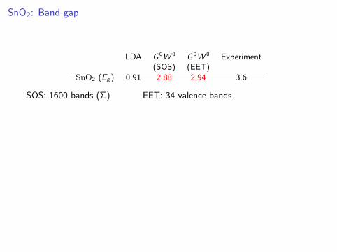
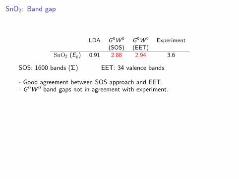
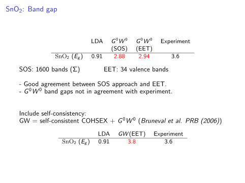
SnO2: Band gap

LDA G 0W 0 G 0W 0 Experiment(SOS) (EET)

SnO2 (Eg ) 0.91 2.88 2.94 3.6

SOS: 1600 bands (Σ) EET: 34 valence bands

- Good agreement between SOS approach and EET.- G 0W 0 band gaps not in agreement with experiment.

Include self-consistency:GW = self-consistent COHSEX + G 0W 0 (Bruneval et al. PRB (2006))

LDA GW (EET) ExperimentSnO2 (Eg ) 0.91 3.8 3.6

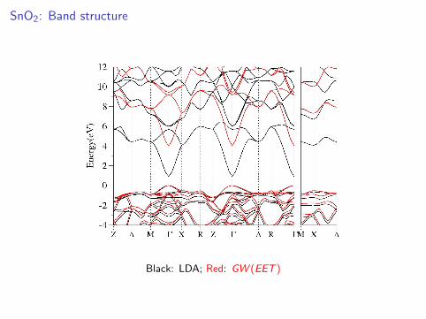
SnO2: Band structure

Black: LDA; Red: GW (EET )

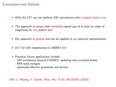
Conclusions and Outlook

I With the EET we can perform GW calculations with occupied states only.

I The approach is simple with immediate speed ups of at least an order ofmagnitude for any system size.

I Our approach is general and can be applied to any spectral representation.

I EET for GW implemented in ABINIT 6.4

I Potential future applications include:- Self-consistency beyond COHSEX: updating only occupied states.- RPA total energies- optimized effective potentials and kernels.

JAB, L. Reining, F. Sottile, Phys. Rev. B 82, 041103(R) (2010)

SnO2: Absorption tail