252 OPTICS LETTERS / Vol. 10, No. 6 / June 1985

Optical linear algebra processors:noise and error-source modeling

David Casasent and Anjan Ghosh*

Department of Electrical and Computer Engineering, Carnegie-Mellon University, Pittsburgh, Pennsylvania 15213

Received September 4, 1984; accepted March 21, 1985

The modeling of system and component noise and error sources in optical linear algebra processors (OLAP's) areconsidered, with attention to the frequency-multiplexed OLAP. General expressions are obtained for the outputproduced as a function of various component errors and noise. A digital simulator for this model is discussed.

Optical linear algebra processors (OLAP's) representa most attractive class of general-purpose optical pro-cessors with parallel and real-time features.1 The fre-quency-multiplexed OLAP2 is easily fabricated, permitsa competitive high computation rate, and with differentdata-encoding schemes allows all the basic operationsof linear algebra functions to be performed with excel-lent pipelining and flow of data.3 We thus emphasizethis architecture in our present study. Many OLAP'sthat operate on digital data have also been suggested.'These systems achieve the accuracy of a digital pro-cessor together with the speed and parallel-processingadvantages of optical systems. Despite this widespreadinterest, little attention4 has been given to an analysisand modeling of the various noise and error sources insuch optical architectures. We briefly review the fre-quency-multiplexed OLAP and the basic linear algebraoperations required. Then we detail the types of errorspossible in such a processor and derive our model fornoise- and error-source effects in OLAP's and the ex-pression for the output obtained as a function of thevarious system-component noise and errors. We dis-cuss digital simulation of this model and its use. Themodeling, simulation procedure, and general approachthat we use are valid for most OLAP's, including digi-tal-optical linear algebra processors.

A simplified diagram of the frequency-multiplexedOLAP is shown in Fig. 1. This architecture consists ofN input point modulators imaged through N separateregions of an acousto-optic (AO) cell (with each regionseparated by a bit time TB). The AO cell is fed with N1-D input signals, each on a different temporal-fre-quency carrier. We view these signals as N vectors,each on a spatial carrier. The light intensity distribu-tion leaving the cell is then the products of the inputvector (from the point modulators) and the N vectorsin the cell, with each such product leaving the cell at anangle proportional to the input frequency to the cell.The Fourier-transform (FT) lens sums the elements ofeach vector product (by space integration) and formseach of the N-vector inner products on a separate out-put detector. The detector output voltages (or cur-rents) are thus proportional to the (N X N) matrix-vector product, with one matrix-vector multiplicationperformed each TB.

If intensity-mode operation is used, the signals to be

processed are present on a bias. The effects of thesebias terms in the output data must be removed andcorrected for. The necessary correction signals can beeasily obtained with a separate adjunct processorchannel similar to the way in which bias was correctedin the initial optical matrix-vector processors usingtwo-dimensional masks. Amplitude-mode operationof the AO cells and the system is also possible and insome cases preferable. In the conventional system, thedetected output intensity will be the square of an am-plitude product, and thus the square root of the input(or output) data must be produced. Methods to achievethis exist, but coherent detection at the output is pref-erable. In this case, the detector output voltage isproportional to the desired amplitude product. Eithermode of operation requires attention to the choice offrequencies and their separation to ensure linearity andsuppression of cross talk. The effects of intermodula-tion-induced cross talk require further examination.

No delays exist in this processor since data flowcontinuously, as detailed elsewhere,3 even though thesame matrix remains in the AO cell for NTB. Withdifferent space (x), time (t), and frequency (f) encoding,matrix data can be processed by the system, and variousmatrix-vector, matrix-matrix, and matrix-matrix-matrix multiplications and iterative and direct solutionsof systems of linear algebra equations can be realized.3The basic operation performed by the system is thus amatrix-vector product each TB. This is the basicbuilding block of all other matrix operations and directand indirect solutions of linear and nonlinear algebraicequations.3 In this Letter, we describe our noise- anderror-source modeling of the frequency-multiplexedOLAP in terms of this basic Ab = c system opera-tion.

Fig. 1. Simplified schematic of a frequency-multiplexedoptical linear algebra processor. (After Ref. 2.)

0146-9592/85/060252-03$2.00/0 © 1985, Optical Society of America

June 1985 / Vol. 10, No. 6 / OPTICS LETTERS 253

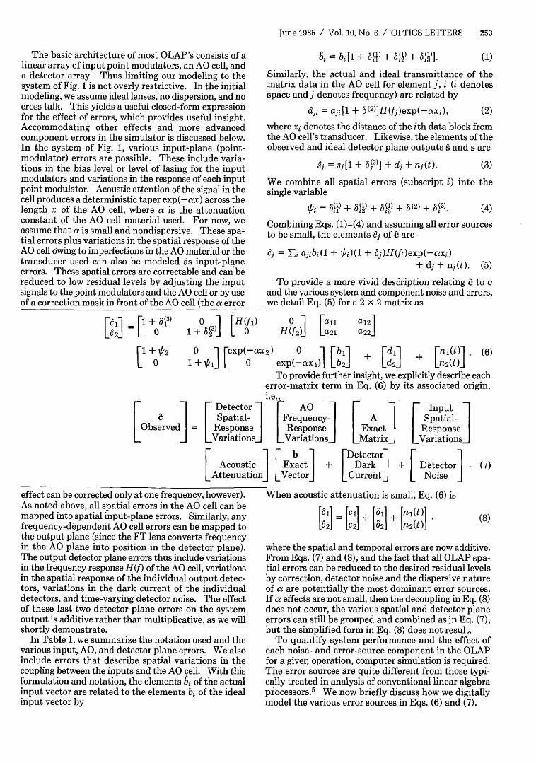
The basic architecture of most OLAP's consists of alinear array of input point modulators, an AO cell, anda detector array. Thus limiting our modeling to thesystem of Fig. 1 is not overly restrictive. In the initialmodeling, we assume ideal lenses, no dispersion, and nocross talk. This yields a useful closed-form expressionfor the effect of errors, which provides useful insight.Accommodating other effects and more advancedcomponent errors in the simulator is discussed below.In the system of Fig. 1, various input-plane (point-modulator) errors are possible. These include varia-tions in the bias level or level of lasing for the inputmodulators and variations in the response of each inputpoint modulator. Acoustic attention of the signal in thecell produces a deterministic taper exp(-ax) across thelength x of the AO cell, where a is the attenuationconstant of the AO cell material used. For now, weassume that a is small and nondispersive. These spa-tial errors plus variations in the spatial response of theAO cell owing to imperfections in the AO material or thetransducer used can also be modeled as input-planeerrors. These spatial errors are correctable and can bereduced to low residual levels by adjusting the inputsignals to the point modulators and the AO cell or by useof a correction mask in front of the AO cell (the a error

=i = bi [ + 6(l) + 852) + 6I3]. (1)

Similarly, the actual and ideal transmittance of thematrix data in the AO cell for element i, i (i denotesspace and j denotes frequency) are related by

aii = aji[l + 6(2 )]H(fj)exp(-avxi), (2)

where xi denotes the distance of the ith data block fromthe AO cell's transducer. Likewise, the elements of theobserved and ideal detector plane outputs A and s are

Sj = sj[l + b53)] + dj + nj(t). (3)

We combine all spatial errors (subscript i) into thesingle variable

Vi = a51 + (2) + a3) + 3(2) + 5 2)* (4)

Combining Eqs. (1)-(4) and assuming all error sourcesto be small, the elements 6j of c are

6j = Yi ajibi(l + #i)(l + 5j)H(fi)exp(-axi)+ dj + nj(t). (5)

To provide a more vivid description relating 6 to cand the various system and component noise and errors,we detail Eq. (5) for a 2 X 2 matrix as

[ti = [1+&p)

[ 1 t # 2O [ FH(fi)1 + 6N3) L °

0 1 [aH(f 2) La2n

a1 2 1a22J

[exp(-ax2) 0 1[bil + d1i + Fn1(t). (6)1 ++1 L ° exp(-axl)J Lb2 J Ln2(0 _

To provide further insight we explicitly describe eacherror-matrix term in .Eq. (6) by its associated origin,i.e.,ir _ Detector AO _Input

j Spatial- Frequency- A Spatial-Observed = Response Response Exact Response

_ariations _ Variations Matrix_[ b Detector F

Acoustic Exact + Dark + Detector (7)FAttenuation] [Vector] Current [ Noise

effect can be corrected only at one frequency, however).As noted above, all spatial errors in the AO cell can bemapped into spatial input-plane errors. Similarly, anyfrequency-dependent AO cell errors can be mapped tothe output plane (since the FT lens converts frequencyin the AO plane into position in the detector plane).The output detector plane errors thus include variationsin the frequency response H(f) of the AO cell, variationsin the spatial response of the individual output detec-tors, variations in the dark current of the individualdetectors, and time-varying detector noise. The effectof these last two detector plane errors on the systemoutput is additive rather than multiplicative, as we willshortly demonstrate.

In Table 1, we summarize the notation used and thevarious input, AO, and detector plane errors. We alsoinclude errors that describe spatial variations in thecoupling between the inputs and the AO cell. With thisformulation and notation, the elements bi of the actualinput vector are related to the elements bi of the idealinput vector by

When acoustic attenuation is small; Eq. (6) is

Oii = + 1611 + 1(0(8)

where the spatial and temporal errors are now additive.From Eqs. (7) and (8), and the fact that all OLAP spa-tial errors can be reduced to the desired residual levelsby correction, detector noise and the dispersive natureof a are potentially the most dominant error sources.If a effects are not small, then the decoupling in Eq. (8)does not occur, the various spatial and detector planeerrors can still be grouped and combined as in Eq. (7),but the simplified form in Eq. (8) does not result.

To quantify system performance and the effect ofeach noise- and error-source component in the OLAPfor a given operation, computer simulation is required.The error sources are quite different from those typi-cally treated in analysis of conventional linear algebraprocessors. 5 We now briefly discuss how we digitallymodel the various error sources in Eqs. (6) and (7).

254 OPTICS LETTERS / Vol. 10, No. 6 / June 1985

Table 1. SAOP Error Source Model

Error Source Notation

Spatial errors Subscript iFrequency errors Subscript jInput plane errors Superscript 1AO cell errors Superscript 2

Detector-plane errors Superscript 3

Input Plane Errors Notation

Point modulatorSpatial gain 1 + MVBias nonuniformity 1 + MV2)

Coupling (spatial) 1 + 613)

AO Cell Plane Errors Notation

Amplifier errors 1 + 6(2)

Spatial response 1 + 3f2)AO transfer function H(f1 )Acoustic attenuation exp(-axj)

Detector Plane Errors Notation

Spatial response 1 + a35)Dark current d,Time-varying noise nj(t)

From experiments on our laboratory OLAP systems,we found that the residual spatial errors and the de-tector noise can be modeled as zero-mean Gaussianrandom numbers and that signal-dependent (quantum)noise is not present. The frequency response H(f) andthe acoustic attenuation can be modeled as determin-istic errors that are quantified by measurements on theOLAP. This deterministic function multiplies thematrix data in the cell as in Eq. (6). Since the spatialerrors are independent of time, the random numbersrepresenting each such error are generated once bystandard IMSL6 or other software and stored. The 36standard deviation of each random number is chosento equal the percentage error to be modeled. For inputand AO cell spatial errors, the random numbers are in-cluded in each input vector datum b each TB, and fordetector spatial errors the associated random numbersare added to the computed output vector each TB as inEq. (6). For fixed or spatial errors, the same set ofrandom numbers is used at each TB. To simulate de-tector noise, a new set of uncorrelated variables withGaussian probability distribution is generated eachTB .

The model above and the form of the result in Eqs.(6)-(8) are useful for conveying error effects in closedform, for showing how various error sources can begrouped, and for noting which error sources are cor-rectable, multiplicative, and additive. Other errorsources and other models for the various componentscan be included directly in the simulator [but do notlend themselves to convenient diagonal matrices as inEq. (6) and to a closed-form expression for the system].Variations in the bias level of the point modulators andall errors are assumed to be small residual errors (aftercorrection). Thus bias-level variations are included inAi-. If such individual errors are not small, performance

will be too poor to consider. A primary purpose of ourinitial model and its simulator is to quantify the domi-nant error sources and the magnitude allowed for each(i.e., the level to which fixed spatial errors must becorrected and the amount of noncorrectable errors al-lowed).

For quantitative performance data, other advancedmodels can be used. Exact transfer curves (after cor-rection) for each point modulator and detector can bemeasured and used in the actual simulator. We havedone this and found the results (for the small residualerrors present in practice) to be the same as those ob-tained using our random variable modeling. To includethe dispersive nature of a, a different exp(-ax) factoris used for each signal in the AO cell. This is a fixedfactor (different for each frequency signal) that mul-tiplies the present spatial contents of the cell each TB.Our simulator includes this feature, but it is not con-veniently included in the equation formulations above.Similar remarks apply to cross-talk effects in the AO celland to the electronic circuit models.

From detailed simulations and analyses with themodel in Eq. (6), we found that acoustic attenuation anddetector noise are the dominant error sources. In initialsimulations,4 we found that a effects are dominant initerative algorithms and detector noise is dominant indirect algorithms. We also found that the effects ofsmall multiple-error sources are additive as in Eq.(8).

The various error sources that arise in an OLAP havebeen tabulated and grouped into two classes (correct-able or fixed and time-varying) and classified accordingto the plane (input, AO cell, output detectors) in whichthey originate. Combining these separate error sources,we find that error matrices in systolic processors aremultiplicative and that acoustic attenuation is an im-portant error source in OLAP's employing AO cells.The model and simulation technique advanced can andshould be applied to other OLAP's to quantify thedominant error sources, the effect of multiple errors,and the performance to be expected from each systemfor each application and algorithm.

The support of this research by NASA Lewis Re-search Center (grant NAG-3-5), the U.S. Air Force Of-fice of Scientific Research (grant 79-0091), and inde-pendent contractors of Unicorn Systems Incorporatedis gratefully acknowledged.

* Present address, AT&T Bell Laboratories, Allen-town, Pennsylvania 18103.

References

1. Special issue on optical computing, Proc. IEEE 72 (July1984).

2. D. Casasent, J. Jackson, and C. P. Neuman, Appl. Opt. 22,115 (1983).

3. D. Casasent, Proc. IEEE 72, 831 (1984).4. D. Casasent, A. Ghosh, and C. P. Neuman, Proc. Soc.

Photo-Opt. Instrum. Eng. 431, 201 (1983).5. J. Wilkinson, Rounding Errors in Algebraic Processes

(Wiley, New York, 1963).6. International Mathematics and Statistics Library Ref-

erence Manual, 8th ed. (IMSL, Houston, Tex., 1980).