Optic Flow and Motion Detection

Cmput 498/613Cmput 498/613

Martin JagersandMartin Jagersand

Readings: Papers and Readings: Papers and chapters on 613 web page chapters on 613 web page

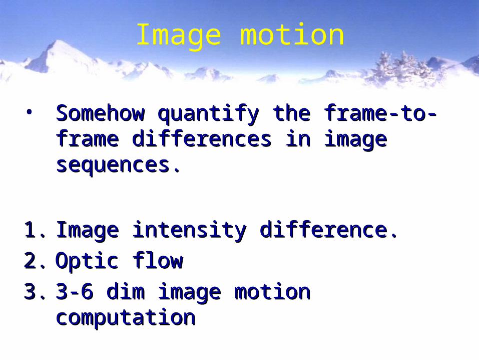
Image motion

• Somehow quantify the frame-to-frame Somehow quantify the frame-to-frame differences in image sequences.differences in image sequences.

1.1. Image intensity difference.Image intensity difference.

2.2. Optic flowOptic flow

3.3. 3-6 dim image motion computation3-6 dim image motion computation

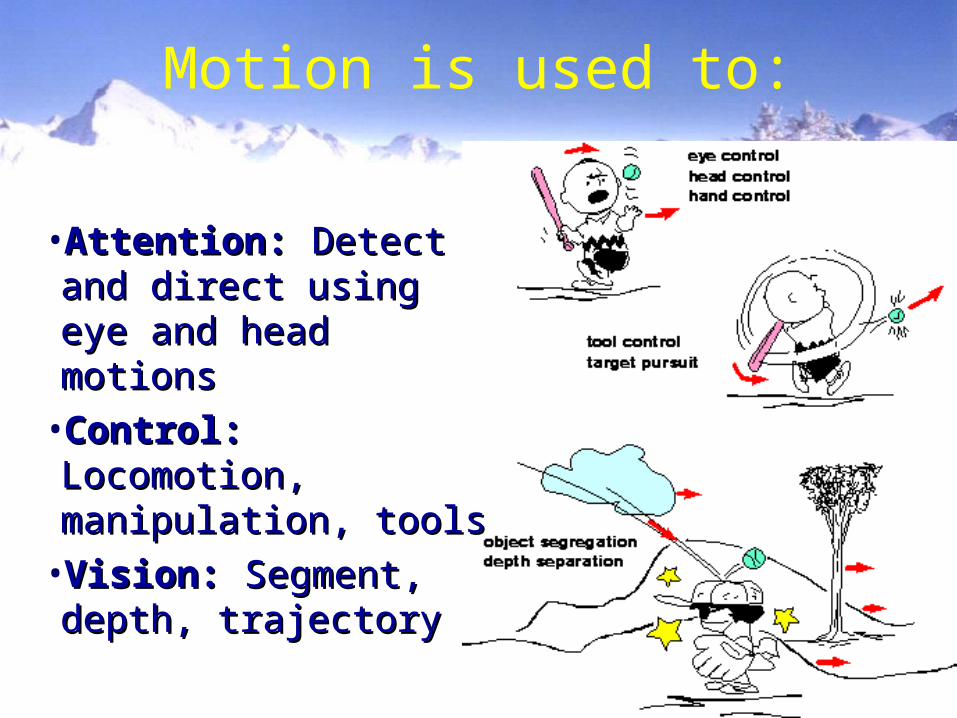
Motion is used to:

•Attention:Attention: Detect and Detect and direct using eye and direct using eye and head motions head motions

•Control:Control: Locomotion, Locomotion, manipulation, toolsmanipulation, tools

•Vision:Vision: Segment, depth, Segment, depth, trajectorytrajectory

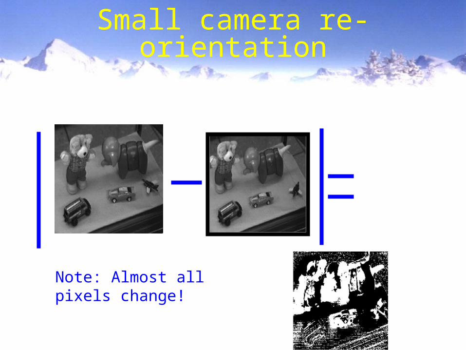
Small camera re-orientation

Note: Almost all pixels change!

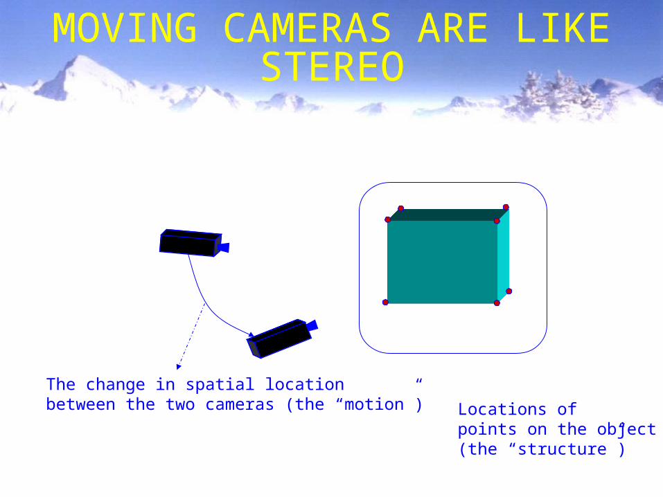
MOVING CAMERAS ARE LIKE STEREO

Locations ofpoints on the object(the “structure”)

The change in spatial locationbetween the two cameras (the “motion”)

Classes of motion

•Still camera, single moving objectStill camera, single moving object

•Still camera, several moving objectsStill camera, several moving objects

•Moving camera, still backgroundMoving camera, still background

•Moving camera, moving objectsMoving camera, moving objects

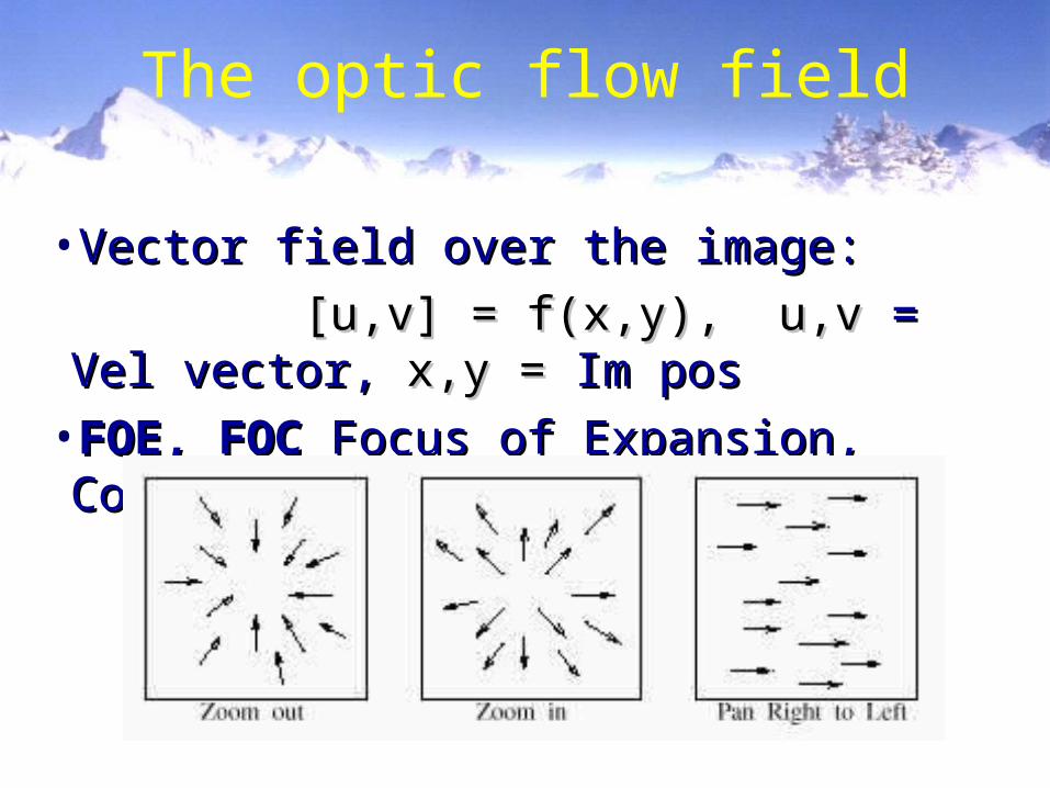
The optic flow field

•Vector field over the image:Vector field over the image:

[u,v] = f(x,y), u,v[u,v] = f(x,y), u,v = Vel vector, = Vel vector, x,y = x,y = Im posIm pos

•FOE, FOCFOE, FOC Focus of Expansion, Contraction Focus of Expansion, Contraction

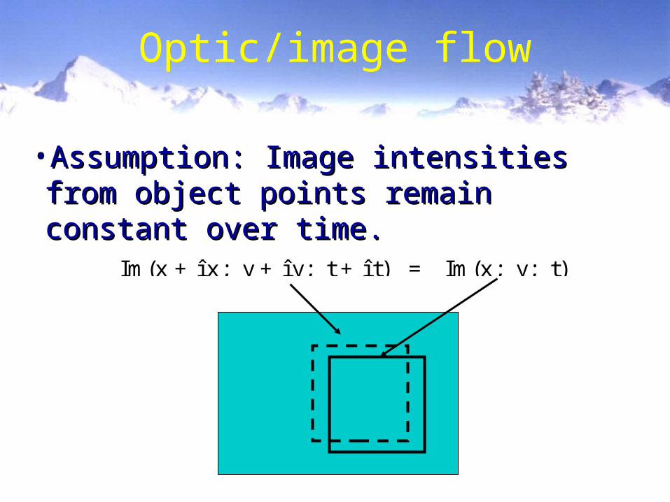
Optic/image flow

•Assumption: Image intensities from object points Assumption: Image intensities from object points remain constant over time.remain constant over time.

Im(x + î x; y + î y; t + î t) = Im(x; y; t)

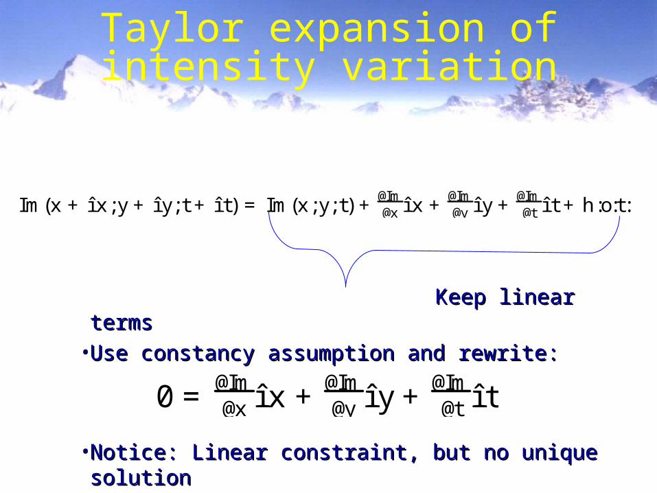
Taylor expansion of intensity variation

Keep linear termsKeep linear terms• Use constancy assumption and rewrite:Use constancy assumption and rewrite:

• Notice: Linear constraint, but no unique solutionNotice: Linear constraint, but no unique solution

à@t

@Im = @x@Im; @y

@Imð ñ

á î xî y

ò ó

0 = @x@Imî x + @y

@Imî y + @t@Imî t

Im(x + î x;y + î y; t + î t) = Im(x;y; t) + @x@Imî x + @y

@Imî y + @t@Imî t + h:o:t:

Im(x + î x;y + î y; t + î t) = Im(x;y; t) + @x@Imî x + @y

@Imî y + @t@Imî t + h:o:t:

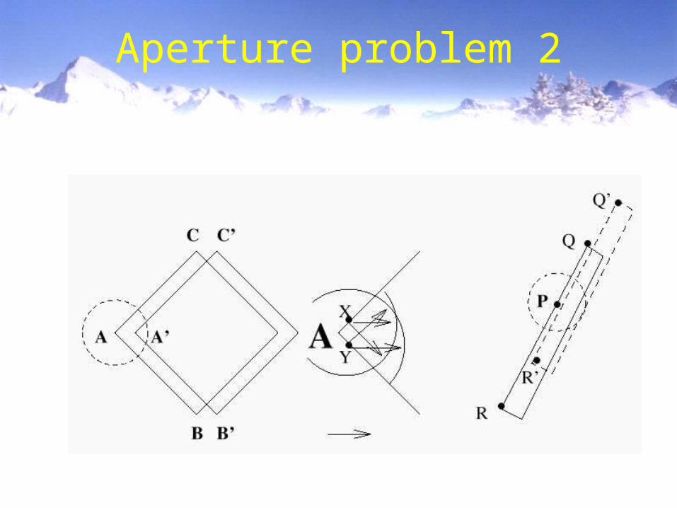
Aperture problem

• Rewrite as dot productRewrite as dot product

• Each pixel gives one equation in two unknowns:Each pixel gives one equation in two unknowns:f f . . n n = k= k

• Notice: Can only detect vectors normal to gradient Notice: Can only detect vectors normal to gradient directiondirection

• The motion of a line cannot be recovered using only The motion of a line cannot be recovered using only local informationlocal information

à @t@Im

= @x@Im ;@y

@Imð ñ á îxîy

ò ó= r Imá îx

îy

ò ó

fn

f

ît

Aperture problem 2

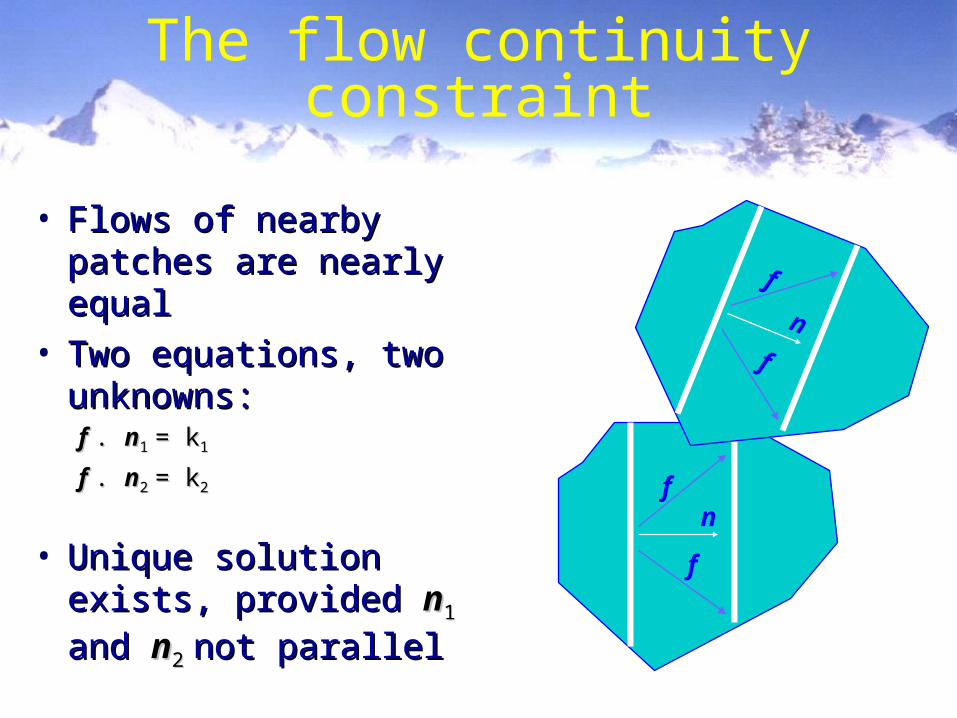
The flow continuity constraint

• Flows of nearby patches are Flows of nearby patches are nearly equalnearly equal

• Two equations, two Two equations, two unknowns:unknowns:f f . . nn11 = k= k11

f f . . nn22 = k= k22

• Unique solution exists, Unique solution exists, provided provided nn11 and and nn22 not not

parallelparallel

fn

f

f

n

f

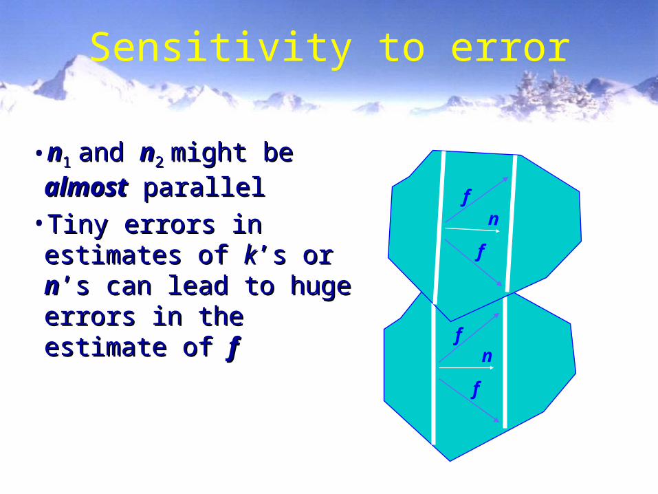
Sensitivity to error

• nn11 and and nn22 might be might be almostalmost

parallelparallel• Tiny errors in estimates of Tiny errors in estimates of kk’s ’s

or or nn’s can lead to huge errors ’s can lead to huge errors in the estimate of in the estimate of ff

fn

f

fn

f

Sometimes the continuity constraint is false

Using several points

•Typically solve for motion in 2x2, 4x4 or larger Typically solve for motion in 2x2, 4x4 or larger patches. patches.

•Over determined equation system:Over determined equation system:

dI = MudI = Mu•Can be solved in e.g. least squares sense using Can be solved in e.g. least squares sense using matlab matlab u = M\dIu = M\dI

...à

@t@Im

...

0

@

1

A =

......

@x@Im

@y@Im

......

0

@

1

A î xî y

ò ó

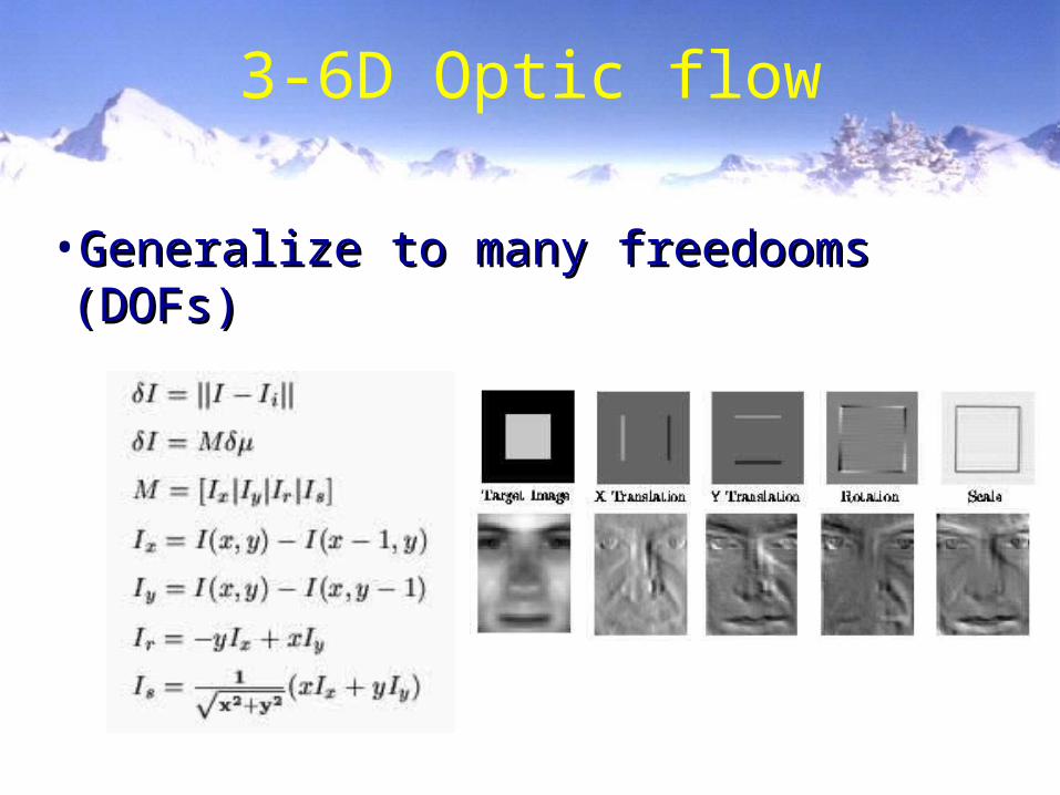
3-6D Optic flow

•Generalize to many freedooms (DOFs)Generalize to many freedooms (DOFs)

All 6 freedoms

X Y Rotation Scale Aspect Shear

M(u) = @Im=@u

M(u) = @Im=@u

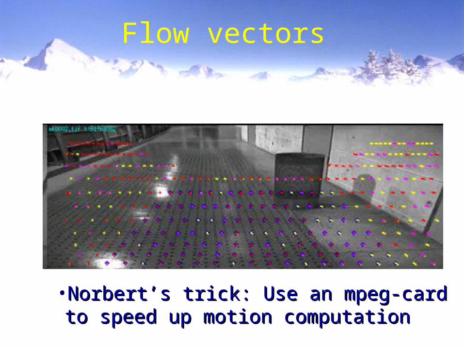
Flow vectors

•Norbert’s trick: Use an mpeg-card to speed Norbert’s trick: Use an mpeg-card to speed up motion computationup motion computation

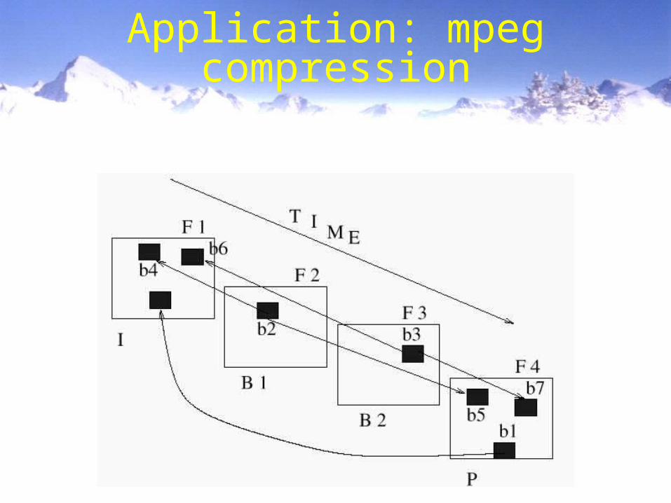
Application: mpeg compression

Other applications:

•Recursive depth recovery: Kostas Danilidis and Recursive depth recovery: Kostas Danilidis and Jane MulliganJane Mulligan

•Motion control (we will cover)Motion control (we will cover)

•SegmentationSegmentation

•TrackingTracking

Lab:

• Purpose:Purpose:– Hands on optic flow experienceHands on optic flow experience– Simple translation trackingSimple translation tracking

• Posted on www page.Posted on www page.• Prepare through readings: Prepare through readings:

(on-line papers.(on-line papers.• Lab tutorial: How to capture.Lab tutorial: How to capture.• Questions: Email or course Questions: Email or course

newsgroupnewsgroup• Due 1 week.Due 1 week.

Organizing different kinds of motion

Two ideas:Two ideas:

1.1. Encode different motion structure in the M-Encode different motion structure in the M-matrix. Examples in 4,6,8 DOF image plane matrix. Examples in 4,6,8 DOF image plane tracking. 3D a bit harder.tracking. 3D a bit harder.

2.2. Attempt to find a low dimensional subspace for Attempt to find a low dimensional subspace for the set of motion vectors. Can use e.g. PCAthe set of motion vectors. Can use e.g. PCA

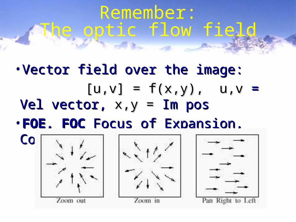
Remember:The optic flow field

•Vector field over the image:Vector field over the image:

[u,v] = f(x,y), u,v[u,v] = f(x,y), u,v = Vel vector, = Vel vector, x,y = x,y = Im posIm pos

•FOE, FOCFOE, FOC Focus of Expansion, Contraction Focus of Expansion, Contraction

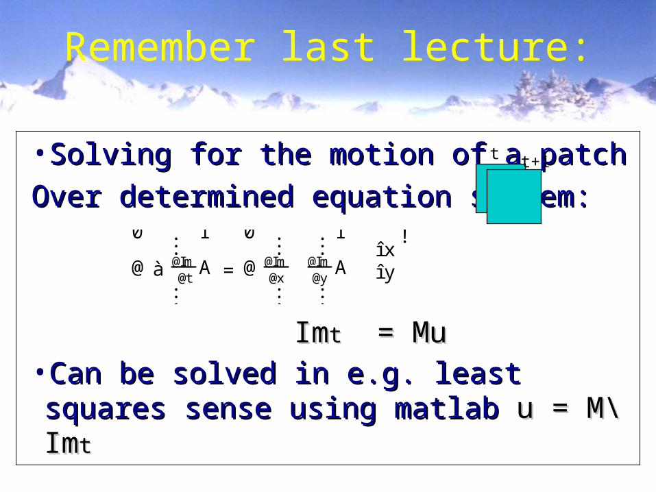
Remember last lecture:

•Solving for the motion of a patchSolving for the motion of a patch

Over determined equation system:Over determined equation system:

ImImtt = Mu = Mu•Can be solved in e.g. least squares sense using Can be solved in e.g. least squares sense using matlab matlab u = M\Imu = M\Imtt

...à

@t@Im

...

0

@

1

A =

......

@x@Im

@y@Im

......

0

@

1

Aî xî y

!

t t+1

3-6D Optic flow

•Generalize to many freedooms (DOFs)Generalize to many freedooms (DOFs)

Im = Mu

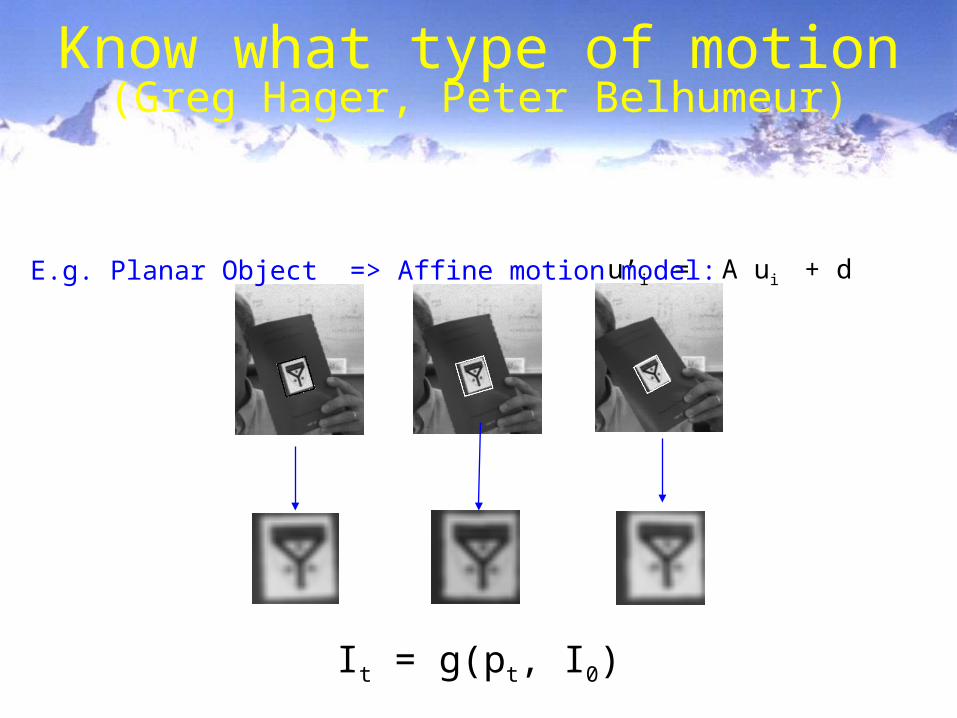
Know what type of motion(Greg Hager, Peter Belhumeur)

u’i = A ui + dE.g. Planar Object => Affine motion model:

It = g(pt, I0)

Mathematical Formulation

• Define a “warped image” Define a “warped image” gg– f(p,x) = x’f(p,x) = x’ (warping function), p warp parameters (warping function), p warp parameters– I(x,t)I(x,t) (image a location x at time t) (image a location x at time t)– g(p,Ig(p,Itt) = (I(f(p,x) = (I(f(p,x11),t), I(f(p,x),t), I(f(p,x22),t), … I(f(p,x),t), … I(f(p,xNN),t))’),t))’

• Define the Jacobian of warping functionDefine the Jacobian of warping function– M(p,t) =M(p,t) =

• ModelModel– II00 = g(p = g(ptt, I, It t )) (image I, variation model (image I, variation model gg, parameters , parameters pp))– I = I = MM(p(ptt, I, Itt) ) pp (local linearization (local linearization MM))

• Compute motion parametersCompute motion parameters p = (p = (MMT T MM))-1-1 MMT T I I where where MM = = MM(p(ptt,I,Itt))

@p@I

h i

Planar 3D motion

• From geometry we know that the correct From geometry we know that the correct plane-to-plane transform is plane-to-plane transform is

1.1. for a perspective camera the for a perspective camera the projective projective homographyhomography

2.2. for a linear camera (orthographic, weak-, para- for a linear camera (orthographic, weak-, para- perspective) the perspective) the affine warpaffine warp

uw

vw

" #

= Wa(p;a) =a3 a4

a5 a6

" #

p +a1

a2

" #

u0

v0

" #

= Wh(xh;h) = 1+h7u+h8v1

h1u h3v h5

h2u h4v h6

" #

Planar Texture Variability 1Affine Variability

•Affine warp functionAffine warp function

•Corresponding image variabilityCorresponding image variability

•Discretized for imagesDiscretized for images

= [B 1. . .B 6][y1; . . .;y6]T = Baya

É I a =P

i=16

@ai

@I wÉ ai = @u@I ;@v

@Iâ ã @a1

@u ááá @a6

@u

@a1

@v ááá @a6

@v

" # É a1...É a6

2

4

3

5

É I a = @u@I ;@v

@Iâ ã 1 0 ãu 0 ãv 00 1 0 ãu 0 ãv

" # y1...y6

2

4

3

5

uw

vw

" #

= Wa(p;a) =a3 a4

a5 a6

" #

p +a1

a2

" #

On The Structure of M

u’i = A ui + dPlanar Object + linear (infinite) camera

-> Affine motion model

X Y Rotation Scale Aspect Shear

M(p) = @g=@p

a3 a4

a5 a6

" #

= sR (Ê )a 00 1

" #1 0h 1

" #

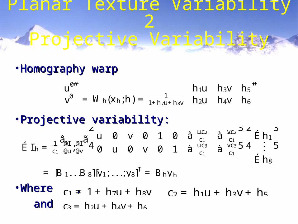
Planar Texture Variability 2Projective Variability

• Homography warpHomography warp

• Projective variability:Projective variability:

• WhereWhere ,,

and and

u0

v0

" #

= Wh(xh;h) = 1+h7u+h8v1

h1u h3v h5

h2u h4v h6

" #

É I h = c1

1@u@I ;@v

@Iâ ã u 0 v 0 1 0 à c1

uc2 à c1

vc2

0 u 0 v 0 1 à c1

uc3 à c1

vc3

2

4

3

5É h1...É h8

2

4

3

5

c1 = 1+ h7u + h8vc3 = h2u + h4v+ h6

c2 = h1u + h3v+ h5

= [B 1. . .B 8][y1; . . .;y8]T = Bhyh

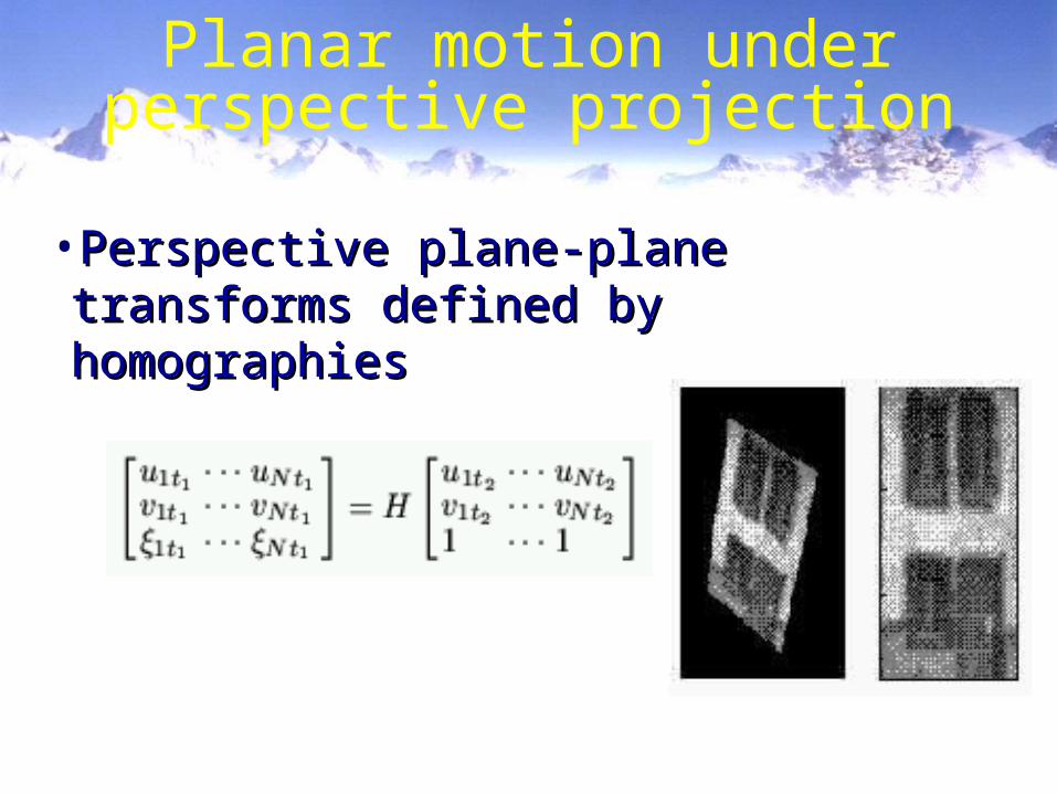
Planar motion under perspective projection

•Perspective plane-plane transforms defined by Perspective plane-plane transforms defined by homographieshomographies

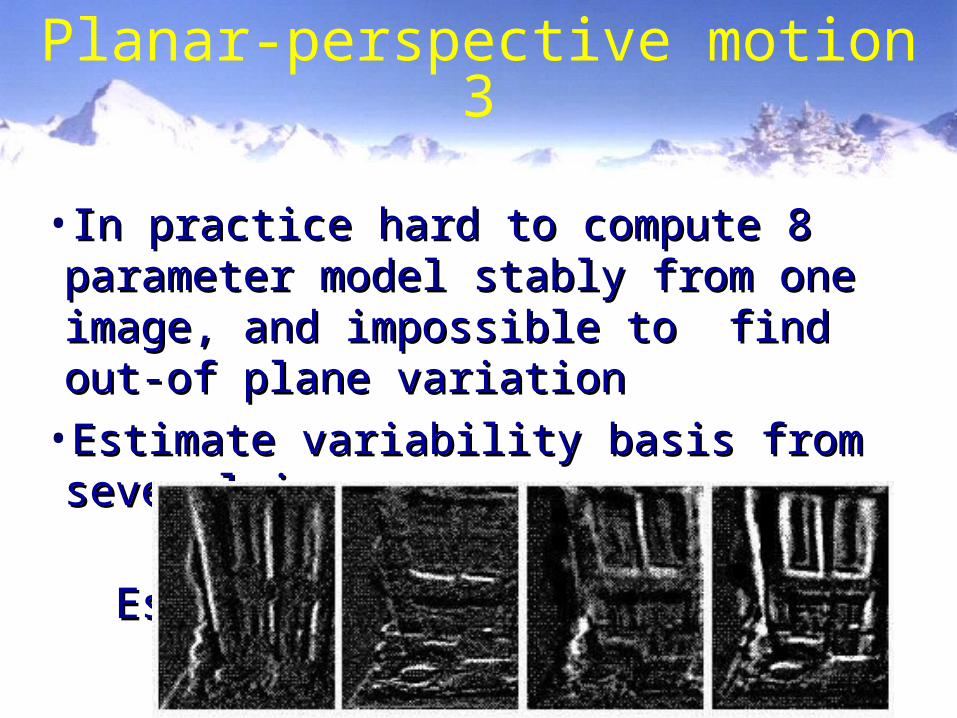
Planar-perspective motion 3

• In practice hard to compute 8 parameter model In practice hard to compute 8 parameter model stably from one image, and impossible to find stably from one image, and impossible to find out-of plane variationout-of plane variation

•Estimate variability basis from several images:Estimate variability basis from several images:

Computed EstimatedComputed Estimated

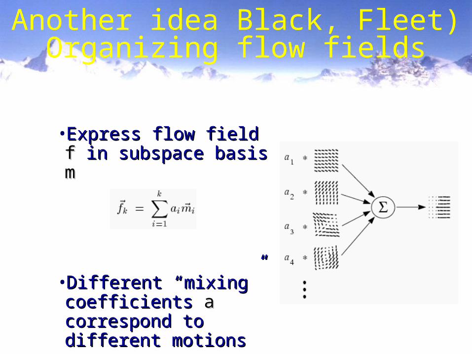
Another idea Black, Fleet) Organizing flow fields

•Express flow field Express flow field f f in in subspace basis subspace basis mm

•Different “mixing” Different “mixing” coefficients coefficients aa correspond to different correspond to different motionsmotions

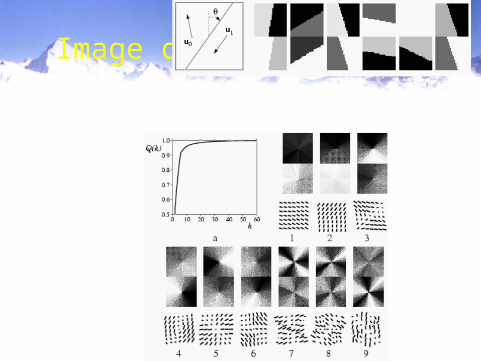
Example:Image discontinuities

Mathematical formulation

Let:Let:

Mimimize objective function:Mimimize objective function:

==

WhereWhere

Motion basis

Robust error norm

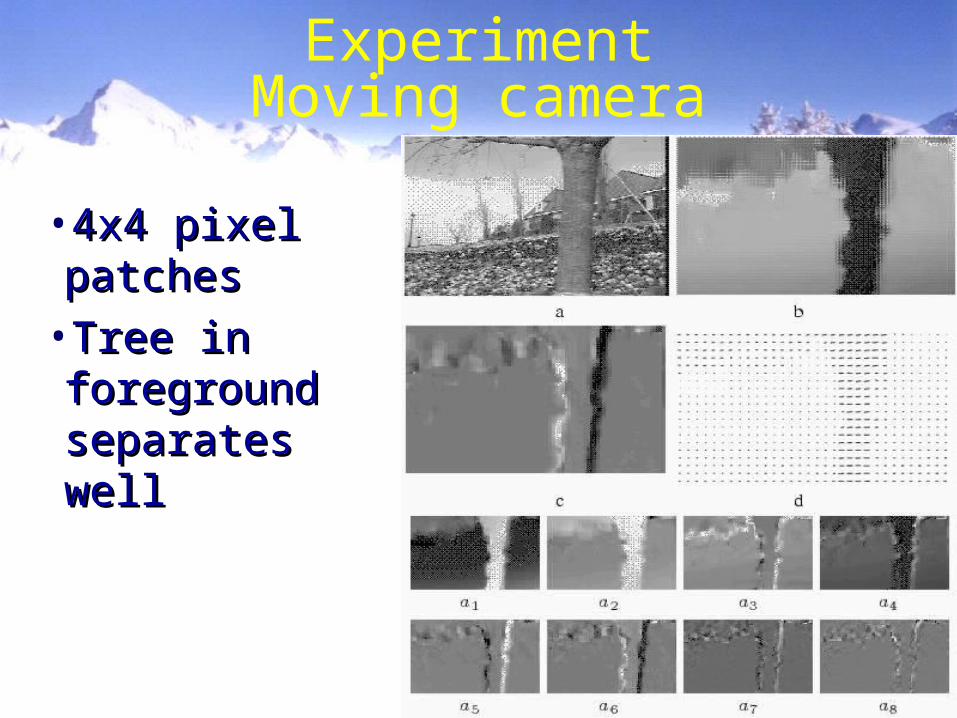
ExperimentMoving camera

•4x4 pixel 4x4 pixel patchespatches

•Tree in Tree in foreground foreground separates well separates well

Experiment:Characterizing lip motion

•Very non-rigid!Very non-rigid!

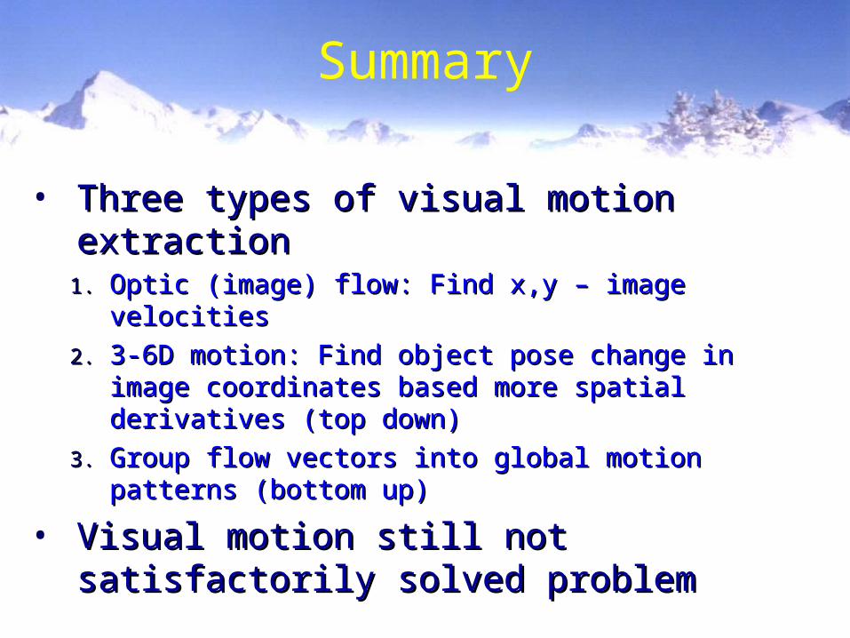
Summary

• Three types of visual motion extractionThree types of visual motion extraction1.1. Optic (image) flow: Find x,y – image velocitiesOptic (image) flow: Find x,y – image velocities

2.2. 3-6D motion: Find object pose change in image coordinates 3-6D motion: Find object pose change in image coordinates based more spatial derivatives (top down)based more spatial derivatives (top down)

3.3. Group flow vectors into global motion patterns (bottom up)Group flow vectors into global motion patterns (bottom up)

• Visual motion still not satisfactorily solved Visual motion still not satisfactorily solved problemproblem

Sensing and Perceiving Motionin Humans and Animals

Martin JagersandMartin Jagersand

How come perceived as motion?

Im = sin(t)U5+cos(t)U6 Im = f1(t)U1+…+f6(t)U6

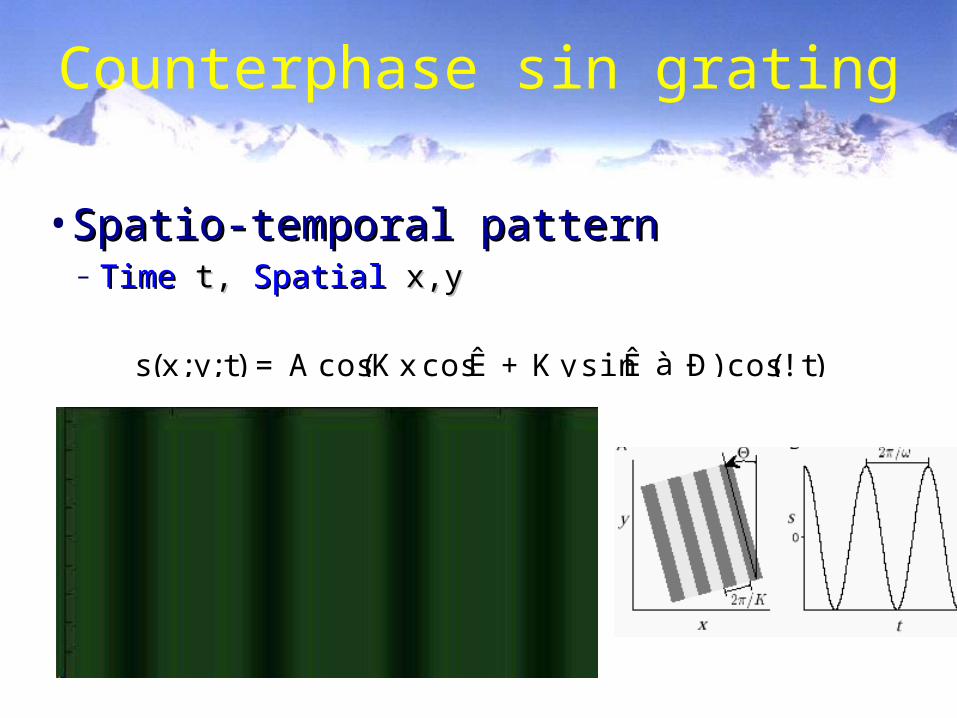
Counterphase sin grating

•Spatio-temporal patternSpatio-temporal pattern– Time Time t, t, Spatial Spatial x,yx,y

s(x;y;t) = A cos(K xcosÊ + K ysinÊ à Ð)cos(! t)

Counterphase sin grating

• Spatio-temporal patternSpatio-temporal pattern– Time Time t, t, Spatial Spatial x,yx,y

Rewrite as dot product:Rewrite as dot product:

= + = +

s(x;y;t) = A cos(K xcosÊ + K ysinÊ à Ð)cos(! t)

21(cos([a;b] x

y

ô õà ! t) + cos([a;b] x

y

ô õ+ ! t)

Result: Standing wave is superposition of two moving waves

Analysis:

•Only one term: Motion left or rightOnly one term: Motion left or right

•Mixture of both: Standing waveMixture of both: Standing wave

•Direction can flip between left and rightDirection can flip between left and right

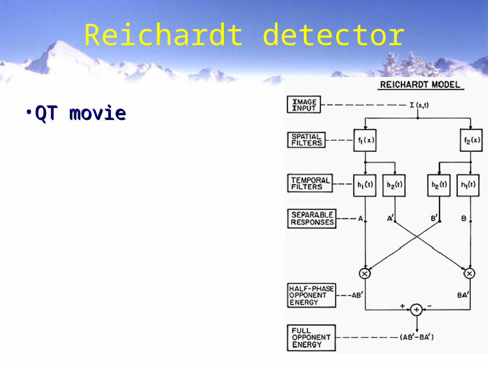
Reichardt detector

• QT movieQT movie

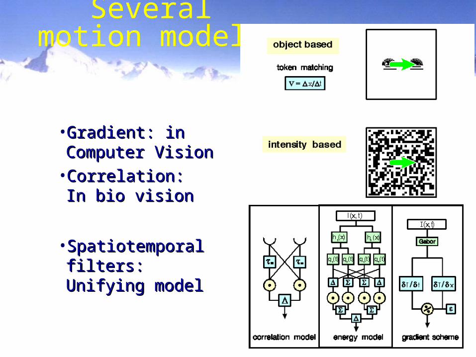
Severalmotion models

• Gradient: in Gradient: in Computer VisionComputer Vision

• Correlation: In bio Correlation: In bio visionvision

• Spatiotemporal Spatiotemporal filters: Unifying filters: Unifying modelmodel

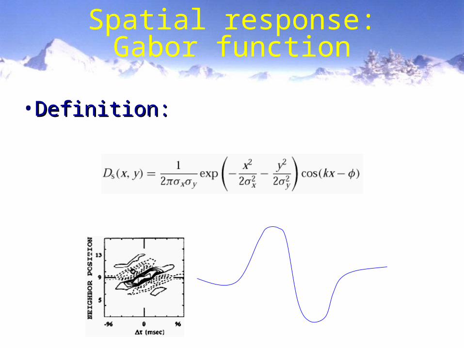
Spatial response:Gabor function

•Definition:Definition:

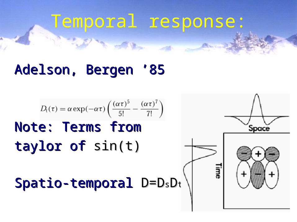
Temporal response:

Adelson, Bergen ’85Adelson, Bergen ’85

Note: Terms from Note: Terms from

taylor of taylor of sin(t)sin(t)

Spatio-temporal Spatio-temporal D=DD=DssDDtt

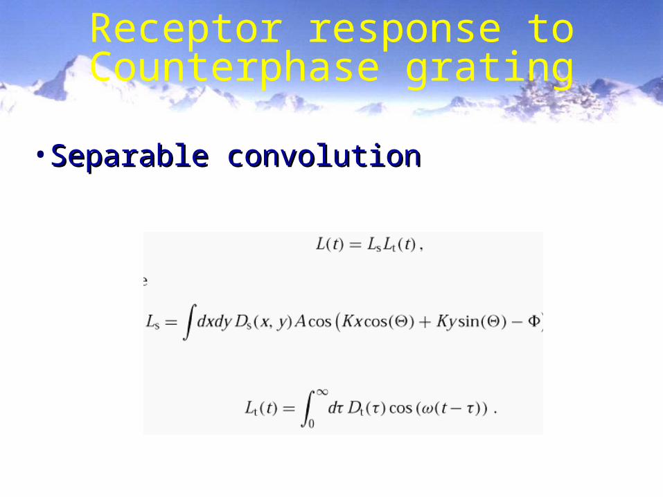
Receptor response toCounterphase grating

•Separable convolutionSeparable convolution

Simplified:

•For our grating: For our grating: (Theta=0)(Theta=0)

•Write as sum of components:Write as sum of components:

= exp(…)*(acos… + bsin…)= exp(…)*(acos… + bsin…)

L s = 2A exp 2

à û2(kà K )2ð ñ

cos(þ à Ð)

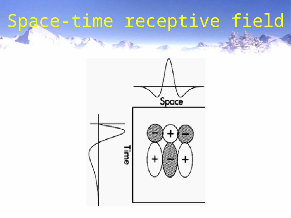
Space-time receptive field

Combined cells

• Spat: Temp:Spat: Temp:

• Both:Both:

• Comb:Comb:

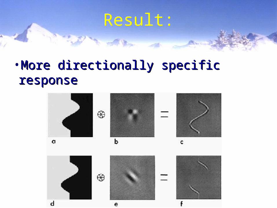
Result:

•More directionally specific responseMore directionally specific response

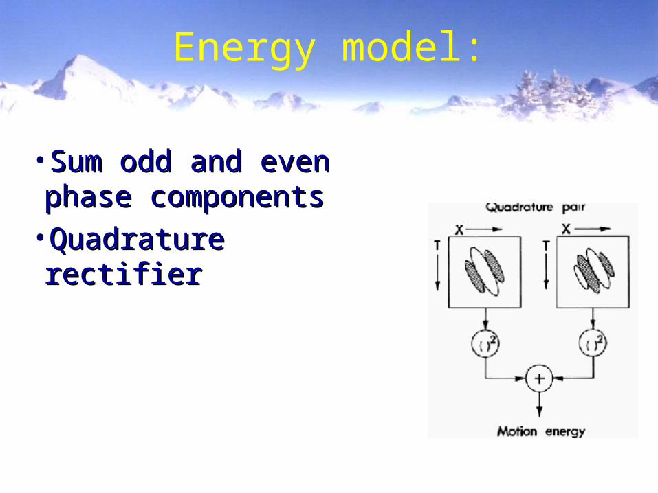
Energy model:

•Sum odd and even phase Sum odd and even phase componentscomponents

•Quadrature rectifierQuadrature rectifier

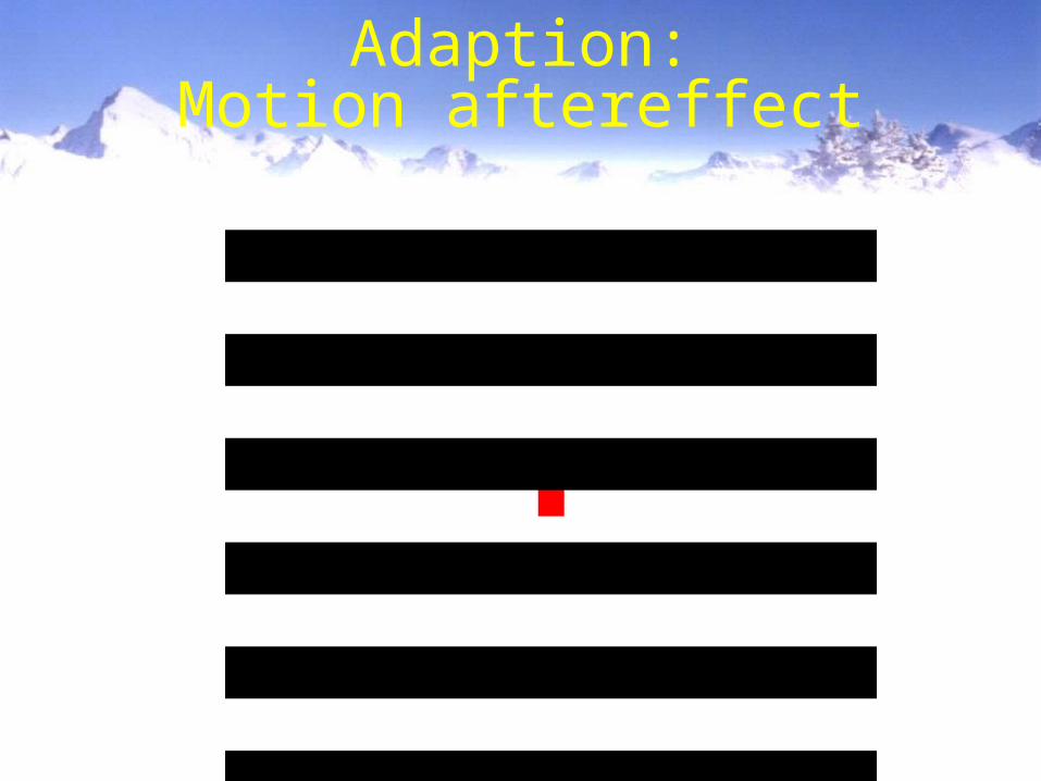
Adaption:Motion aftereffect

Where is motion processed?

Higher effects:

Equivalence:Reich and Spat

Conclusion

•Evolutionary motion detection is importantEvolutionary motion detection is important

•Early processing modeled by Reichardt detector Early processing modeled by Reichardt detector or spatio-temporal filters.or spatio-temporal filters.

•Higher processing poorly understoodHigher processing poorly understood