OPM, CAPM, and MM Theory

Presenter: 林崑峯 周立軒 劉亮志

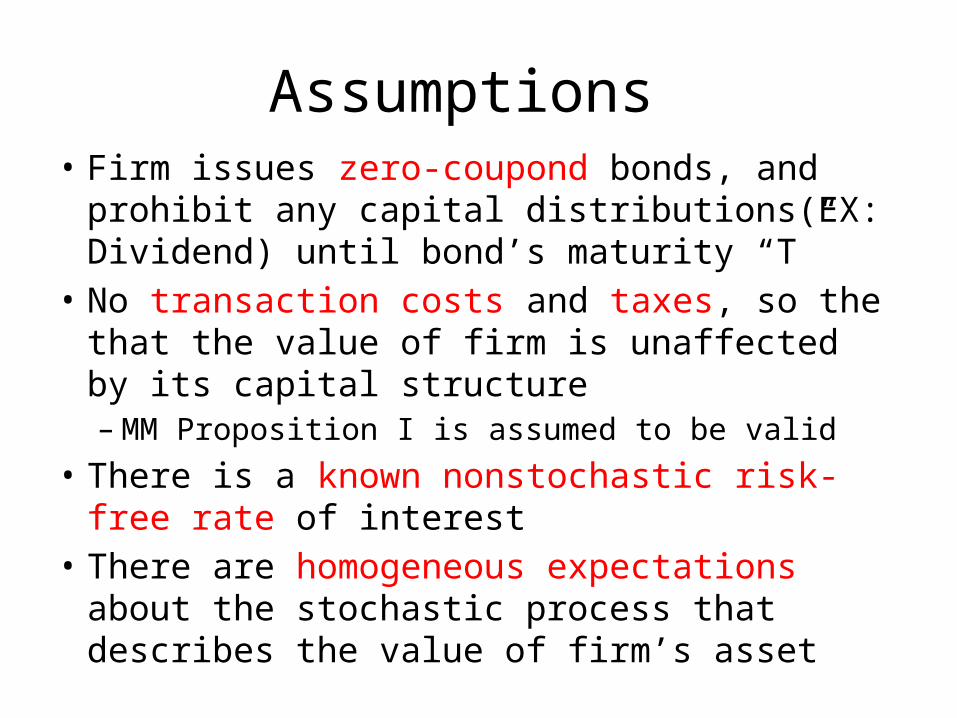
Assumptions • Firm issues zero-coupond bonds, and prohibit any

capital distributions(EX: Dividend) until bond’s maturity “T”

• No transaction costs and taxes, so the that the value of firm is unaffected by its capital structure– MM Proposition I is assumed to be valid

• There is a known nonstochastic risk-free rate of interest

• There are homogeneous expectations about the stochastic process that describes the value of firm’s asset

Merton’s Model• In Robert. C. Merton’s Asset Pricing Model,

the claims of Debt holders and Equity holders can be expressed by the following:

• For Debt Holders:

– Can be thought as the risk-free zero-copound bond (F), plus a Put in short position which underlying asset is firm’s asset (V) and its exercise price is (F)

– B = F - P

Merton’s Model• For Equity Holders:

– Can be viewed as a Call in long position which underlying asset is firm’s asset (V) and its exercise price is (F)

– S = C • Accounting Equation:– Asset = Debt + Equity – V = (F - P) + C– V + P = F + C

I-CAPM

• Because the OPM need continuous trading, but traditional CAPM is a one-period model. So we need I-CAPM as a connection between two models

B-S Call PDE

• Black and Scholes first derived the closed form solution for European Call’s value.

• If we divide Eq. 15.38 by S, and take limit on dt, we have:

Symbol change

• We recognize dS/S as the rate of return on common stock , . And dV/V as the rate of return on firm’s asset, . We have:

• And we know

sr

Vr

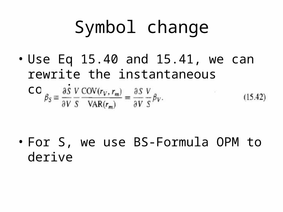
Symbol change

• Use Eq 15.40 and 15.41, we can rewrite the instantaneous covariance as

• For S, we use BS-Formula OPM to derive

BS Model (OPM)

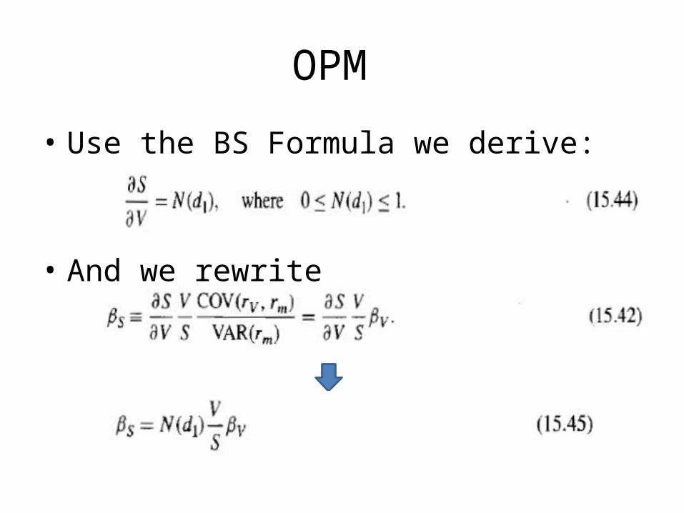
OPM

• Use the BS Formula we derive:

• And we rewrite

OPM

• For S, use OPM, we finally derive

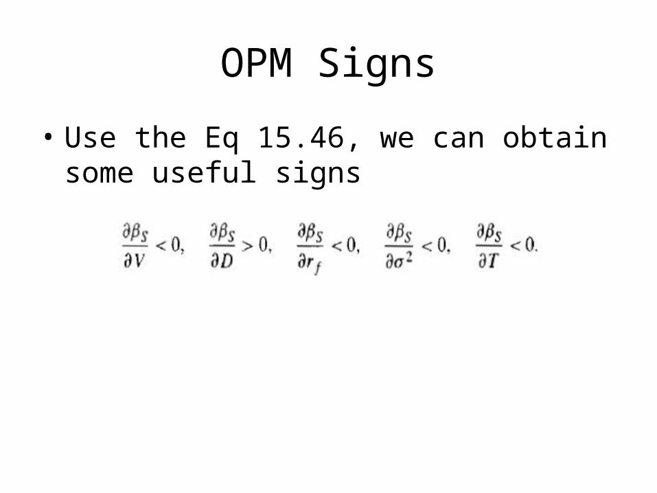
OPM Signs

• Use the Eq 15.46, we can obtain some useful signs

OPM vs CAPM

• Substituting from into the CAPM, we obtain

– Recall that – And since

– We obtain

S

OPM vs CAPM vs MM Propositions

• If we assume debts are risky and zero bankruptcy cost, the OPM, CAPM, and MM Propositions can be shown to be consistent.

• First, we start from , the systematic risk of risky debt in a world without taxes, can be expressed as

B

OPM vs CAPM vs MM Propositions• And recall Eq 15.44, the firm’s equity can be

thought as a call option on firm’s asset

– This two fact imply

• And we know the required rate of return of risky debt, can be expressed in CAPM form

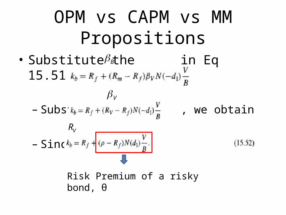
OPM vs CAPM vs MM Propositions

• Substitute the in Eq 15.51, we have

– Substitute the , we obtain

– Since = ρ (See P.575)

B

V

VR

Risk Premium of a risky bond, θ

OPM vs CAPM vs MM Propositions

6.3%, When D/V = 1

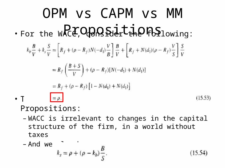
OPM vs CAPM vs MM Propositions• For the WACC, consider the following:

• This result is match the MM Propositions: – WACC is irrelevant to changes in the capital structure

of the firm, in a world without taxes– And we also have

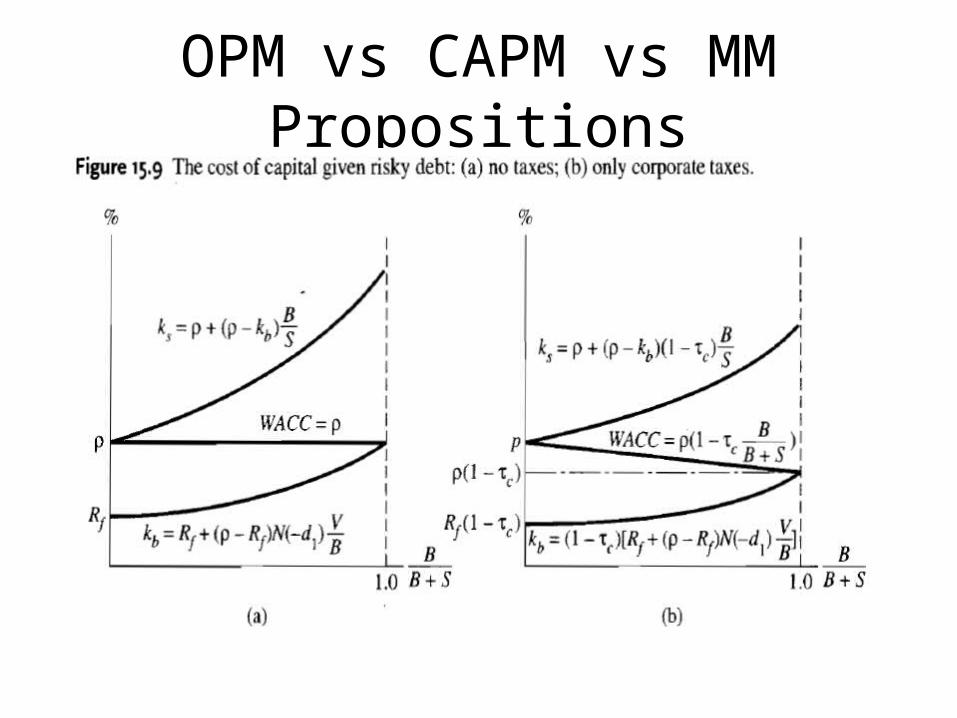
OPM vs CAPM vs MM Propositions

The Separability of Investment and Financial Decisions

• The fundamental assumption of MM is that operating cash flows are unaffected by the choice of capital structure – But this is challenged in the last decade– Debt increase may affect the credit

• The debt capability needs to be consider– Different debt capability of projects may cause

that we cannot treat investments and financial decisions as they are independent