DRSTP/LOTN School, Driebergen, April 2010

OPERATORS IN QUANTUM AND CLASSICAL OPTICS

Gerard NienhuisHuygens Laboratorium, Universiteit Leiden, Postbus 9504, 2300 RA Leiden∗

I. MAXWELL’S EQUATIONS FOR RADIATION AND COULOMB FIELD

A. Radiation and Coulomb modes of electromagnetic field

We consider a closed system of charged particles and the electromagnetic field. We wish to express the equationsof motion in a form that makes its quantization trivial. Maxwell’s equations can be represented in two homogeneousequations and two inhomogeneous ones. The homogeneous equations do not contain sources, and they take the form

~∇ · ~B = 0 ; ~∇× ~E +∂

∂t~B = 0 . (1.1)

The inhomogeneous equations in vacuum and in the presence of point charges are

~∇× ~B =1c2

( ∂

∂t~E +

~j

ε0

); ~∇ · ~E =

ρ

ε0. (1.2)

Sources of the fields are the charge density ρ and the current density ~j, defined by

ρ(~r) =∑α

qαδ(~r − ~rα) , ~j(~r) =∑α

qα~rαδ(~r − ~rα) . (1.3)

The homogeneous equations are automatically respected when one introduces a vector potential ~A and a scalarpotential Φ, so that

~B = ~∇× ~A , ~E = − ∂

∂t~A− ~∇Φ , (1.4)

The definition of mode functions is induced by the second inhomogeneous equation (1.2) in terms of the potentials

~∇× (~∇× ~A) =1c2

(− ∂2

∂t2~A− ∂

∂t~∇Φ +

1ε0

~j)

. (1.5)

Mode functions ~Mν are introduced by the eigenvector relation

~∇× (~∇× ~Mν) =ω2

ν

c2~Mν . (1.6)

We define the inner product of two vector functions ~F and ~G as the integral∫

d~r ~F ∗ · ~G. With this definition, theleft-hand side of (1.6) can be viewed as the square of a hermitian operator ~∇×. . ., which proves that its eigenvalues arenon-negative. This definition (1.6) of modes remains valid in the presence of reflecting boundaries, as in a cavity. Thenthe mode functions ~Mν must obey appropriate boundary conditions. In free space, the modes form a continuum. Forsimplicity, we denote the modes as a discrete set. This can be enforced by the standard procedure of selecting a largerectangular quantization volume V , and impose periodic boundary conditions. Alternatively, discrete summationscan be read as integration over a continuum of mode numbers.

∗Electronic address: nienhuis@molphys.leidenuniv.nl

2

We separate the space of mode functions in the subspace with eigenvalue zero, and the subspace with positiveeigenvalues. The subspace with eigenvalues zero spans the Coulomb space, with basis functions ~Cµ. The subspacewith non-zero eigenvalues is called the radiation space, with basis functions ~Rλ. These two subspaces are mutuallyorthogonal, since they correspond to non-overlapping sets of eigenvalues of a Hermitian operator. We express theeigenvalue relations as

~∇× (~∇× ~Cµ) = 0 , ~∇× (~∇× ~Rλ) =ω2

λ

c2~Rλ (ωλ > 0) . (1.7)

When we take the divergence ~∇ · . . . of the last equality in (1.7), we find that the radiation modes ~Rλ have vanishingdivergence, whereas the first equation (1.7) shows that the Coulomb modes ~Cµ have vanishing curl. Hence

~∇× ~Cµ = 0 , ~∇ · ~Rλ = 0 . (1.8)

Since the combination of Coulomb modes ~Cµ and radiation modes ~Rλ span the whole of function space, any vectorfield ~F is expanded in a unique way in the mode functions. Its projection on Coulomb space is called ~FC , and itsprojection on radiation space is ~FR, with

~FC =∑

µ

~CµFµ , ~FR =∑

λ

~RλFλ

with Fµ =∫

d~r ~C∗µ · ~F , Fλ =∫

d~r ~R∗λ · ~F . This separation of function space corresponds to a separation of the vectorfield ~F = ~FC + ~FR into a longitudinal (curl-free) part ~FC and a transverse (divergence-free) part ~FR. The presentformulation proves that this separation is unique and complete. A similar separation is valid in the presence ofmacroscopic non-dissipative media.

We use the freedom of gauge to make the vector potential divergence free, so that ~∇ · ~A = 0, and ~A = ~AR. Theequations (1.4) can now be reexpressed as

~B = ~BR = ~∇× ~A , ~ER = − ∂

∂t~A , ~EC = −~∇~Φ . (1.9)

This gives separate equations for the radiation and Coulomb parts of the electric field ~E, whereas the magnetic field~B has no Coulomb part.

B. Coulomb field

The inhomogeneous Maxwell equations (1.2) gives for the Coulomb part of ~E

∂

∂t~EC = − 1

ε0~jC , ~∇ · ~EC =

ρ

ε0.

This shows directly that the charge and current density ρ and ~jC are related by the continuity equation

∂

∂tρ = −~∇ ·~jC

(= −~∇ ·~j

).

Moreover, one notices that ~EC is just the Coulomb field corresponding to the instantaneous locations of the chargedparticles. Since the Coulomb field is curl-free, it lies indeed in Coulomb space. We conclude that the Coulomb contri-bution to ~E is fixed by the instantaneous positions of the charges, and it moves along with them. This demonstratesthat the Coulomb field ~EC is not an independent degree of freedom. It is simply determined by the charges. Thisinstantaneous relation between the charge positions and the Coulomb field indicates that the separation in radiationand Coulomb field is not relativistically invariant.

C. Radiation field and equations of motion

The radiation part of eq. (1.5) gives

~∇2 ~A =1c2

( ∂2

∂t2~A− 1

ε0~jR

), (1.10)

3

where we used that ~∇× (~∇× ~A) = −~∇2 ~A for the divergence-free vector potential. Apparently, the radiation part ofthe current ~jR is the source of ~A, which in turn determines the radiation field ~ER and ~B. The motion of the particlesis determined by the Coulomb force and the Lorentz force

mα~rα = qα

(~E(~rα) + ~rα × ~B(~rα)

). (1.11)

The independent degrees of freedom of the closed system of particles and fields are the particle positions ~rα and theradiation part of the vector potential ~AR(~r), specified by Aλ. The state of the system is fully described by ~rα,~rα, Aλ and Aλ. When the state is known at any instant of time, the equations of motion (1.10) and (1.11)completely determine the state in the future as well as in the past.

II. HAMILTONIAN DESCRIPTION AND QUANTIZATION

A. Radiation Hamiltonian and normal variables

As found above, the state of the radiation field at any instant of time is fully specified by the two variables Aλ andAλ. Alternatively, these can be represented as the single complex normal variable

aλ =√

ε02~ωλ

(ωλAλ + iAλ) .

Conversely, the set aλ determines both ~A and ~ER by

~A =∑

λ

√~

2ε0ωλ(aλ

~Rλ + a∗λ ~R∗λ) , ~ER = − ~A =∑

λ

√~ωλ

2ε0i(aλ

~Rλ − a∗λ ~R∗λ) . (2.1)

Note that the proof of (2.1) is not completely trivial. One may have to use that the vector potential ~A is real, andthat the eigenfunctions ~Rλ can be chosen real.

The total energy of the system of particles and fields separates in two contributions: one from the radiation fieldand one from the particles, including the Coulomb energy. After use of eq. (1.9) for ~B and ~ER, the radiation-fieldcontribution is written as

HR =12

∫d~r(ε0 ~E2

R +1µ0

~B2) =12

∑

λ

~ωλ(a∗λaλ + aλa∗λ) . (2.2)

The equations of motion for a mode of the free field are identical to those of a harmonic oscillator. The variables Aλ

and ε0Aλ serve as generalized canonical coordinate and momentum for the mode. The remaining energy is the kineticenergy of the particles (which is the sum of mα~r

2

α/2) and the Coulomb field energy (arising from ~EC). With somestraightforward algebra this can be expressed as

Hp =∑α

12mα

(~pα − qα

~A(~rα))2

+ VC . (2.3)

Here VC is the Coulomb interaction energy of the particles, which arises from the Coulomb field energy ε0∫

d~r ~E2C/2.

The quantity ~pα = mα~rα + qα~A(~rα) serves as the canonical momentum of particle α in the radiation field. It is

rewarding (and not trivial) to verify that the classical Hamilton equations xβ = ∂H/∂pβ , pβ = −∂H/∂xβ for thegeneralized coordinates and momenta of particles and fields with the total Hamiltonian H = HR+Hp indeed reproducethe equations of motion (1.10) and (1.11). This shows that the total energy actually serves as the Hamitonian interms of the generalized coordinates and momenta. Conservation of energy is then automatic.

B. Quantization

Now that we have reexpressed the equations of motion (Maxwell’s equations for the fields, and Newton’s law forthe particles) in a canonical Hamiltonian form, quantization has become trivial: just treat the generalized canonical

4

coordinates and momenta as operators, with the commutation rules [pβ , xβ′ ] = δββ′ . For the particles this impliesthat ~pα = (~/i)(∂/∂~rα). The normal field variables turn into field operators, for which the canonical commutationrules produce the well-known rules [aλ, a†λ′ ] = −i~δλλ′ .

Equations (2.1), (2.2) and (2.3) remain valid with the replacement a∗λ → a†λ. Specifically, the quantum operatorsfor the vector potential becomes

~A =∑

λ

√~

2ε0ωλ(aλ

~Rλ + a†λ ~R∗λ) , (2.4)

while the electric and the magnetic field take the form

~ER =∑

λ

√~ωλ

2ε0i(aλ

~Rλ − a†λ ~R∗λ) , ~B =∑

λ

√~

2ε0ωλ(aλ

~∇× ~Rλ + a†λ~∇× ~R∗λ) . (2.5)

The Hamiltonian of the radiation field is

HR ==12

∑

λ

~ωλ(a†λaλ + aλa†λ) . (2.6)

In the Schrodinger picture, the evolution of the quantum system is governed by the Schrodinger equation−(~/i)(d/dt)|Ψ〉 = H|Ψ〉 for the state vector |Ψ〉. In the Heisenberg picture, any physical quantity G obeys the equa-tion of motion (d/dt)G = (i/~)[H, G]. The Heisenberg equations of motion for the operators ~pα, ~rα and aλ closelyresemble the classical equations of motion for the corresponding classical variables, corresponding to Maxwell’s equa-tions for the fields, and Newton’s law with the Coulomb-Lorentz force for the particles. For instance, the evolution ofthe field operators is found as

d

dtaλ −−iωλaλ +

i

~

√~

2ε0ωλ

∑α

qαˆ~rα · ~R∗λ(~rα) , (2.7)

with ˆ~rα =

(~pα − qα

~A(~rα))/mα. This confirms that only the radiative part of the current is a source of the field. In

the absence of sources, the Heisenberg equation (2.7) is simply daλ/dt = −− iωλaλ.It is remarkable that the coupling between the fields and the particles in the Hamiltonian arises only in the kinetic-

energy terms in (2.3), which contain the products −qα~A · ~pα/mα. Note that the argument ~rα of ~A is also a quantum

operator.In free space, it is customary to choose the modes of the radiation field as plane-wave modes. Then the index λ

defines a mode of the radiation field, which takes the form of a normalized vector function

~Rλ(~r) =1√V

~eλei~kλ·~r . (2.8)

The mode is a plane wave, with wave vector ~k, and a normalized polarization vector ~eλ that is normal to ~kλ. Foreach wave vector, there are two independent polarization vectors. This reflects the transverse nature of the radiationfield. The wave vectors are discrete, and for a cubic quantization volume V = L3 with side L they take the values~kλ = 2π(nx, ny, nz)/L, with integer nx, ny and nz. The mode functions form a complete set of orthonormal transversevector functions on the volume V . With this expression for the modes, the field operators (2.4) and (2.5) attain theirstandard form.

III. SEPARATION OF ANGULAR MOMENTUM OF RADIATION FIELD

A. Classical description

From Maxwell’s theory it is well-known that the electromagnetic field has a density of momentum ε0 ~E × ~B. Theintegrated contribution from the Coulomb field ~EC combined with the kinetic momentum contributes to the totalcanonical momentum

∑α ~pα of the charged particles. The momentum density of the radiation field is ε0 ~ER × ~B.

5

From now on, we only consider the radiation field, and we shall suppress the index R on the electric field ~E and theangular momenta. The angular momentum of the radiation field, which is

~J = ε0

∫d~r ~r × ( ~E × ~B) =

∫d~r ~j . (3.1)

This expression can be separated after expressing the magnetic field in the vector potential and applying partialintegration [1]. This leads to the result

~J = ~L + ~S , (3.2)

with

~L = ε0∑

i

∫d~r Ei(~r × ~∇)Ai , ~S = ε0

∫d~r ~E × ~A . (3.3)

Since ~A is the transverse vector potential, these quantities are independent of gauge. The contribution ~L varies withthe choice of the origin, just as an orbital angular momentum, so that it has an extrinsic nature. Moreover, it isdetermined by the phase gradient of the field. On the other hand, the contribution ~S does not change for a differentchoice of the origin, and it is determined by the polarization of the field. This gives it the flavor of a spin angularmomentum.

B. Quantum operators

The expressions (3.3) for the contributions ~L and ~S to the angular momentum of the radiation field are quitesuggestive for their interpretation as orbital and spin parts. However, this interpretation is problematic. This is clearwhen we consider the quantized version of the system. It is convenient to choose circular polarization vectors ~e±(~k)in the plane normal to the wave vector ~k. The helicity of the vector ~e+ is parallel to ~k, whereas ~e− has opposite

helicity. The quantum operator for the quantity ~S is obtained by substituting the quantum operators ~A and ~E in theexpression (3.3). The result can be put in the intuitively attractive form [2, 3]

~S =∑

~k

~~k

k

(a†+(~k)a+(~k)− a†−(~k)a−(~k)

). (3.4)

This simply illustrates that each photon with wave vector ~k and polarization vector ~e+(~k) contributes to ~S a unit ~,in the direction of ~k. A photon with the opposite circular polarization ~e− gives the opposite contribution.

An obvious property of the quantum operator ~S is that its three components Sx, Sy and Sz commute, simplybecause the creation and annihilation operators for different modes commute. In fact, number states of all modes

with circular polarization are common eigenstates of all three components. This implies that ~S cannot be viewed as

a proper angular momentum operator, which generates rotations. On the other hand, the operator ~J is an angularmomentum momentum operator, as is exemplified by the commutation rule [Jx, Jy] = i~Jz, etc. As a result, the

commutation rules for the components of the quantum operator ~L take the form [2, 4]

[Lx, Ly] = i~(Lz − Sz) , (3.5)

etc. These remarkable commutation properties can be traced back to the fact that a rotation of the polarizationof a radiation field without rotating the field pattern itself would violate the transversality of the field. The vector

operator ~S is a proper quantum operator within the space of physical states. Its transformation properties resemblea rotation of the polarization pattern only insofar as it is allowed within the constraint of transversality [4].

IV. STATES OF FREE FIELD MODE

A. Number states

The states of a single mode of the radiation field are mathematically equivalent to the states of a free harmonicoscillator. A single mode is described by the Hamiltonian H = ~ω(a†a + 1

2 ), with the commutation rule [a, a†] = 1.

6

(The mode index λ is suppressed.) From the commutation rules it follows that the energy eigenstates are the numberstates |n〉, with n = 0, 1, . . ., so that a|n〉 =

√n|n − 1〉, a†|n〉 =

√n + 1|n + 1〉, a†a|n〉 = n|n〉. These states are

stationary, and therefore highly non-classical: they have a well-determined field amplitude, and a fully undetermined

phase. The expectation values of the fields ~E, ~A and ~B are zero. The ground state |0〉 is also called the vacuum state.But the fluctuations ∆ ~E, ∆ ~A and ∆ ~B are non-zero, even in the vacuum state. The number n indicates the numberof elementary excitations (photons) of the mode. Each photon represents an energy ~ω. Photons as elementaryexcitations of a single mode are just as delocalized as the mode function ~R. Localized single-photon states can beformed as superpositions of single-photon states in different modes, such as

∑cλ|λ〉, with |λ〉 the state |n〉 with n = 1

in the mode λ.

B. Coherent states

The states |z〉 that correspond most closely to classical states have (average) field values as given in (2.1) with areplaced by the complex number z. They are defined by the requirement

〈z|a|z〉 = z , 〈z|a†a|z〉 = |z|2 .

This implies the eigenvalue relation a|z〉 − z|z〉 = 0, with the solution

|z〉 = exp(−12|z|2)

∑n

zn

√n!|n〉 . (4.1)

According to Eq. (4.1), in a coherent state the probability distribution Pn over the number states is

Pn = e−|z|2 |z|2n

n!. (4.2)

This is a Poissonian distribution, with average value 〈n〉 = |z|2. The variance of a Poissonian distribution is equal toits average, so that

∆n2 ≡ 〈n2〉 − 〈n〉2 = 〈n〉 = |z|2 . (4.3)

The coherent states are normalized by definition. However, they are not orthogonal. Their overlap can be directlyevaluated from the expansion (4.1), with the result

〈z|z′〉 = exp(−1

2|z|2 − 1

2|z′|2 + z∗z′

), (4.4)

so that the strength of the overlap has a simple Gaussian shape |〈z|z′〉|2 = exp(−|z − z′|2). Moreover, the coherent

states are overcomplete: each state of the mode can be expanded in coherent states, but this expansion is not unique.One expansion can be found by applying the closure relation

I =1π

∫d2z |z〉〈z| , (4.5)

where the integration extends over the complex plane. The operator I is the unit operator for the mode.The uncertainty in a coherent state is best specified by the introducing quadrature operators

X =1√2(a + a†) , Y =

1i√

2(a− a†) ,

which obey the commutation relation [X, Y ] = i, and therefore the uncertainty relation ∆X∆Y ≥ 12 . In a coherent

state, ∆X = ∆Y = 1/√

2, for all values of z. Hence the uncertainty is equally divided over the two quadratures, and∆X and ∆Y have the same value as in the vacuum state.

Coherent states can alternatively be described as a displaced vacuum state

|z〉 = D(z)|0〉 , (4.6)

with

D(z) = exp(za† − z∗a) . (4.7)

The displacement properties of D(z) follow from the identity D†(z)aD(z) = a + z.

7

X

Y

X

Y

D

D

U

U

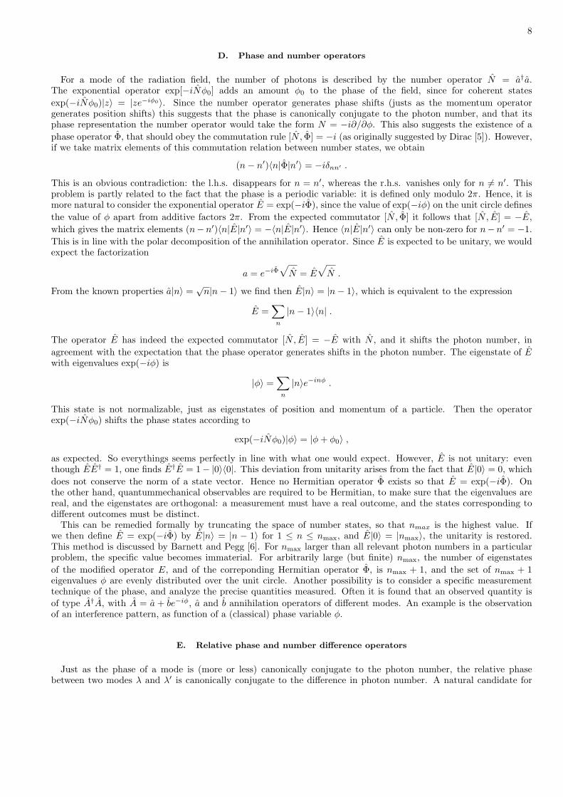
amplitude squeezing phase squeezing

FIG. 1: Illustration in the XY -plane of the shape of amplitude and phase squeezed states. These can be created by applyinga displacement to a squeezed vacuum state.

C. Squeezed states

We introduce the unitary squeeze operator

S(ξ) = exp(12ξ∗a2 − 1

2ξa†2) ,

for arbitrary complex number ξ = ρ exp(iθ). It transforms the field operator a as

S†(ξ)aS(ξ) = a cosh ρ− a† exp(iθ) sinh ρ .

The rotated quadrature operators

ˆX = X cosθ

2+ Y sin

θ

2, ˆY = −X sin

θ

2+ Y cos

θ

2then transform according to

S†(ξ) ˆXS(ξ) = ˆXe−ρ , S†(ξ) ˆY S(ξ) = ˆY eρ . (4.8)

Hence S effectively multiplies the quadrature components by scalar factors. The squeezed vacuum state S(ρ)|0〉 forξ = ρ real has a reduced uncertainty ∆X, and an enhanced uncertainty ∆Y , with ∆X∆Y = 1

2 unmodified.Squeezed coherent states arise when a displacement operator is applied to the squeezed vacuum state, and we

consider the free evolution of the initial state |ψ(0)〉 = D(z)S(ξ)|0〉. For positive ξ, the long axis of the ellipse isin the Y -direction, so that initially the ellipse is vertically oriented. When z is taken real, the center of the ellipselies on the X-axis at time zero. During free evolution, this ellipse rotates in the clockwise direction, at the angularvelocity ω. This is illustrated in Figure 1 on the left. In this case, the fluctuations in X are reduced at the times thatthe expectation value 〈X〉 is maximal. This means that the amplitude fluctuations are reduced compared with thevacuum fluctuations, which are the same as in a coherent state. This is called amplitude squeezing. The reduction ofthe amplitude fluctuations is compensated by an enhancement of phase fluctuations.

Conversely, when z is taken imaginary, the center of the ellipse lies initially on the Y -axis, and the uncertaintyin a quadrature is maximal when its expectation value passes a maximum. This is the case of enhanced amplitudefluctuations, and phase squeezing. This situation is pictured in the Figure 1 on the right.

These results show how a combination of squeezing S(ξ) (pumping that is quadratic in the ladder operators),displacement D(z) (pumping that is linear in the ladder operators), and free evolution U(t) acting on a vacuumstate creates minimum-uncertainty states. The uncertainty ellipses can have arbitrary ellipticity (determined by ξ),arbitrary locations in phase space (determined by z), and arbitrary orientation (determined by the angle ωt).

It is important to realize that the squeezed vacuum state is not a vacuum state, since it has a non-vanishingexpectation value of the photon number. By using (4.8) one finds that

〈0|S†(ρ)N S(ρ)|0〉 =12〈0|X2e−2ρ + Y 2e2ρ − 1|0〉 =

12

(cosh(2ρ)− 1) = sinh2 ρ . (4.9)

Reduction in the fluctuations in a quadrature below the vacuum fluctuations is possible, but not without the creationof photons in a special way.

8

D. Phase and number operators

For a mode of the radiation field, the number of photons is described by the number operator N = a†a.The exponential operator exp[−iNφ0] adds an amount φ0 to the phase of the field, since for coherent statesexp(−iNφ0)|z〉 = |ze−iφ0〉. Since the number operator generates phase shifts (justs as the momentum operatorgenerates position shifts) this suggests that the phase is canonically conjugate to the photon number, and that itsphase representation the number operator would take the form N = −i∂/∂φ. This also suggests the existence of aphase operator Φ, that should obey the commutation rule [N , Φ] = −i (as originally suggested by Dirac [5]). However,if we take matrix elements of this commutation relation between number states, we obtain

(n− n′)〈n|Φ|n′〉 = −iδnn′ .

This is an obvious contradiction: the l.h.s. disappears for n = n′, whereas the r.h.s. vanishes only for n 6= n′. Thisproblem is partly related to the fact that the phase is a periodic variable: it is defined only modulo 2π. Hence, it ismore natural to consider the exponential operator E = exp(−iΦ), since the value of exp(−iφ) on the unit circle definesthe value of φ apart from additive factors 2π. From the expected commutator [N , Φ] it follows that [N , E] = −E,which gives the matrix elements (n− n′)〈n|E|n′〉 = −〈n|E|n′〉. Hence 〈n|E|n′〉 can only be non-zero for n− n′ = −1.This is in line with the polar decomposition of the annihilation operator. Since E is expected to be unitary, we wouldexpect the factorization

a = e−iΦ√

N = E√

N .

From the known properties a|n〉 =√

n|n− 1〉 we find then E|n〉 = |n− 1〉, which is equivalent to the expression

E =∑

n

|n− 1〉〈n| .

The operator E has indeed the expected commutator [N , E] = −E with N , and it shifts the photon number, inagreement with the expectation that the phase operator generates shifts in the photon number. The eigenstate of Ewith eigenvalues exp(−iφ) is

|φ〉 =∑

n

|n〉e−inφ .

This state is not normalizable, just as eigenstates of position and momentum of a particle. Then the operatorexp(−iNφ0) shifts the phase states according to

exp(−iNφ0)|φ〉 = |φ + φ0〉 ,

as expected. So everythings seems perfectly in line with what one would expect. However, E is not unitary: eventhough EE† = 1, one finds E†E = 1− |0〉〈0|. This deviation from unitarity arises from the fact that E|0〉 = 0, whichdoes not conserve the norm of a state vector. Hence no Hermitian operator Φ exists so that E = exp(−iΦ). Onthe other hand, quantummechanical observables are required to be Hermitian, to make sure that the eigenvalues arereal, and the eigenstates are orthogonal: a measurement must have a real outcome, and the states corresponding todifferent outcomes must be distinct.

This can be remedied formally by truncating the space of number states, so that nmax is the highest value. Ifwe then define E = exp(−iΦ) by E|n〉 = |n − 1〉 for 1 ≤ n ≤ nmax, and E|0〉 = |nmax〉, the unitarity is restored.This method is discussed by Barnett and Pegg [6]. For nmax larger than all relevant photon numbers in a particularproblem, the specific value becomes immaterial. For arbitrarily large (but finite) nmax, the number of eigenstatesof the modified operator E, and of the correponding Hermitian operator Φ, is nmax + 1, and the set of nmax + 1eigenvalues φ are evenly distributed over the unit circle. Another possibility is to consider a specific measurementtechnique of the phase, and analyze the precise quantities measured. Often it is found that an observed quantity isof type A†A, with A = a + be−iφ, a and b annihilation operators of different modes. An example is the observationof an interference pattern, as function of a (classical) phase variable φ.

E. Relative phase and number difference operators

Just as the phase of a mode is (more or less) canonically conjugate to the photon number, the relative phasebetween two modes λ and λ′ is canonically conjugate to the difference in photon number. A natural candidate for

9

nλ

nλ ’

00

FIG. 2: Sketch of the 9 different number states of the two modes with N = 8 photons.

the exponential operator F = exp(−iΦλλ′) for two modes is defined by F |nλ, nλ′〉 = |nλ − 1, nλ′ + 1〉. Then F leavesthe total photon number unchanged, while changing the number difference by 2. The operator F can be separatelydefined for each subspace corresponding to a given value of N = nλ + nλ′ . This subspace is spanned by the n + 1states |n, 0〉, |n− 1, 1〉, . . . , |0, n〉. An example of such a substate is indicated in Figure 2.

The unitarity of the operator F can be secured by defining its action on the minimal difference state as F |0, n〉 =|n, 0〉. In the n + 1 dimensional space of states with n photons, the operator F (and hence the phase-differenceoperator Φλλ′) has the n + 1 eigenstates

|N, φk〉 =1√

N + 1

N∑n=0

|N − n, n〉einφk ,

with eigenvalues exp(−iφk) specified by φk = 2πk/(N + 1), k = 0, 1, . . . , N . These states are also eigenstates of thetotal number operator a†λλa1 + a†λ′ aλ′ with eigenvalue N . The relative phase operator Φλλ′ is naturally defined ashaving these states as eigenstates, with the eigenvalues φk. Only for large values of the total photon number N dothe relative-phase eigenvalues have a dense spectrum of eigenvalues within the interval [0, 2π].

V. DENSITY MATRIX AND PHASE SPACE DISTRIBUTIONS FOR SINGLE SYSTEM

A. Density matrix and quantum measurement

In a classical picture of a measurement, a physical system is brought into contact with a measurement device (themeter). By the interaction the state of the meter is changed so that it reflects the value of an observable of the system.Ideally, the state of the system is not affected by the interaction. Therefore a repeated measurement on the samesystem can be used to enhance the measurement precision. The state of a classical system is specified by the valuesof the observables.

In elementary quantum mechanics the state of a system is specified by a normalized vector |ψ〉 in a Hilbert spaceH, so that 〈ψ|ψ〉 = 1. Observables are represented by Hermitian linear operators Q acting on the Hilbert space ofstate vectors. Such an operator can be represented by its eigenvectors |φi〉 and the corresponding eigenvalues qi, sothat Q|φi〉 = qi|φi〉. When the observable Q is measured on the system in the state |ψ〉, the outcome is any one ofthe eigenvalues qi of the corresponding operator Q. The probability for the outcome qi is the overlap pi = |〈φi|ψ〉|2.The expectation value of the measurement outcome is

〈Q〉 =∑

i

piqi = 〈ψ|Q|ψ〉 . (5.1)

10

Immediately following the measurement with this outcome, the state of the system is the eigenstate |φi〉, so thatwhen the measurement of Q is repeated immediately, it returns the same eigenvalue qi with certainty. This standardpicture of an instantaneous change of the state as a result of a measurement is known as the projection postulate.It implies that it is impossible to determine the state vector |ψ〉 of a single system, even by repeated measurements.The determination of a state vector is only possible when we have at our disposal an ensemble of identical systems inidentical states.

For later use it is convenient to slightly generalize the notation of the measurement process as described here. Weintroduce the projection operators on the eigenstates |φi〉 as

Pi = |φi〉〈φi| . (5.2)

Then the probability pi that the system is detected to be in the eigenstate |φi〉 can be expressed as

pi = 〈ψ|Pi|ψ〉 . (5.3)

The normalized state of the system directly after the measurement can also be expressed in terms of the projectionoperator, as

|ψafter〉 = Pi|ψ〉/√pi . (5.4)

Next, we allow the system to be in a mixed state, where a density matrix is needed. When the system is not ideallyprepared, a classical uncertainty exists as to the precise state vector. Let us assume that there is a probability r1

that the (normalized) state vector is |ψ1〉, a probability r2 that the (normalized) state vector is |ψ2〉, etc. Then thedensity matrix takes the form

ρ =∑

n

rn|ψn〉〈ψn| . (5.5)

The (real and non-negative) probabilities rn add up to 1, so that the density matrix is normalized in the sense thatTrρ = 1. When the observable Q is measured, the expectation value of the outcome is the average of the expectationvalues 〈ψn|Q|ψn〉, with the probabilities rn as weighting factors. This implies that

〈Q〉 = TrρQ . (5.6)

The probability for the measurement outcome qi, which is the same as the probability that the system is detected inthe state |φi〉, is

pi = TrρPi . (5.7)

This is the average over the probabilities |〈φi|ψn〉|2 for this measurement outcome for the system in the state |ψn〉.In the same spirit, the state of the system immediately after the measurement can be denoted as

ρafter = PiρPi/pi . (5.8)

It is important to notice that these results (5.5)-(5.8) are valid both for a pure state and for mixtures. In the specialcase of a pure state vector |ψ〉, the density matrix is the simple projection operator ρ = |ψ〉〈ψ|. When the densitymatrix represents a pure state, it obeys the identities ρ2 = ρ, and Trρ2 = 1. For a mixed state, it obeys the inequalityTrρ2 < 1. Whether the density matrix ρ represents a pure state or a mixture, the density matrix (5.8) after themeasurement coincides with the projection operator on the state (5.4), so that it always corresponds to a pure state.

One should notice that the pure states |ψn〉 that compose the density matrix (5.5) are assumed to be normalized, butnot necessarily orthogonal. When these states |ψn〉 are not orthogonal, they are not eigenvectors, and the probabilitiesrn are not eigenvalues of ρ.

In fact, in this common formulation of the measurement process in quantum mechanics it has been tacitly assumedthat the system has a single degree of freedom, such as a single spin, or a single particle. In these notes we discuss thedescription of quantum measurements in the more general case of composite systems, which contain different degreesof freedom. These can refer to different properties (such as spin and translational state) of a single particle, or todifferent subsystems that may be spatially separated. Then a measurement on one subsystem does not specify thestate completely. On the other hand, as a result of the measurement on one subsystem, the state of another subsystemcan be modified.

11

B. Characteristic functions of density matrix

The state of a single radiation mode is specified by the normalized density matrix ρ. We introduce the threecharacteristic functions of the complex variable λ

χN (λ) = 〈e−λ∗aeλa†〉 = Trρ e−λ∗aeλa† , (5.9)

χA(λ) = 〈eλa†e−λ∗a〉 = Trρ eλa†e−λ∗a , (5.10)

χS(λ) = 〈e−λ∗a+λa†〉 = Trρ e−λ∗a+λa† . (5.11)

It does not matter whether ρ is a pure or a mixed state. The index N stands for normal ordering, the index A forantinormal ordering, and the index S for symmetric ordering. We use the operator identities

eA+B = eBeAe[A,B]/2 = eAeBe−[A,B]/2 , (5.12)

which hold when the commutator [A, B] is a scalar. These identities can be proven by differentiating the operatorexp(−ξB) exp[ξ(A + B)] exp(−ξA) with respect to ξ. From eq. (5.12) it follows that

e−λ∗aeλa† = eλa†e−λ∗ae−|λ|2

= e−λ∗a+λa†e−|λ|2/2 , (5.13)

so that the three characteristic functions (5.9)-(5.11) are related by

χN (λ) = χA(λ)e−|λ|2

= χS(λ)e−|λ|2/2 . (5.14)

Hence, knowledge of any one of the three characteristic functions is sufficient to determine the other ones.Conversely, either one of the three characteristic functions (5.9)-(5.11) determines the density matrix, according to

the identities

ρ =1π

∫d2λ χN (λ)e−λa†eλ∗a =

1π

∫d2λ χA(λ)eλ∗ae−λa† =

1π

∫d2λ χS(λ)eλ∗a−λa† , (5.15)

with the integrations over the complex λ plane. Indeed, these expressions for ρ lead to the correct expressions(5.9)-(5.11) for the characteristic functions, as can be shown with the identities

Tr e−λa†eλ∗ae−µ∗aeµa† = Tr eλ∗ae−λa†eµa†e−µ∗a = Tr eλ∗a−λa†e−µ∗a+µa† = πδ2(λ− µ) . (5.16)

The validity of (5.16) can be proven directly by inserting the closure relation (4.5) in the first expression. Equations(5.15) expand the density matrix either in terms of normally (N), antinormally (A) or symmetrically (S) orderedproducts of annihilation and creation operators. Normal ordering means that annihilation operators are placed onthe right side of the creation operators, and antinormal ordering implies the reverse order. In symmetrically orderedproducts of powers of a and a†, terms as an(a†)m occur only in symmetric combinations of all orderings, such as theyarise when one evaluates the product (a + a†)n+m.

In the same way one can prove that any operator F can be represented in normal, antinormal, or symmetric form

F =1π

∫d2λ φN (λ) e−λa†eλ∗a =

1π

∫d2λ φA(λ) eλ∗ae−λa† =

1π

∫d2λ φS(λ) eλ∗a−λa† , (5.17)

with

φN (λ) = 〈e−λ∗aeλa†〉 = TrF e−λ∗aeλa† ,

φA(λ) = 〈eλa†e−λ∗a〉 = TrF eλa†e−λ∗a ,

φS(λ) = 〈e−λ∗a+λa†〉 = TrF e−λ∗a+λa† . (5.18)

Furthermore, we introduce the three functions of the complex variable z, which follow by substituting a by z, and a†

by z∗ in the expressions (5.17) for F , so that

fN (z) =1π

∫d2λ φN (λ) e−λz∗+λ∗z ,

fA(z) =1π

∫d2λ φA(λ) e−λz∗+λ∗z ,

fS(z) =1π

∫d2λ φS(λ) e−λz∗+λ∗z . (5.19)

12

These functions have the same functional form (of z and z∗) as the operator F (as function of a and a†), in the properlyordered form. On the other hand, the relations (5.19) have the nature of two-dimensional Fourier transforms, whichmay be inverted to give

φN (λ) =1π

∫d2z fN (z) eλz∗−λ∗z ,

φA(λ) =1π

∫d2z fA(z) eλz∗−λ∗z ,

φS(λ) =1π

∫d2z fS(z) eλz∗−λ∗z . (5.20)

Hence any of the three functions fN , fA and fS can be used to calculate a characteristic function with (5.20), whichthen reproduces the operator F with (5.17).

C. Normal characteristic function and Q distribution

After substituting the closure (4.5) in the definition of χN in (5.9) in between the exponentials, we find that

χN (λ) =∫

d2z Q(z) e−λ∗z+λz∗ . (5.21)

Here Q(z) = 〈z|ρ|z〉/π is a normalized, positive, and real function over the complex z plane. Since Re z and Im zrepresent the two quadratures of the field, analogous to the position and momentum of a mechanical particle, Q(z)may be viewed as a distribution function over phase space. The density matrix is fully specified when Q(z) is known,as follows from (5.15) and (5.21). When an operator F is expanded in the antinormal form of (5.17), we obtainan expression for its expectation value after substituting the closure (4.5) in between the annihilation and creationoperators. This gives

〈F 〉 = TrρF =∫

d2z Q(z) fA(z) .

The expectation value takes the classical form of an integration over phase space of the product of a phase spacedistribution function Q(z), where now the function fA(z) represents the quantity F . The function Q(z) is analyticalas a function of the two complex quantities z and z∗, but not as a function of z alone. Therefore, it is often denotedas Q(z, z∗) in the literature. The expression for χN in terms of Q may be Fourier-inverted to give

Q(z) =1π2

∫d2λ χN (λ) eλ∗z−λz∗ .

D. Antinormal characteristic function and P distribution

Suppose that the density matrix ρ can be represented as a diagonal expansion over coherent states, as

ρ =∫

d2z |z〉P (z)〈z| . (5.22)

Substituting this expression in eq. (5.10) for χA gives the Fourier relation and its inversion

χA(λ) =∫

d2z P (z) eλz∗−λ∗z , P (z) =1π2

∫d2λ χA(λ) eλ∗z−λz∗ .

The latter relation gives an expression for P (z) for any density matrix ρ. However, it is quite common for χA(λ)to have a polynomial form. For instance, for a number state, when ρ = |n〉〈n|, χN (λ) is a polynomial in |λ|2 ofrank n. This implies that its Fourier transform P (z) contains higher derivatives of delta functions. In general, Pis not analytical, but it is a distribution in the mathematical sense, which is well-defined under an integral. For aHermitian and normalized density matrix ρ, P is real and normalized. It serves as a phase space distribution functionfor normally ordered operators. With (5.22) and the normally ordered form of (5.17) one derives

〈F 〉 = TrρF =∫

d2z P (z) fN (z) . (5.23)

However, it cannot be viewed as a phase space distribution function in the classical sense, since it can attain negativevalues.

13

E. Symmetric characteristic function and Wigner distribution

In analogy to the distributions Q(z) and P (z) in terms of χN (λ) and χA(λ), we define the distribution functionW (z) relating to the symmetrized characteristic function as

W (z) =1π2

∫d2λ χS(λ) eλ∗z−λz∗ , χS(λ) =

∫d2z W (z) eλz∗−λ∗z . (5.24)

This is called the Wigner distribution function, which was introduced by Wigner for a mechanical particle rather thanfor a mode [7]. Again, W (z) is real and normalized for a Hermitian and normalized density matrix ρ. If we calculatethe expectation value of F by using the symmetrized from of both ρ (from (5.15)) and F (from (5.17)), while using(5.16), we find

〈F 〉 = Tr ρF =1π

∫d2λ χS(λ)φS(−λ) =

∫d2z W (z) fS(z) . (5.25)

The attractive feature is that now the prescriptions for the functions fS(z) and W (z) in terms of the operators F andρ are identical (apart from a simple factor π). Just as P (z), W (z) can be negative in parts of phase space.

Expressions for the Wigner distribution function in terms of the coordinate x and momentum y are usually definedas

W (x, y) =12π

∫dµ〈x− 1

2µ|ρ|x +

12µ〉eiyµ =

14π2

∫dµ dν χS(µ, ν)eiµy−iνx , (5.26)

where we separate z = 1√2(x + iy), λ = 1√

2(µ + iν). When the density matrix ρ is expressed in momentum represen-

tation, the Wigner distribution takes the alternative form

W (x, y) =12π

∫dν〈y − 1

2ν|ρ|y +

12ν〉e−ixν . (5.27)

The symmetric characteristic function is

χS(µ, ν) =∫

dxdy W (x, y)e−iµy+iνx

=∫

dx eiνx〈x− 12µ|ρ|x +

12µ〉

=∫

dy e−iµy〈y − 12ν|ρ|y +

12ν〉 = Tr ρ e−iµY +iνX . (5.28)

Actually, this definition of the Wigner distribution function differs by a factor 2 from the definition of W (z), since itobeys the normalization condition

∫dxdy W (x, y) = 1, with dxdy = 2d2z. The marginal integrals

∫dx W (x, y) =

〈y|ρ|y〉 and∫

dx W (x, y) = 〈x|ρ|x〉 are the momentum distribution and position distribution respectively. For aparticle in three dimensions, the Wigner distribution function W (~r, ~p) is defined in complete analogy.

VI. CLASSICAL AND QUANTUM BITS

A. The concept of a qubit

Classical information theory uses as a unit of information the bit. It corresponds to the information content of asingle choice between two options, which are usually represented as 0 or 1. Hence a series of N bits can be representedas a series of N elements, each element being 0 or 1. Any piece of information, like the contents of a book, or thesequence of the nucleotides in a string of DNA, can be encoded in a string of classical bits. Such a string of length Nmay be viewed as a binary number of N digits, which represents one number out of 2N (0 to 2N − 1).

The natural quantum generalization of a classical bit is a two-state system (for instance two of the energy levels |e〉and |g〉 of an atom), two number states of a radiation mode (for example the vacuum state |0〉 and the one-photonstate |1〉), or two independent polarization states |V 〉 (vertical) and |H〉 (horizontal) of a photon. In the context ofquantum information theory, a two-state system is called a quantum bit, or qubit for short. To stress the analogywith a classical bit, we can denote the two basis states as |0〉 and |1〉 in all cases. In contrast to a classical bit, the

14

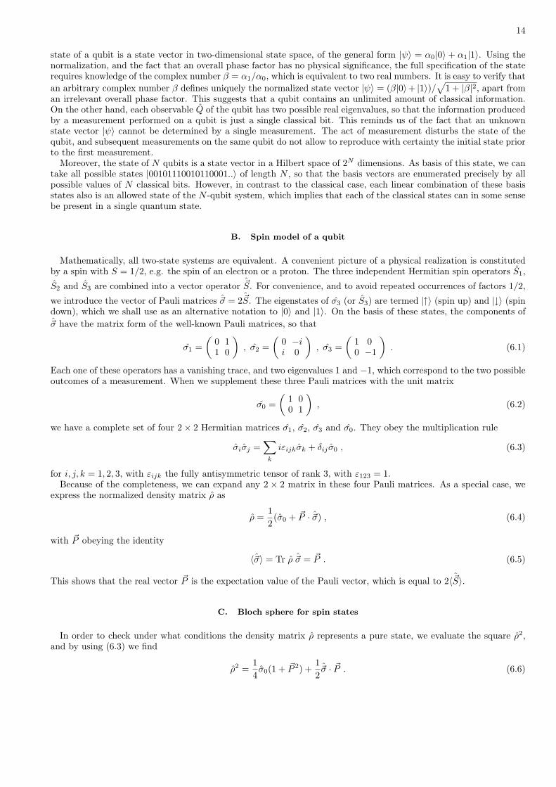
state of a qubit is a state vector in two-dimensional state space, of the general form |ψ〉 = α0|0〉 + α1|1〉. Using thenormalization, and the fact that an overall phase factor has no physical significance, the full specification of the staterequires knowledge of the complex number β = α1/α0, which is equivalent to two real numbers. It is easy to verify thatan arbitrary complex number β defines uniquely the normalized state vector |ψ〉 = (β|0〉+ |1〉)/

√1 + |β|2, apart from

an irrelevant overall phase factor. This suggests that a qubit contains an unlimited amount of classical information.On the other hand, each observable Q of the qubit has two possible real eigenvalues, so that the information producedby a measurement performed on a qubit is just a single classical bit. This reminds us of the fact that an unknownstate vector |ψ〉 cannot be determined by a single measurement. The act of measurement disturbs the state of thequbit, and subsequent measurements on the same qubit do not allow to reproduce with certainty the initial state priorto the first measurement.

Moreover, the state of N qubits is a state vector in a Hilbert space of 2N dimensions. As basis of this state, we cantake all possible states |00101110010110001..〉 of length N , so that the basis vectors are enumerated precisely by allpossible values of N classical bits. However, in contrast to the classical case, each linear combination of these basisstates also is an allowed state of the N -qubit system, which implies that each of the classical states can in some sensebe present in a single quantum state.

B. Spin model of a qubit

Mathematically, all two-state systems are equivalent. A convenient picture of a physical realization is constitutedby a spin with S = 1/2, e.g. the spin of an electron or a proton. The three independent Hermitian spin operators S1,

S2 and S3 are combined into a vector operator ~S. For convenience, and to avoid repeated occurrences of factors 1/2,

we introduce the vector of Pauli matrices ~σ = 2 ~S. The eigenstates of σ3 (or S3) are termed |↑〉 (spin up) and |↓〉 (spindown), which we shall use as an alternative notation to |0〉 and |1〉. On the basis of these states, the components of~σ have the matrix form of the well-known Pauli matrices, so that

σ1 =(

0 11 0

), σ2 =

(0 −ii 0

), σ3 =

(1 00 −1

). (6.1)

Each one of these operators has a vanishing trace, and two eigenvalues 1 and −1, which correspond to the two possibleoutcomes of a measurement. When we supplement these three Pauli matrices with the unit matrix

σ0 =(

1 00 1

), (6.2)

we have a complete set of four 2× 2 Hermitian matrices σ1, σ2, σ3 and σ0. They obey the multiplication rule

σiσj =∑

k

iεijkσk + δij σ0 , (6.3)

for i, j, k = 1, 2, 3, with εijk the fully antisymmetric tensor of rank 3, with ε123 = 1.Because of the completeness, we can expand any 2 × 2 matrix in these four Pauli matrices. As a special case, we

express the normalized density matrix ρ as

ρ =12(σ0 + ~P · ~σ) , (6.4)

with ~P obeying the identity

〈~σ〉 = Tr ρ ~σ = ~P . (6.5)

This shows that the real vector ~P is the expectation value of the Pauli vector, which is equal to 2〈 ~S〉.

C. Bloch sphere for spin states

In order to check under what conditions the density matrix ρ represents a pure state, we evaluate the square ρ2,and by using (6.3) we find

ρ2 =14σ0(1 + ~P 2) +

12~σ · ~P . (6.6)

15

As mentioned before, the density matrix (6.4) represents a pure state if and only if Tr ρ2 = 1, which is the case if thevector ~P has the length 1. Since for a pure state ρ has one eigenvalue 1, and one eigenvalue 0, the operator ~u · ~σ hasthe eigenvalues ±1 for all real unit vectors ~u. Since for a mixed state, the density matrix has two positive eigenvalues(that add up to 1), Eq. (6.4) represents a mixed state when the vector ~P has length |~P | < 1.

We conclude that the density matrix of a qubit can be uniquely represented by a point ~P in a sphere with radius 1.A mixed state corresponds to a vector ~P with |~P | < 1, which is represented by a point inside the sphere. The stateis pure when ~P = ~u is a unit vector, specified by a point on the surface of the unit sphere. This sphere is called theBloch sphere when the qubit is a spin 1/2. A pure-state vector is represented by a point on the surface of the Blochsphere, apart from an overall phase factor.

Now we consider a unit vector specified by the spherical angles θ and φ, so that ~u(θ, φ) = (cos φ sin θ, sin φ sin θ, cos θ),with 0 ≤ φ ≤ 2π, 0 ≤ θ ≤ π. We have seen that the operator ~u · ~σ has an eigenstate with eigenvalue 1, for which theexpectation value of the Pauli vector (or the spin vector) is directed parallel to ~u, and an eigenstate with eigenvalue−1, corresponding to a spin vector that is antiparallel to ~u. These eigenstates follow from the eigenstates |↑〉 and |↓〉after a rotation in spin space

R(θ, φ) = exp(−iφσ3/2) exp(−iθσ2/2) exp(iφσ3/2) . (6.7)

The operator R(θ, φ) consists of a rotation over an angle −φ about the 3-axis, then a rotation over an angle θ aboutthe 2-axis, and finally a rotation over an angle φ about the 3-axis. This rotation transforms the positive 3-directioninto the direction ~u. The matrix form of this rotations follows from the matrices for the rotations about the axes

exp(−iθσ2/2) =(

cos(θ/2) − sin(θ/2)sin(θ/2) cos(θ/2)

), exp(−iφσ3/2) =

(e−iφ/2 00 eiφ/2

). (6.8)

The eigenstate of ~u · ~σ with eigenvalue 1 is then

R(θ, φ)|↑〉 = cosθ

2|↑〉+ sin

θ

2eiφ|↓〉 . (6.9)

This is the pure state vector that is represented by the point ~u on the surface of the Bloch sphere. The opposite point−~u represents the state vector

R(θ, φ)|↓〉 = − sinθ

2e−iφ|↑〉+ cos

θ

2|↓〉 , (6.10)

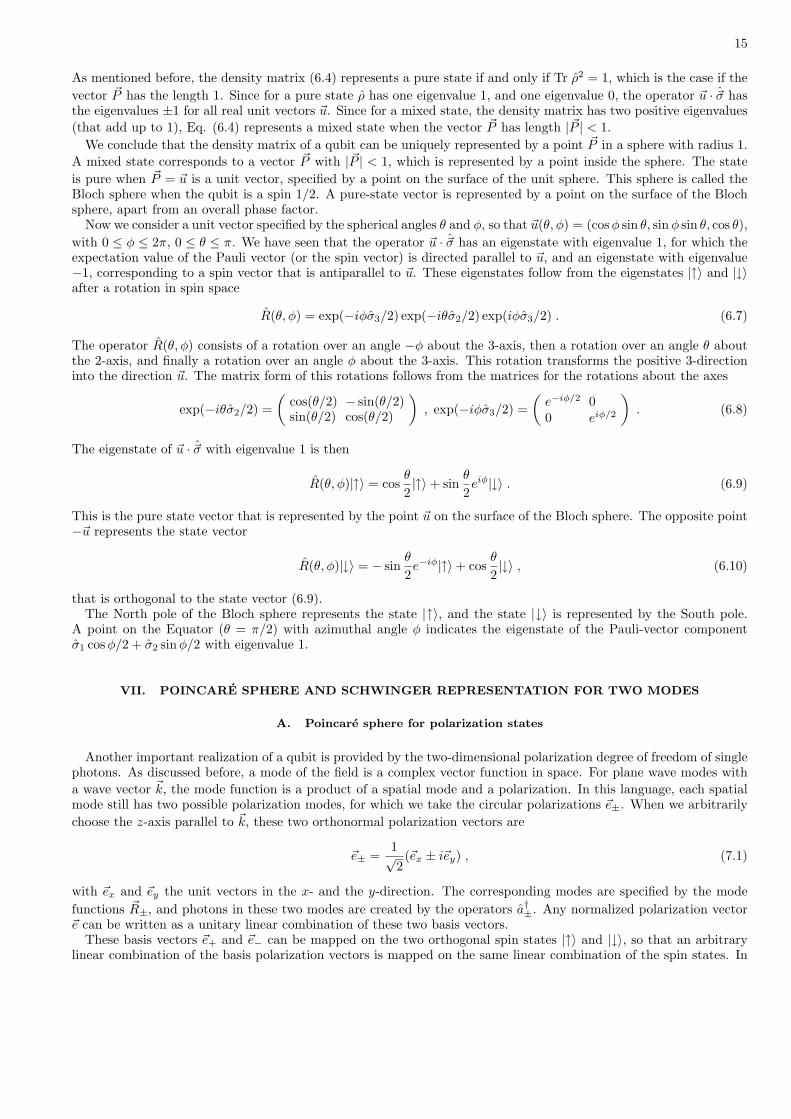
that is orthogonal to the state vector (6.9).The North pole of the Bloch sphere represents the state |↑〉, and the state |↓〉 is represented by the South pole.

A point on the Equator (θ = π/2) with azimuthal angle φ indicates the eigenstate of the Pauli-vector componentσ1 cos φ/2 + σ2 sinφ/2 with eigenvalue 1.

VII. POINCARE SPHERE AND SCHWINGER REPRESENTATION FOR TWO MODES

A. Poincare sphere for polarization states

Another important realization of a qubit is provided by the two-dimensional polarization degree of freedom of singlephotons. As discussed before, a mode of the field is a complex vector function in space. For plane wave modes witha wave vector ~k, the mode function is a product of a spatial mode and a polarization. In this language, each spatialmode still has two possible polarization modes, for which we take the circular polarizations ~e±. When we arbitrarilychoose the z-axis parallel to ~k, these two orthonormal polarization vectors are

~e± =1√2(~ex ± i~ey) , (7.1)

with ~ex and ~ey the unit vectors in the x- and the y-direction. The corresponding modes are specified by the modefunctions ~R±, and photons in these two modes are created by the operators a†±. Any normalized polarization vector~e can be written as a unitary linear combination of these two basis vectors.

These basis vectors ~e+ and ~e− can be mapped on the two orthogonal spin states |↑〉 and |↓〉, so that an arbitrarylinear combination of the basis polarization vectors is mapped on the same linear combination of the spin states. In

16

this way, the two-dimensional space of polarization vectors is represented as points on the surface of the unit sphere.The sphere representing polarization vectors is termed the Poincare sphere [8]. Then the point on the Poincare spherewith the spherical angles θ and φ represents the polarization vector

~eup(θ, φ) = ~e+ cosθ

2+ ~e− sin

θ

2eiφ , (7.2)

in analogy to the spin state (6.9). An alternative expression for the same polarization vector is obtained by separating(7.2) as ~eup(θ, φ) = exp(iφ/2) (~eR(θ, φ) + i~eI(θ, φ)), with

~eR(θ, φ) =1√2

(cos

θ

2+ sin

θ

2

)(~ex cos

φ

2+ ~ey sin

φ

2

),

~eI(θ, φ) =1√2

(cos

θ

2− sin

θ

2

)(−~ex sin

φ

2+ ~ey cos

φ

2

). (7.3)

Since ~eR and ~eI are orthogonal, it is easy to recognize the shape of the polarization ellipse. Since ~eI is smaller than~eR (except at the poles), the direction of ~eR indicates the long axis of the ellipse. The North pole of the Poincaresphere represents right circular polarization ~e+, the South pole represents left circular polarization ~e−. The pointon the Equator (θ = π/2) with azimuthal angle φ specifies linear polarization at an angle φ/2 with the x-axis. Inbetween the poles and the Equator, the polarization is elliptical. Opposite points on the sphere represent orthogonalpolarizations. The polarization corresponding to the opposite spin state (6.10) is equal to

~edown(θ, φ) = −~e+ sinθ

2e−iφ + ~e− cos

θ

2. (7.4)

We consider now the two modes with mode functions ~R±, which have the same spatial behavior (ideally a planewave with wave vector ~k = k~ez), and opposite circular polarization ~e±. The two-dimensional one-photon state space isspanned by the basis set a†±|0, 0〉, with |0, 0〉 the two-mode vacuum state. The one-photon state with the polarization(7.2) is then obtained as the corresponding linear combination of these basis states, and the same is true for theone-photon state with the opposite polarization (7.4). These states result when the creation operators

a†(θ, φ) = a†+ cosθ

2+ a†− sin

θ

2eiφ , b†(θ, φ) = −a†+ sin

θ

2e−iφ + a†− cos

θ

2(7.5)

act on the vacuum state. Hence, the operators (7.5) create a photon with polarization ~eup(θ, φ) or ~edown(θ, φ). Eachone-photon state in these two modes is uniquely represented by a point on the surface of the unit sphere. A mixedstate, represented as a 2× 2 density matrix on these basis states is represented by a real vector ~P inside the Poincaresphere, in full analogy to the Bloch sphere representing density matrices of a spin 1/2.

B. Stokes operators

In the case of a spin 1/2, the three directions 1, 2 and 3 and the points on the Bloch sphere indicate the componentsof the spin vector along the x, y and z axes in real space. In the case of polarization, the space of the Pauli operatorsand the points on the Poincare sphere refer to a fictitious space, that is defined in mere analogy to the spin case. Thethree components of the unit vector ~u = (u1, u2, u3) correspond respectively to the degree of linear polarization alongthe x and the y axis (u1), the degree of linear polarization in the directions under 45 with the x- and the y-axis(u2), and the degree of circular polarization (u3). This can be checked from the significance of the vector ~u as theexpectation value of the Pauli vector ~σ. In classical optics these quantities are known as the Stokes parameters, thattogether fully specify the polarization vector [8].

From the Bloch-Poincare analogy we know that for an arbitrary one-photon state a†(θ, φ)|0, 0〉, the expectationvalue of the Pauli vector is 〈~σ〉 = ~u, where the Pauli operators have the form of the Pauli matrices on the basis ofthe states a†±|0, 0〉. Similarly, when a density matrix ρ on this two-dimensional state space of one-photon states takesthe form (6.4), the expectation value is 〈~σ〉 = ~P , and the density matrix can be uniquely represented by the point ~Pinside the Poincare sphere.

Within the two-dimensional state space of one-photon states the action of the Pauli operators σ1, σ2 and σ3 coincides

with the action of the operators ~Σ, defined by the three components

Σ1 = a†−a+ + a†+a− ,

17

Σ2 = ia†−a+ − ia†+a− ,

Σ3 = a†+a+ − a†−a− , (7.6)

which can be summarized in an elegant fashion by the notation

~Σ = (a†+ a†−)~σ(

a+

a−

)(7.7)

The operators Σ1/2, Σ2/2 and Σ3/2 obey the commutation rule of angular momentum operators, just as the spinoperators S1 = σ1/2, S2 = σ2/2 and S3 = σ3/2. On the other hand, these operators obviously are defined on arbitrarystates of the system consisting of the two modes ~R±, not just the one-photon states. These operators play the roleof the Stokes operators, which may be regarded as a quantum version of the classical Stokes vector that specifies thepolarization state of a beam of light [8].

The operators ~Σ conserve the number of photons, and thereby commute with the total photon number Σ0 =N+ + N− = a†+a+ + a†−a−. The quantum version of the Stokes vector is the vector ~P , defined by its components

Pi =〈Σi〉〈Σ0〉

, (7.8)

with i = 1, 2, 3. For the case of one-photon states, the denominator is always equal to 1, so that this definitioncoincides with the earlier definition in this special case. Only then does the vector ~P determine the density matrixcompletely. In the N +1-dimensional subspace of N photons, specification of the full density matrix requires N2 +2N

parameters, with the vector ~P , defined by (7.8) specifying 3 of them.

C. Schwinger representation of two modes

We have noticed that the three operators ~Σ/2 behave as the components of an angular momentum. This is thebasis of the Schwinger representation, which builds on the equivalence of the 2J + 1-dimensional state space of anangular momentum J with the states of two boson modes with total boson number N = 2J [9]. The eigenstate |JM〉of J3 with eigenvalue M corresponds to the eigenstate |n+, n−〉 = |n+, N − n+〉 of Σ3/2 with M = (n+ − n−)/2. Itis interesting to notice that the spin angular momentum of the photon state is equal to (n+ − n−)~ = 2M~. Thisreminds us of the fact that, in contrast to the Bloch sphere, the Poincare sphere does not generally specify the angularmomentum vector of the state of the two modes.

The components of the angular-momentum operator are Ji = Σi/2. The representation of the rotation group SU(2)with dimension 2J + 1 = N + 1 is generated by the N -boson states. The rotation corresponding to Eq. (6.7) in thetwo-mode space takes the form

R(θ, φ) = exp(−iφΣ3/2) exp(−iθΣ2/2) exp(iφΣ3/2) = exp(−iφJ3) exp(−iθJ2) exp(iφJ3) . (7.9)

This rotation operator acting on one-photon states with polarizations ~e± transforms these into the polarizations~eup(θ, φ) and ~edown(θ, φ). This corresponds to the rotation transformations of the creation operators a†± into theoperators (7.5), as expressed by

R(θ, φ)a†+R†(θ, φ) = a†(θ, φ) , R(θ, φ)a†−R†(θ, φ) = b†(θ, φ) . (7.10)

The same rotation operator transforms the circularly polarized N -photon state |N, 0〉 into an N -photon state withpure polarization at the point ~u(θ, φ) on the Poincare sphere:

R(θ, φ)|N, 0〉 =1√N !

R(θ, φ)(a†+)N |0, 0〉 =1√N !

(a†(θ, φ))N |0, 0〉 (7.11)

In the angular-momentum language, this is the state vector with maximal angular momentum in the direction ~u(θ, φ).In analogy to the coherent states of a mode of the radiation field, it is commonly termed a spin-coherent state [10].Just as a coherent state (4.6) is a displaced version of the vacuum state, the spin coherent state is a rotated versionof the state with maximal angular momentum along the 3-axis. This analogy is particularly clear when we rewritethe rotation operator (7.9) as

exp(−iφJ3) exp(−iθJ2) exp(iφJ3) = exp[−iθ(J2 cos φ− J1 sin φ)] = exp(zJ− − z∗J+) , (7.12)

with z = (θ/2) exp(iφ). Here we denoted as usual J± = J1 ± iJ2. Note the similarity between the rotation operator(7.12) and the displacement operator (4.7), with J+ playing the part of a, and J− of a†.

18

VIII. ANGULAR MOMENTUM OF MONOCHROMATIC PARAXIAL BEAMS

A. Paraxial approximation

The paraxial approximation for the radiation field applies when the wave vectors of the field fall within a narrow conewith a small opening angle. This is the case for light beams, as they are produced by lasers. In this approximation theelectric field of a light beam with frequency ω that propagates in vacuum in the positive z-direction can be expressedas the product of a plane wave and a slowly-varying envelope. The components of ~E in the transverse (x, y)-planecan be expressed as

~Et (~r, t) = ~u(ρ, z)ei(kz−ωt) + c.c. , (8.1)

with ω = ck. Here ρ = (x, y) is the 2D transverse position vector and ~r = (ρ, z) is the position vector in threedimensions. The propagation equation for ~u follows from the Helmholtz equation ~∇2 ~E = −k2 ~E for the electric field.The paraxial approximation is justified when |∂u/∂ρ|/(ku) ¿ 1. In that case the transverse profile of ~u varies onlyslowly with z, so that the second derivative with respect to z can be ignored. Then the propagation of the light beamis well described by the paraxial wave equation [11, 12]

(∇2

ρ + 2ik∂

∂z

)~u(ρ, z) = 0 , (8.2)

where ∇ρ is the gradient operator in the transverse direction. The vector field ~u lies in the transverse (xy) plane.The paraxial approximation can be viewed as a lowest-order term of an expansion in the small paraxial parameterδ = 1/(kγ0), with γ0 the beam waist [11]. The magnetic field in the transverse plane is

~Bt (~r, t) =1c~ez × ~u(ρ, z)ei(kz−ωt) + c.c. , (8.3)

Equation (8.3) shows that the components of the magnetic field in the transverse plane has the same pattern as theelectric field, with a polarization that is equal to the electric polarization vector rotated over an angle π/2 in thepositive (anti-clockwise) direction.

The z-components of the fields ~E and ~B are non-vanishing in higher order. Since both fields are divergence-free,their first-order terms are proportional to the transverse divergence of ~Et and ~Bt, and we find

Ez =i

k∇ρ · ~u ei(kz−ωt) + c.c. , Bz =

i

k∇ρ · (~ez × ~u) ei(kz−ωt) + c.c. . (8.4)

B. Angular momentum of monochromatic beam

The momentum density has a leading term ε0 ~Et × ~Bt, which points in the z-direction. After using the expressions(8.1) and (8.3), and eliminating the rapidly oscillating terms by averaging over a few optical cycles, the zeroth-ordercontribution to the momentum density is found as

pz(~R, z) =2ε0c

~u∗ · ~u . (8.5)

It is easy to verify that the leading term in the Poynting vector ~S = ~E× ~H is equal to its z-component Sz = c2pz = cw,with

w(~R, z) =12ε0

(~E2

t + c2 ~B2t

)= 2ε0~u

∗ · ~u (8.6)

the energy density of the beam. When we use the photon energy ~ω as an energy quantum, the photon density isn = w/(~ω), and the momentum density (8.5) amounts to n~k, which corresponds to ~k per photon. The energy perunit length is denoted as

W =∫

d2ρ w(ρ, z) = 2ε0

∫d2ρ u∗ · u . (8.7)

19

However, we are not interested in the angular momentum arising from this photon momentum along the axis, butin the component jz of the angular-momentum density in the propagation direction. Since

jz = ρ× ~pt , (8.8)

this z-component arises from the components of the momentum density in the transverse (xy) plane. To first orderin δ, the transverse component of the momentum density is

~pt = ε0

[Ez(~ez × ~Bt) + ( ~Et × ~ez)Bz

]. (8.9)

After substituting the expressions (8.1), (8.3) and (8.4), and averaging over an optical cycle, one finds that jz can beseparated into the sum jz = l + s, where l and s are given by the expressions in cylindrical coordinates

l(ρ, z) =ε0iω

~u∗ · ∂

∂φ~u + c.c. , s(ρ, z) = − ε0

iωρ

∂

∂ρ(~u∗ × ~u) . (8.10)

The contribution l is determined by the phase gradient of the two components of ~u in the azimuthal direction. Thisexpression has the flavor of a density of orbital angular momentum, as is obvious when we compare it to the expressionfor the z-component of the orbital angular momentum of a particle in elementary quantum mechanics. The separationof jz in l and s holds exactly for the contributions to the density of angular momentum. The quantity s arises from thegradient in the radial direction of the cross product (~u∗ × ~u) /i of the transverse mode amplitude. We recall that foran arbitrary radiation field, the separation (3.2) of ~J into ~L and ~S could only be made for the total angular momenta,integrated over the entire space. It is remarkable that for a paraxial beam the separation of jz as l + s arises for thedensities, in each point of space separately. Even so, the expression (8.10) for l is identical to the z-component of theintegrand in the expression (3.3) for ~L, when ~A and ~E⊥ are represented by their monochromatic paraxial expressions.

The spin per unit beam length is given by the integral Σ ≡ ∫dρ s(ρ, z), and the orbital angular momentum per

unit length is equal to Λ ≡ ∫dρ l(ρ, z). We use partial integration with respect to φ for Λ, and with respect to ρ for

Σ, and we obtain

Λ =2ε0ω

∫d2ρ ~u∗ · 1

i

∂

∂φ~u , Σ =

2ε0ω

∫d2ρ (~u∗ × ~u) /i . (8.11)

It is easy to show that both Σ and Λ do not vary with the propagation coordinate z under free propagation [13]. Onealso easily verifies that the integrand of this expression for Σ coincides with the integrand in (3.3) for the z-componentof ~S. Again, this is remarkable, since the integration in (8.11) runs only over the transverse plane, not over the entirevolume.

When we separate the complex vector field ~u(ρ, z) as ~u = u~e, with ~e the complex normalized local polarizationvector, and u = |~u| the local field strength, we arrive at the identity 2ε0 (~u∗ × ~u) /i = σw, where the cross productσ = (~e∗ × ~e) /i is the local helicity of the beam. The helicity σ is a real number that is zero for linear polarization,and it takes the value ±1 for circular polarization ~e± = (~ex ± i~ey)/

√2. The spin density in (8.10) is found to be

localized in the region of the radial gradient of the product σw. However, equation (8.11) for Σ may be read as anintegration of n~σ, which is the product of the photon density n = w/(~ω) and the spin ~σ per photon, where boththe photon density and the helicity may depend on the transverse position ρ.

C. Uniform orbital and spin angular momentum

The expressions (8.10) and (8.11) generalize the results for a monochromatic beam with uniform polarization. Inthat case, we can write ~u(ρ, z) = ~eu(ρ, z), where the polarization vector ~e is independent of position. Then the helicityσ is uniform over the cross section of the beam, and we recover from Eqs. (8.10) the known expressions [14]

l(ρ, z) =ε0iω

u∗∂

∂φu + c.c. , s(ρ, z) = − σ

2ωρ

∂

∂ρw(ρ, z) . (8.12)

This shows that the spin density is determined by the radial derivative of the energy density. The integrated spinmomentum obeys the relation Σ = σW/ω, which corresponds to ~σ per photon, as expected [15]. However, the spin islocalized in the region of the gradient of energy density, so that it vanishes in the region of uniform intensity. On theother hand, when a fraction of the light is absorbed by a particle, or when it is cut out by an aperture, the relationΣ = σW/ω also applies for this fraction. In this sense it is justified to say that light with a uniform helicity σ carriesa spin ~σ per photon [16].

20

Of special interest are mode profiles of the form

u(ρ, φ, z) = Fm(ρ, z) exp(imφ) , (8.13)

where the φ-dependence is given by the factor exp(imφ). In order that the mode is continuous, m must be an integer.Then the density of orbital angular momentum is equal to l = mw/ω = n~m, and the orbital angular momentumper photon is ~m. They are eigenmodes of the differential operator ∂/∂φ. However, it would be confusing to statethat they are eigenmodes of orbital angular momentum. In the classical context we are discussing here, orbitalangular momentum is just a classical quantity, not an operator. For any classical beam the amount of orbital angularmomentum has a well-defined specific value, and the same is true for the spin. What is special about these modes isthat the density of orbital angular momentum is proportional to the energy density. In this sense, the orbital angularmomentum can be said to be uniform over the beam profile. The modes (8.13) have an orbital angular momentumthat can be quantified as ~m per photon. Since the paraxial wave equation (8.2) is isotropic, this φ-dependence isconserved during free propagation. The radial mode function Fm obeys the radial paraxial wave equation

(∂2

∂ρ2+

1ρ

∂

∂ρ− m2

ρ2+ 2ik

∂

∂z

)Fm(ρ, z) = 0 . (8.14)

A well-known example is provided by the Laguerre-Gaussian modes [14, 17]. For these modes the radial modefunctions are denoted as Fmp(ρ, z), where p is the radial mode number. The real function Fmp is the product of aGaussian function, a factor ρ|m|, and an associated Laguerre polynomial that depends only on the absolute value|m| [17]. These mode functions have the special property that their radial shape is invariant during free propagation,apart from a scaling factor. The z-dependent scaling factor is the width of the radial profile. Around the beam axis,the profiles of these beams are proportional to ρ|m| exp(imφ) = (x± iy)|m|, depending on the sign of m. This showsthat the beams have a phase singularity which corresponds to a vortex of charge m.

D. Non-uniform polarization

When a beam with non-uniform polarization passes a polarizer, the mode profile of the outgoing beam depends onthe setting of the polarizer. This means that the mode function ~u does not factorize into the form ~eu(ρ, z), with afixed polarization vector. On the quantum level, this means that for each photon in the beam its polarization and itstranslational degrees of freedom are entangled. At present, light beams with a non-uniform linear polarization andaxial symmetry are widely studied. They can be generated by spatially varying dielectric gratings [18, 19].

As an example, we consider the superposition of two Laguerre-Gaussian light beams with opposite azimuthal modenumber ±m, and with opposite circular polarizations. We consider a monochromatic beam characterized by the modepattern

~u(ρ, φ, z) = Fmp(ρ, z)[~e+e−imφ + ~e−eimφ

]/√

2 . (8.15)

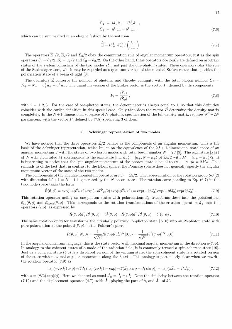
The mode function (8.15) is real everywhere, and it is the superposition of two components with orbital angularmomentum per photon ∓m~, and spin ±~ per photon. The vector multiplying Fmp in Eq. (8.15) is a φ-dependentlinear polarization vector ~e(φ) = ~ex cos(mφ) + ~ey sin(mφ). This polarization vector is in the x direction for φ = 0,and along a circle around the beam axis the polarization direction makes m full rotations in the positive direction.The directions of linear polarization as a function of φ are indicated by the black arrows in Figure 3. The linearlypolarized field oscillates in phase everywhere along such a circle. For negative values of m, the polarization directionrotates in the negative direction along the circle.

In the special case that m = 1, the number of rotations is 1, and the pattern is rotationally invariant. Thenthe density of angular momentum jz = l + s is zero, and the beam is invariant for rotation around the axis. Thepolarization direction is always in the radial direction. When we replace φ by φ− φ0 in the right-hand side of (8.15),the pattern is still isotropic, and the polarization direction makes an angle φ0 with the radial direction.

The density of orbital and spin angular momentum of the mode (8.15) can be evaluated with equation (8.10), andare both found to be zero. In fact, this mode is a superposition of two terms with orbital angular momentum equalto ∓~m, and spin ±~ per photon. The energy density is

w(ρ, z) = 2ε0|Fmp(ρ, z)|2 . (8.16)

Accordingly, near the axis, the pattern of phase and polarization is described by the expression

~u(x, y) ∝ (~ex + i~ey)(x− iy)m + (~ex + i~ey)(x + iy)m . (8.17)

21

m=1 m=2

m=-1 m=-2

FIG. 3: Sketch of the position-dependent linear polarization for a mode as described by Eq. (8.15). The arrows indicate thedirection of the linear polarization.

This describes a singularity in phase and polarization with a mixed charge.An interesting generalization is the case of a similar superposition of modes with opposite circular polarization, and

φ-dependent phase terms with two arbitrary m-values. This gives a transverse mode function

~u(ρ, φ) = F (ρ)[~e+eim′φ + ~e−eimφ

]/√

2 , (8.18)

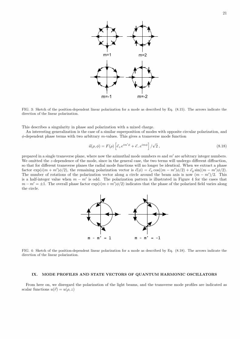
prepared in a single transverse plane, where now the azimuthal mode numbers m and m′ are arbitrary integer numbers.We omitted the z-dependence of the mode, since in the general case, the two terms will undergo different diffraction,so that for different transverse planes the radial mode functions will no longer be identical. When we extract a phasefactor exp(i(m + m′)φ/2), the remaining polarization vector is ~e(φ) = ~ex cos((m − m′)φ/2) + ~ey sin((m − m′)φ/2).The number of rotations of the polarization vector along a circle around the beam axis is now (m − m′)/2. Thisis a half-integer value when m − m′ is odd. The polarization pattern is illustrated in Figure 4 for the cases thatm−m′ = ±1. The overall phase factor exp(i(m + m′)φ/2) indicates that the phase of the polarized field varies alongthe circle.

m - m’ = 1 m - m’ = -1

FIG. 4: Sketch of the position-dependent linear polarization for a mode as described by Eq. (8.18). The arrows indicate thedirection of the linear polarization.

IX. MODE PROFILES AND STATE VECTORS OF QUANTUM HARMONIC OSCILLATORS

From here on, we disregard the polarization of the light beams, and the transverse mode profiles are indicated asscalar functions u(~r) = u(ρ, z)

22

A. Paraxial beams and quantum harmonic oscillators

It is well-known that the paraxial wave equation has a complete set of solutions in the form of a Gaussian functionmultiplied by a Hermite polynomial [17]. These Hermite-Gaussian mode functions have an intensity pattern thatis invariant under propagation, apart from a scaling factor. They closely resemble the eigenfunctions of the two-dimensional quantum harmonic oscillator (HO). In fact, the Hermite-Gaussian mode functions can be written as [20]

unxny(~r) =

1γ

ψnx

(x

γ

)ψny

(y

γ

)exp

(ikρ2

2R− iχ(nx + ny + 1)

). (9.1)

These mode functions are determined by three mode parameters that depend on the propagation coordinate z. Thewidth γ determines the spot size, R is the radius of curvature of the wave fronts, and χ is the Gouy phase, thatdetermines the phase delay over the beam focus. When the transverse plane z = 0 coincides with the focal plane, thez-dependence of these parameters is determined by the equalities

1γ(z)2

− ik

R(z)=

k

b + iz, tan χ(z) =

z

b. (9.2)

Here b is the diffraction length (or Rayleigh range) of the beam. The Gouy phase increases by an amount π fromz = −∞ to ∞. The mode functions (9.1) are exact normalized solutions of the paraxial wave equation (8.2).The spot size at focus is γ0 = γ(0) =

√b/k. Here the functions ψn(ξ) for n = 0, 1, . . . are the real normalized

energy eigenfunctions of the one-dimensional quantum harmonic oscillator in dimensionless form. Hence they areeigenfunctions of the Hamiltonian

Hξ =12

(− ∂2

∂ξ2+ ξ2

)(9.3)

with eigenvalue n + 1/2. The explicit form of the normalized eigenfunctions is

ψn(ξ) =1√

2nn!√

πe−ξ2/2Hn(ξ) , (9.4)

in terms of the Hermite polynomials Hn, and the eigenvalues are n + 1/2.The Gouy phase term in the Hermite-Gaussian modes (9.1) is proportional to the eigenvalue nx + ny + 1 of the

Hamiltonian of the two-dimensional quantum harmonic oscillator. This allows us to express an arbitrary solutionof the paraxial wave equation in terms of an arbitrary time-dependent solution of the Schrodinger equation of theharmonic oscillator, provided that we replace time by the Gouy phase χ. In dimensionless notation, this equationtakes the form

∂

∂χΨ(ξ, η, χ) = −i

(Hξ + Hη

)Ψ(ξ, η, χ) . (9.5)

Obviously, wave functions ψnx(ξ)ψny (η) exp(−i(nx + ny + 1)χ) are solutions of this Schrodinger equation, and bytaking linear combination of these one obtains the most general solution Ψ(ξ, η, χ). On the other hand, an arbitrarysolution of the paraxial wave equation is a linear combination of the Hermite-Gaussian modes (9.1). We concludethat an arbitrary solution Ψ(ξ, η, χ) of (9.5) gives an arbitrary solution u(~r) of (8.2), by the identification [21]

u(~r) =1γ

Ψ(ξ, η, χ) exp(

ikρ2

2R(z)

), (9.6)

with ξ = x/γ, η = y/γ, and where the z-dependent parameters γ, R and χ are specified by Eq. (9.2) as functions ofz.

This identification (9.6) is exact, and it works both ways: there is a one-to-one correspondence between a time-dependent state of the two-dimensional harmonic oscillator and a monochromatic paraxial beam of light. For a givenharmonic oscillator wave function, we find a mode function after choosing as free parameter the diffraction length b,which is a measure of the size of the focal region. Moreover, a solution of the quantum harmonic oscillator remains asolution under a shift of time. If we substitute in (9.6) Ψ(ξ, η, χ−χ0) for Ψ(ξ, η, χ), we find a different paraxial beamin general. For an arbitrary mode, a phase shift χ0 = π/2 leads to an interchange of the mode pattern in focus and inthe far field. Since the Gouy phase increases by an amount π, the mode function u from z = −∞ to ∞ correspondsto half a cycle of the oscillator.

A stationary state of the harmonic oscillator is a linear superposition of products ψnx(ξ)ψny (η) with nx + ny = nconstant. Then Ψ(ξ, η, χ) is proportional to exp(−i(nx + ny + χ)), and the corresponding paraxial beam retains itsshape during propagation, apart from scaling by the width γ(z) and the z-dependent radius of curvature R(z).

23

B. Dirac notation of a paraxial beams

As is well-known, the paraxial wave equation (8.2) for a monochromatic beam is mathematically equivalent to theSchrodinger equation of a free quantum particle in two dimensions, where the propagation coordinate z replaces time.This analogy suggests to denote the mode function ~u as a function of ρ in a single transverse plane as a state vector|~u(z)〉 in Dirac notation [22], so that u(ρ, z) = 〈ρ|u(z)〉. The scalar product of two state vectors

〈v|u〉 =∫

d2ρ v∗(ρ) · u(ρ) (9.7)

involves an integration over the transverse coordinates. The relation between quantum and classical mechanics isanalogous to the relation between paraxial wave optics and ray optics. A ray that passes a transverse plane iscompletely determined by its position ρ, and the 2-vector θ = (θx, θy) of direction angles. The direction angles arethe ratio between the transverse momentum and the longitudinal momentum ~k, and the operators for the directionangles therefore take the form θ = (θx, θy) = −(i/k)∇ρ. The paraxial wave equation (8.2) can be written as

∂

∂z|u(z)〉 = − ik

2θ2|u(z)〉 . (9.8)

The effect on a state vector of free propagation over a distance L is then described by the operator

Uprop(L) = exp(− ik

2θ2L

). (9.9)

The position operators ρ and the direction operators θ are both Hermitian, and they obey the commutation rules

[ρa, kθb] = iδab , (9.10)

where the indices a and b run over the x and y components.It is convenient to work with mode functions that are normalized to 1, so that

〈u|u〉 = 〈Ψ|Ψ〉 = 1 . (9.11)

Then the orbital angular momentum per photon along the beam axis of a monochromatic beam as given in (8.11) is

~ωΛW

= ~k〈u|ρ× θ|u〉 = 〈u|~i

∂

∂φ|u〉 = 〈Ψ|~

i

∂

∂φ|Ψ〉 , (9.12)

with Λ and W the orbital angular momentum and the energy per unit length. This expression (9.12) resembles thatfor the orbital angular momentum of a quantum particle in two dimensions.

We emphasize that although the operator notation is borrowed from quantum mechanics, the description is appliedhere to classical paraxial optics.

C. Raising and lowering operators for a paraxial beam

As is well-known from textbook quantum mechanics, the eigenstates of the quantum harmonic oscillator are linkedby ladder operators that raise or lower the quantum number n. In dimensionless notation, the lowering operator for thewave function ψn(ξ) takes the form a = (ξ + ∂/∂ξ)/

√2. This formalism can be carried over to the Hermite-Gaussian

modes |unxny (z)〉, so that these modes are linked to the fundamental mode |u00(z)〉 by the standard relation

|unxny (z)〉 =1√

nx!ny!

(a†x(z)

)nx(a†y(z)

)ny |u00(z)〉 . (9.13)

The Hermite-Gaussian modes factorize into a product of a function of x and a function of y. They do not have vortexstructures, but only contain line dislocations, with opposite phases on opposite sides of the lines.

In terms of the canonical operators ρ and θ the ladder operators take the form [20]

ax(z) =

√k

2b

(x + i(b + iz)θx

), ay(z) =

√k

2b

(y + i(b + iz)θy

). (9.14)

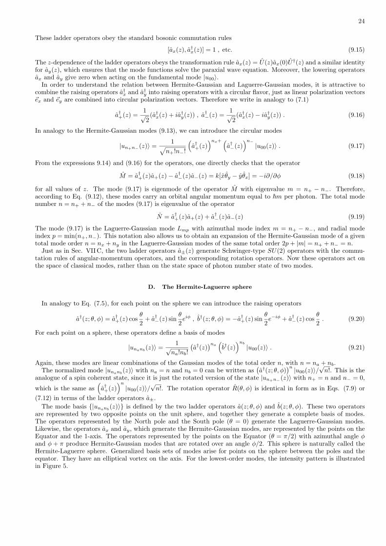
24

These ladder operators obey the standard bosonic commutation rules

[ax(z), a†x(z)] = 1 , etc. (9.15)

The z-dependence of the ladder operators obeys the transformation rule ax(z) = U(z)ax(0)U†(z) and a similar identityfor ay(z), which ensures that the mode functions solve the paraxial wave equation. Moreover, the lowering operatorsax and ay give zero when acting on the fundamental mode |u00〉.

In order to understand the relation between Hermite-Gaussian and Laguerre-Gaussian modes, it is attractive tocombine the raising operators a†x and a†y into raising operators with a circular flavor, just as linear polarization vectors~ex and ~ey are combined into circular polarization vectors. Therefore we write in analogy to (7.1)

a†+(z) =1√2(a†x(z) + ia†y(z)) , a†−(z) =

1√2(a†x(z)− ia†y(z)) . (9.16)

In analogy to the Hermite-Gaussian modes (9.13), we can introduce the circular modes

|un+n−(z)〉 =1√

n+!n−!

(a†+(z)

)nx+ (a†−(z)

)n− |u00(z)〉 . (9.17)

From the expressions 9.14) and (9.16) for the operators, one directly checks that the operator

M = a†+(z)a+(z)− a†−(z)a−(z) = k[xθy − yθx] = −i∂/∂φ (9.18)

for all values of z. The mode (9.17) is eigenmode of the operator M with eigenvalue m = n+ − n−. Therefore,according to Eq. (9.12), these modes carry an orbital angular momentum equal to ~m per photon. The total modenumber n = n+ + n− of the modes (9.17) is eigenvalue of the operator

N = a†+(z)a+(z) + a†−(z)a−(z) (9.19)

The mode (9.17) is the Laguerre-Gaussian mode Lmp with azimuthal mode index m = n+ − n−, and radial modeindex p = min(n+, n−). This notation also allows us to obtain an expansion of the Hermite-Gaussian mode of a giventotal mode order n = nx + ny in the Laguerre-Gaussian modes of the same total order 2p + |m| = n+ + n− = n.

Just as in Sec. VII C, the two ladder operators a±(z) generate Schwinger-type SU(2) operators with the commu-tation rules of angular-momentum operators, and the corresponding rotation operators. Now these operators act onthe space of classical modes, rather than on the state space of photon number state of two modes.

D. The Hermite-Laguerre sphere

In analogy to Eq. (7.5), for each point on the sphere we can introduce the raising operators

a†(z; θ, φ) = a†+(z) cosθ

2+ a†−(z) sin

θ

2eiφ , b†(z; θ, φ) = −a†+(z) sin

θ

2e−iφ + a†−(z) cos

θ

2. (9.20)

For each point on a sphere, these operators define a basis of modes

|unanb(z)〉 =

1√na!nb!

(a†(z)

)na(b†(z)

)nb |u00(z)〉 . (9.21)

Again, these modes are linear combinations of the Gaussian modes of the total order n, with n = na + nb.The normalized mode |unanb

(z)〉 with na = n and nb = 0 can be written as(a†(z; θ, φ)

)n |u00(z)〉/√

n!. This is theanalogue of a spin coherent state, since it is just the rotated version of the state |un+n−(z)〉 with n+ = n and n− = 0,

which is the same as(a†+(z)

)n

|u00(z)〉/√

n!. The rotation operator R(θ, φ) is identical in form as in Eqs. (7.9) or(7.12) in terms of the ladder operators a±.

The mode basis |unanb(z)〉 is defined by the two ladder operators a(z; θ, φ) and b(z; θ, φ). These two operators

are represented by two opposite points on the unit sphere, and together they generate a complete basis of modes.The operators represented by the North pole and the South pole (θ = 0) generate the Laguerre-Gaussian modes.Likewise, the operators ax and ay, which generate the Hermite-Gaussian modes, are represented by the points on theEquator and the 1-axis. The operators represented by the points on the Equator (θ = π/2) with azimuthal angle φand φ + π produce Hermite-Gaussian modes that are rotated over an angle φ/2. This sphere is naturally called theHermite-Laguerre sphere. Generalized basis sets of modes arise for points on the sphere between the poles and theequator. They have an elliptical vortex on the axis. For the lowest-order modes, the intensity pattern is illustratedin Figure 5.

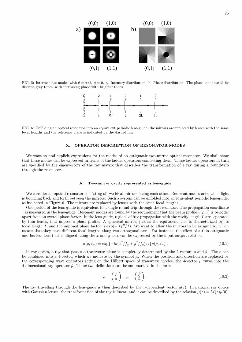
25

FIG. 5: Intermediate modes with θ = π/3, φ = 0. a. Intensity distribution. b. Phase distribution. The phase is indicated bydiscrete grey tones, with increasing phase with brighter tones.

FIG. 6: Unfolding an optical resonator into an equivalent periodic lens-guide; the mirrors are replaced by lenses with the samefocal lengths and the reference plane is indicated by the dashed line.

X. OPERATOR DESCRIPTION OF RESONATOR MODES

We want to find explicit expressions for the modes of an astigmatic two-mirror optical resonator. We shall showthat these modes can be expressed in terms of the ladder operators connecting them. These ladder operators in turnare specified by the eigenvectors of the ray matrix that describes the transformation of a ray during a round-tripthrough the resonator.

A. Two-mirror cavity represented as lens-guide

We consider an optical resonator consisting of two ideal mirrors facing each other. Resonant modes arise when lightis bouncing back and forth between the mirrors. Such a system can be unfolded into an equivalent periodic lens-guide,as indicated in Figure 6. The mirrors are replaced by lenses with the same focal lengths.

One period of the lens-guide is equivalent to a single round-trip through the resonator. The propagation coordinatez is measured in the lens-guide. Resonant modes are found by the requirement that the beam profile u(ρ, z) is periodicapart from an overall phase factor. In the lens-guide, regions of free propagation with the cavity length L are separatedby thin lenses, that impose a phase profile. A spherical mirror, just as the equivalent lens, is characterized by itsfocal length f , and the imposed phase factor is exp(−ikρ2/f). We want to allow the mirrors to be astigmatic, whichmeans that they have different focal lengths along two orthogonal axes. For instance, the effect of a thin astigmaticand lossless lens that is aligned along the x and y axes can be expressed by the input-output relation

u(ρ, z+) = exp−ik(x2/fx + y2/fy)/2u(ρ, z−) . (10.1)

In ray optics, a ray that passes a transverse plane is completely determined by the 2-vectors ρ and θ. These canbe combined into a 4-vector, which we indicate by the symbol µ. When the position and direction are replaced bythe corresponding wave operators acting on the Hilbert space of transverse modes, the 4-vector µ turns into the4-dimensional ray operator µ. These two definitions can be summarized in the form

µ =(

ρθ

), µ =

(ρ

θ

). (10.2)

The ray travelling through the lens-guide is then described by the z-dependent vector µ(z). In paraxial ray opticswith Gaussian lenses, the transformation of the ray is linear, and it can be described by the relation µ(z) = M(z)µ(0).

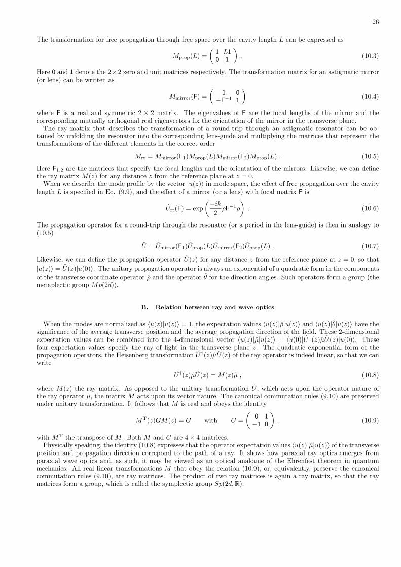
26

The transformation for free propagation through free space over the cavity length L can be expressed as

Mprop(L) =(

1 L10 1

). (10.3)

Here 0 and 1 denote the 2×2 zero and unit matrices respectively. The transformation matrix for an astigmatic mirror(or lens) can be written as

Mmirror(F) =(

1 0−F−1 1

)(10.4)

where F is a real and symmetric 2 × 2 matrix. The eigenvalues of F are the focal lengths of the mirror and thecorresponding mutually orthogonal real eigenvectors fix the orientation of the mirror in the transverse plane.

The ray matrix that describes the transformation of a round-trip through an astigmatic resonator can be ob-tained by unfolding the resonator into the corresponding lens-guide and multiplying the matrices that represent thetransformations of the different elements in the correct order

Mrt = Mmirror(F1)Mprop(L)Mmirror(F2)Mprop(L) . (10.5)

Here F1,2 are the matrices that specify the focal lengths and the orientation of the mirrors. Likewise, we can definethe ray matrix M(z) for any distance z from the reference plane at z = 0.

When we describe the mode profile by the vector |u(z)〉 in mode space, the effect of free propagation over the cavitylength L is specified in Eq. (9.9), and the effect of a mirror (or a lens) with focal matrix F is

Urt(F) = exp(−ik

2ρF−1ρ

). (10.6)

The propagation operator for a round-trip through the resonator (or a period in the lens-guide) is then in analogy to(10.5)

U = Umirror(F1)Uprop(L)Umirror(F2)Uprop(L) . (10.7)

Likewise, we can define the propagation operator U(z) for any distance z from the reference plane at z = 0, so that|u(z)〉 = U(z)|u(0)〉. The unitary propagation operator is always an exponential of a quadratic form in the componentsof the transverse coordinate operator ρ and the operator θ for the direction angles. Such operators form a group (themetaplectic group Mp(2d)).

B. Relation between ray and wave optics

When the modes are normalized as 〈u(z)|u(z)〉 = 1, the expectation values 〈u(z)|ρ|u(z)〉 and 〈u(z)|θ|u(z)〉 have thesignificance of the average transverse position and the average propagation direction of the field. These 2-dimensionalexpectation values can be combined into the 4-dimensional vector 〈u(z)|µ|u(z)〉 = 〈u(0)|U†(z)µU(z)|u(0)〉. Thesefour expectation values specify the ray of light in the transverse plane z. The quadratic exponential form of thepropagation operators, the Heisenberg transformation U†(z)µU(z) of the ray operator is indeed linear, so that we canwrite

U†(z)µU(z) = M(z)µ , (10.8)

where M(z) the ray matrix. As opposed to the unitary transformation U , which acts upon the operator nature ofthe ray operator µ, the matrix M acts upon its vector nature. The canonical commutation rules (9.10) are preservedunder unitary transformation. It follows that M is real and obeys the identity

MT(z)GM(z) = G with G =(

0 1−1 0

), (10.9)

with MT the transpose of M . Both M and G are 4× 4 matrices.Physically speaking, the identity (10.8) expresses that the operator expectation values 〈u(z)|µ|u(z)〉 of the transverse

position and propagation direction correpond to the path of a ray. It shows how paraxial ray optics emerges fromparaxial wave optics and, as such, it may be viewed as an optical analogue of the Ehrenfest theorem in quantummechanics. All real linear transformations M that obey the relation (10.9), or, equivalently, preserve the canonicalcommutation rules (9.10), are ray matrices. The product of two ray matrices is again a ray matrix, so that the raymatrices form a group, which is called the symplectic group Sp(2d,R).

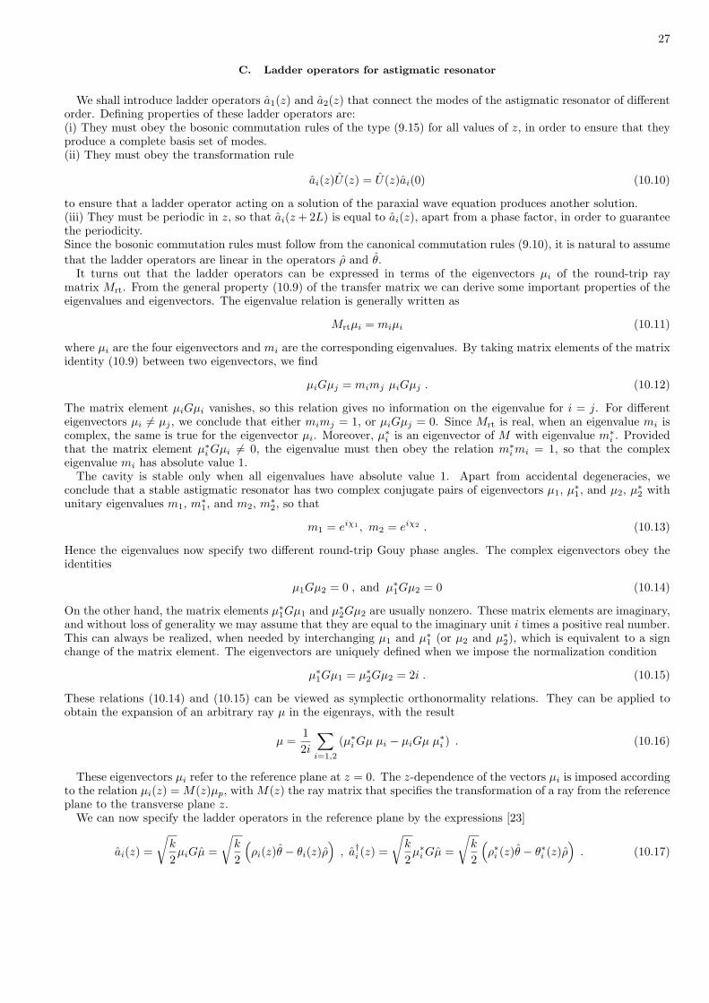
27

C. Ladder operators for astigmatic resonator

We shall introduce ladder operators a1(z) and a2(z) that connect the modes of the astigmatic resonator of differentorder. Defining properties of these ladder operators are:(i) They must obey the bosonic commutation rules of the type (9.15) for all values of z, in order to ensure that theyproduce a complete basis set of modes.(ii) They must obey the transformation rule

ai(z)U(z) = U(z)ai(0) (10.10)

to ensure that a ladder operator acting on a solution of the paraxial wave equation produces another solution.(iii) They must be periodic in z, so that ai(z + 2L) is equal to ai(z), apart from a phase factor, in order to guaranteethe periodicity.Since the bosonic commutation rules must follow from the canonical commutation rules (9.10), it is natural to assumethat the ladder operators are linear in the operators ρ and θ.

It turns out that the ladder operators can be expressed in terms of the eigenvectors µi of the round-trip raymatrix Mrt. From the general property (10.9) of the transfer matrix we can derive some important properties of theeigenvalues and eigenvectors. The eigenvalue relation is generally written as

Mrtµi = miµi (10.11)

where µi are the four eigenvectors and mi are the corresponding eigenvalues. By taking matrix elements of the matrixidentity (10.9) between two eigenvectors, we find

µiGµj = mimj µiGµj . (10.12)

The matrix element µiGµi vanishes, so this relation gives no information on the eigenvalue for i = j. For differenteigenvectors µi 6= µj , we conclude that either mimj = 1, or µiGµj = 0. Since Mrt is real, when an eigenvalue mi iscomplex, the same is true for the eigenvector µi. Moreover, µ∗i is an eigenvector of M with eigenvalue m∗

i . Providedthat the matrix element µ∗i Gµi 6= 0, the eigenvalue must then obey the relation m∗

i mi = 1, so that the complexeigenvalue mi has absolute value 1.

The cavity is stable only when all eigenvalues have absolute value 1. Apart from accidental degeneracies, weconclude that a stable astigmatic resonator has two complex conjugate pairs of eigenvectors µ1, µ∗1, and µ2, µ∗2 withunitary eigenvalues m1, m∗

1, and m2, m∗2, so that

m1 = eiχ1 , m2 = eiχ2 . (10.13)

Hence the eigenvalues now specify two different round-trip Gouy phase angles. The complex eigenvectors obey theidentities

µ1Gµ2 = 0 , and µ∗1Gµ2 = 0 (10.14)

On the other hand, the matrix elements µ∗1Gµ1 and µ∗2Gµ2 are usually nonzero. These matrix elements are imaginary,and without loss of generality we may assume that they are equal to the imaginary unit i times a positive real number.This can always be realized, when needed by interchanging µ1 and µ∗1 (or µ2 and µ∗2), which is equivalent to a signchange of the matrix element. The eigenvectors are uniquely defined when we impose the normalization condition

µ∗1Gµ1 = µ∗2Gµ2 = 2i . (10.15)

These relations (10.14) and (10.15) can be viewed as symplectic orthonormality relations. They can be applied toobtain the expansion of an arbitrary ray µ in the eigenrays, with the result

µ =12i

∑

i=1,2

(µ∗i Gµ µi − µiGµ µ∗i ) . (10.16)

These eigenvectors µi refer to the reference plane at z = 0. The z-dependence of the vectors µi is imposed accordingto the relation µi(z) = M(z)µp, with M(z) the ray matrix that specifies the transformation of a ray from the referenceplane to the transverse plane z.

We can now specify the ladder operators in the reference plane by the expressions [23]

ai(z) =

√k

2µiGµ =

√k

2

(ρi(z)θ − θi(z)ρ

), a†i (z) =

√k

2µ∗i Gµ =

√k

2

(ρ∗i (z)θ − θ∗i (z)ρ

). (10.17)

28

where we separate the vectors µi(z) in the two-dimensional subvectors ρi(z) and θi(z). The bosonic commutationrules are ensured by the relations (10.14) and (10.15). The z-dependence of these ladder operators indeed obeys therelation (10.10), as can be checked by using the Ehrenfest transformation (10.8). Finally, the ladder operators havethe same periodicity as the eigenrays, so that ai(z + 2L) = exp(iχi)a(z).

The expressions for the ladder operators in terms of the ray operator µ can be directly inverted by using the generalexpansion (10.16). When we substitute the operator µ for µ, we obtain

µ =1

i√

2k

∑

i=1,2

(µia

†i − µ∗i ai

). (10.18)

This expression is valid for all transverse planes z.

D. Structure of the modes and resonance spectrum

The full set of modes for all values of z is now determined by the relations

|unm(z)〉 =1√

n!m!

(a†1(z)

)n (a†2(z)

)m

|u00(z)〉 , (10.19)

in terms of the fundamental mode |u00(z)〉. An explicit analytical expression for the normalized fundamental modecan be given when we introduce the 2× 2 matrices

R(z) = (ρ1(z) ρ2(z)) and T(z) = (θ1(z) θ2(z)) , (10.20)

in terms of the two-dimensional column vectors ρi and θi. The symplectic orthonormality properties (10.14) and(10.15) of the vectors µ1,2 can be expressed as

R†T− T†R = 2i1 , and RTT− TTR = 0 (10.21)

which hold for all values of z. An explicit analytical expression of the normalized mode function as it propagatesthrough the lens guide is given by

u00(ρ, z) =

√k

π detR(z)exp (−kρS(z)ρ/2) , (10.22)

where S = −iTR−1 is a 2 × 2 matrix. Because of the definitions of R and T in terms of the eigenvectors of theround-trip matrix M , the fundamental mode returns to itself after a round trip, as expressed by

|u00(z + 2L)〉 = |u00(z)〉 exp(−i(χ1 + χ2)/2) . (10.23)

It is directly checked that acting upon |u00〉 with the lowering operators a1(z) and a2(z) gives zero, and that it obeysthe paraxial wave equation both in the sections of free propagation [24], and across the lenses [23]. Moreover, thesecond relation (10.21) guarantees that S is symmetric. This is obvious when we multiply the relation from the leftwith (RT)−1, and from the right with R−1.

The real and imaginary parts Sr and Si of S respectively characterize the astigmatism of the intensity and phasepatterns. The real part can be written as Sr = (−iTR−1 + i(R†)−1T†)/2. With the first relation (10.21) this showsthat RSrR

† = 1. This leads to the identity

RR† = S−1r (10.24)

This shows that Sr is positive definite, so that the fundamental mode is square-integrable. The curves of constantintensity are ellipses. Depending on the sign of det Si the curves of constant phase are ellipses, hyperbolas or parallelstraight lines. Under free propagation, S is a slowly varying smooth function of z. Optical elements, on the otherhand, may instantaneously modify the astigmatism. The astigmatism of both the intensity and the phase patterns ischaracterized by two widths in mutually perpendicular directions and one angle that specifies the orientation of thecurves of constant intensity or phase. As opposed to R and T, the matrix S is a matrix in real space ρ = (x, y) andtransforms accordingly under coordinate transformations.

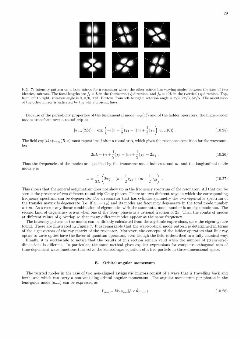
29

FIG. 7: Intensity pattern on a fixed mirror for a resonator where the other mirror has varying angles between the axes of twoidentical mirrors. The focal lengths are fξ = L in the (horizontal) ξ-direction, and fη = 10L in the (vertical) η-direction. Top,from left to right: rotation angle is 0, π/6, π/3. Bottom, from left to right: rotation angle is π/2, 2π/3, 5π/6. The orientationof the other mirror is indicated by the white crossing lines.

Because of the periodicity properties of the fundamental mode |u00(z)〉 and of the ladder operators, the higher-ordermodes transform over a round trip as

|unm(2L)〉 = exp(−i(n +

12)χ1 − i(m +

12)χ2

)|unm(0)〉 . (10.25)

The field exp(ikz)unm(R, z) must repeat itself after a round trip, which gives the resonance condition for the wavenum-ber

2kL− (n +12)χ1 − (m +

12)χ2 = 2πq . (10.26)

Thus the frequencies of the modes are specified by the transverse mode indices n and m, and the longitudinal modeindex q is

ω =c

2L

(2πq + (n +

12)χ1 + (m +

12)χ2

). (10.27)

This shows that the general astigmatism does not show up in the frequency spectrum of the resonator. All that can beseen is the presence of two different round-trip Gouy phases. There are two different ways in which the correspondingfrequency spectrum can be degenerate. For a resonator that has cylinder symmetry the two eigenvalue spectrum ofthe transfer matrix is degenerate (i.e. if χ1 = χ2) and its modes are frequency degenerate in the total mode numbern+m. As a result any linear combination of eigenmodes with the same total mode number is an eigenmode too. Thesecond kind of degeneracy arises when one of the Gouy phases is a rational fraction of 2π. Then the combs of modesat different values of q overlap so that many different modes appear at the same frequency.

The intensity pattern of the modes can be directly calculated from the algebraic expressions, once the eigenrays arefound. These are illustrated in Figure 7. It is remarkable that the wave-optical mode pattern is determined in termsof the eigenvectors of the ray matrix of the resonator. Moreover, the concepts of the ladder operators that link rayoptics to wave optics have the flavor of quantum operators, even though the field is described in a fully classical way.

Finally, it is worthwhile to notice that the results of this section remain valid when the number of (transverse)dimensions is different. In particular, the same method gives explicit expressions for complete orthogonal sets oftime-dependent wave functions that solve the Schrodinger equation of a free particle in three-dimensional space.

E. Orbital angular momentum

The twisted modes in the case of two non-aligned astigmatic mirrors consist of a wave that is travelling back andforth, and which can carry a non-vanishing orbital angular momentum. The angular momentum per photon in thelens-guide mode |unm〉 can be expressed as

Lnm = ~k〈unm|ρ× θ|unm〉 (10.28)

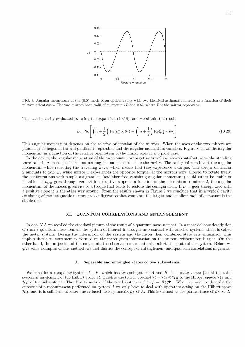
30

FIG. 8: Angular momentum in the (0,0) mode of an optical cavity with two identical astigmatic mirrors as a function of theirrelative orientation. The two mirrors have radii of curvature 2L and 20L, where L is the mirror separation.

This can be easily evaluated by using the expansion (10.18), and we obtain the result

Lnm~k

[ (n +

12

)Re(ρ∗1 × θ1) +

(m +

12

)Re(ρ∗2 × θ2)

](10.29)

This angular momentum depends on the relative orientation of the mirrors. When the axes of the two mirrors areparallel or orthogonal, the astigmatism is separable, and the angular momentum vanishes. Figure 8 shows the angularmomentum as a function of the relative orientation of the mirror axes in a typical case.

In the cavity, the angular momentum of the two counter-propagating travelling waves contributing to the standingwave cancel. As a result their is no net angular momentum inside the cavity. The cavity mirrors invert the angularmomentum while reflecting the travelling wave, which means that they experience a torque. The torque on mirror2 amounts to 2cLnm, while mirror 1 experiences the opposite torque. If the mirrors were allowed to rotate freely,the configurations with simple astigmatism (and therefore vanishing angular momentum) could either be stable orinstable. If Lnm goes through zero with a negative slope as a function of the orientation of mirror 2, the angularmomentum of the modes gives rise to a torque that tends to restore the configuration. If Lnm goes though zero witha positive slope it is the other way around. From the results shown in Figure 8 we conclude that in a typical cavityconsisting of two astigmatic mirrors the configuration that combines the largest and smallest radii of curvature is thestable one.

XI. QUANTUM CORRELATIONS AND ENTANGLEMENT

In Sec. VA we recalled the standard picture of the result of a quantum measurement. In a more delicate descriptionof such a quantum measurement the system of interest is brought into contact with another system, which is calledthe meter system. During the interaction of the system and the meter their combined state gets entangled. Thisimplies that a measurement performed on the meter gives information on the system, without touching it. On theother hand, the projection of the meter into the observed meter state also affects the state of the system. Before wegive some examples of this method, we first discuss the concept of entanglement and quantum correlations in general.

A. Separable and entangled states of two subsystems

We consider a composite system A ∪ B, which has two subsystems A and B. The state vector |Ψ〉 of the totalsystem is an element of the Hilbert space H, which is the tensor product H = HA⊗HB of the Hilbert spaces HA andHB of the subsystems. The density matrix of the total system is then ρ = |Ψ〉〈Ψ|. When we want to describe theoutcome of a measurement performed on system A we only have to deal with operators acting on the Hilbert spaceHA, and it is sufficient to know the reduced density matrix ρA of A. This is defined as the partial trace of ρ over B.

31

After choosing a basis set of orthonormal states |φBj〉 of the subsystem B, the reduced density matrix of A is definedas

ρA = TrB ρ =∑

j

〈φBj |Ψ〉〈Ψ|φBj〉 . (11.1)

Note that the inner product 〈φBj |Ψ〉 is still a vector in HA, so that Eq. (11.1) indeed defines a density matrix forsubsystem A. For instance, an observable QA of system A does not act on HB , so that we can write its expectationvalue as

〈QA〉 =∑

j

〈Ψ|φBj〉QA〈φBj |Ψ〉 = TrA ρAQA . (11.2)

The reduced density matrix ρB of the subsystem B is defined in an analogous way as

ρB = TrA ρ =∑

i

〈φAi|Ψ〉〈Ψ|φAi〉 . (11.3)

Just as all density matrices, the reduced density matrices ρA and ρB are Hermitian, normalized and positive definite.A state vector |Ψ〉 that factorizes as the tensor product |ψA〉⊗ |ψB〉 of a state vector |ψA〉 in HA and a state vector

|ψB〉 in HB is called as separable state. For such a state, the reduced density matrices of subsystems A and B aregiven by ρA = |ψA〉〈ψA| and ρB = |ψB〉〈ψB |, which are both pure states. Such a state vector is called separable.The opposite is also true: when the state vector |Ψ〉 produces reduced density matrices ρA and ρB that are bothpure states, then the state vector |Ψ〉 is separable. A non-separable state vector |Ψ〉 is called an entangled state. Itproduces reduced density matrices ρA and ρB that describe mixed states of subsystem A and B. In an entangledstate it is not possible to attach a state vector to the system A or to the system B. The importance of the concept ofentanglement arises from the fact that a measurement on the subsystem A will affect not only the state of A, but alsothat of B. In order to clarify this, we first demonstrate that a state vector of two systems can always be expanded asa single summation over a double orthonormal basis.

A subsystem contains a fraction of the degrees of freedom of the system. Therefore, a system can usually be dividedin subsystems in several ways. It is important to notice that the concept of entanglement refers to one such division.The concept of entanglement is particularly useful when the two subsystems are spatially separated.

B. Schmidt decomposition and entanglement

Two given orthonormal basis sets |φAi〉 and |φBj〉 of the two subspaces HA and HB define a basis set of productvectors |φAi〉⊗|φBj〉 of the combined space H. Therefore an arbitrary state vector |Ψ〉 in H can always be expandedas a double expansion

|Ψ〉 =∑

i

∑

j

cij |φAi〉 ⊗ |φBj〉 . (11.4)

It is not immediately clear from the set of coefficients cij whether or not the state |Ψ〉 is separable.We want to show that an arbitrary pure state |Ψ〉 in H can be written as a single summation over product states.

The basis sets |ψAn〉 and |ψBn〉 must be properly selected, and depend on the state |Ψ〉. We first consider thereduced density matrix ρA of A. Since ρA is Hermitian, positive definite and normalized, it has a complete set ofeigenvectors, which we call |ψAn〉. The corresponding eigenvalues sn are real and non-negative, and because of thenormalization they add up to 1. Since the set |ψAn〉 is orthonormal and complete, we can expand the state |Ψ〉 asthe single sum

|Ψ〉 =∑

n

|ψAn〉 ⊗ 〈ψAn|Ψ〉 . (11.5)

Notice that the inner products 〈ψAn|Ψ〉 are state vectors in HB . The inner products of two of these vectors can berewritten as

〈Ψ|ψAn〉〈ψAm|Ψ〉 = TrB〈ψAm|Ψ〉〈Ψ|ψAn〉 = 〈ψAm|ρA|ψAn〉 = snδmn , (11.6)

which shows that they are orthogonal. The eigenstates |ψAn〉 of ρA with eigenvalue zero have no overlap with |Ψ〉,and can be omitted in the expansion (11.5). For nonzero eigenvalues sn we define the orthonormal states

|φBn〉 = 〈ψAn|Ψ〉/√sn (11.7)

32

of B. Equation (11.5) can therefore be replaced by

|Ψ〉 =∑

n

√sn |ψAn〉 ⊗ |ψBn〉 . (11.8)

Thus we have proven that an arbitrary state vector |Ψ〉 of A∪B can be written as a single summation over productstates |ψAn〉 ⊗ |ψBn〉, where the sets |ψAn〉 and |ψBn〉 are both orthonormal. This expansion (11.8) is calledSchmidt’s decomposition, and the two basis sets are called the Schmidt bases. It will be clear that these basis setsdepend on the state |Ψ〉. On these bases the two reduced density matrices ρA and ρB have the same diagonal form,with the eigenvalues sn as diagonal elements. These eigenvalues sn represent the populations of the states |ψAn〉 and|ψBn〉. The number of summands in the expansion (11.8) is maximally equal to N , defined as the minimum of thenumber of dimensions of the state spaces HA and HB of A and B. The state |Ψ〉 is separable only if the expansion(11.8) contains just a single term. When the reduced density matrices ρA and ρB represent mixed states, the state|Ψ〉 is entangled. The entanglement is maximal when the populations sn are all equal. Then they must be given by1/N , and the mixture in each one of the reduced density matrices is maximal.

C. Effect of measurement on an entangled state

When the system A ∪ B is in the state |Ψ〉, and the observable QA of the subsystem A is measured, the result isthe eigenvalue qA with the probability

pA = 〈Ψ|PA|Ψ〉 = TrρPA = TrAρAPA , (11.9)

where PA = |ψA〉〈ψA| is the projection operator on the corresponding eigenstate |ψA〉. This notation is analogouswith Eqs. (5.3) and (5.7). Just as indicated in Eq. (5.4), directly after the measurement the normalized state vectoris given by the expression

|Ψafter〉 = PA|Ψ〉/√pA . (11.10)

The reduced density matrix of subsystem A after the measurement is

ρA,after = TrB |Ψafter〉〈Ψafter| = PAρAPA/pA , (11.11)

which is similar to Eq. (5.8). This reduced density matrix of A corresponds to the pure state |ψA〉. Therefore thestate after the measurement is separable in the form

|Ψafter〉 = |ψA〉 ⊗ |ψB〉 . (11.12)

When the state |Ψ〉 is written as a Schmidt expansion (11.8), the state |ψB〉 takes the form

|ψB〉 =∑

n

√sn

pA〈ψA|ψAn〉|ψBn〉 , (11.13)

where

pA =∑

n

sn|〈ψA|ψAn〉|2 (11.14)

is the probability for detection of the state |ψA〉.

D. Quantum non-locality

We find that the subsystem B after the measurement is in the pure state (11.13). This state obviously depends onthe outcome of the measurement performed on A. For instance, |ψB〉 coincides with the Schmidt state |ψBn〉 when|ψA〉 = |φAn〉, so that the system B can be put in any of its Schmidt basis vectors for a well-selected measurementon A. However, this conclusion is not particularly quantum-mechanical. It could simply reflect a classical correlationbetween the states of system A and system B: there is a probability sn that system A is in the state |ψAn〉 andsystem B in the state |ψBn〉. However, Eq. (11.13) shows that the subsystem B can also get projected into a state

33

that is any linear combination of the Schmidt states |ψBn〉. The Schmidt states |ψBn〉 are orthogonal, and can beregarded as different eigenstates of a single observable. In this sense, these states are mutually compatible. But linearcombinations of the Schmidt states correspond to incompatible observables. It turns out that the subsystem B canend up in an eigenstate of different non-commuting operators. Moreover, the final state of B depends on actions andobservations on the subsystem A.

This is surprising when we realize that the subsystems A and B could well be physically separated by an arbitrarydistance. When the combined system is prepared in an entangled state, the subsystems A and B can be displaced,without changing the entanglement of their internal states. When a measurement is performed on system A, it is hardto imagine that the state of the remote subsystem B can be affected by that. After all, the subsystem B is not touchedby the measurement apparatus. Nevertheless, these results show that the state vector of one subsystem (B) can beaffected by actions performed on another system (A), that may be arbitrarily far away. It can just as well be in aneigenstate of one observable QB , or in an eigenstate of another, non-compatible observable Q′B , that does not commutewith QB . On the other hand, since the measurement results (the corresponding eigenvalues of these operators) can bepredicted with certainty, a logical conclusion would be that the observables factually have these values, even before(or without) the actual measurement on A. In the language of the famous paper by Einstein, Podolsky and Rosen[25] (EPR), these values are elements of physical reality. Since quantum mechanics does not predict these eigenvaluesof non-commuting operators, the authors conclude that there are elements of reality that quantum mechanics doesnot describe. This leads them to the logical conclusion that quantum mechanics is incomplete.

In the original paper of EPR a state of two particles was considered, with the two-particle wave function (in onedimension)

Ψ(x1, x2) = δ(x1 − x2 − L) =1

2π~

∫ ∞

−∞dp exp

(i

~p(x1 − x2 − L)

). (11.15)

Since the integrand factorizes into separate contributions for each particle, this expression can be viewed as a con-tinuous version of the Schmidt decomposition (11.8), with p replacing the index i. This state is an eigenstate of therelative position x1 − x2, with eigenvalue L, and of the total momentum −i~ ((∂/∂x1) + (∂/∂x2)), with eigenvaluezero. Hence, if the position of particle 1 is measured with the outcome x0, the position of particle 2 is x0 − L. Ifthe momentum of particle 1 is measured with the outcome p0, then the momentum of particle 2 is −p0. Since theseeigenvalues of observables of particle 2 can get a well-determined value without perturbing the state of particle 2, theyare elements of reality in the sense of EPR [25]. This means that these incompatible eigenvalues must both be reallythere, as properties of the state of particle 2, even though quantum mechanics does not allow to assign simultaneouslythe two different eigenstates of position and momentum to the system. EPR concluded that reality has propertiesthat quantum mechanics does not describe. In this sense, quantum mechanics is incomplete. Bell has formulated hisfamous inequalities for the correlations between measurement results of two subsystems, based on the assumptions ofreality (the result of a measurement is an element of reality) and locality (a measurement on A cannot affect the stateof B). Bell’s inequalities were originally derived for two entangled systems, each with a two-dimensional state space.In the language of the field of quantum information, a quantum system with two states is a quantum bit, or qubit.The prediction of quantum mechanics that Bell’s inequalities can be violated has been experimentally confirmed. Theconclusion is that realism and locality cannot both be correct. Nowadays, most physicists accept the conclusion thatthe reality argument must be abandoned. The alternative would be to accept an instantaneous change of the physicalsituation at the position of B, by actions that take place exclusively at the position of B.

We have shown that quantum mechanics allows to prepare a subsystem (B) in different pure states that are non-orthogonal, by actions that are performed exclusively on another subsystem (A). This feature of quantum mechanicsis called quantum non-locality. Its effects are clear and unambiguous, even though there is still a lot of debate on itsinterpretation. We stress that non-orthogonal states are eigenstates of non-commuting operators. This means thatthey are incompatible, since quantum mechanics does not allow the corresponding two observables to have preciselydetermined values.

This non-local effect on the state vector of a subsystem cannot be used to transfer information instantaneously fromthe location of A to the location of B. It is true that knowledge of the pure state (11.13) allows one to predict withcertainty the outcome of an appropriate measurement on B. However, this certainty is available only to someone whoknows what has been measured on A. Recall that the state vector cannot be determined by a single measurement,only by repeated measurements on an ensemble of systems prepared in the same state. Measurements performedon B, unconditioned by the settings of the measurement apparatus and the measurement outcomes on A, are fullydescribed by the reduced density matrix ρB alone.

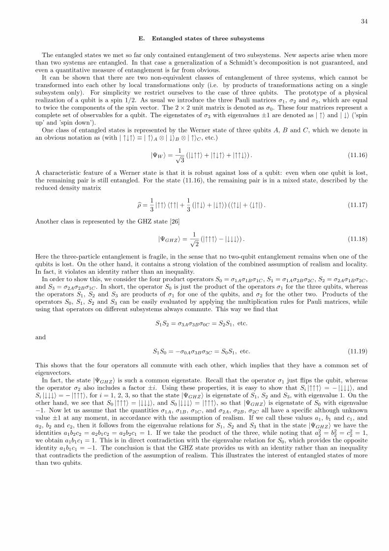
34

E. Entangled states of three subsystems

The entangled states we met so far only contained entanglement of two subsystems. New aspects arise when morethan two systems are entangled. In that case a generalization of a Schmidt’s decomposition is not guaranteed, andeven a quantitative measure of entanglement is far from obvious.

It can be shown that there are two non-equivalent classes of entanglement of three systems, which cannot betransformed into each other by local transformations only (i.e. by products of transformations acting on a singlesubsystem only). For simplicity we restrict ourselves to the case of three qubits. The prototype of a physicalrealization of a qubit is a spin 1/2. As usual we introduce the three Pauli matrices σ1, σ2 and σ3, which are equalto twice the components of the spin vector. The 2× 2 unit matrix is denoted as σ0. These four matrices represent acomplete set of observables for a qubit. The eigenstates of σ3 with eigenvalues ±1 are denoted as | ↑〉 and | ↓〉 (’spinup’ and ’spin down’).

One class of entangled states is represented by the Werner state of three qubits A, B and C, which we denote inan obvious notation as (with | ↑↓↑〉 ≡ | ↑〉A ⊗ | ↓〉B ⊗ | ↑〉C , etc.)

|ΨW 〉 =1√3

(|↓↑↑〉+ |↑↓↑〉+ |↑↑↓〉) . (11.16)

A characteristic feature of a Werner state is that it is robust against loss of a qubit: even when one qubit is lost,the remaining pair is still entangled. For the state (11.16), the remaining pair is in a mixed state, described by thereduced density matrix

ρ =13|↑↑〉 〈↑↑|+ 1

3(|↑↓〉+ |↓↑〉) (〈↑↓|+ 〈↓↑|) . (11.17)

Another class is represented by the GHZ state [26]

|ΨGHZ〉 =1√2

(|↑↑↑〉 − |↓↓↓〉) . (11.18)

Here the three-particle entanglement is fragile, in the sense that no two-qubit entanglement remains when one of thequbits is lost. On the other hand, it contains a strong violation of the combined assumption of realism and locality.In fact, it violates an identity rather than an inequality.

In order to show this, we consider the four product operators S0 = σ1Aσ1Bσ1C , S1 = σ1Aσ2Bσ2C , S2 = σ2Aσ1Bσ2C ,and S3 = σ2Aσ2Bσ1C . In short, the operator S0 is just the product of the operators σ1 for the three qubits, whereasthe operators S1, S2 and S3 are products of σ1 for one of the qubits, and σ2 for the other two. Products of theoperators S0, S1, S2 and S3 can be easily evaluated by applying the multiplication rules for Pauli matrices, whileusing that operators on different subsystems always commute. This way we find that

S1S2 = σ3Aσ3Bσ0C = S2S1, etc.

and

S1S0 = −σ0Aσ3Bσ3C = S0S1, etc. (11.19)

This shows that the four operators all commute with each other, which implies that they have a common set ofeigenvectors.

In fact, the state |ΨGHZ〉 is such a common eigenstate. Recall that the operator σ1 just flips the qubit, whereasthe operator σ2 also includes a factor ±i. Using these properties, it is easy to show that Si |↑↑↑〉 = − |↓↓↓〉, andSi |↓↓↓〉 = − |↑↑↑〉, for i = 1, 2, 3, so that the state |ΨGHZ〉 is eigenstate of S1, S2 and S3, with eigenvalue 1. On theother hand, we see that S0 |↑↑↑〉 = |↓↓↓〉, and S0 |↓↓↓〉 = |↑↑↑〉, so that |ΨGHZ〉 is eigenstate of S0 with eigenvalue−1. Now let us assume that the quantities σ1A, σ1B , σ1C , and σ2A, σ2B , σ2C all have a specific although unknownvalue ±1 at any moment, in accordance with the assumption of realism. If we call these values a1, b1 and c1, anda2, b2 and c2, then it follows from the eigenvalue relations for S1, S2 and S3 that in the state |ΨGHZ〉 we have theidentities a1b2c2 = a2b1c2 = a2b2c1 = 1. If we take the product of the three, while noting that a2

2 = b22 = c2

2 = 1,we obtain a1b1c1 = 1. This is in direct contradiction with the eigenvalue relation for S0, which provides the oppositeidentity a1b1c1 = −1. The conclusion is that the GHZ state provides us with an identity rather than an inequalitythat contradicts the prediction of the assumption of realism. This illustrates the interest of entangled states of morethan two qubits.

35

XII. CREATION AND APPLICATION OF ENTANGLEMENT

A. Atom and a cavity mode

The simplest way of creating entangled states of two systems is to make them interact. When the combined systemA ∪ B is initially in a separable state |Ψin〉 = |ψ0A〉 ⊗ |ψ0B〉, the final state |Ψout〉 = U(|ψ0A〉 ⊗ |ψ0B〉) after theinteraction can easily be entangled. Here the unitary operator U describes the evolution of the combined systemduring some interaction time. When the system A is then detected to be in the state |ψ1A〉, the state of subsystemB can be given by

|ψ1B〉 = 〈ψ1A|U |ψ0A〉|ψ0B〉/√p1A . (12.1)

The term 〈ψ1A|U |ψ0A〉 is an operator acting on HB . This operator is not unitary in general. The probability p1A forthe detection of state |ψ1A〉 is |〈ψ1A|Ψout〉|2.

A practical and flexible example of two interacting systems is a two-state atom interacting with a mode of theradiation field in a cavity. The atom has a lower state |g〉 and a higher state |e〉. The mode of the radiation fieldhas the photon number states |n〉 as basis. In the nearly resonant case, when the frequency separation ω0 betweenthe atomic states is close to the mode frequency ω, the rotating-wave approximation is valid, and the combined state|g, n〉 is only coupled to the state |e, n− 1〉. The coupling term of the Hamiltonian is

〈e, n− 1|H|g, n〉 = −12~Ωn , (12.2)

with the Rabi frequency Ωn =√

nΩ1 proportional to the square root of the photon number.We consider two limiting cases. In the resonant case, the frequencies of the atom and the mode are identical. For

the initial state |Ψ(0)〉 = |g, n〉, the time-dependent state takes the form

|Ψ(t)〉 = cos(12Ωnt)|g, n〉+ i sin(

12Ωnt)|e, n− 1〉 . (12.3)

When the two states are viewed as the eigenstates of a spin 1/2, this evolution is equivalent to a rotation withfrequency Ωn about the x-axis of a spin that starts in the negative z-direction. An atom that traverses the cavitywill interact with the mode during a finite time T , and after the passage the atom and the mode will be entangled ingeneral. For instance, when ΩnT = π/2 (a π/2-pulse), the final state will be |Ψ(T )〉 = (|g, n〉+ i|e, n− 1〉)/√2.

When the frequency difference ∆ = ω−ω0 is large compared to Ωn, the initial state |g, n〉 is followed adiabatically,and the atom-mode coupling introduces an energy shift ~Ω2

n/(4∆) during the interaction time. After an interactiontime T , this gives an additional phase shift φn, with φ = Ω2

1T/(4∆). The phase shift is proportional to the photonnumber.

For Rydberg atoms in a high-quality microwave cavity, the parameters can be chosen such that in the resonantcase even the one-photon Rabi frequency Ω1 is large enough to allow a sizable state change during the passage timeT . Also the phase change per photon in the off-resonance case can be significant. Over the years, such systems havebeen developed and extensively used by several groups, notably at the Ecole Normale Superieure in Paris and theMax-Planck-Institut fur Quantenoptik in Garching.

B. Non-destructive photon measurement

In many cases it is advantageous to perform a measurement indirectly, without touching the system of interest.This is the case for the detection of photons, defined as the quanta of a mode of the radiation field. When a photonis detected by a photomultiplier, the photon is absorbed, and it does not survive the detection process. This canbe avoided by creating a correlation between the system of interest (in this case the mode), and some other system,which is called the meter. We discuss a few simple cases, that have been actually applied in the literature, where anatom plays the part of the meter.

We consider the atom-cavity system in the resonant case. The lower state |g〉 is coupled by the cavity photons tothe state |e〉. In addition, the state |g〉 is also coupled to a third state |i〉 by a classical field, either in the preparationstage (prior to the passage through the cavity) or in the detection stage (after the passage). Suppose that the settingis such that the initial state |g, 1〉 undergoes a 2π pulse, so that Ω1T = 2π. Then the state evolves into the state−|g, 1〉 after passing the cavity. Since the state |i〉 is not coupled to the mode, it remains unchanged, which impliesthat the superposition state (|i〉 + |g〉)/√2 passing mode is changed into the state (|i〉 − |g〉)/√2 when there is one

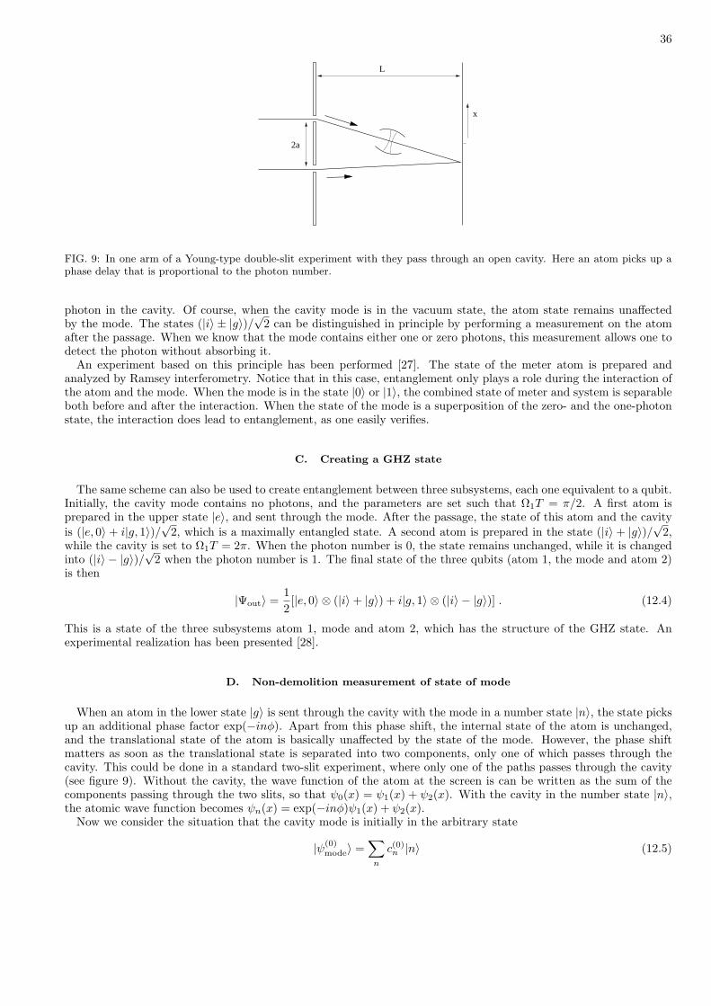
36

L

x

2a

FIG. 9: In one arm of a Young-type double-slit experiment with they pass through an open cavity. Here an atom picks up aphase delay that is proportional to the photon number.

photon in the cavity. Of course, when the cavity mode is in the vacuum state, the atom state remains unaffectedby the mode. The states (|i〉 ± |g〉)/√2 can be distinguished in principle by performing a measurement on the atomafter the passage. When we know that the mode contains either one or zero photons, this measurement allows one todetect the photon without absorbing it.

An experiment based on this principle has been performed [27]. The state of the meter atom is prepared andanalyzed by Ramsey interferometry. Notice that in this case, entanglement only plays a role during the interaction ofthe atom and the mode. When the mode is in the state |0〉 or |1〉, the combined state of meter and system is separableboth before and after the interaction. When the state of the mode is a superposition of the zero- and the one-photonstate, the interaction does lead to entanglement, as one easily verifies.

C. Creating a GHZ state

The same scheme can also be used to create entanglement between three subsystems, each one equivalent to a qubit.Initially, the cavity mode contains no photons, and the parameters are set such that Ω1T = π/2. A first atom isprepared in the upper state |e〉, and sent through the mode. After the passage, the state of this atom and the cavityis (|e, 0〉 + i|g, 1〉)/√2, which is a maximally entangled state. A second atom is prepared in the state (|i〉 + |g〉)/√2,while the cavity is set to Ω1T = 2π. When the photon number is 0, the state remains unchanged, while it is changedinto (|i〉 − |g〉)/√2 when the photon number is 1. The final state of the three qubits (atom 1, the mode and atom 2)is then

|Ψout〉 =12[|e, 0〉 ⊗ (|i〉+ |g〉) + i|g, 1〉 ⊗ (|i〉 − |g〉)] . (12.4)

This is a state of the three subsystems atom 1, mode and atom 2, which has the structure of the GHZ state. Anexperimental realization has been presented [28].

D. Non-demolition measurement of state of mode

When an atom in the lower state |g〉 is sent through the cavity with the mode in a number state |n〉, the state picksup an additional phase factor exp(−inφ). Apart from this phase shift, the internal state of the atom is unchanged,and the translational state of the atom is basically unaffected by the state of the mode. However, the phase shiftmatters as soon as the translational state is separated into two components, only one of which passes through thecavity. This could be done in a standard two-slit experiment, where only one of the paths passes through the cavity(see figure 9). Without the cavity, the wave function of the atom at the screen is can be written as the sum of thecomponents passing through the two slits, so that ψ0(x) = ψ1(x) + ψ2(x). With the cavity in the number state |n〉,the atomic wave function becomes ψn(x) = exp(−inφ)ψ1(x) + ψ2(x).

Now we consider the situation that the cavity mode is initially in the arbitrary state

|ψ(0)mode〉 =

∑n

c(0)n |n〉 (12.5)

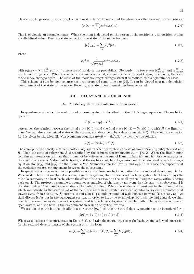
37

Then after the passage of the atom, the combined state of the mode and the atom takes the form in obvious notation

〈x|Ψ0〉 =∑

n

c(0)n ψn(x)|n〉 , (12.6)

This is obviously an entangled state. When the atom is detected on the screen at the position x1, its position attainsa well-defined value. Due this state reduction, the state of the mode becomes

|ψ(1)mode〉 =

∑n

c(1)n |n〉 , (12.7)

where

c(1)n =

1√p0(x0)

c(0)n ψn(x0) , (12.8)

with p0(x0) =∑

n |c(0)n ψn(x0)|2 a measure of the detection probability. Obviously, the two states |ψ(0)

mode〉 and |ψ(1)mode〉

are different in general. When the same procedure is repeated, and another atom is sent through the cavity, the stateof the mode changes again. The state of the mode no longer changes when it is reduced to a single number state.

This scheme of step-by-step collapse has been proposed some time ago [29]. It can be viewed as a non-demolitionmeasurement of the state of the mode. Recently, a related measurement has been reported.

XIII. DECAY AND DECOHERENCE

A. Master equation for evolution of open system

In quantum mechanics, the evolution of a closed system is described by the Schrodinger equation. The evolutionoperator

U(t) = exp(−iHt/~) (13.1)

determines the relation between the initial state |Ψ(0)〉 and the final state |Ψ(t)〉 = U(t)|Ψ(0)〉, with H the Hamilto-nian. We can also allow mixed states of the system, and describe it by a density matrix ρ(t). The evolution equationfor ρ is given by the Liouville-Von Neumann equation dρ/dt = −i[H, ρ]/~, which has the solution

ρ(t) = U(t)ρ(0)U†(t) . (13.2)

The concept of the density matrix is particularly useful when the system consists of two interacting subsystems A andB. Then the state of subsystem A is described by the reduced density matrix ρA = TrB ρ. When the Hamiltoniancontains an interaction term, so that it can not be written as the sum of Hamiltonians HA and HB for the subsystems,the evolution operator U does not factorize, and the evolution of the subsystems cannot be described by a Schrodingerequation (for |ψA〉 and |ψB〉) or the Liouville-Von Neumann equation (for ρA and ρB). In this case one expects thatthe evolution creates entanglement between the subsystems.

In special cases it turns out to be possible to obtain a closed evolution equation for the reduced density matrix ρA.We consider the situation that A is a small quantum system, that interacts with a large system B. Then B plays therole of a reservoir, or a heat bath, where the effect of the reservoir on the small system dissipates away, without actingback on A. The prototype example is spontaneous emission of photons by an atom. In this case, the subsystem A isthe atom, while B represents the modes of the radiation field. When the modes of interest are in the vacuum state,which we indicate as the state |ψB0〉 of the field, the atom in an excited state can spontaneously emit a photon, thattravels away from the atom. Spontaneous emission is a simple example of a dissipative irreversible process, and weshall discuss it further in the subsequent section. In order to keep the terminology both simple and general, we shallrefer to the small subsystem A as the system, and to the large subsystem B as the bath. The system A is then anopen system, and the bath is the environment in which the system evolves.

We assume that the bath is initially in a pure state |φB0〉, so that the initial density matrix has the factorized form

ρ(0) = ρA(0)⊗ (|φB0〉〈φB0|) . (13.3)

When we substitute this initial state in Eq. (13.2), and take the partial trace over the bath, we find a formal expressionfor the reduced density matrix of the system A in the form

ρA(t) =∑

ν

Eν(t)ρA(0)E†ν(t) =

∑ν

Eν ρA(0) , (13.4)

38

where the operators Eν are defined by

Eν(t) = 〈φBν |U(t)|φB0〉 . (13.5)

Since the operator U acts on the state space HA⊗HB of the combined system A∪B, the matrix elements 〈φBν |U |φB0〉are still operators on HA. The number of indices ν is equal to the number of dimensions dB of HB , which is verylarge compared to the number of dimensions dA of HA. Obviously, since the product Eν ρAE†

ν = Eν ρA is a linearmap acting on the density matrix ρA, and since ρA is determined by d2

A numbers, there can be no more than d2A

independent ones of these maps. In practice, we can always model the bath by a number of different maps Eν that isnot larger than d2

A.Equation (13.4) gives the density matrix ρA(t) after the evolution as a linear map of the initial density matrix

ρA(0). The representation (13.4) of the map is called an operator-sum representation. The map conserves the trace ofthe density matrix, which follows from the unitarity of the evolution operator U(t). Another way to formulate traceconservation is the normalization condition for the operators Eν

∑ν

E†νEν = IA , (13.6)

which follows from the completeness of the basis of states |φBν〉 of the bath.The states |φBν〉 form an orthonormal basis of the state space of the bath. Notice that at times t = 0, the

operators Eν vanish for ν 6= 0, whereas E0(0) = IA is the unit operator on HA. In order to derive a differentialequation for ρA, we consider small evolution times dt, and evaluate the change in ρA to first order. We write

ρA(dt) = ρA(0) +O(dt) . (13.7)

To first order in dt, the operators E0 can be expanded in the form

E0(dt) ≈ IA + (K − iG)dt , (13.8)

with K and G Hermitian operators on HA. Since the map Eν for ν 6= 0 vanishes to zeroth order in dt, the lowest non-vanishing order is proportional to dt, so that the leading term of the corresponding operator Eν must be proportionalto√

dt. Therefore, we approximate

Eν(dt) ≈ Lν

√dt (13.9)

for ν 6= 0. The operators Lν are termed the jump operators, for reasons that will become clear in a moment. Theoperator K can be expressed in terms of the jump operators Lν . In fact, when we substitute the expansions (13.8)and (13.9) in the normalization condition (13.6), the first-order terms in dt must vanish. This gives the result

2K +∑

ν 6=0

L†νLν = 0 . (13.10)

When we substitute the approximate expressions (13.8) and (13.9) in (13.4), we find an equation for the timederivative of ρA at time zero, in the form

d

dtρA = −i[G, ρA] +

∑

ν 6=0

(Lν ρAL†ν −

12L†νLν ρA − 1

2ρAL†νLν

). (13.11)

This expression has been derived for the time derivative of the density matrix ρA at time zero, while assuming thatthe total density matrix ρ has the factorized form (13.3). When we assume that the bath has a short memory time,and that the state |φB0〉 is the state of the bath in equilibrium, it is reasonable to assume that this same form (13.3)holds to a good approximation at all times. This is the Markovian approximation.

The equation of motion (13.11) for the reduced density matrix of the system is known as the master equation. Itsvalidity is based upon the assumption that the system-bath coupling leads to correlations that die out before thesystem has had time to change its state. This implies that the correlation time of the bath is much shorter than thecharacteristic evolution time of the system, which is of the order of the inverse square of the strength of the jumpoperators Lν . The master equation is governed by the products of the jump operators and their Hermitian conjugates.This shows that it cannot be obtained by simply taking the trace over the bath of the Liouville-Von Neumann equation,since this equation contains the system-bath interaction Hamiltonian only to first order. A formal derivation of the

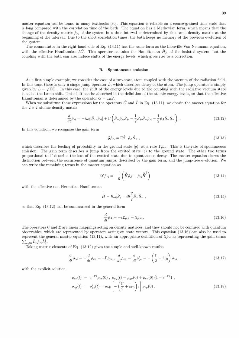
39

master equation can be found in many textbooks [30]. This equation is reliable on a coarse-grained time scale thatis long compared with the correlation time of the bath. The equation has a Markovian form, which means that thechange of the density matrix ρA of the system in a time interval is determined by this same density matrix at thebeginning of the interval. Due to the short correlation times, the bath keeps no memory of the previous evolution ofthe system.

The commutator in the right-hand side of Eq. (13.11) has the same form as the Liouville-Von Neumann equation,with the effective Hamiltonian ~G. This operator contains the Hamiltonian HA of the isolated system, but thecoupling with the bath can also induce shifts of the energy levels, which gives rise to a correction.

B. Spontaneous emission

As a first simple example, we consider the case of a two-state atom coupled with the vacuum of the radiation field.In this case, there is only a single jump operator L, which describes decay of the atom. The jump operator is simplygiven by L =

√ΓS−. In this case, the shift of the energy levels due to the coupling with the radiative vacuum state

is called the Lamb shift. This shift can be absorbed in the definition of the atomic energy levels, so that the effectiveHamiltonian is determined by the operator G = ω0Sz.

When we substitute these expressions for the operators G and L in Eq. (13.11), we obtain the master equation forthe 2× 2 atomic density matrix

d

dtρA = −iω0[Sz, ρA] + Γ

(S−ρAS+ − 1

2S+S−ρA − 1

2ρAS+S−

). (13.12)

In this equation, we recognize the gain term

GρA = ΓS−ρAS+ , (13.13)

which describes the feeding of probability in the ground state |g〉, at a rate Γρee. This is the rate of spontaneousemission. The gain term describes a jump from the excited state |e〉 to the ground state. The other two termsproportional to Γ describe the loss of the excited state due to spontaneous decay. The master equation shows thedistinction between the occurrence of quantum jumps, described by the gain term, and the jump-free evolution. Wecan write the remaining terms in the master equation as

−iLρA = − i

~

(ˆHρA − ρA

ˆH†)

(13.14)

with the effective non-Hermitian Hamiltonian

ˆH = ~ω0Sz − i~Γ2

S+S− , (13.15)

so that Eq. (13.12) can be summarized in the general form

d

dtρA = −iLρA + GρA . (13.16)

The operators G and L are linear mappings acting on density matrices, and they should not be confused with quantumobservables, which are represented by operators acting on state vectors. This equation (13.16) can also be used torepresent the general master equation (13.11), with an appropriate definition of GρA as representing the gain terms∑

ν 6=0 Lν ρAL†ν .Taking matrix elements of Eq. (13.12) gives the simple and well-known results

d

dtρee = − d

dtρgg = −Γρee ,

d

dtρeg =

d

dtρ∗ge = −

(Γ2

+ iω0

)ρeg , (13.17)

with the explicit solution

ρee(t) = e−Γtρee(0) , ρgg(t) = ρgg(0) + ρee(0)(1− e−Γt

),

ρeg(t) = ρ∗ge(t) = exp[−

(Γ2

+ iω0

)t

]ρeg(0) . (13.18)

40

pe

pe

pe

pe

t t t

t

1 1 1

1

FIG. 10: The exponential decay law is an ensemble average over many histories of an excited atom that emits a photoninstantaneously.

This shows the standard exponential decay of an excited atom by spontaneous decay. Notice that the off-diagonalelements (which are also called the optical coherences of the atom) decay at half the decay rate Γ of the excited-statepopulation. One can check that a density matrix will remain positive definite and normalized at later times whenρA(0) is positive definite and normalized.

The exponential decay law can be directly observed by measuring the emitted photon intensity for a large collectionof atoms, just as in other cases of quantum-mechanical decay processes, such as radioactive decay of nuclei. However,if we think of a single excited atom that is constantly monitored by photodetectors, all one observes is that a photonis detected at one point in time. Then we conclude that the atom has resided in the excited state |e〉 up to the timeinstant of the emission, and that it is in the ground state |g〉 from that time on. This means that the probability pe

for the atom to be in the excited state remains equal to 1 up to the emission time, and then jumps to the value 0.The exponential behavior arises only when one repeats the experiment many times, and takes the average. In

Figure 10 we sketch three typical single runs, together with the average exponential decay. The solution of the masterequation only describes the statistical average over many single runs of the experiment. This raises the question howone can reconstruct the single runs from a given master equation.

It is not difficult to see how this can be done when an experiment consists of observing the occurrence of the jumps.For this purpose we represent the formal solution of the master equation in the form (13.16) of an expansion in powersof the gain operator G, which describes the quantum jumps. The result is

ρA(t) = e−iLtρA(0)

+∫ t

0

dt1e−iL(t−t1)Ge−iLt1 ρA(0)

+∫ t

0

dt2

∫ t2

0

dt1e−iL(t2−t1)Ge−iL(t2−t1)Ge−iLt1 ρA(0)

+ . . .

= ˆρ0(t) + ˆρ1(t) + ˆρ2(t) + . . . . (13.19)

Here and in the following we use a tilde ( ) to indicate density matrices or state vectors that are not normalized, ora Hamiltonian that is not Hermitian. The first term gives the contribution to the density matrix from the jump-freeevolution, the second term gives the contribution of the single runs with precisely one jump in the time interval [0, t),etc. The integrals are over the time instants of the jumps. Furthermore, the trace of ˆρk has the significance of theprobability Pk(t) of precisely k jumps between time 0 and t, so that

Pk(t) = Tr ˆρk(t) . (13.20)

Because of the normalization of the total density matrix ρA(t), these probabilities add up to 1, as they should. Thesum in the right-hand side of Eq. (13.19) can be viewed as a weighted sum with weights Pk of normalized densitymatrices ρk = ˆρk/Pk. These can be regarded as conditional density matrices: the density matrix ρk(t) gives the state

41

for the sub-ensemble of histories where precisely k jumps have occurred. The total density matrix (13.19) can bewritten as

ρA(t) =∑

k

Pk(t)ρk(t) , (13.21)

which should be read as a decomposition in normalized contributions of subensembles corresponding to the numberof jumps. The probability W (t) = 1− P0(t) that is complementary to the zero-jump probability has the significanceof the probability that the first jump occurs before t. Its time derivative

w(t) =dW

dt= −dP0

dt(13.22)

is the waiting-time distribution, defined by the requirement that the probability that the first jump occurs betweent and t + dt is equal to w(t)dt. Note that W (t) is monotonously increasing with t, so that P0(t) is monotonouslydecreasing, and w(t) is non-negative.

In fact, in the present case of a single atom without any driving field, the atom will end up in the ground stateafter the first jump without ever getting excited again. Hence, for this special case, the expansion breaks off, and theidentity ρA(t) = ρ0(t) + ρ1(t) holds exactly. The density matrix is separated in contributions from the single runswhere no emission occurred (ρ0(t)), and the runs with one emission (ρ1(t)). When in the initial state the atom hasa non-vanishing probability pg(0) to be in the ground state, with this same probability the atom will never emit aphoton, so that P0(∞) = pg(0). Hence, the zero-jump probability P0(t) decreases from its zero-time value 1 to thelarge-time value pg(0). Conversely, the function W (t) increases from 0 to 1− pg(0) = pe(0).

Now it is rather obvious how one could numerically simulate single runs of the experiment in which spontaneousemission of a single atom is observed. We first assume an initial state of the atom, of the pure-state form ρA(0) =|ψA(0)〉〈ψA(0)|, with |ψA(0)〉 = α|e〉 + β|g〉. First, one simulates the time instant of the first emission. This can bedone by drawing a random number ξ between 0 and 1, so that the probability for a drawn value between ξ and ξ + dξis equal to dξ. The time instant t1 of the first (and only) emission is then determined by setting W (t1) = ξ. Thenthe probability for an emission time between t1 and t1 + dt1 is equal to dξ = dW = w(t1)dt1, as it should be. Whenξ > pe(0) = |α|2, no value of t1 is obtained. This happens with the probability 1− pe(0) = pg(0) = |β|2. In this case,no emission occurs at any time.

When we know at what time (if ever) a photon is emitted, the evolution is obvious. The state of the system fromtime 0 to t1 is governed by the operator −iL. Under this evolution, an initially pure state remains pure, and thedensity matrix ˆρ0(t) = exp(−iLt)ρ(0) can be written as |ψA(t)〉〈ψA(t)|, with

|ψA(t)〉 = exp(−i ˆHt/~)|ψA(0)〉 , (13.23)

for 0 ≤ t ≤ t1. Due to the non-Hermitian nature of the effective Hamiltonian ˆH, the state |ψ(t)〉 decays, and it doesnot remain normalized. The conditional density matrix ρ0(t) corresponding to the no-jump condition is then equalto |ψA(t)〉〈ψA(t)| with the normalized pure state

|ψA(t)〉 = |ψA(t)〉/√

P0(t) (13.24)

for 0 ≤ t ≤ t1. For times t after the emission time, the atom is in the ground state. The conclusion is that for thesingle run of the experiment where a photon is emitted at time t1, the atom is in the pure state |ψA(t)〉. This stateis given by Eq. (13.24) for t ≤ t1, whereas |ψA(t)〉 = |g〉 for t > t1.

Before the jump, an expression for the state |ψA(t)〉 follows from the evolution equation (13.23). This gives

|ψA(t)〉 = α exp(−1

2(iω0 + Γ)t

)|e〉+ β exp

(12iω0t

)|g〉 . (13.25)

The no-jump probability P0(t) = 〈ψA(t)|ψA(t)〉 is therefore

P0(t) = |α|2e−Γt + |β|2 . (13.26)

The state vector (13.24) provides the amplitude for the atom to be in the excited state for this single run. Thecorresponding probability pe(t) is found as

pe(t) =pe(0)e−Γt

pe(0)e−Γt + pg(0), (13.27)

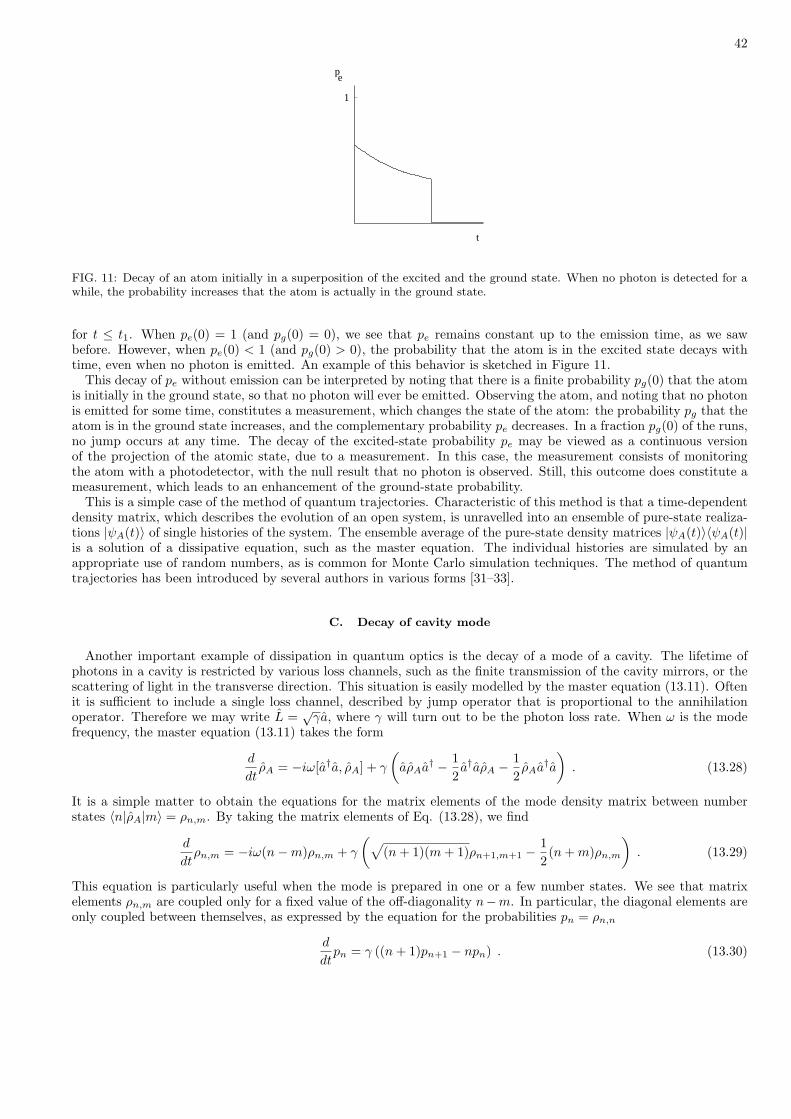
42

pe

t

1

FIG. 11: Decay of an atom initially in a superposition of the excited and the ground state. When no photon is detected for awhile, the probability increases that the atom is actually in the ground state.

for t ≤ t1. When pe(0) = 1 (and pg(0) = 0), we see that pe remains constant up to the emission time, as we sawbefore. However, when pe(0) < 1 (and pg(0) > 0), the probability that the atom is in the excited state decays withtime, even when no photon is emitted. An example of this behavior is sketched in Figure 11.

This decay of pe without emission can be interpreted by noting that there is a finite probability pg(0) that the atomis initially in the ground state, so that no photon will ever be emitted. Observing the atom, and noting that no photonis emitted for some time, constitutes a measurement, which changes the state of the atom: the probability pg that theatom is in the ground state increases, and the complementary probability pe decreases. In a fraction pg(0) of the runs,no jump occurs at any time. The decay of the excited-state probability pe may be viewed as a continuous versionof the projection of the atomic state, due to a measurement. In this case, the measurement consists of monitoringthe atom with a photodetector, with the null result that no photon is observed. Still, this outcome does constitute ameasurement, which leads to an enhancement of the ground-state probability.

This is a simple case of the method of quantum trajectories. Characteristic of this method is that a time-dependentdensity matrix, which describes the evolution of an open system, is unravelled into an ensemble of pure-state realiza-tions |ψA(t)〉 of single histories of the system. The ensemble average of the pure-state density matrices |ψA(t)〉〈ψA(t)|is a solution of a dissipative equation, such as the master equation. The individual histories are simulated by anappropriate use of random numbers, as is common for Monte Carlo simulation techniques. The method of quantumtrajectories has been introduced by several authors in various forms [31–33].

C. Decay of cavity mode

Another important example of dissipation in quantum optics is the decay of a mode of a cavity. The lifetime ofphotons in a cavity is restricted by various loss channels, such as the finite transmission of the cavity mirrors, or thescattering of light in the transverse direction. This situation is easily modelled by the master equation (13.11). Oftenit is sufficient to include a single loss channel, described by jump operator that is proportional to the annihilationoperator. Therefore we may write L =

√γa, where γ will turn out to be the photon loss rate. When ω is the mode

frequency, the master equation (13.11) takes the form

d

dtρA = −iω[a†a, ρA] + γ

(aρAa† − 1

2a†aρA − 1

2ρAa†a

). (13.28)

It is a simple matter to obtain the equations for the matrix elements of the mode density matrix between numberstates 〈n|ρA|m〉 = ρn,m. By taking the matrix elements of Eq. (13.28), we find

d

dtρn,m = −iω(n−m)ρn,m + γ

(√(n + 1)(m + 1)ρn+1,m+1 − 1

2(n + m)ρn,m

). (13.29)

This equation is particularly useful when the mode is prepared in one or a few number states. We see that matrixelements ρn,m are coupled only for a fixed value of the off-diagonality n−m. In particular, the diagonal elements areonly coupled between themselves, as expressed by the equation for the probabilities pn = ρn,n

d

dtpn = γ ((n + 1)pn+1 − npn) . (13.30)

43

It is also useful to derive the time derivative of the expectation value of an arbitrary observable QA of the mode.From the defining relation 〈QA〉 = Tr ρAQA of the mode, we obtain the identity

d

dt〈QA〉 = iω〈[a†a, QA]〉 − γ

2〈[QA, a†]a + a†[a, QA]〉 . (13.31)

When we substitute for QA the annihilation operator a or the number operator N = a†a, this equation (13.31) gives

d

dt〈a〉 = −

(iω +

γ

2

)〈a〉 ,

d

dt〈N〉 = −γ〈N〉 . (13.32)

Hence, these expectation values obey closed equations, with the solutions

〈a(t)〉 = exp(−(iω +

γ

2)t

)〈a(0)〉 , 〈N(t)〉 = exp (−γt) 〈N(0)〉 . (13.33)

Hence the expectation value of the annihilation operator, which is the quantum analogue of the classical field am-plitude, decays at the rate γ/2. The expectation value of the number operator, which is the quantum version of theintensity, decays at the rate γ.

For an arbitrary density matrix of the mode we introduce the quantity

V = 〈a†a〉 − 〈a†〉〈a〉 , (13.34)

which has the significance of the variance of the complex field amplitude. When the mode is in a coherent state, sothat the density matrix is ρA = |z〉〈z| for some value of z, the variance V is obviously zero. The opposite is also true:when the variance vanishes, the mode must be in a coherent state. This is easily proven when we write the densitymatrix in the diagonal form ρ =

∑n pn|ψn〉〈ψn|, as a classical average over projection operators. When we denote

the expectation of the annihilation operator as z, the variance can be expressed as

V =∑

n

pn〈ψn|(a† − z∗)(a− z)|ψn〉 . (13.35)

Since each one of the summands is non-negative, they must all be zero when V is zero. This means that each state|ψn〉 for which the probability pn is non-zero must be eigenstate of a with eigenvalue z, which is the coherent state|z〉.

From the expectation values (13.33) it is obvious that for an arbitrary initial density matrix this variance decaysuniformly as V (t) = V (0) exp(−Γt). In the special case that the mode is initially in a coherent state |z0〉, thevariance is zero, and therefore the mode is in a coherent state at all times. From Eq. (13.33) we conclude that thetime-dependent density matrix is then ρA(t) = |z(t)〉〈z(t)| with z(t) = z0 exp(−iωt− γt/2).

Finally, we consider the case that the mode is initially in a superposition of two strongly different coherent states,so that ρA(0) = |ψ(0)〉〈ψ(0)|, with

|ψ(0)〉 ≈ 1√2

(|z1〉+ |z2〉) , (13.36)

with |z1 − z2| À 1. The overlap between the two coherent states is very small, so that they can be treated as nearlyorthonormal states. A coherent state has a classical nature. This state |ψ0〉 is a superposition of two states thatare macroscopically different. Such a state is called a Schrodinger cat state, in reference to the famous picture ofSchrodinger of a cat that is in a superposition of a state of being alive, and a state of being dead. This was intended toillustrate the absurdity of the superposition principle when applied to macroscopic states. The initial density matrixcan be expressed as

ρA(0) ≈ 12

(|z1〉〈z1|+ |z2〉〈z2|+ |z1〉〈z2|+ |z2〉〈z1|) . (13.37)

The evolution of the two diagonal terms is known, since, as discussed above, these evolve as pure coherent states.The evolution of the off-diagonal terms can be estimated by substituting them in the master equation (13.28). Forlarge values of |z1 − z2|, the decay rate of the off-diagonal terms is dominated by a contribution γ|z1 − z2|2/2. Theoff-diagonality between largely separated coherent states decays very much faster than the decay rate γ of the cavity.After a very short time, the off-diagonal terms have disappeared, and the density matrix is given by

ρA ≈ 12

(|z1〉〈z1|+ |z2〉〈z2|) . (13.38)

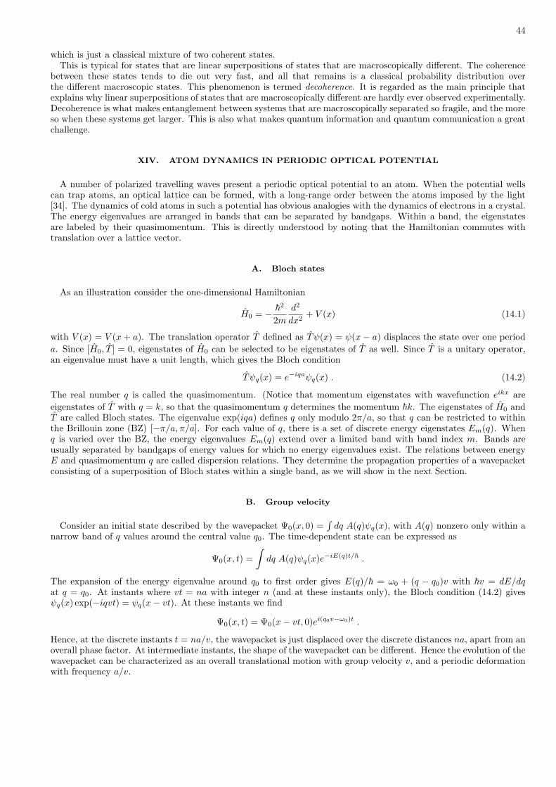
44

which is just a classical mixture of two coherent states.This is typical for states that are linear superpositions of states that are macroscopically different. The coherence

between these states tends to die out very fast, and all that remains is a classical probability distribution overthe different macroscopic states. This phenomenon is termed decoherence. It is regarded as the main principle thatexplains why linear superpositions of states that are macroscopically different are hardly ever observed experimentally.Decoherence is what makes entanglement between systems that are macroscopically separated so fragile, and the moreso when these systems get larger. This is also what makes quantum information and quantum communication a greatchallenge.

XIV. ATOM DYNAMICS IN PERIODIC OPTICAL POTENTIAL

A number of polarized travelling waves present a periodic optical potential to an atom. When the potential wellscan trap atoms, an optical lattice can be formed, with a long-range order between the atoms imposed by the light[34]. The dynamics of cold atoms in such a potential has obvious analogies with the dynamics of electrons in a crystal.The energy eigenvalues are arranged in bands that can be separated by bandgaps. Within a band, the eigenstatesare labeled by their quasimomentum. This is directly understood by noting that the Hamiltonian commutes withtranslation over a lattice vector.

A. Bloch states

As an illustration consider the one-dimensional Hamiltonian

H0 = − ~2

2m

d2

dx2+ V (x) (14.1)

with V (x) = V (x + a). The translation operator T defined as Tψ(x) = ψ(x− a) displaces the state over one perioda. Since [H0, T ] = 0, eigenstates of H0 can be selected to be eigenstates of T as well. Since T is a unitary operator,an eigenvalue must have a unit length, which gives the Bloch condition

Tψq(x) = e−iqaψq(x) . (14.2)

The real number q is called the quasimomentum. (Notice that momentum eigenstates with wavefunction eikx areeigenstates of T with q = k, so that the quasimomentum q determines the momentum ~k. The eigenstates of H0 andT are called Bloch states. The eigenvalue exp(iqa) defines q only modulo 2π/a, so that q can be restricted to withinthe Brillouin zone (BZ) [−π/a, π/a]. For each value of q, there is a set of discrete energy eigenstates Em(q). Whenq is varied over the BZ, the energy eigenvalues Em(q) extend over a limited band with band index m. Bands areusually separated by bandgaps of energy values for which no energy eigenvalues exist. The relations between energyE and quasimomentum q are called dispersion relations. They determine the propagation properties of a wavepacketconsisting of a superposition of Bloch states within a single band, as we will show in the next Section.

B. Group velocity

Consider an initial state described by the wavepacket Ψ0(x, 0) =∫

dq A(q)ψq(x), with A(q) nonzero only within anarrow band of q values around the central value q0. The time-dependent state can be expressed as

Ψ0(x, t) =∫

dq A(q)ψq(x)e−iE(q)t/~ .

The expansion of the energy eigenvalue around q0 to first order gives E(q)/~ = ω0 + (q − q0)v with ~v = dE/dqat q = q0. At instants where vt = na with integer n (and at these instants only), the Bloch condition (14.2) givesψq(x) exp(−iqvt) = ψq(x− vt). At these instants we find

Ψ0(x, t) = Ψ0(x− vt, 0)ei(q0v−ω0)t .

Hence, at the discrete instants t = na/v, the wavepacket is just displaced over the discrete distances na, apart from anoverall phase factor. At intermediate instants, the shape of the wavepacket can be different. Hence the evolution of thewavepacket can be characterized as an overall translational motion with group velocity v, and a periodic deformationwith frequency a/v.

45

C. Wannier states

We consider the lowest energy band, suppressing the band index m. The Bloch state vector with wave functionψq(x) is denoted as |q〉. We choose the normalization as

〈q|q′〉 =∫ ∞

−∞dx ψ∗q (x) ψq′(x) = δ(q − q′)

for q, q′ in BZ. We introduce the Fourier transforms of the Bloch states as

|n〉 =√

a

2π

∫

BZ

dq|q〉e−iqna , or inversely |q〉 =√

a

2π

∑n

|n〉einqa .

The states |n〉 defined this way are called the Wannier states. They obey the normalization condition 〈n|n′〉 = δnn′ ,which shows that the Wannier states are localized. The Bloch condition (14.2) applied to the definition of Wannierstates gives the identity T |n >= |n+1〉, so that the Wannier wavefunctions obey the identity 〈x−a|n〉 = φn(x−a) =φn+1(x) = 〈x|n+1〉. Because H0 and T commute, we find T †H0T = H0, or 〈n|H0|n′〉 = 〈n+1|H0|n′+1〉. This provesthat the coefficients Em = 〈n − m|H|n〉 are independent of n. The expansion of the Bloch states in the Wannierstates then gives H0|q〉 = E(q)|q〉 with

E(q) =∑m

Emeimqa . (14.3)

Hence the coupling coefficients between subsequent neighboring wells are the Fourier coefficients of the dispersionrelation E(q). The series of Wannier states can be defined for each energy band, and they define an orthogonaldiscrete basis of the band.

When the potential V (x) consists of potential wells at distance a that are sufficiently deep, we may assume thatthe ground states in each well are only coupled to the ground state of the nearest neighbors. This specifies thetight-binding model, with Em = 0 for |m|〉1. Then the Wannier state |n〉 is the ground state in the well n (locatedat x = na), which is coupled only to the ground state in neighboring wells n ± 1. The Wannier wavefunctions canbe assumed real, so that E−1 = E∗

1 = E1. From the Fourier expansion (14.3) of the dispersion relation we then findE(q) = E0 + 2E1 cos(qa).

D. Bloch oscillations

When a particle is subjected to a spatially uniform force, its momentum grows linearly in time. When the uniformforce is applied to a particle in a periodic potential with well-separated energy bands, the wavepacket will undergo aperiodic motion, termed Bloch oscillation. This can be demonstrated by considering the Hamiltonian H = H0 − Fx,with H0 given by (14.1). The commutator of the Hamiltonian H with the displacement operator T is then [H, T ] =−[Fx, T ] = −(aF/~)T , which gives

eiHt/~T e−iHt/~ = e−iaFt/~T .

Hence, when the initial state |Ψ(0)〉 = |q0〉 is a Bloch state, the time-dependent state obeys the eigenvalue relation

T |Ψ(t)〉 = T e−iHt/~|q0〉 = e−iaFt/~e−iHt/~T |q0〉 = e−iq0a−iaFt/~|Ψ(t)〉 .

This shows that |Ψ(t)〉 is eigenvector of T with the time-dependent eigenvalue q(t) = q0 + Ft/~. When the energybands are well separated, interband coupling is negligible, which means that, apart from a phase factor, |Ψ(t) mustbe equal to the Bloch state |q(t)〉 in the same band as |q0〉, which we took to be the lowest energy band. Hence aftera time τ = 2π~/(aF ), the time-dependent state has traversed the Brillouin zone, and |Ψ(t)〉 is again proportional to|q0〉. Moreover, the phase factor exp(−iα) picked up after one period τ is independent of the initial value q0. Hencewhen the initial state is the superposition |Ψ(0)〉 =

∫dq0 A(q0)|q0〉 of the Bloch states, the time-dependent state

|Ψ(t)〉 is a similar superposition of states |q0 + Ft/~〉, but with a phase factor that depends on q0. After one periodτ , we find that |Ψ(τ)〉 = e−iα|Ψ(0)〉. Hence a uniform force leads to an oscillatory behavior of the wavepacket withperiod τ = 2π~/(aF ). The trajectory of the packet is determined by the periodic group velocity v(t) = 1

~∂E/∂q,evaluated at q = q(t).

46

Bloch oscillations have been predicted for electrons in a crystal in a uniform electric field [35], but they have neverbeen observed for electrons. Observation of this oscillatory behavior of atoms in an optical lattice has recently beenaccomplished [36]. The uniform force has been mimicked by a time-dependent variation of the frequency difference oftwo counterpropagating traveling waves, which creates a standing wave in a reference frame in uniform accelerationThe force F is just the inertial force in this moving frame in which the Bloch oscillations occur.

[1] C. Cohen-Tannoudji, J. Dupont-Roc et G. Grynberg, Photons et Atomes (InterEditions CNRS, Paris, 1987); Photons andAtoms (Wiley, New York, 1989).

[2] S. J. van Enk and G. Nienhuis, J. Mod. Opt. 41, 963 (1994)[3] D. Lenstra and L. Mandel, Phys. Rev A 26, 3428 (1982).[4] S. J. van Enk and G. Nienhuis, Europhys. Lett. 25, 497 (1994).[5] P. A. M. Dirac, Proc. R. Soc. A 114, 243 (1927).[6] S. M. Barnett, and D. T. Pegg, J. Mod. Opt. 36, 7 (1989).[7] E. Wigner, Phys. Rev. 40, 749 (1932).[8] M. Born and E. Wolf, Principles of Optics (Pergamon, New York, 1980).[9] J. Schwinger, Quantum Theory of Angular Momentum (Academic Press, New York, 1965).

[10] F. T. Arecchi, E. Courtens, R. Gilmose and H. Thomas, Phys. Rev A 6, 2211 (1972).[11] M. Lax, W. H. Louisell and W. B. McKnight, Phys. Rev. A 11, 1365 (1975).[12] H. A. Haus, Waves and Fields in Optoelectronics (Prentice Hall, Englewood Cliffs, NJ, 1984).[13] S. J. van Enk and G. Nienhuis, Opt. Commun. 94, 147 1992.[14] L. Allen, M. W. Beijersbergen, R. J. C. Spreeuw, and J. P. Woerdman, Phys. Rev. A 45, 8185 (1992).[15] J. M. Jauch and F. Rohrlich, The Theory of Photons and Electrons Springer, Berlin, 1976.[16] J. W. Simmons and M. J. Guttmann, States, Waves and Particles (Addison-Wesley, Reading Mass. 1970).[17] A. E. Siegman, Lasers (University Science Books, Sausalito, CA, 1986).[18] Z. Bomzon, G. Biener, V.K leiner and E. Hasman, Opt. Lett. 27, 285 (2002).[19] A. Niv, G. Biener, V. Kleiner and E. Hasman, Opt. Lett. 28, 510, 2003.[20] G. Nienhuis and L. Allen, Phys. Rev. A 48, 48 (1993).[21] G. Nienhuis and J. Visser, J. Opt. A: Pure Appl. Opt. 6, S248 (2004).[22] D. Stoler, J. Opt. Soc. Am. 71, 334 (1981).[23] S. J. M. Habraken and G. Nienhuis, Phys. Rev. A 75, 033819 (2007).[24] J. Visser and G. Nienhuis, Phys. Rev. A 70, 013809 (2004).[25] A. Einstein, B. Podolsky and N. Rosen, Phys. Rev. 47, 777 (1935).[26] D.M. Greenberger, M.A. Horne, A. Shimony and A. Zeilinger, Am. J. Phys. 58, 1131 (1990).[27] G. Nogues, A. Rauschenbeutel, S. Osnaghi, M. Brune, J.M. Raimond and S. Haroche, Nature 400, 239 (1999).[28] A. Rauschenbeutel, G. Nogues, S. Osnaghi, P. Bertet, M. Brune, J.M. Raimond and S. Haroche, Science 288, 2024 (2000).[29] M. Brune, S. Haroche, J.M. Raimond, L. Davidovich and N. Zagury, Phys. Rev A 45, (1992) 5193.[30] L. Mandel and E. Wolf, Optical Coherence and Quantum Optics (Cambridge University Press, Cambridge, 1995).[31] J. Dalibard, Y Castin and K. Mølmer, Phys. Rev. Lett. 68, 580 (1992).[32] R. Dum, P. Zoller and H. Ritsch, Phys. Rev. A 45, 4879 (1992).[33] H.J. Carmichael, An Open System Approach to Quantum Optics (Springer, Berlin, 1993).[34] K. I. Petsas, A. B. Coates and G. Grynberg, Phys. Rev. A 50, 5173 (1994).[35] F. Bloch, Z. Phys.52, 555 (1927).[36] M. Ben Dahan, E. Peik, J. Reichel, Y. Castin and C. Salomon, Phys. Rev. Lett. 76, 4508 (1996).