
Operations Planning and Scehduling -...
44
14 – 1 Planning and Scheduling Operations in Dynamic Supply Chain Sung Joo Bae Assistant Professor Yonsei University
Transcript of Operations Planning and Scehduling -...

14 – 1
Planning and Scheduling Operations in Dynamic Supply Chain
Sung Joo Bae Assistant Professor Yonsei University
14 – 2
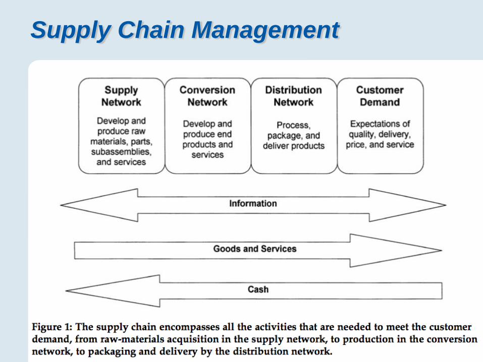
Supply Chain Management

14 – 3
East Coast West Coast East Europe West Europe Retail
USA Ireland Distribution
centers
Manufacturer Ireland
Assembly
Germany Mexico USA Tier 1 Major
subassemblies
Germany Mexico USA China Tier 2 Components
Supply Chains
Poland USA Canada Australia Malaysia Tier 3 Raw
materials
Figure 9.2 – Supply Chain for a Manufacturing Firm

14 – 4
Supply Chain Dynamics
Bullwhip effect
Variability of the order quantities increase as you proceed upstream
Upstream members must react to the demand
Slightest change in customer demand can ripple through the entire chain
External causes: volume changes, service/product mix changes, late deliveries
Internal causes: engineering changes, order batching, new svc/prod introductions, svc/prod promotions

14 – 5
Supply Chain Dynamics
Consumers’ daily
demands
Retailers’ daily orders to
manufacturer
Manufacturer’s weekly orders to package supplier
Package supplier’s weekly orders to
cardboard supplier 9,000
7,000
5,000
3,000
0
Ord
er
qu
an
tity
Month of April
Day 1 Day 30 Day 1 Day 30 Day 1 Day 30 Day 1 Day 30
Figure 10.2 – Supply Chain Dynamics for Facial Tissue

14 – 6
Across the Organization
Operations planning and scheduling is the process of making sure that demand and supply plans are in balance at all levels
Sales and operations planning and scheduling
Requires managerial inputs from all of the firm’s functions
Each function is affected by the plan

14 – 7
Across the Organization
TABLE 14.1 | TYPES OF PLANS WITH OPERATIONS PLANNING AND | SCHEDULING
Term Definition
Sales and operations plan (S&OP)
A time-phased plan (projected for several months or quarters) of future aggregate resource levels (production rates, workforce levels, and inventory holdings) so that supply is in balance with demand throughout the organization
Aggregate plan Another term for the sales and operations plan
Production plan A manufacturing firm’s sales and operations plan that centers on production rates and inventory holdings
Staffing plan A sales and operations plan for a service firm, which centers on staffing and on other human resource-related factors
Resource plan An intermediate, more detailed, step in the planning process that lies between S&OP and scheduling
Schedule A detailed plan that allocates resources over shorter time horizons to accomplish specific tasks

14 – 8
Aggregation
Targets and resources used for creating effective schedules
Product families: according to similar demand requirements (e.g. 12 bicycles into 2 PF – mountain and road bikes)
Workforce: (e.g. A single group for two PF, or two groups – full-time and part-time)
Time: planning horizon – usually one year, but quarter, season can be used as well
The relationship of operations plans and schedules to other plans
A business plan: projected statement of income, costs, and profits
An annual plan or financial plan
Resource planning
The lowest planning level is scheduling
Stages in Planning and Scheduling

14 – 9
Stages in Planning and Scheduling
Business or annual plan
• Employee and equipment schedules • Production order schedules • Purchase order schedules
Scheduling
• Employee schedules • Facility schedules • Customer schedules
Scheduling
• Master production schedule • Material requirements planning
Resource Planning (manufacturing)
• Workforce schedule • Materials and facility resources
Resource Planning (services)
Sales Plan
Operations Plan
Sales and Operations Plan
Forecasting
Operations strategy
Capacity/Constraint management
Figure 14.1 – The Relationship of Sales and Operations Plans and Schedules to Other Plans
Dynamic

14 – 10
Matching supply with demand becomes challenging when forecasts call for uneven demand patterns
Demand management: the process of changing demand patterns using one or more demand options
Managing Demand

14 – 11
Managing Demand
TABLE 14.2 | DEMAND AND SUPPLY OPTIONS FOR | OPERATIONS PLANNING AND SCHEDULING
Demand Options
Complementary products
Prod/svc that has similar resource requirement, but different demand cycles
(e.g. city parks used for ice skating for the winter months)
Promotional pricing Creative pricing for evening out the
demand (e.g. Low price hotel rooms during
off-season, winter clothing in summer)
Prescheduled appointments
Timely customer service and high utilization
of service personnel through scheduled
services
Reservations
More lead time and ability to level demand

14 – 12
Managing Demand
TABLE 14.2 | DEMAND AND SUPPLY OPTIONS FOR | OPERATIONS PLANNING AND SCHEDULING
Demand Options
Revenue management
Process of varying price at the right time for different
customer segments to maximize revenues with the
existing supply
(e.g. airline’s varying prices in the reservation system)
Backlogs Accumulation of customer orders that a manufacturer
has promised future delivery.
(e.g. Airplane manufacturers such as Boeing & firms
with customized products and make-to-order strategy
uses backlogs)
Backorders Customer order that cannot be filled immediately but
as soon as possible
Stockouts Order is lost due to the incapability to meet the
demand

14 – 13
Managing Demand
TABLE 14.2 | DEMAND AND SUPPLY OPTIONS FOR | OPERATIONS PLANNING AND SCHEDULING
Supply Options
Anticipation inventory
Inventory level increased during light demand periods
for preparing for heavy demand periods
Workforce adjustment (hiring or layoffs)
Only available when the skill level doesn’t matter
much. In some industries such as tourism and
agriculture, seasonal hiring and layoffs are common
Workforce utilization (overtime and undertime)
Longer or shorter working hours. Mostly with extra
pay
Part-time workers and subcontractors
Low skill areas

14 – 14
Aggregate plan
Sales and Operations Planning(S&OP)
Supplier capabilities
Storage capacity
Materials availability
Materials
Current machine capacities
Plans for future capacities
Workforce capacities
Current staffing level
Operations
New products
Product design changes
Machine standards
Engineering
Labor-market conditions
Training capacity
Human resources
Cost data
Financial condition
of firm
Accounting and finance
Customer needs
Demand forecasts
Competition behavior
Distribution and marketing
Figure 14.2 – Managerial Inputs from Functional Areas to Sales and Operations Plans

14 – 15
Sales and Operations Plans
Planning strategies
Chase strategy
Hiring and laying off employees to match the demand forecast over the planning horizon
Pros: No inventory management, overtime or undertime
Cons: Loss of productivity and quality
Level strategy
Keep the workforce constant
Use overtime, undertime, and vacation planning to match the demand forecast
Mixed strategy

14 – 16
Sales and Operations Plans
TABLE 14.3 | TYPES OF COSTS WITH SALES AND OPERATIONS PLANNING
Cost Definition
Regular time Regular-time wages plus benefits and pay for vacations
Overtime Wages paid for work beyond the normal workweek exclusive of fringe benefits
Hiring and layoff Cost of advertising jobs, interviews, training programs, scrap caused by inexperienced employees, exit interviews, severance pay, and retraining
Inventory holding Capital, storage and warehousing, insurance, and taxes
Backorder and stockout
Costs to expedite past-due orders, potential cost of losing a customer

14 – 17
Sales and Operations Plans
Finalize and
communicate 6
Executive S&OP
meeting 5
Consensus meeting
4
Update S&OP spreadsheets
3
Demand planning
2
Gather data
1
Six steps in the sales and operations planning process

14 – 18
Figure 14.3 – Sales and Operations Plan for Make-to-Stock Product Family
Sales and Operations Plans
14 – 19
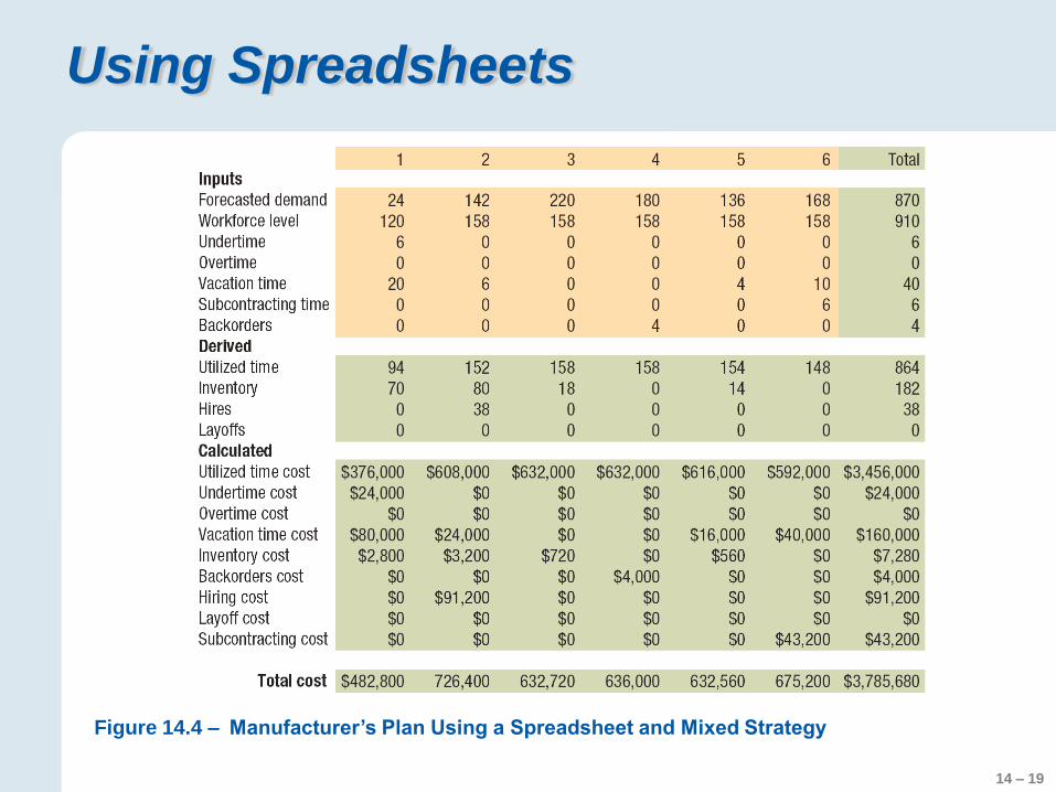
Using Spreadsheets
Figure 14.4 – Manufacturer’s Plan Using a Spreadsheet and Mixed Strategy

14 – 20
HMC’s Production Planning & Scheduling
5 common causes of misalignment in supply chain
Functional organizations managed independently
Functional objectives conflict
Ineffective information systems
Lack of customer focus
Different needs of the customers not recognized within the supply chain

14 – 21
HMC’s Production Planning & Scheduling
A large-volume-production requirement with a large variety of small-lot make-to-order requirements involving thousands of suppliers and dealers
400 first-tier suppliers, 2500 second-tier suppliers (many foreign suppliers)
Production-and-sales-control (P/SC) department: centralized coordinating group with an integrated perspective
Synchronizing sales and plant capacity
Balancing requests from the domestic and export sales departments
Dealing with shortages and excesses of inventory due to schedule changes
Coordinating the new product introductions or part changes
Synchronizing order-launching and delivery activities

14 – 22

14 – 23
HMC’s Production Planning & Scheduling
Structural problems
Initially, authority and responsibility for the planning process were not well defined
Managing information flows
Environmental Problems
Rapidly changing internal/external conditions: success in NA, and Korean market
Behavioral problems
Senior managers’ frequent changes in production plan
Area representatives behaving based on their own performance expectations in each area (sub-optimization problem)
Task responsibility (of developing and providing data)

14 – 24
Video Case

14 – 25
The End

14 – 26
Using Spreadsheets
Figure 14.4 – Manufacturer’s Plan Using a Spreadsheet and Mixed Strategy

14 – 27
Using Spreadsheets
Figure 14.4 – Manufacturer’s Plan Using a Spreadsheet and Mixed Strategy

14 – 28
Using Spreadsheets
Figure 14.4 – Manufacturer’s Plan Using a Spreadsheet and Mixed Strategy

14 – 29
Using Chase and Level Strategies
EXAMPLE 14.1
A large distribution center must develop a staffing plan that minimizes total costs using part-time stockpickers
First level strategy that meets demand with the minimum use of undertime and not consider vacation scheduling
Each part-time employee can work a maximum of 20 hours per week on regular time
Instead of paying undertime, each worker’s day is shortened during slack periods and overtime can be used during peak periods
1 2 3 4 5 6 Total
Forecasted demand 6 12 18 15 13 14 78

14 – 30
Using Chase and Level Strategies
Currently, 10 part-time clerks are employed. They have not been subtracted from the forecasted demand shown. Constraints and cost information are as follows:
a. The size of training facilities limits the number of new hires in any period to no more than 10.
b. No backorders are permitted.
c. Overtime cannot exceed 20 percent of the regular-time capacity in any period. The most that any part-time employee can work is 1.20(20) = 24 hours per week.
d. The following costs can be assigned:
Regular-time wage rate $2,000/time period at 20 hrs/week
Overtime wages 150% of the regular-time rate
Hires $1,000 per person
Layoffs $500 per person

14 – 31
Using Chase and Level Strategies
SOLUTION
a. Chase Strategy
This strategy simply involves adjusting the workforce as needed to meet demand, as shown in Figure 14.5. Rows in the spreadsheet that do not apply (such as inventory and vacations) are hidden. The workforce level row is identical to the forecasted demand row. A large number of hirings and layoffs begin with laying off 4 part-time employees immediately because the current staff is 10 and the staff level required in period 1 is only 6. However, many employees, such as college students, prefer part-time work. The total cost is $173,500, and most of the cost increase comes from frequent hiring and layoffs, which add $17,500 to the cost of utilized regular-time costs.

14 – 32
Using Chase and Level Strategies
Figure 14.5 – Spreadsheet for Chase Strategy

14 – 33
Using Chase and Level Strategies
b. Level Strategy
In order to minimize undertime, the maximum use of overtime possible must occur in the peak period. For this particular level strategy (other workforce options are possible), the most overtime that the manager can use is 20 percent of the regular-time capacity, w, so
A 15-employee staff size minimizes the amount of undertime for this level strategy. Because the staff already includes 10 part-time employees, the manager should immediately hire 5 more. The complete plan is shown in Figure 14.6. The total cost is $164,000.
1.20w = 18 employees required in peak period (period 3)
w = = 15 employees 18
1.20

14 – 34
Using Chase and Level Strategies
Figure 14.6 – Spreadsheet for Level Strategy

14 – 35
Application 14.1
The Barberton Municipal Division of Road Maintenance is charged with road repair in the city of Barberton and surrounding area. Cindy Kramer, road maintenance director, must submit a staffing plan for the next year based on a set schedule for repairs and on the city budget. Kramer estimates that the labor hours required for the next four quarters are 6,000, 12,000, 19,000, and 9,000, respectively. Each of the 11 workers on the workforce can contribute 520 hours per quarter. Overtime is limited to 20 percent of the regular-time capacity in any quarter. Subcontracting is not permitted.
Payroll costs are $6,240 in wages per worker for regular time worked up to 520 hours, with an overtime pay rate of $18 for each overtime hour. Although unused overtime capacity has no cost, unused regular time is paid at $12 per hour. The cost of hiring a worker is $3,000, and the cost of laying off a worker is $2,000.

14 – 36
Application 14.1
Use a chase strategy for the Barberton Municipal Division that varies the workforce level without using overtime. Undertime should be minimized, except for the minimal amount mandated because the quarterly requirements are not integer multiples of 520 hours. (Students complete highlighted sections)

14 – 37
Quarter
1 2 3 4 Total
Forecasted demand (hrs)
6,000 12,000 19,000 9,000 46,000
Workforce level (workers)
12 24 37 18 91
Undertime (hours) 240 480 240 360 1,320
Overtime (hours) 0 0 0 0 0
Utilized time (hours)
6,000 12,000 19,000 9,000 46,000
Hires (workers) 1 12 13 19 26
Layoffs (workers) 0 0 0 0 19
Application 14.1

14 – 38
Application 14.1
What is the total cost of this plan?
Costs per Quarter
1 2 3 4 Total
Utilized time $72,000 $552,000
Undertime 2,880 15,840
Overtime 0 0
Hires 3,000 78,000
Layoffs 0 38,000
Total Cost $683,840
$144,000
5,760
0
36,000
0
$228,000
2,880
0
39,000
0
$108,000
4,320
0
0
38,000

14 – 39
Application 14.2
Find a level plan for the Barberton Municipal Division that allows no delay in road repair and minimizes undertime. Overtime can be used to its limits in any quarter. Given that the demand peaks in quarter 3, we get:
1.20w =
w = 30.45 or 31 employees
36.54 employee-period equivalents 19,000
520 =

14 – 40
Quarter
1 2 3 4 Total
Forecasted
demand (hrs)
6,000 12,000 19,000 9,000 46,000
Workforce level
(workers)
31
Undertime (hours) 10,120
Overtime (hours) 0
Utilized time
(hours)
6,000
Hires (workers) 20
Layoffs (workers) 0
Application 14.2
31
4,120
0
12,000
0
0
31
0
2,880
16,120
0
0
31
7,120
0
9,000
0
0
124
21,360
2,880
43,120
20
0

14 – 41
Costs per Quarter
1 2 3 4 Total
Utilized time $72,000 $517,440
Undertime 121,440 256,320
Overtime 0 51,840
Hires 60,000 60,000
Layoffs 0 0
Total Cost $885,600
Application 14.2
What is the total cost of this level workforce plan?
$108,000
85,440
0
0
0
$193,440
0
51,840
0
0
$144,000
49,440
0
0
0

14 – 42
Application 14.3
A mixed strategy considers and implements a fuller range of reactive alternatives than any one “pure” strategy.
Now propose a plan of your own for the Barberton Municipal Division. Use the chase strategy as a base, but find a way to decrease the cost of hiring and layoffs by selectively using some overtime. (Students complete highlighted sections)

14 – 43
Quarter
1 2 3 4 Total
Forecasted demand 6,000 12,000 19,000 9,000 46,000
Workforce level
Undertime (hours)
Overtime (hours)
Utilized time (hours)
Hires (workers)
Layoffs (workers)
Application 14.3
12
240
0
6,000
1
0
85
1,080
2,880
43,120
20
13
24
480
0
12,000
12
0
31
0
2,880
16,120
7
0
18
360
0
9,000
0
13
Several solutions are possible. The key idea in creating this one is hiring only 7 employees in quarter 3, while using overtime to its maximum limit and eliminating undertime for that quarter. Hiring fewer in quarter 3 allows the number of layoffs in quarter 4 to drop to only 13, down from 19.

14 – 44
Costs per Quarter
1 2 3 4 Total
Utilized time $72,000 $144,000 $193,440 $108,000 $517,440
Undertime
Overtime
Hires
Layoffs
Total Cost
Application 14.3
What is the cost of your mixed strategy plan?
12,960
51,840
60,000
26,000
$668,240
2,880
0
3,000
0
5,760
0
36,000
0
0
51,840
21,000
0
4,320
0
0
26,000