Operations-Oriented Performance Measures for Freeway ... · Performing Organization Report No. ......

Technical Report Documentation . Report No. FHWA/TX-08/0-5292-2

2. Government Accession No.

3. Recipient's Catalog No.

4. Title and Subtitle OPERATIONS-ORIENTED PERFORMANCE MEASURES FOR

REEWAY MANAGEMENT SYSTEMS: FINAL REPORT F

5. Report Date February 2008 Published: December 2008 6. Performing Organization Code

7. Author(s) Robert E. Brydia, Stephen P. Mattingly, Melanie L. Sattler, and

uttawit Upayokin A

8. Performing Organization Report No. Report No. 0-5292-2

9. Performing Organization Name and Address Texas Transportation Institute The Texas A&M University System College Station, Texas 77843-3135

10. Work Unit No. (TRAIS) 11. Contract or Grant No. Project 0-5292

12. Sponsoring Agency Name and Address Texas Department of Transportation Research and Technology Implementation Office P.O. Box 5080 A ustin, Texas 78763-5080

13. Type of Report and Period Covered Technical Report: September 2006 to August 2007 14. Sponsoring Agency Code

15. Supplementary Notes Project performed in cooperation with the Texas Department of Transportation and the Federal Highway Administration. Project Title: Using Operations-Oriented Performance Measures to Support Freeway Management Systems URL: http://tti.tamu.edu/documents/0-5292-2.pdf 16. Abstract This report describes the second and final year activities of the project titled “Using Operations-Oriented Performance Measures to Support Freeway Management Systems.” Work activities included developing a prototype system architecture for testing the use of performance measures in real-time. Outputs from this effort included operator’s screens, a prototype database, and a concept of operations for using the real-time measures. Additional work showcased the application of a multi-criterion screening approach to the selection of competing performance measures. 17. Key Words Performance Measurement, Operations, Emissions

18. Distribution Statement No restrictions. This document is available to the public through NTIS: National Technical Information Service Springfield, Virginia 22161 http://www.ntis.gov

19. Security Classif.(of this report) Unclassified

20. Security Classif.(of this page) Unclassified

21. No. of Pages 98

22. Price

Form DOT F 1700.7 (8-72) Reproduction of completed page authorized

http://tti.tamu.edu/documents/0-5292-2.pdf

http://www.ntis.gov

OPERATIONS-ORIENTED PERFORMANCE MEASURES FOR FREEWAY MANAGEMENT SYSTEMS: FINAL REPORT

by

Robert E. Brydia Associate Research Scientist

Texas Transportation Institute

Dr. Stephen P. Mattingly Assistant Professor

University of Texas at Arlington

Dr. Melanie L. Sattler Assistant Professor


and

Auttawit Upayokin Graduate Assistant


Report 0-5292-2 Project 0-5292

Project Title: Using Operations-Oriented Performance Measures to Support Freeway Management Systems

Performed in cooperation with the

Texas Department of Transportation and the

Federal Highway Administration

February 2008 Published: December 2008

TEXAS TRANSPORTATION INSTITUTE

The Texas A&M University System College Station, Texas 77843-3135

DISCLAIMER

This research was performed in cooperation with the Texas Department of Transportation

(TxDOT) and the Federal Highway Administration (FHWA). The contents of this report reflect

the views of the authors, who are responsible for the facts and the accuracy of the data presented

herein. The contents do not necessarily reflect the official view or policies of the FHWA or

TxDOT. This report does not constitute a standard, specification, or regulation. The researcher in

charge of this project was Robert E. Brydia.

v

vi

ACKNOWLEDGMENTS

This project was conducted in cooperation with TxDOT and FHWA. The authors

gratefully acknowledge the contributions of numerous persons who made the successful

completion of this guidebook possible.

Program Coordinator • Al Kosik, P.E., Traffic Operations Division, TxDOT

Project Director • Fabian Kalapach, P.E., Traffic Operations Division, TxDOT

Project Monitoring Committee • Charles Koonce, P.E., Austin District, TxDOT RTI Engineer • Wade Odell, P.E., Research and Technology Implementation Office, TxDOT Contract Specialist • Sandra Kaderka, Research and Technology Implementation Office, TxDOT

TABLE OF CONTENTS

Page LIST OF FIGURES ..................................................................................................................... ix LIST OF TABLES ........................................................................................................................ x CHAPTER 1: REVIEW OF YEAR ONE RESEARCH ........................................................... 1

PROJECT GOALS ..................................................................................................................... 1 LEVELS OF OPERATIONAL PERFORMANCE MEASUREMENT .................................... 1 STATE OF THE PRACTICE – OPERATIONS ........................................................................ 3 EMISSIONS PERFORMANCE MEASURES........................................................................... 4 YEAR TWO PROJECT GOALS ............................................................................................... 5

Operations ............................................................................................................................... 5 Emissions ................................................................................................................................ 5

CHAPTER 2: REAL-TIME PERFORMANCE MEASUREMENT FOR OPERATIONS .. 7 NTOC PERFORMANCE MEASURES ..................................................................................... 7 MEASURES FOR USE IN REAL-TIME PROTOTYPE TESTING ........................................ 8 SYSTEM ARCHITECTURE FOR REAL-TIME TESTING .................................................... 8 CALCULATION METHODOLOGY FOR TRAVEL TIME-LINK ......................................... 9 CALCULATION METHODOLOGY FOR EXTENT OF CONGESTION – SPATIAL ........ 10

CHAPTER 3: COMPONENTS OF SYSTEM ARCHITECTURE ....................................... 13 VISSIM SIMULATION MODEL ............................................................................................ 13 DATA MANAGEMENT.......................................................................................................... 15

Data Export Program ............................................................................................................ 15 Data Calculation Program – One-Minute Detector Calculations ......................................... 17

DATABASE ............................................................................................................................. 22 CHAPTER 4: OPERATOR DISPLAYS .................................................................................. 27

INTRODUCTION TO OPERATOR’S DISPLAYS ................................................................ 27 Speed ..................................................................................................................................... 28 Travel Time-Link .................................................................................................................. 30 Extent of Congestion – Spatial ............................................................................................. 32

SUMMARY .............................................................................................................................. 36 CHAPTER 5: CONCEPT OF OPERATIONS ........................................................................ 39

BACKGROUND ...................................................................................................................... 39 COO FOR REAL-TIME PERFORMANCE MEASURE:

‘EXTENT OF CONGESTION-SPATIAL’ ................................................................ 39 COO COMPONENTS .............................................................................................................. 40

Scope ..................................................................................................................................... 40 References ............................................................................................................................. 41 Operational Description ........................................................................................................ 41 Operational Needs ................................................................................................................. 42 System Overview .................................................................................................................. 43 Completed COO.................................................................................................................... 43

CHAPTER 6: USING A MULTI-CRITERION APPROACH TO SELECT PERFORMANCE MEASURES .................................................................................. 47

CHAPTER 7: DEVELOPING PERFORMANCE MEASURES ........................................... 49

vii

TABLE OF CONTENTS (Continued)

viii

CHAPTER 8: PERFORMANCE MEASURE CREATION AND SELECTION METHODOLOGY ........................................................................................................ 53

STEP 1: ESTABLISH THE “DECISION STATEMENT” ...................................................... 53 STEP 2: IDENTIFY THE “SET OF ALTERNATIVES OR SOLUTIONS” .......................... 54 STEP 3: ESTABLISH THE “SET OF CRITERIA USED FOR ASSESSING

PERFORMANCE MEASURE BASED ON EQUIPMENT AND DATA COLLECTION TECHNIQUES ON FREEWAY SYSTEMS” ................................. 55

STEP 4: SCREENING THE “SET OF ALTERNATIVES OR SOLUTIONS IN STEP 2” .... 57 Step 4.1: Grouping the Alternatives that Convey the Same Meaning .................................. 57 Step 4.2: Defining Direct or Proxy Performance Measures ................................................. 58 Step 4.3: Setting the Cthen a revised onstraints for Screening the Alternatives ................... 58 Step 4.4: Eliminating the Alternatives by Aspects ............................................................... 58

AN EXAMPLE OF SCREENING “THE SET OF ALTERNATIVES OR SOLUTIONS” IN STEP 4 ................................................................................................................... 61

Step 4.1: Grouping The Alternatives That Convey The Same Meaning .............................. 62 Step 4.2: Defining Direct or Proxy Performance Measures ................................................. 62 Step 4.3: Setting the Constraints for Screening the Alternatives .......................................... 62 Step 4.4: Eliminating the Alternatives by Aspects ............................................................... 62

STEP 5: ASSESSING THE “SET OF ALTERNATIVES FROM STEP 4”............................ 63 CHAPTER 9: MULTI-CRITERIA DECISION-MAKING MODELS ................................. 65

EXAMPLE USING “MCDM MODELS” ................................................................................ 66 SAW METHOD........................................................................................................................ 67 ELECTRE III METHOD .......................................................................................................... 68 ANALYSIS OF RESULT......................................................................................................... 70

CHAPTER 10: CONCLUSIONS AND DISCUSSION ........................................................... 73 OPERATIONS .......................................................................................................................... 73 MULTI-CRITERION SELECTION ........................................................................................ 73

CHAPTER 11: REFERENCES ................................................................................................. 75 APPENDIX: MULTI-CRITERIA SELECTION MODEL QUESTIONNAIRE ................. 77

LIST OF FIGURES Page Figure 1. Multilevel Approach to Operational Performance Measures. ........................................ 2 Figure 2. Prototype System Architecture. ...................................................................................... 8 Figure 3. Methodology for Travel Time Performance Measure. ................................................. 10 Figure 4. Methodology for Extent of Congestion-Spatial Performance Measure. ...................... 12 Figure 5. VISSIM Simulation Network. ...................................................................................... 13 Figure 6. VISSIM Simulation Network During Incident Conditions. ......................................... 14 Figure 7. VISSIM Simulation Network After Incident Clearance. ............................................. 15 Figure 8. Comma Delimited 20-Second Data Feed from Simulation. ......................................... 17 Figure 9. Flowchart of Performance Measure Calculations. ....................................................... 23 Figure 10. Access Database Used in System Architecture. ......................................................... 25 Figure 11. Strip Chart Concept for Operator Displays. ............................................................... 28 Figure 12. Speed Strip Chart at 4-Minute Simulation Time. ....................................................... 28 Figure 13. Speed Strip Chart at 10-Minute Simulation Time. ..................................................... 29 Figure 14. Speed Strip Chart at 15-Minute Simulation Time. ..................................................... 29 Figure 15. Speed Strip Chart at 20-Minute Simulation Time. ..................................................... 30 Figure 16. Travel Time-Link Strip Chart at 4-Minute Simulation Time. .................................... 31 Figure 17. Travel Time-Link Strip Chart at 15-Minute Simulation Time. .................................. 31 Figure 18. Travel Time-Link Strip Chart at 30-Minute Simulation Time. .................................. 32 Figure 19. Target Travel Time Ratio Strip Chart at 4-Minute Simulation Time. ........................ 33 Figure 20. Target Travel Time Ratio Strip Chart at 10-Minute Simulation Time. ...................... 33 Figure 21. Target Travel Time Ratio Strip Chart at 15-Minute Simulation Time. ...................... 34 Figure 22. Target Travel Time Ratio Strip Chart at 20-Minute Simulation Time. ...................... 34 Figure 23. Target Travel Time Ratio Strip Chart at 25-Minute Simulation Time. ...................... 35 Figure 24. Target Travel Time Ratio Strip Chart at 30-Minute Simulation Time. ...................... 35 Figure 25. Target Travel Time Ratio Strip Chart at 35-Minute Simulation Time. ...................... 36 Figure 26. Operational Diagram for Performance Monitoring. ................................................... 41 Figure 27. Multilevel Structure for Performance Measures. ....................................................... 49 Figure 28. Multilevel Operation Approach. ................................................................................. 50 Figure 29. Decision-Making Process. .......................................................................................... 54 Figure 30. The Hierarchy of Criteria for Performance Measures. ............................................... 56 Figure 31. Graphic Presentation of Reliability and Data Processing Time. ................................ 63 Figure 32. Weighting Criteria and Sub-criteria. .......................................................................... 66 Figure 33. Ranking of Alternatives by using SAW and ELECTRE III Method. ........................ 71

ix

x

LIST OF TABLES Page Table 1. NTOC Performance Measures and Their Basis. .............................................................. 7 Table 2. Identification of Data Parameters from 20-Second Data File. ....................................... 17 Table 3. Parameters Used in Performance Measurement Calculations. ...................................... 24 Table 4. ‘Detector’ Table Elements. ............................................................................................ 25 Table 5. ‘DetStation’ Table Elements. ......................................................................................... 25 Table 6. ‘TravelTimeOutput’ Table Elements. ............................................................................ 26 Table 7. Concept of Operations Document for Extent of Congestion-Spatial

Performance Measure. .......................................................................................................... 44 Table 8. Criteria Performance Measures. .................................................................................... 59 Table 9. Performance Measures Scores. ...................................................................................... 60 Table 10. Scaling Value for the Alternatives. .............................................................................. 68

CHAPTER 1: REVIEW OF YEAR ONE RESEARCH

PROJECT GOALS

Traditionally, one of the standard means for assessing the effectiveness of a strategy is to

use the concepts of performance measurement. A common definition for performance

measurement is “the use of statistical evidence to determine progress towards specific defined

organizational objectives” (1).

In other fields and applications, performance measurement is often used in real-time to

evaluate situations such as production line quality. The goal of this project is to examine if

performance measurement could be applied in real-time to freeway management. There are two

areas of investigation, daily operations and emissions. Year one of the research project

examined the background of each area and the potential for utilizing real-time performance

measurement.

LEVELS OF OPERATIONAL PERFORMANCE MEASUREMENT

A significant effort in Year One of the project detailed the overall background of

performance measurement and where performance measurement can be applied to transportation

operations. Figure 1 [adopted from Figure 1-1 of Reference (2)] illustrates the levels of

application by showing a pyramidal approach to the definition of performance measurement. At

the top of the figure is the largest level or area of measurement, the system wide assessment.

This level is the most global view of operations and serves a multitude of purposes. This

measure may be the information that the public and elected officials receive on a consistent

basis, identifying the state of the overall transportation system and the progress the agency is

making in operating it in an efficient manner. These types of system wide assessments may be

instrumental in focusing funds and personnel on critical priorities.

1

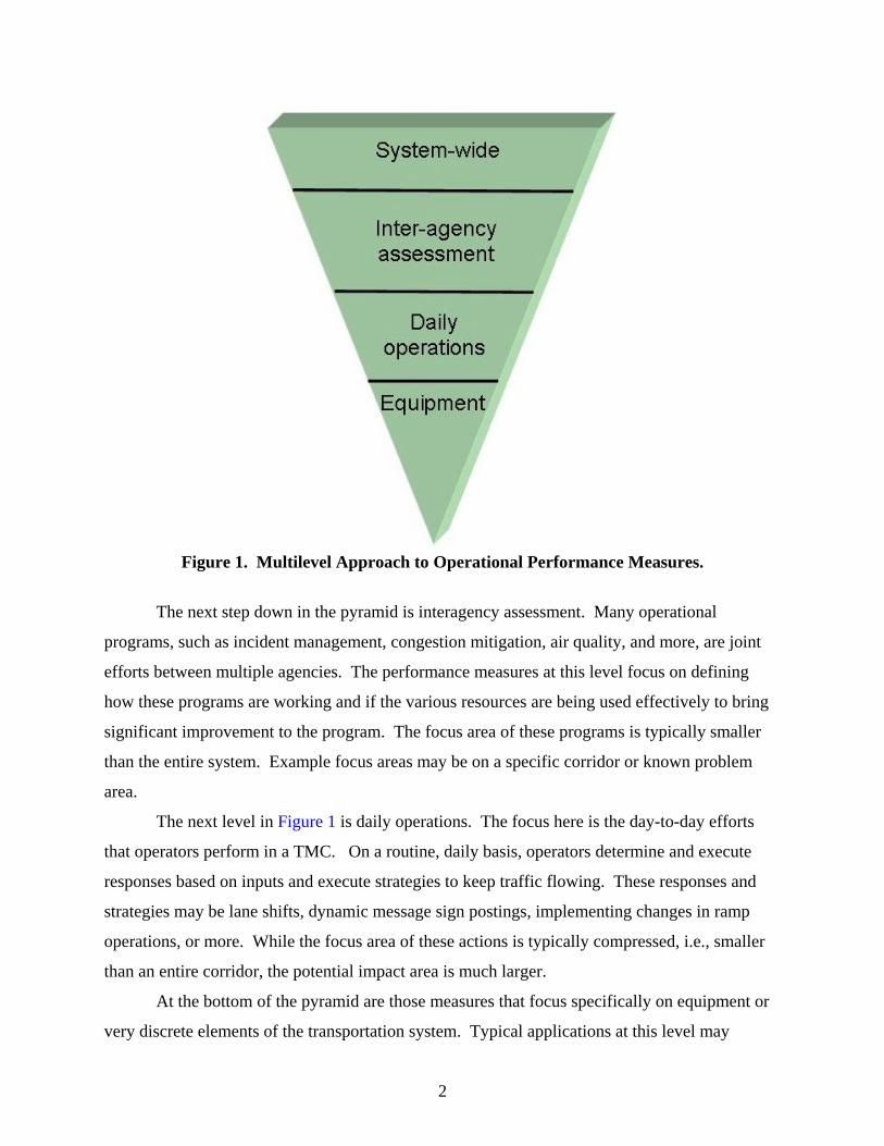
Figure 1. Multilevel Approach to Operational Performance Measures.

The next step down in the pyramid is interagency assessment. Many operational

programs, such as incident management, congestion mitigation, air quality, and more, are joint

efforts between multiple agencies. The performance measures at this level focus on defining

how these programs are working and if the various resources are being used effectively to bring

significant improvement to the program. The focus area of these programs is typically smaller

than the entire system. Example focus areas may be on a specific corridor or known problem

area.

The next level in Figure 1 is daily operations. The focus here is the day-to-day efforts

that operators perform in a TMC. On a routine, daily basis, operators determine and execute

responses based on inputs and execute strategies to keep traffic flowing. These responses and

strategies may be lane shifts, dynamic message sign postings, implementing changes in ramp

operations, or more. While the focus area of these actions is typically compressed, i.e., smaller

than an entire corridor, the potential impact area is much larger.

At the bottom of the pyramid are those measures that focus specifically on equipment or

very discrete elements of the transportation system. Typical applications at this level may

2

include items such as up-time, reliability, integrity of data, or more. Looking at these measures

should provide an overview sense of how the data collection, processing, storage, and calculation

components of performance measurement are working across the entire extent of transportation

operations.

STATE OF THE PRACTICE – OPERATIONS

Prior to the start of the research project, the general perception of the state of the practice

in traffic operations was that performance measurement for system wide assessment was

employed at some locations. Likewise, some applications were known with regard to the

equipment level and the use of measure for response time, downtime, and similar metrics. There

were no known applications of real-time operational assessment. While some TMCs may

compute a level of service (LOS) or similar measures, for use in an operator display, there were

thought to be no formalized actions taken on these values utilizing a systematic process.

In order to quantify the use of performance measurement with TxDOT, a questionnaire

was developed and administered to TMCs in Texas to categorize the use of performance

measurement across all levels shown in Figure 1. The questionnaire clearly showed that across

the state, while performance measurement is understood and appreciated for what it could

provide to transportation operations, implementation to date is minimal. This observation was

especially true in the arena of daily operations, as there were no respondents utilizing

performance measurement for that level.

One of the other findings of the questionnaire was the uncertainty surrounding which

measures could be used effectively for real-time operations. There are literally thousands of

measures that represent a particular emphasis or strategy or could potentially capture a particular

response. It is impossible, however, to implement all of the measures without creating an

incomprehensible system of data collection, storage, and analysis techniques. What is, therefore,

required is a minimal but comprehensive set of measures that can be used in daily operations to

effectively analyze actions and respond appropriately to changes.

The research team performed a literature review to determine what lists of measures have

been used external to TxDOT and if there are recommended measures for daily operations.

Several sources and lists were examined, but in the end, the list from the National Transportation

Operations Coalition (NTOC) was determined to provide the best basis for testing the

3

applicability for real-time use. The NTOC list was originally developed, with support from the

Federal Highway Administration, to define approximately 10 measures that could be commonly

agreed upon by federal, state, and local transportation officials. As stated in the NTOC final

report, these national recommendations were developed to help local traffic administrators with

the selection of performance measures and to encourage more national uniformity. The goal is

for these performance measures to be used for internal management, external communications,

and comparative measurements (3).

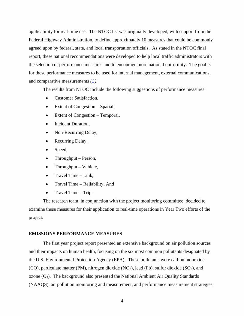
The results from NTOC include the following suggestions of performance measures:

• Customer Satisfaction,

• Extent of Congestion – Spatial,

• Extent of Congestion – Temporal,

• Incident Duration,

• Non-Recurring Delay,

• Recurring Delay,

• Speed,

• Throughput – Person,

• Throughput – Vehicle,

• Travel Time – Link,

• Travel Time – Reliability, And

• Travel Time – Trip.

The research team, in conjunction with the project monitoring committee, decided to

examine these measures for their application to real-time operations in Year Two efforts of the

project.

EMISSIONS PERFORMANCE MEASURES

The first year project report presented an extensive background on air pollution sources

and their impacts on human health, focusing on the six most common pollutants designated by

the U.S. Environmental Protection Agency (EPA). These pollutants were carbon monoxide

(CO), particulate matter (PM), nitrogen dioxide (NO2), lead (Pb), sulfur dioxide (SO2), and

ozone (O3). The background also presented the National Ambient Air Quality Standards

(NAAQS), air pollution monitoring and measurement, and performance measurement strategies

4

5

to evaluate changes in emissions from the freeway system. The conclusion from the first year

efforts was that few of the available performance measures for emissions are suited for real-time

application, and those that are, would need a significant level of monitoring stations to factor out

other influences. The report also concluded that it is questionable if the measures could achieve

the granularity required for real-time operations in a confined area.

YEAR TWO PROJECT GOALS

Operations

The guiding question behind the Year Two research work was: can the NTOC measures

be used to support real-time operations, and how can that be tested? To answer that question, the

research team, in conjunction with the project monitoring committee, decided to develop a

simulation architecture to build a performance measure display system. Using the real-time data

from the simulation would provide constantly changing data for the operator display. The

judgment of the capability of using this display to interpret real-time conditions and decide on

operational responses would be captured in a concept of operations. Project deliverable P1 is the

prototype database structure used in this simulation environment. It is contained in Chapter 3 of

this report. Project deliverable P2 is prototype displays for operator interfaces. Numerous

examples of these screens are contained in Chapter 4. Project deliverable P3, contained in

Chapter 5, is the concept of operations document for using the real-time performance measure

from the sample simulation environment.

Emissions

The conclusion of the Year One research pertaining to emissions was that there were no

factors really suited for real-time performance measurement at a cost-effective level. For that

reason, the Year Two efforts focused on providing a decision-making framework for assisting

transportation planners and operators in order to select alternative freeway performance

measures based on both qualitative measures, such as understanding, measurability, availability,

and importance, and quantitative measures, such as time, cost, accuracy, and reliability.

CHAPTER 2: REAL-TIME PERFORMANCE MEASUREMENT FOR OPERATIONS

NTOC PERFORMANCE MEASURES

The NTOC report listed 12 performance measures, as shown in Table 1. The table also

shows the basis for each performance measure and the judgment of the research team in terms of

the measure’s capability to be used in real-time. As an example, the measure of ‘Customer

Satisfaction’ is based on perception and the data requirements would be impossible to capture in

real-time. This measure is therefore not applicable for real-time usage. On the other hand, a

measure such as ‘Travel Time-Link’, which is based on speed, can be captured in real-time. It is

possible that the use of a travel time based performance measure may provide capabilities or

information to an operator that is currently not a part of any system.

Table 1. NTOC Performance Measures and Their Basis. Measure Basis Real-Time Usage Capability

Customer Satisfaction Perception No

Extent of Congestion-Spatial Speed Yes

Extent of Congestion-Temporal Speed Yes

Incident Duration Time Yes

Non-Recurring Delay Travel Time Maybe

Recurring Delay Travel Time Maybe

Speed Speed Yes

Throughput-Person Volume Yes

Throughput-Vehicle Volume Yes

Travel Time-Link Speed Yes

Travel Time-Reliability Speed Yes

Travel Time-Trip Speed Yes

It should be noted that the basis for most of the measures in Table 1 are similar, reflecting

the common data that are typically available from roadway monitoring implementations across

the nation. Many of the measures that are similar, such as the ‘throughput’ measures, differ only

by a multiplicative factor.

7

MEASURES FOR USE IN REAL-TIME PROTOTYPE TESTING

Of the 12 measures listed in the NTOC report, two were used for testing the real-time

application. This testing was a prototype experiment, and the number of measures was kept

small to balance the setup needs with the potential information gain. Also, as per the earlier

discussion, some of the measures differ only by a multiplicative factor and would not add any

knowledge to the research. The research team determined that ‘Travel Time-Link’ and ‘Extent

of Congestion-Spatial’ would be tested for real-time application. While the basis for both the

measures is speed, the extent of congestion measure examines a ratio of speeds and may yield a

different basis or interpretation than a pure link travel time.

SYSTEM ARCHITECTURE FOR REAL-TIME TESTING

As in testing measures in any prototype system, the first task was to create a generalized

system architecture that would produce the prototype displays and database called for in the

project deliverables. The method chosen to meet those needs was to create a small simulation

environment that would generate real-time data, perform the necessary calculations for creating

the NTOC performance measures, store that information in a database, and then subsequently

draw information from the database to generate operator’s displays. The main emphasis in this

architecture was to generate displays in real-time that would be representative of operator’s

displays. Figure 2 shows the overall system architecture. Each of the components will be

described in additional detail in a subsequent chapter.

Figure 2. Prototype System Architecture.

• Simulation Model – The VISSIM simulation model was used to create the

simulation environment and produce 20-second data feeds that emulate traditional

detector based roadway implementations.

• Data Manager – The data manager receives the 20-second data feeds and

manipulates the data as necessary to perform calculations of the performance

measures.

8

• Data Repository – The data repository is an Access® database that stores all of the

information necessary to feed the operator displays.

• Displays – The displays are the visual output of the specific performance

measures that can be monitored by an operator in real-time.

CALCULATION METHODOLOGY FOR TRAVEL TIME-LINK

According to the NTOC definitions, the definition of the travel time for a link is the

average time required to traverse a section of roadway in a single direction. While the NTOC

report is focused on both the planning and historical operations level, the measure can also be

examined for real-time purposes.

The travel time of the section is computed as:

)(

)()(

section

sectionsection

SpeedAverageLengthTimeTravel = Eq. 1

Where:

Length = length of the section in question

Average Speed = average of all vehicle speeds in the section during the calculation time period

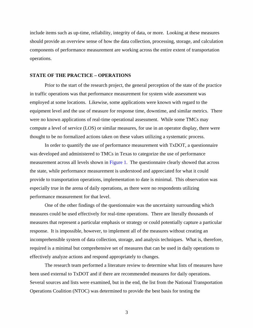
The overall steps to calculating the extent of congestion-temporal measure can be

diagrammed in a flowchart as shown in Figure 3. The methodology is very simplistic, as there

are no additional calculations beyond the computation of travel time by section. The potential

usefulness of this measure will be determined by the operator displays. Additional discussion of

these displays will be presented with the results.

9

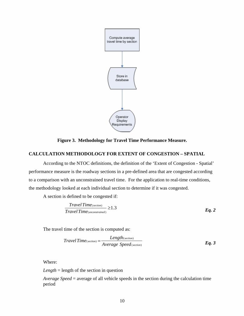
Figure 3. Methodology for Travel Time Performance Measure.

CALCULATION METHODOLOGY FOR EXTENT OF CONGESTION – SPATIAL

According to the NTOC definitions, the definition of the ‘Extent of Congestion - Spatial’

performance measure is the roadway sections in a pre-defined area that are congested according

to a comparison with an unconstrained travel time. For the application to real-time conditions,

the methodology looked at each individual section to determine if it was congested.

A section is defined to be congested if:

3.1)(

)(≥

nedunconstrai

section

TimeTravelTimeTravel Eq. 2

The travel time of the section is computed as:

)(

)()(

section

sectionsection

SpeedAverageLengthTimeTravel = Eq. 3

Where:

Length = length of the section in question

Average Speed = average of all vehicle speeds in the section during the calculation time period

10

The Travel Time(unconstrained) of the section is computed as:

)(

)()(

section

sectionednconstrainu

SpeedetargTLengthTimeTravel = Eq. 4

Where:

Target Speed = the speed that occurs when vehicles are traveling at speeds established by operations personnel as the desired speed for a given roadway during the prevailing roadway and traffic conditions

The length of the section is a static value that arises from the construction of the

simulation environment. The target speed is also a static value, but could be changed by time of

day to reflect the anticipated operating characteristics of the roadway in question. A lower target

speed might be used during the morning and evening peaks, reflecting the additional traffic that

is using the road during those time periods.

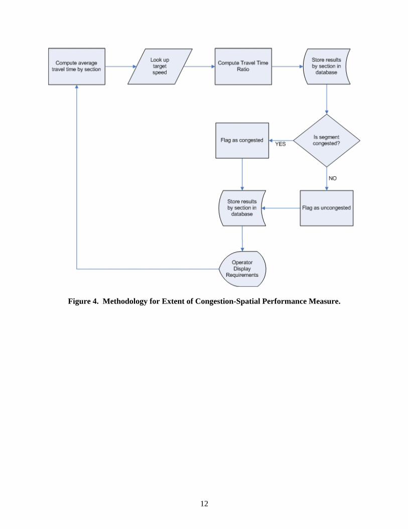
The overall steps to calculating the extent of congestion-temporal measure can be

diagrammed in a flowchart as shown in Figure 4. As is evident, this flowchart is slightly more

complex than the flowchart presented for the travel time performance measure in Figure 3. This

increase occurs because the extent of congestion performance measure incorporates a ratio of

current to unconstrained travel times by section. The target speed values must be stored in the

database along with other items such as section length, and, in addition to calculating the average

speed, the methodology must also calculate the travel time ratio. For the purposes of this

prototype, the target speeds were not changed throughout the course of the simulation time

period. The congestion flag is set according to Eq. 2 with the resulting value and flag being

stored in the database for later use in an operator display.

11

12

Figure 4. Methodology for Extent of Congestion-Spatial Performance Measure.

CHAPTER 3: COMPONENTS OF SYSTEM ARCHITECTURE

VISSIM SIMULATION MODEL

The simulation environment utilized for testing performance measures has been used

before by research performed for the Texas Department of Transportation (TxDOT) on

Project 0-4946, “Dynamic Traffic Flow Modeling for Incident Detection and Short-Term

Congestion Prediction.” A seven-mile freeway segment of Loop 1 located in the west of Austin,

Texas, from US 183 to Lake Austin Blvd was selected as a simulation test bed. Loop detectors

were placed along the simulated network to generate detector observations. The Austin detector

mapbook was consulted to ensure that detector placement in the simulated network corresponds

with actual locations. The test bed consists of a total of 69 individual inductive loop detectors on

various mainline and ramp sections. Figure 5 shows a screen capture of the simulation network.

Figure 5. VISSIM Simulation Network.

13

As with most simulation programs, VISSIM works on the concept of links and nodes.

The simulation consists of multiple links, each an individual length. Separation into the links

was determined by a number of factors, including the presence of ramps and lane additions or

drops.

In order to generate congestion during the simulation, a single-lane-block incident was

coded in the simulated network using vehicle actuated programming (VAP). This disturbance in

the normal traffic flow will illustrate the effects of changes in the traffic flow parameters on the

NTOC performance measures. The location, start time, and duration of the incident is all

specified and can be modified by the user. For the purposes of the experimental scenario, a test

incident scenario was a one-lane-blocked incident that lasted for 10 minutes near the south

terminus of the test bed. Figure 6 shows a screen capture of the simulation environment during

incident conditions.

Figure 6. VISSIM Simulation Network During Incident Conditions.

14

Figure 7 shows a screen capture of the simulation environment after the incident has

expired and traffic has cleared.

Figure 7. VISSIM Simulation Network After Incident Clearance.

DATA MANAGEMENT

There are two aspects, or programs, in use within the data management portion of the

simulation architecture.

Data Export Program

The first program retrieves the data from the simulation through the use of a custom

application developed for the 0-4946 project. The application software was developed using the

Visual Basic (VB) programming environment and integrating the VISSIM COM capability

through VB’s graphical user interface. The VISSIM COM environment is designed for users to

15

control and observe changes in traffic parameters in run-time. The software retrieves the

simulated loop detector data from VISSIM and aggregates them into a 20-second data format

similar to the Local Control Units (LCUs) in use by TxDOT. These values are output to a data

file. Each value is appended to the file so that there is a running history of all values throughout

the timeframe of the simulation.

20-Second Data From Simulation Model

Each 20-second increment contains the following data on a per lane basis:

• Time stamp – expressed in time from the beginning of the simulation, in Hours,

Minutes, and Seconds (HHMMSS);

• Detector number – the identification number of the detector to which the following

values apply;

• Volume – the total number of vehicles passing over the simulation detector within

the past 20 seconds, expressed in vehicles;

• Occupancy – the amount of time the simulation detector was occupied by a vehicle

within the past 20 seconds, expressed as a percent;

• Speed – the average of all lane specific speeds of vehicles passing over the

simulation detector within the past 20 seconds, expressed in miles per hour;

• Percent trucks – the vehicles in the 20-second vehicle stream that are reported by the

simulation as being trucks, expressed as a percentage of the total number of vehicles;

and

• Average vehicle length – the average length of all the vehicles passing over the

detector in question in the last 20 seconds, expressed in feet.

Data Feed

The data feed from the simulation is created as a comma delimited text string. Each 20-

second data string is appended to the end of the open text file during the simulation run, so that

the entire data stream of the simulation is recorded for historical purposes. Figure 8 shows an

example of the 20-second data stream.

The figure shows an initial entry of 00:55:40, representing the simulation time of

0 Hours, 55 Minutes, and 40 Seconds. Table 2 shows how the data stream can be deciphered,

16

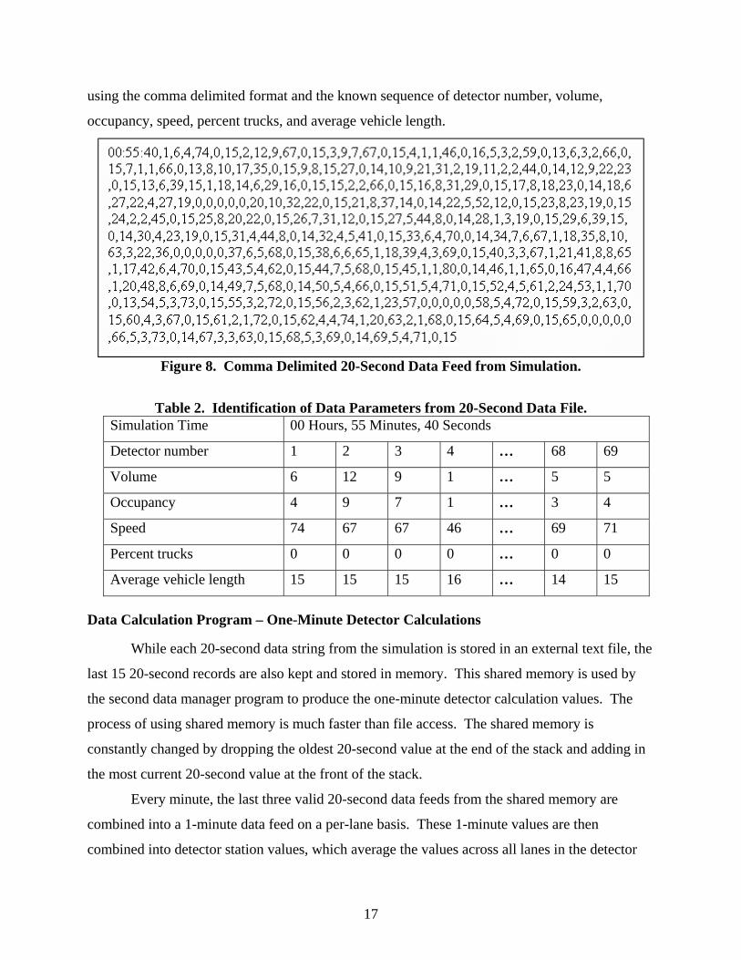
using the comma delimited format and the known sequence of detector number, volume,

occupancy, speed, percent trucks, and average vehicle length.

Figure 8. Comma Delimited 20-Second Data Feed from Simulation.

Table 2. Identification of Data Parameters from 20-Second Data File. Simulation Time 00 Hours, 55 Minutes, 40 Seconds

… Detector number 1 2 3 4 68 69

Volume 6 12 9 1 … 5 5

… Occupancy 4 9 7 1 3 4

… Speed 74 67 67 46 69 71

… Percent trucks 0 0 0 0 0 0

… Average vehicle length 15 15 15 16 14 15

Data Calculation Program – One-Minute Detector Calculations

While each 20-second data string from the simulation is stored in an external text file, the

last 15 20-second records are also kept and stored in memory. This shared memory is used by

the second data manager program to produce the one-minute detector calculation values. The

process of using shared memory is much faster than file access. The shared memory is

constantly changed by dropping the oldest 20-second value at the end of the stack and adding in

the most current 20-second value at the front of the stack.

Every minute, the last three valid 20-second data feeds from the shared memory are

combined into a 1-minute data feed on a per-lane basis. These 1-minute values are then

combined into detector station values, which average the values across all lanes in the detector

17

station. This process replicates the procedure used for roadway data implementations within

TxDOT.

The 1-minute detector station values that are calculated for use within the simulation

environment are:

• Volume – the total number of vehicles passing over the simulation detector within

the past 1 minute, expressed in vehicles;

• Average Occupancy – the average amount of time the simulation detector was

occupied by a vehicle within the past 1 minute, expressed as a percent;

• Average Speed – the average of all lane specific speeds of vehicles passing over the

simulation detector within the past 1 minute, expressed in miles per hour;

• Percent Trucks – the ratio of vehicles in the 1-minute vehicle stream that are

reported by the simulation as being trucks, expressed as a percent.

Validity Checks

The processing program for the 20-second data contains some rudimentary validity

checking to ensure that data being received are representative of real conditions. This is similar

to the validity checks that take place in the TxDOT Advanced Traffic Management System

(ATMS) using the LCU and System Control Unit (SCU). Currently, the following validity

checks are performed:

1. If Occupancy=0 and Speed=0, and Volume >0 then the data are considered invalid

and ignored.

2. If Occupancy=0 and Volume=0 and Speed is >0, then the data are considered valid

and ignored.

These basic checks essentially cover the problem of spurious data. While this event is

unlikely during a simulation run, such data issues are common in real-world implementations.

Volume

The calculation of volume is a two-step process. Step 1 is to compute the total lane

volume in the 1-minute time period as the sum of the individual volumes from the last three valid

20-second data intervals. The 1-minute lane volume calculation can be expressed as:

18

∑=

=3

1)()(

iijlane VOLUMEVOLUME Eq. 5

Where:

VOLUME lane (j) = 1-minute volume summary, per lane

VOLUME (i) = 20-second volume count, per lane

i = 20-second count index

j = lane count index.

The detector station volume average is then computed as the average of the 1-minute lane

volumes as shown in Eq. 6.

n

VOLUMEVOLUME j

jlane

kstation

∑==

3

1)(

)(Eq. 6

Where:

VOLUME station (k) = 1-minute detector station volume


j = lane count index

k = station count index

n = number of lanes.

Occupancy

The calculation of occupancy is also a two-step process and mirrors the calculations for

volume. Step 1 is to compute the average lane occupancy in the 1-minute time period using

Eq. 7.

3

3

1

)(

)(

∑== i

i

jlane

OCCUPANCYOCCUPANCY Eq. 7

Where:

OCCUPANCY lane (j) = 1-minute occupancy summary, per lane

19

OCCUPANCY (i) = 20-second occupancy count, per lane



The detector station occupancy average is then computed as the average of the 1-minute

lane occupancies as shown in Eq. 8.

n

OCCUPANCYOCCUPANCY j

jlane

kstation

∑==

3

1

)(

)(Eq. 8

Where:

OCCUPANCY station (k) = 1-minute detector station occupancy

OCCUPANCY lane (j) = 1-minute occupancy average, per lane



n = number of lanes.

Speed

The calculation of speed as performed by TxDOT field implementations is also a two-

step process but it incorporates a weighting by volume. The first step multiplies speed by

volume for each of the three, 20-second time periods in the 1-minute calculation period. This is

shown in Eq. 9 and produces a 1-minute volume-weighted speed value for each lane.

∑=

=3

1

)()()( *i

iijlane VOLUMESPEEDSPEED Eq. 9

Where:

SPEED lane (j) = 1-minute volume weighted speed, per lane

SPEED (i) = 20-second computed speed, per lane




20

The second part of the process then calculates the average weighted speed across the

entire station by Eq. 10.

∑

∑

=

== 3

1)(

3

1)(

)(

jjlane

jjlane

kstation

VOLUME

SPEEDSPEEDWEIGHTEDAVERAGE Eq. 10

Where:

AVERAGE WEIGHTED SPEED station (k) = 1-minute station average speed

SPEED lane (j) = 1-minute volume weighted speed, per lane




Percent Trucks

The calculation of percent trucks is also performed in a two-step process. Because the

simulation environment produces a value of percent trucks, the first step of the calculation is to

determine the number of trucks during the 1-minute time period as shown in Eq. 11.

∑=

=3

1

)()()( *i

iijlane VOLUMETRUCKSPERCENTTRUCKSOFNUMBER Eq. 11

Where:

NUMBER OF TRUCKS lane (j) = 1-minute number of trucks, per lane

PERCENT TRUCKS (i) = 20-second percent trucks value, per lane




The calculation of the percentage of trucks across the entire detector station is then

performed using Eq. 12, which divides the sum of the 1-minute truck values across all lanes by

21

the total volume across all lanes. The detector station percent trucks calculation is performed in

this manner to account for uneven volumes during the 20-second time periods, which would

skew the final percent trucks number if a simple average were taken.

∑

∑

=

== 3

1)(

3

1)(

)(

jjlane

jjlane

kstation

VOLUME

TRUCKSOFNUMBERTRUCKSPERCENT Eq. 12

Where:

PERCENT TRUCKS station (k) = 1-minute station average speed

NUMBER OF TRUCKS lane (j) = 1-minute sum of the number of trucks, per lane




DATABASE

Perhaps one of the most critical aspects of testing a real-time performance measurement

application to operations is defining a storage medium to use when performing calculations

pertaining to the various measures. While using shared memory for the most recent fifteen

records of 20-second data works well, the use of shared memory is not practical for storing

calculation results over the course of the entire simulation. For both that reason and the

additional aspect of keeping an archive of the data produced by the various calculations, the use

of an external storage mechanism is an integral component of the system architecture for the

prototype performance measures application.

The research team developed the prototype database by looking not only at the

calculations required for the two measures tested in the prototype, but by examining a number of

calculations required for the NTOC measures that have potential for real-time application. As

stated previously, some NTOC measures such as ‘Customer Satisfaction’ are not suitable for

real-time use by the nature of the required data collection. In addition to the measures for

NTOC, the research team theorized two additional measures, using delay as a substitute for

travel time.

22

23

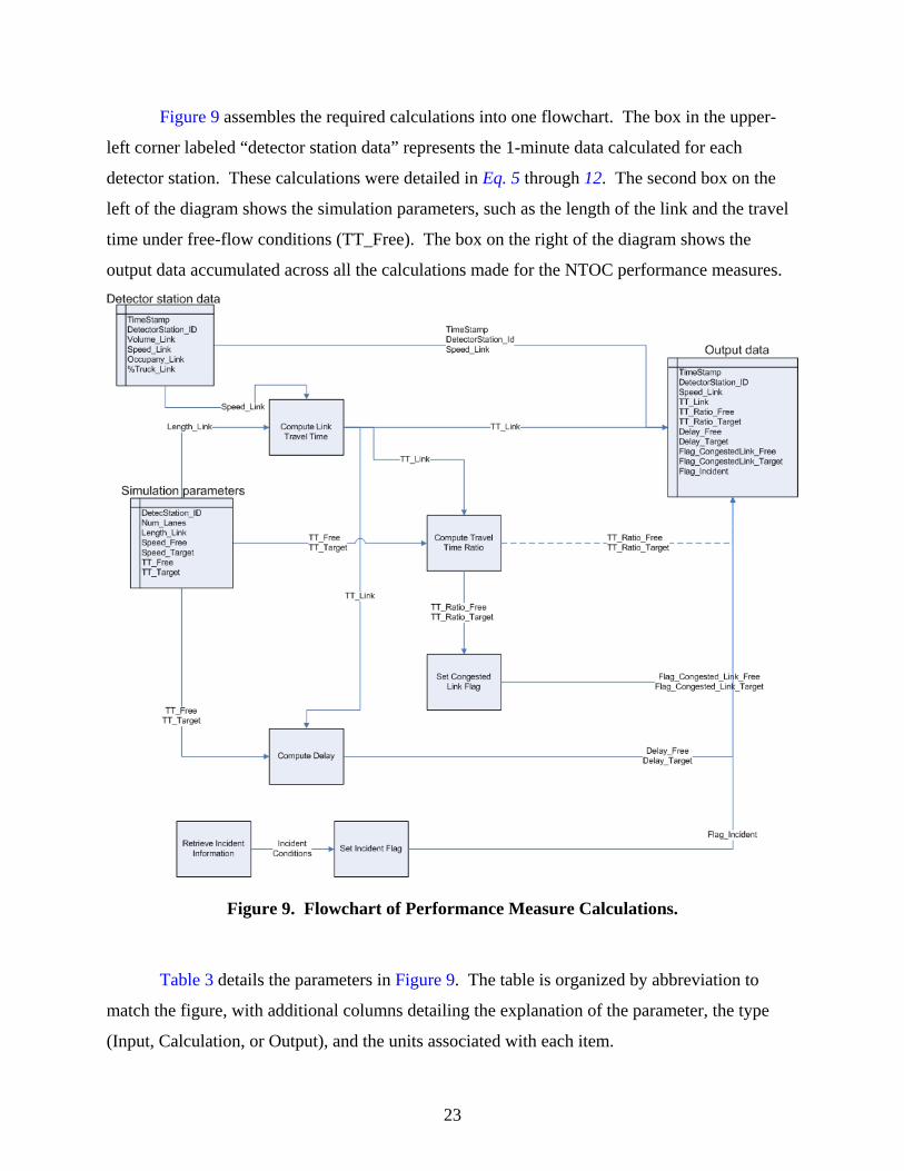
Figure 9 assembles the required calculations into one flowchart. The box in the upper-

left corner labeled “detector station data” represents the 1-minute data calculated for each

detector station. These calculations were detailed in Eq. 5 through 12. The second box on the

left of the diagram shows the simulation parameters, such as the length of the link and the travel

time under free-flow conditions (TT_Free). The box on the right of the diagram shows the

output data accumulated across all the calculations made for the NTOC performance measures.

Figure 9. Flowchart of Performance Measure Calculations.

Table 3 details the parameters in Figure 9. The table is organized by abbreviation to

match the figure, with additional columns detailing the explanation of the parameter, the type

(Input, Calculation, or Output), and the units associated with each item.

T

able

3.

Para

met

ers U

sed

in P

erfo

rman

ce M

easu

rem

ent C

alcu

latio

ns.

24

Abb

revi

atio

n Ex

plan

atio

n Ty

pe

Uni

ts

Tim

eSta

mp

Tim

e st

amp

sinc

e be

ginn

ing

of si

mul

atio

n In

put/O

utpu

t Ti

me

(HH

MM

SS)

Det

ecto

rSta

tion_

ID

Uni

que

iden

tific

atio

n nu

mbe

r of d

etec

tor s

tatio

n In

put/O

utpu

t U

nitle

ss

Num

_Lan

es

The

num

ber o

f lan

es in

the

dete

ctor

stat

ion

Inpu

t N

umbe

r of l

anes

Le

ngth

_Lin

k Th

e le

ngth

of e

ach

link

in th

e si

mul

atio

n In

put

Feet

Sp

eed_

Free

U

ncon

stra

ined

(fre

e flo

w) s

peed

on

the

link

In

put

Mile

s per

hou

r Sp

eed_

Targ

et

Ope

rato

r des

ired

spee

d on

the

link

Inpu

t M

iles p

er h

our

TT_F

ree

Unc

onst

rain

ed (f

ree

flow

) tra

vel t

ime

on th

e lin

k

Inpu

t/Cal

cula

ted

Min

utes

TT

_Tar

get

Ope

rato

r des

ired

trave

l tim

e on

the

link

Inpu

t/Cal

cula

ted

Min

utes

V

olum

e_Li

nk

Cal

cula

ted

1-m

inut

e de

tect

or st

atio

n vo

lum

e

Cal

cula

ted

Veh

icle

s per

hou

r Sp

eed_

Link

C

alcu

late

d 1-

min

ute

dete

ctor

stat

ion

spee

d C

alcu

late

d/O

utpu

tM

iles p

er h

our

Occ

upan

cy_L

ink

Cal

cula

ted

1-m

inut

e de

tect

or st

atio

n oc

cupa

ncy

C

alcu

late

d U

nitle

ss

%Tr

uck_

Link

C

alcu

late

d 1-

min

ute

dete

ctor

stat

ion

perc

ent t

ruck

s C

alcu

late

d U

nitle

ss

TT_L

ink

Cal

cula

ted

trave

l tim

e on

link

C

alcu

late

d/O

utpu

tM

inut

es

TT_R

atio

_Fre

e C

alcu

late

d tra

vel t

ime

ratio

on

link

(cur

rent

to d

esire

d fr

ee)

Cal

cula

ted/

Out

put

Uni

tless

TT

_Rat

io_T

arge

t C

alcu

late

d tra

vel t

ime

ratio

on

link

(cur

rent

to d

esire

d ta

rget

) C

alcu

late

d/O

utpu

tU

nitle

ss

Flag

_Con

gest

ed_L

ink_

Free

C

onge

stio

n fla

g fo

r lin

ks c

alcu

late

d on

bas

is o

f TT_

Free

C

alcu

late

d/O

utpu

tU

nitle

ss

Flag

_Con

gest

ed_L

ink_

Targ

et

Con

gest

ion

flag

for l

inks

cal

cula

ted

on b

asis

of T

T_Ta

rget

C

alcu

late

d/O

utpu

tU

nitle

ss

Del

ay_F

ree

Cal

cula

ted

link

dela

y ba

sed

on fr

ee fl

ow sp

eed

Cal

cula

ted/

Out

put

Min

utes

D

elay

_Tar

get

Cal

cula

ted

link

dela

y ba

sed

on ta

rget

spee

d C

alcu

late

d/O

utpu

tM

inut

es

Flag

_Inc

iden

t C

onge

stio

n fla

g fo

r pre

senc

e of

inci

dent

C

alcu

late

d/O

utpu

tU

nitle

ss

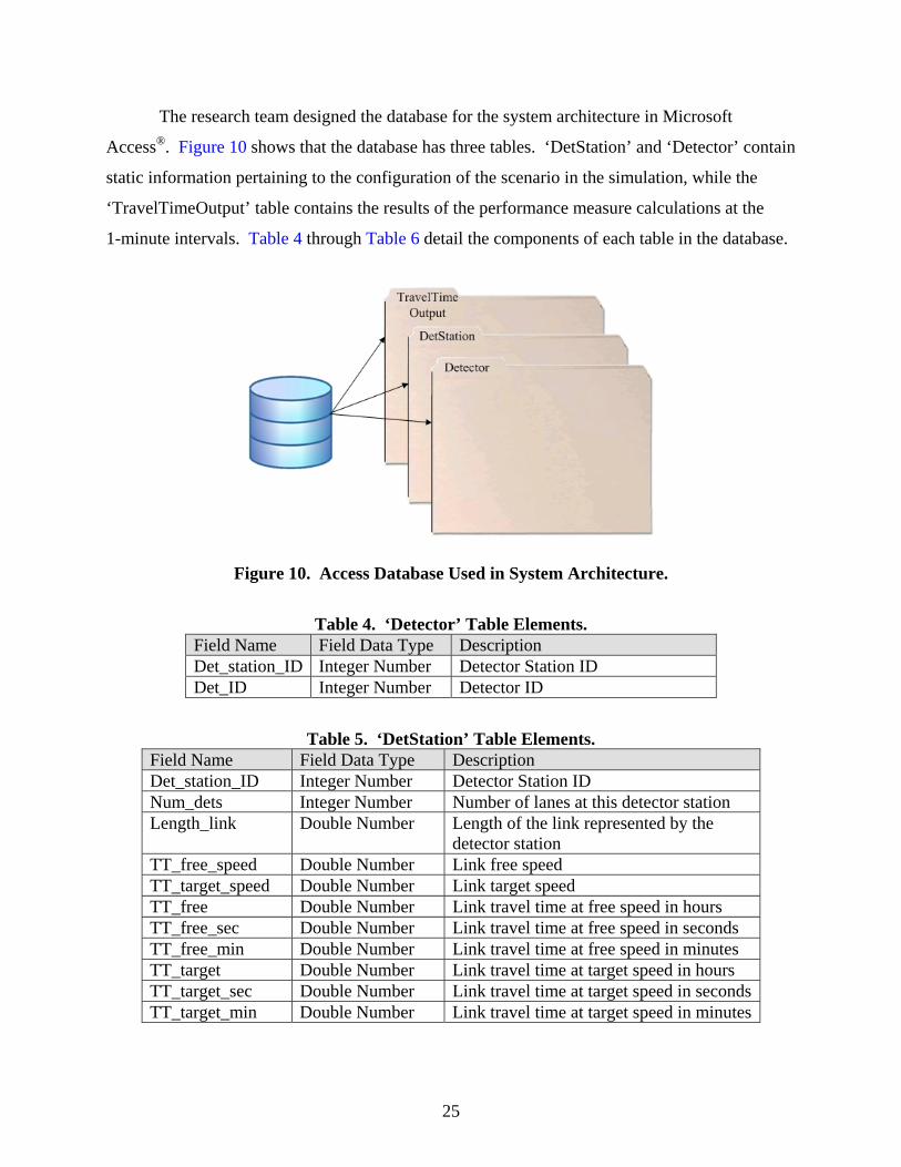
The research team designed the database for the system architecture in Microsoft

Access®. Figure 10 shows that the database has three tables. ‘DetStation’ and ‘Detector’ contain

static information pertaining to the configuration of the scenario in the simulation, while the

‘TravelTimeOutput’ table contains the results of the performance measure calculations at the

1-minute intervals. Table 4 through Table 6 detail the components of each table in the database.

Figure 10. Access Database Used in System Architecture.

Table 4. ‘Detector’ Table Elements. Field Name Field Data Type Description Det_station_ID Integer Number Detector Station ID Det_ID Integer Number Detector ID

Table 5. ‘DetStation’ Table Elements. Field Name Field Data Type Description Det_station_ID Integer Number Detector Station ID Num_dets Integer Number Number of lanes at this detector station Length_link Double Number Length of the link represented by the

detector station TT_free_speed Double Number Link free speed TT_target_speed Double Number Link target speed TT_free Double Number Link travel time at free speed in hours TT_free_sec Double Number Link travel time at free speed in seconds TT_free_min Double Number Link travel time at free speed in minutes TT_target Double Number Link travel time at target speed in hours TT_target_sec Double Number Link travel time at target speed in secondsTT_target_min Double Number Link travel time at target speed in minutes

25

26

Table 6. ‘TravelTimeOutput’ Table Elements. Field Name Field Data Type Description Det_station_ID Integer Number Detector Station ID Length_link Double Number Length of the link represented by the

detector station Time_stamp Text – 11

characters The 20-second time interval. Time stamp starts at 00:00:00 (HH:MM:SS)

Speed_link Integer Number Current 20-second average speed of link TT_link Double Number Link travel time at current 20-second

speed in hours TT_link_sec Double Number Link travel time at current 20-second

speed in seconds TT_link_min Double Number Link travel time at current 20-second

speed in minutes TT_ratio_free Double Number Ratio of the link travel time at current

speed to link travel time at free speed TT_ratio_target Double Number Ratio of the link travel time at current

speed to link travel time at target speed Delay_free Double Number Difference between link travel time at

current speed and link travel time at free speed

Delay_target Double Number Difference between link travel time at current speed and link travel time at target speed

Congested_free_link_flag Yes/No If TT_ratio_free > 1.3 link is congested

Congested_target_link_flag Yes/No If TT_ratio_target > 1.3 link is congested

Incident_flag Yes/No

CHAPTER 4: OPERATOR DISPLAYS

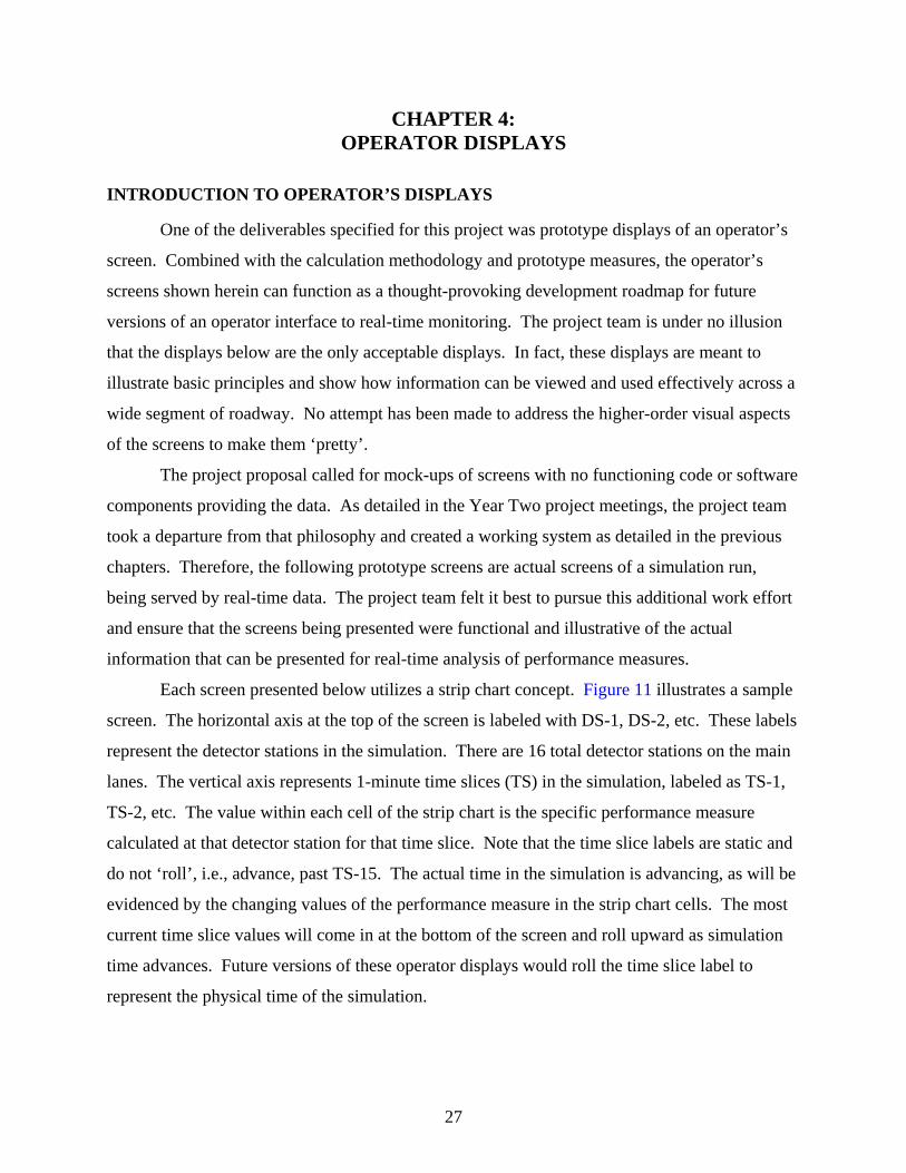
INTRODUCTION TO OPERATOR’S DISPLAYS

One of the deliverables specified for this project was prototype displays of an operator’s

screen. Combined with the calculation methodology and prototype measures, the operator’s

screens shown herein can function as a thought-provoking development roadmap for future

versions of an operator interface to real-time monitoring. The project team is under no illusion

that the displays below are the only acceptable displays. In fact, these displays are meant to

illustrate basic principles and show how information can be viewed and used effectively across a

wide segment of roadway. No attempt has been made to address the higher-order visual aspects

of the screens to make them ‘pretty’.

The project proposal called for mock-ups of screens with no functioning code or software

components providing the data. As detailed in the Year Two project meetings, the project team

took a departure from that philosophy and created a working system as detailed in the previous

chapters. Therefore, the following prototype screens are actual screens of a simulation run,

being served by real-time data. The project team felt it best to pursue this additional work effort

and ensure that the screens being presented were functional and illustrative of the actual

information that can be presented for real-time analysis of performance measures.

Each screen presented below utilizes a strip chart concept. Figure 11 illustrates a sample

screen. The horizontal axis at the top of the screen is labeled with DS-1, DS-2, etc. These labels

represent the detector stations in the simulation. There are 16 total detector stations on the main

lanes. The vertical axis represents 1-minute time slices (TS) in the simulation, labeled as TS-1,

TS-2, etc. The value within each cell of the strip chart is the specific performance measure

calculated at that detector station for that time slice. Note that the time slice labels are static and

do not ‘roll’, i.e., advance, past TS-15. The actual time in the simulation is advancing, as will be

evidenced by the changing values of the performance measure in the strip chart cells. The most

current time slice values will come in at the bottom of the screen and roll upward as simulation

time advances. Future versions of these operator displays would roll the time slice label to

represent the physical time of the simulation.

27

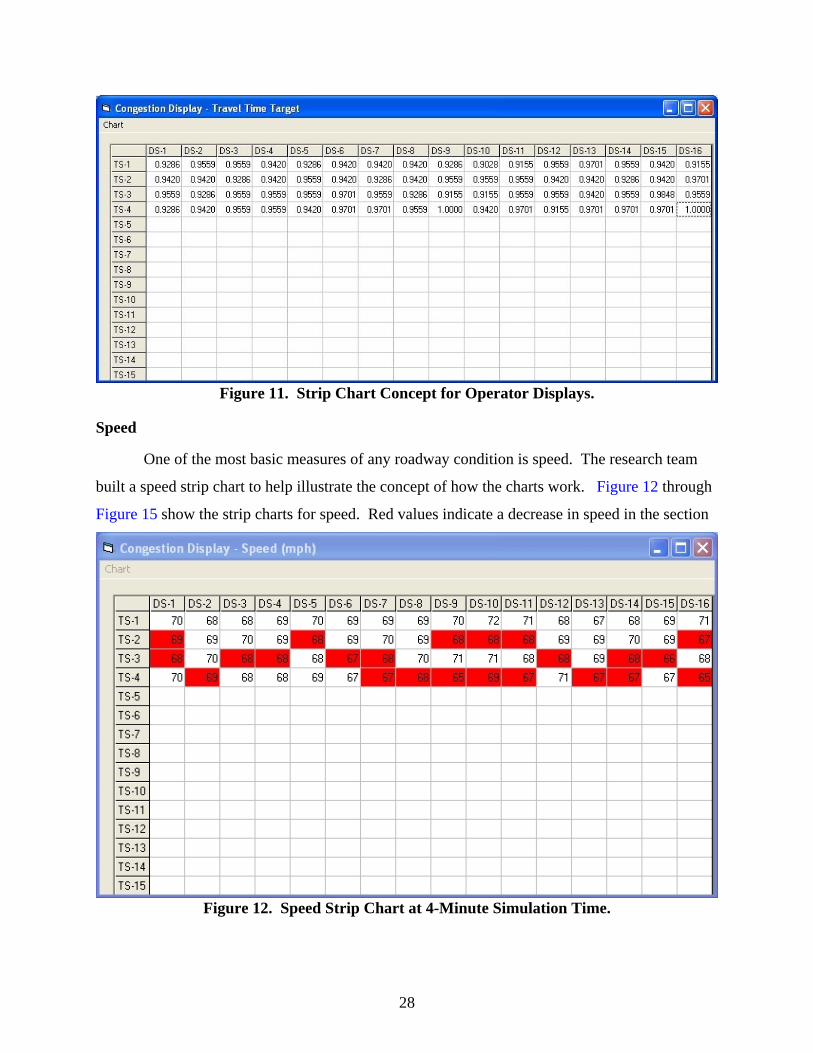
Figure 11. Strip Chart Concept for Operator Displays.

Speed

One of the most basic measures of any roadway condition is speed. The research team

built a speed strip chart to help illustrate the concept of how the charts work. Figure 12 through

Figure 15 show the strip charts for speed. Red values indicate a decrease in speed in the section

Figure 12. Speed Strip Chart at 4-Minute Simulation Time.

28



29


from the previous time slice. By itself, the indications of change in the speed parameter mean

very little as they vary continuously in real-time. The highlighting, however, illustrates how the

charts work. In practical application, the highlight would likely be restricted from showing

unless the speed in a particular section dropped below a target value, such as the “Speed_Target”

value from Table 3. This would be an operator-adjusted value.

Travel Time-Link

Travel time on a link is one of the measures in the NTOC list that was examined for real-

time application. Figure 16 through Figure 18 show the travel time strip charts at a 4-, 15-, and

30-minute simulation time. (Recall that the time slice headings on the vertical axis do not

currently roll to reflect simulation time. A quick visual examination will show that the values in

the individual cells in the figures are different.)

The perceived usefulness of real-time monitoring of travel time on a link is mixed. On

one hand, the strip charts provide an immediate and up-to-date assessment of roadway conditions

that are important to a traveler. These strip charts prove that the concept of monitoring the

NTOC measure in real-time is indeed possible.

30

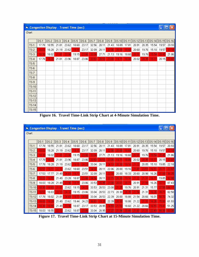
Figure 16. Travel Time-Link Strip Chart at 4-Minute Simulation Time.


31


However, the concern with travel time monitoring is the same as with speed. Even a

slight change in travel time introduces a flag to color the cell red. For a practical application, the

alert should only come on when the travel time drops below a specified value, such as the

‘TT_Target’ value in Table 3. Ideally, this parameter would be specified by time of day and by

detector station, and would act as a yardstick to measure against the current travel time across the

detector station.

Extent of Congestion – Spatial

The research team felt that the NTOC measures developed to examine the extent of

congestion also held significant potential to identify when and where an incident or traffic

disruption starts, as well as showing the affect across the rest of the system. Because the

measure utilizes a ratio of current travel time to a desired travel time, instead of an absolute

value, the measure should be less susceptible to slight changes and yet still be reactive to

significant changes in the conditions. The strip charts illustrated in Figure 19 through Figure 25

use the ‘TT_Target’ as the denominator in the calculation of the ratio.

32

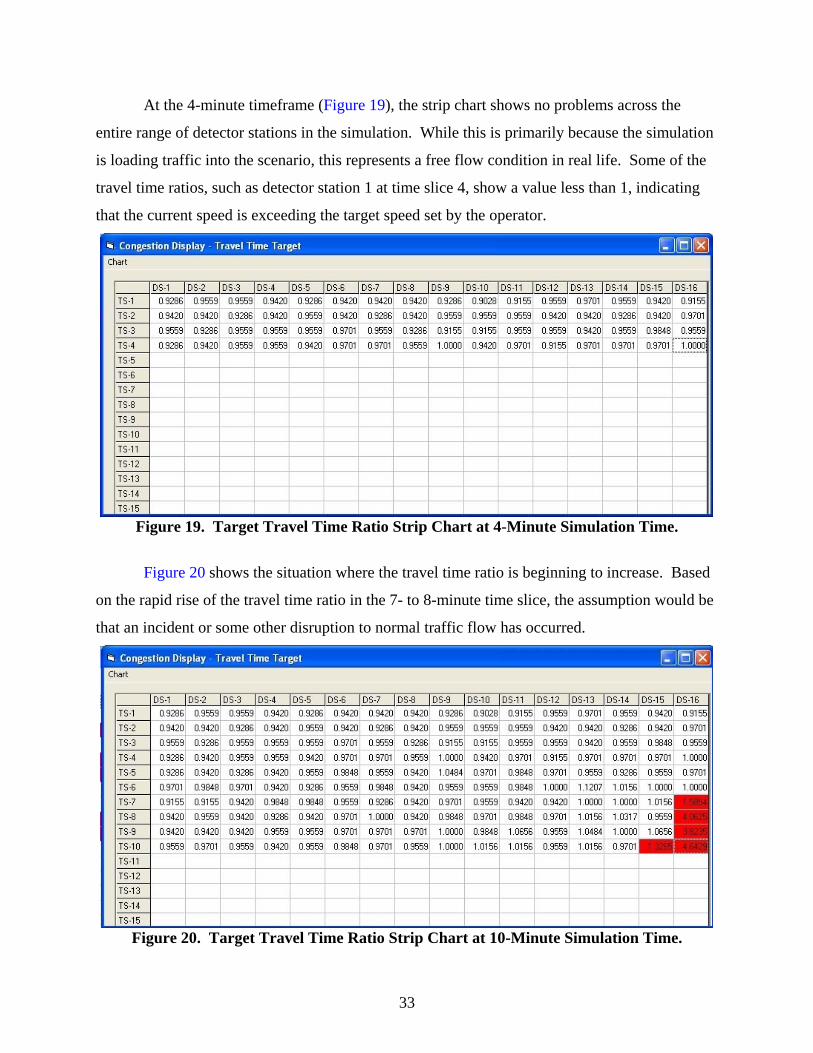
At the 4-minute timeframe (Figure 19), the strip chart shows no problems across the

entire range of detector stations in the simulation. While this is primarily because the simulation

is loading traffic into the scenario, this represents a free flow condition in real life. Some of the

travel time ratios, such as detector station 1 at time slice 4, show a value less than 1, indicating

that the current speed is exceeding the target speed set by the operator.

Figure 19. Target Travel Time Ratio Strip Chart at 4-Minute Simulation Time.

Figure 20 shows the situation where the travel time ratio is beginning to increase. Based

on the rapid rise of the travel time ratio in the 7- to 8-minute time slice, the assumption would be

that an incident or some other disruption to normal traffic flow has occurred.


33

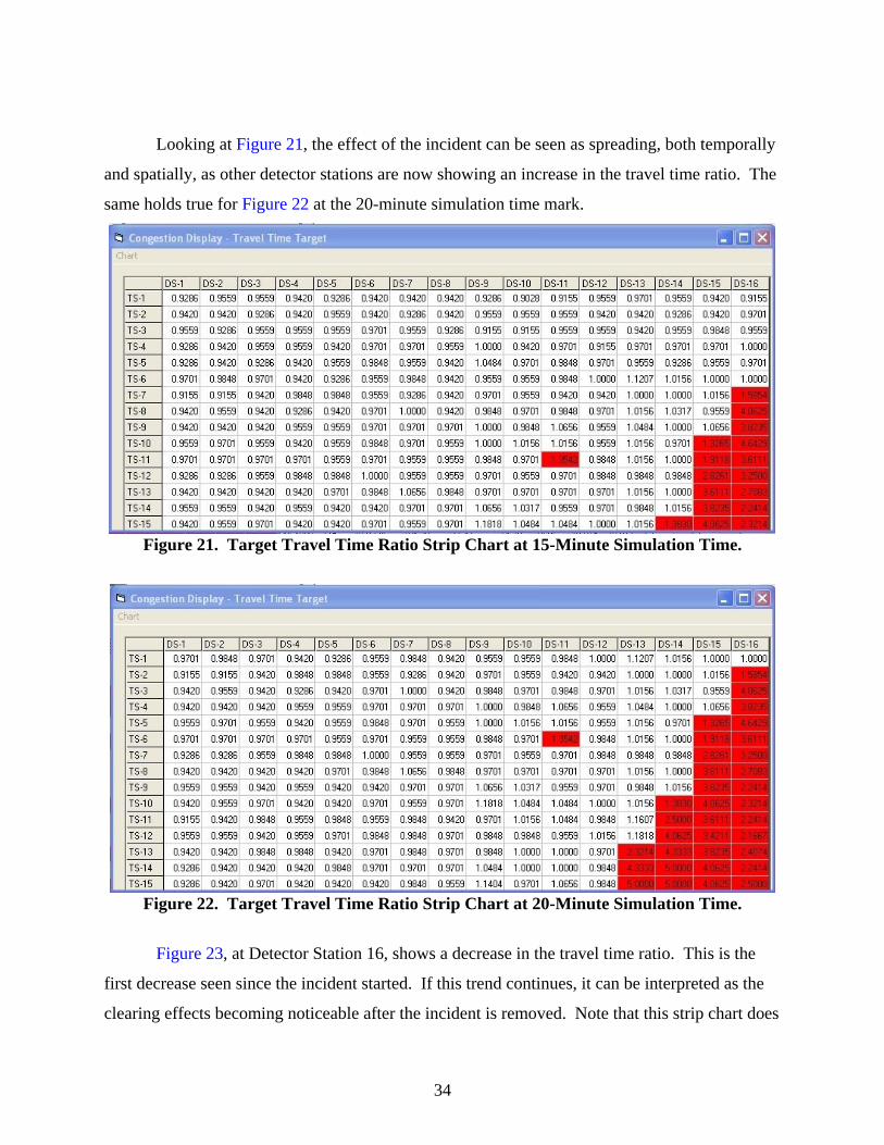
Looking at Figure 21, the effect of the incident can be seen as spreading, both temporally

and spatially, as other detector stations are now showing an increase in the travel time ratio. The

same holds true for Figure 22 at the 20-minute simulation time mark.



Figure 23, at Detector Station 16, shows a decrease in the travel time ratio. This is the

first decrease seen since the incident started. If this trend continues, it can be interpreted as the

clearing effects becoming noticeable after the incident is removed. Note that this strip chart does

34

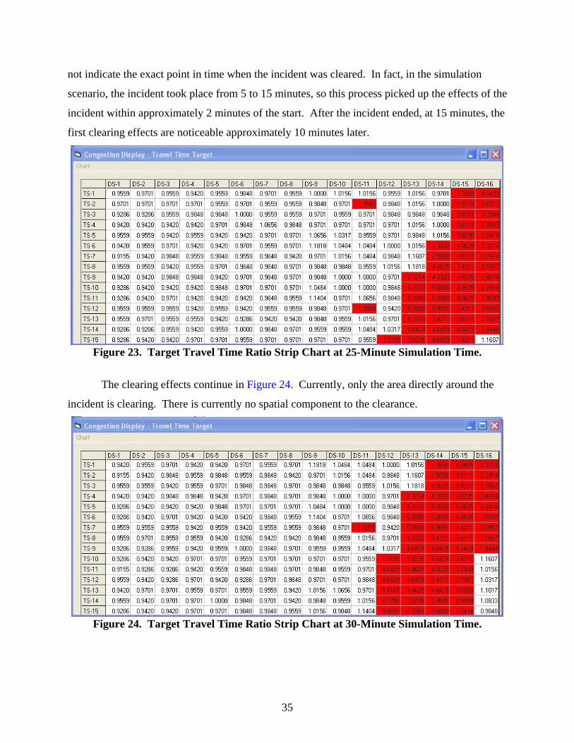
not indicate the exact point in time when the incident was cleared. In fact, in the simulation

scenario, the incident took place from 5 to 15 minutes, so this process picked up the effects of the

incident within approximately 2 minutes of the start. After the incident ended, at 15 minutes, the

first clearing effects are noticeable approximately 10 minutes later.


The clearing effects continue in Figure 24. Currently, only the area directly around the

incident is clearing. There is currently no spatial component to the clearance.


35

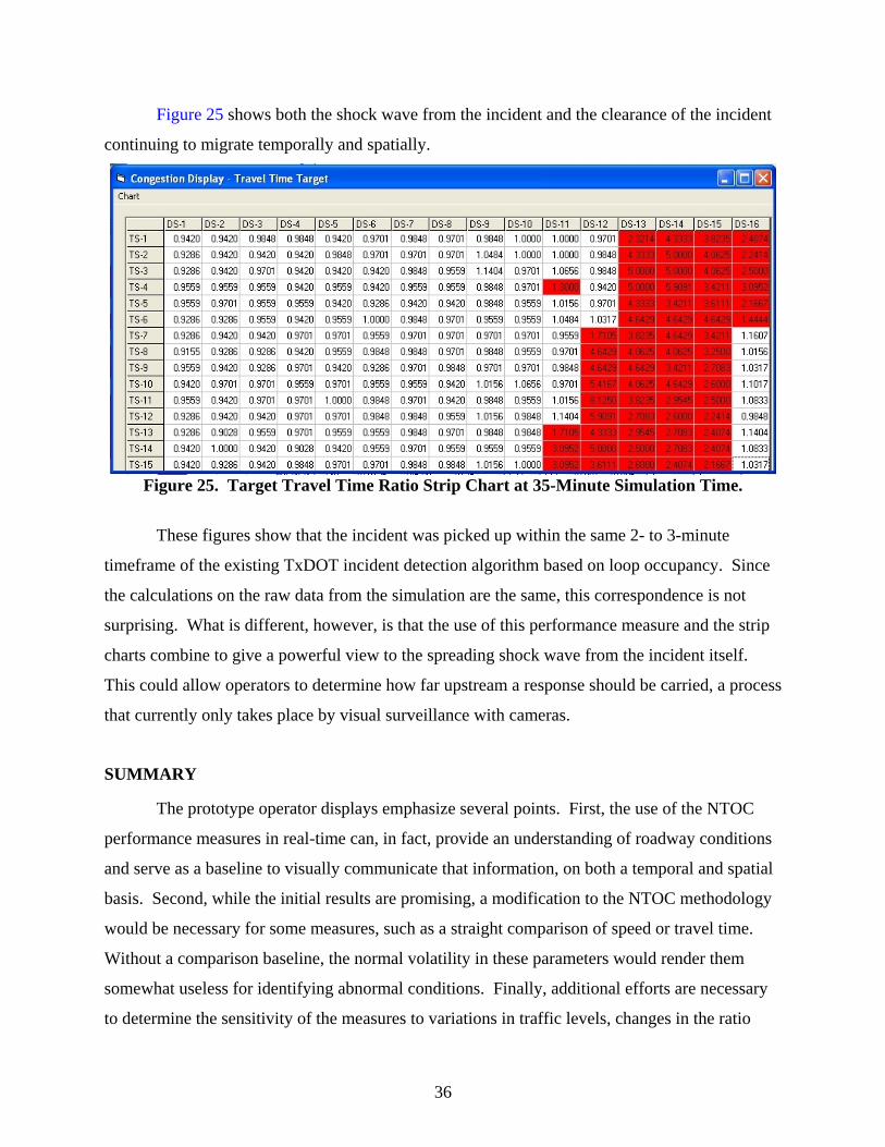
Figure 25 shows both the shock wave from the incident and the clearance of the incident

continuing to migrate temporally and spatially.


These figures show that the incident was picked up within the same 2- to 3-minute

timeframe of the existing TxDOT incident detection algorithm based on loop occupancy. Since

the calculations on the raw data from the simulation are the same, this correspondence is not

surprising. What is different, however, is that the use of this performance measure and the strip

charts combine to give a powerful view to the spreading shock wave from the incident itself.

This could allow operators to determine how far upstream a response should be carried, a process

that currently only takes place by visual surveillance with cameras.

SUMMARY

The prototype operator displays emphasize several points. First, the use of the NTOC

performance measures in real-time can, in fact, provide an understanding of roadway conditions

and serve as a baseline to visually communicate that information, on both a temporal and spatial

basis. Second, while the initial results are promising, a modification to the NTOC methodology

would be necessary for some measures, such as a straight comparison of speed or travel time.

Without a comparison baseline, the normal volatility in these parameters would render them

somewhat useless for identifying abnormal conditions. Finally, additional efforts are necessary

to determine the sensitivity of the measures to variations in traffic levels, changes in the ratio

36

37

value used, etc. Additionally, a determination of the sensitivity of the travel time ratio

performance measure should be made if the target travel time values change by time of day, as

determined by an operator.

CHAPTER 5: CONCEPT OF OPERATIONS

BACKGROUND

A comprehensive Concept of Operations (COO) document typically addresses the Who,

What, When, Where, Why, and How aspects of a system. The COO is intended to reach a wide

audience. Generally, the level of detail is balanced between being general enough for

stakeholders external to the implementation, with enough information to provide the basis for

specific requirements for system implementation. The typical components of a COO might

include:

• scope,

• references,

• operational description,

• operational needs,

• system overview,

• support environment, and

• operational scenarios.

While the above components are typical, it should be understood that the COO is not a

one-size-fits-all document. COOs and the elements they contain are expected to be tailored to

the unique aspects of the system under discussion.

COO FOR REAL-TIME PERFORMANCE MEASURE: ‘EXTENT OF CONGESTION-SPATIAL’

Within the research of this project, speed, travel time, and the spatial extent of congestion

were tested as potential performance measures for real-time usage. Speed and travel time may

show future usage, although a real-time implementation would have to move beyond the NTOC

definitions and incorporate some type of comparison to historical, or set values, in order to

remove the alerts that result from the normal volatility in traffic. The spatial extent of

congestion, however, showed significant potential for real-time usage direct from the NTOC

recommendations. A COO will be developed for the usage of this performance measure.

39

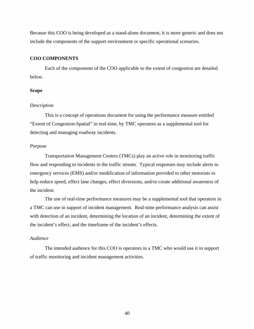
Because this COO is being developed as a stand-alone document, it is more generic and does not

include the components of the support environment or specific operational scenarios.

COO COMPONENTS

Each of the components of the COO applicable to the extent of congestion are detailed

below.

Scope

Description

This is a concept of operations document for using the performance measure entitled

“Extent of Congestion-Spatial” in real-time, by TMC operators as a supplemental tool for

detecting and managing roadway incidents.

Purpose

Transportation Management Centers (TMCs) play an active role in monitoring traffic

flow and responding to incidents in the traffic stream. Typical responses may include alerts to

emergency services (EMS) and/or modification of information provided to other motorists to

help reduce speed, effect lane changes, effect diversions, and/or create additional awareness of

the incident.

The use of real-time performance measures may be a supplemental tool that operators in

a TMC can use in support of incident management. Real-time performance analysis can assist

with detection of an incident, determining the location of an incident, determining the extent of

the incident’s effect, and the timeframe of the incident’s effects.

Audience

The intended audience for this COO is operators in a TMC who would use it in support

of traffic monitoring and incident management activities.

40

References

The reference for the ‘Extent of Congestion-Spatial’ performance measure is the

“National Transportation Operations Coalition (NTOC) Performance Measurement Initiative.

Final Report.”(3).

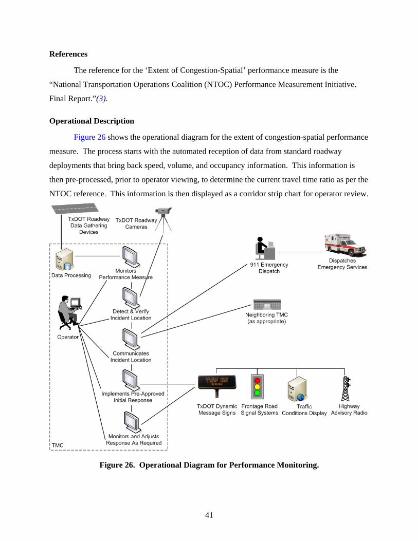
Operational Description

Figure 26 shows the operational diagram for the extent of congestion-spatial performance

measure. The process starts with the automated reception of data from standard roadway

deployments that bring back speed, volume, and occupancy information. This information is

then pre-processed, prior to operator viewing, to determine the current travel time ratio as per the

NTOC reference. This information is then displayed as a corridor strip chart for operator review.

Figure 26. Operational Diagram for Performance Monitoring.

41

When an incident is presumed (as an example, refer to Figure 19 through Figure 25), the

operator would typically verify the incident with appropriate surveillance cameras. The primary

action following confirmation would be to alert emergency services, if necessary. A

communication may also be sent to neighboring TMCs, depending on the location, type, and

expected duration of the incident.

Following notification, the TMC operator would assess what actions and/or information

can and should be presented to the traveling public pertaining to the incident. Options for

actions may include alerting motorists via dynamic message signs, highway advisory radio, the

traffic conditions display, and media. The operator may also alter ramp and or frontage road

signal operations, as appropriate, to allow for better diversion patterns. Throughout the duration

of the incident, the operator will continue to monitor and adjust the traffic response plan, as

appropriate.

Operational Needs

Incorporation of real-time performance monitoring using the ‘Extent of Congestion-

Spatial’ measure, supplements the available information for effectively managing the roadway,

particularly during incidents. Implemented as a corridor view, the performance measure

provides a comprehensive, data-driven, data-responsive, real-time assessment of the incident’s

impacts beyond the visual scope of looking at surveillance cameras. To implement this measure,

the following general needs are noted:

• pre-processing capability for roadway data,

• information processing capability for processed data,

• ability to access and control roadway surveillance capabilities,

• real-time information updates to TMC operators,

• ability to communicate incident location and associated information to emergency

services and/or other TMCs, and

• ability to control roadway infrastructure.

42

System Overview

System Scope

The scope of the real-time performance measurement system can be system wide,

although the view into the data should be performed at a corridor level.

System Users

The users of this real-time performance measuring capability are TMC operators.

Interfaces

Externally, the system must interface to the data communications feed from roadway

sensors. Internally, the pre-processing component must interface to the information displays

viewable by TMC operators.

Capabilities

The system should have the capability to display the ‘Extent of Congestion-Spatial’

performance measure in real-time on a corridor basis. Expected minimal output is a strip chart

format with spatial measurements on the horizontal axis and temporal measurements on the

vertical axis. Temporal components should roll vertically, with at least a 15-minute display

being visible at all times. The strip chart interface should place the current value of the

performance measure within each cell (intersection of time and spatial component). Cells should

be color coded for a visual alert if the value of the previous time slice within the same spatial

component is less than the value of the current time slice. Example strip charts can be seen in

Figure 19 through Figure 25.

Completed COO

The complete COO is shown in Table 7.

43

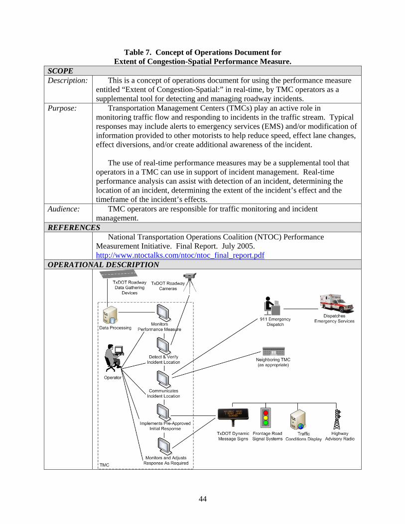
Table 7. Concept of Operations Document for Extent of Congestion-Spatial Performance Measure.

SCOPE Description: This is a concept of operations document for using the performance measure

entitled “Extent of Congestion-Spatial:” in real-time, by TMC operators as a supplemental tool for detecting and managing roadway incidents.

Purpose: Transportation Management Centers (TMCs) play an active role in monitoring traffic flow and responding to incidents in the traffic stream. Typical responses may include alerts to emergency services (EMS) and/or modification of information provided to other motorists to help reduce speed, effect lane changes, effect diversions, and/or create additional awareness of the incident.

The use of real-time performance measures may be a supplemental tool that

operators in a TMC can use in support of incident management. Real-time performance analysis can assist with detection of an incident, determining the location of an incident, determining the extent of the incident’s effect and the timeframe of the incident’s effects.

Audience: TMC operators are responsible for traffic monitoring and incident management.

REFERENCES National Transportation Operations Coalition (NTOC) Performance

Measurement Initiative. Final Report. July 2005. http://www.ntoctalks.com/ntoc/ntoc_final_report.pdf

OPERATIONAL DESCRIPTION

44

http://www.ntoctalks.com/ntoc/ntoc_final_report.pdf

Table 7. Concept of Operations Document for Extent of Congestion-Spatial Performance Measure (continued).

OPERATIONAL DESCRIPTION (continued) The operational diagram shows that the process starts with the automated

reception of data from standard roadway deployments that bring back speed, volume, and occupancy information. This information is then pre-processed, prior to operator viewing, to determine the current travel time ratio as per the NTOC reference. This information is then displayed as a corridor strip chart for operator review.

When an incident is presumed (as an example refer to Figure 19 through

Figure 25), the operator would typically verify the incident with appropriate surveillance cameras. The primary action following confirmation would be to alert emergency services, if necessary. A communication may also be sent to neighboring TMCs, depending on the location, type, and expected duration of the incident.

Following notification, the TMC operator would assess what actions and/or

information can and should be presented to the traveling public pertaining to the incident. Options for actions may include alerting motorists via dynamic message signs, highway advisory radio, the traffic conditions display, and media. The operator may also alter ramp and/or frontage road signal operations, as appropriate, to allow for better diversion patterns. Throughout the duration of the incident, the operator will continue to monitor and adjust the traffic response plan, as appropriate.

OPERATIONAL NEEDS Incorporation of real-time performance monitoring using the ‘Extent of

Congestion-Spatial’ measure, supplements the available information for effectively managing the roadway, particularly during incidents. Implemented as a corridor view, the performance measure provides a comprehensive, data-driven, data-responsive, real-time assessment of the incident’s impacts beyond the visual scope of looking at surveillance cameras. To implement this measure, the following general needs are noted:

• pre-processing capability for roadway data, • information processing capability for processed data, • ability to access and control roadway surveillance capabilities, • real-time information updates to TMC operators, • ability to communicate incident location and associated information to

emergency services and/or other TMCs, and • ability to control roadway infrastructure.

SYSTEM OVERVIEW Scope The scope of the real-time performance measurement system can be system

wide, although the view into the data should be performed at a corridor level. Users The users of this real-time performance measuring capability are TMC

operators.

45

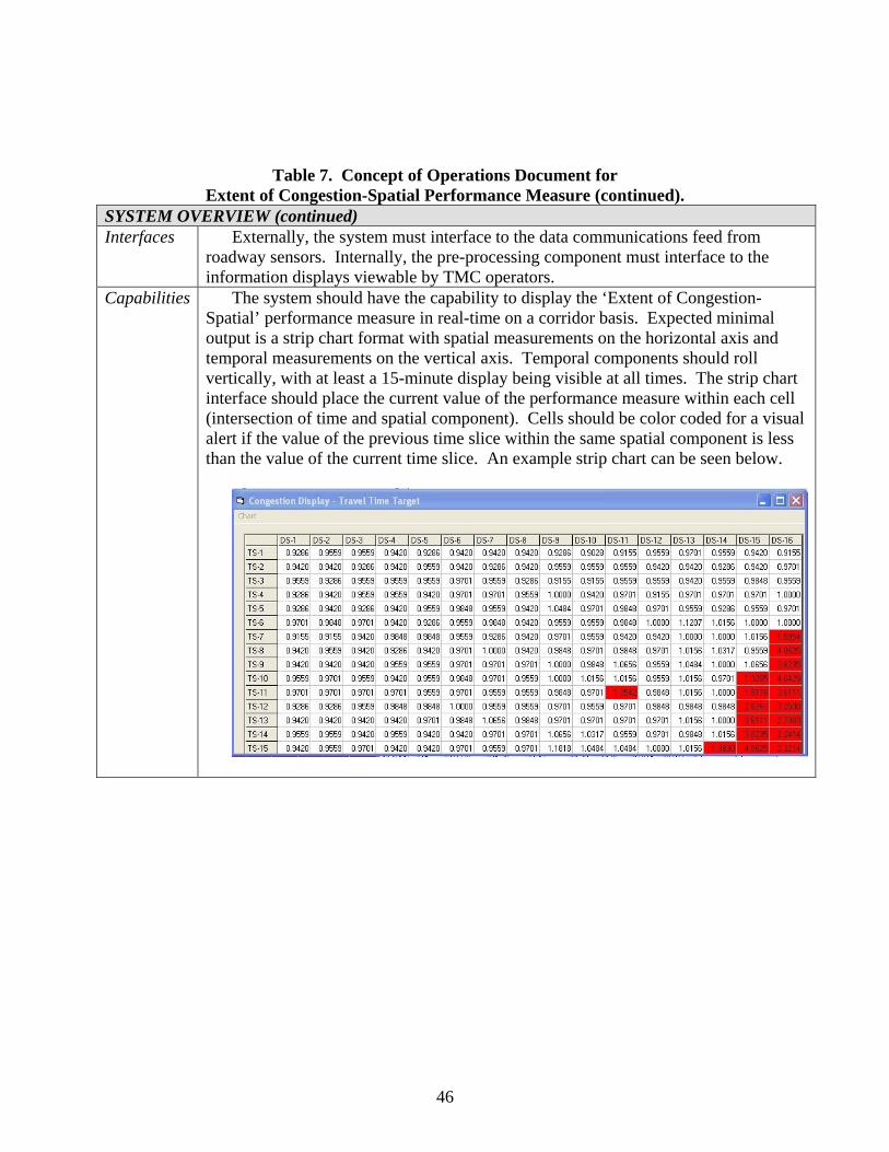
46

Table 7. Concept of Operations Document for Extent of Congestion-Spatial Performance Measure (continued).

SYSTEM OVERVIEW (continued)Interfaces Externally, the system must interface to the data communications feed from

roadway sensors. Internally, the pre-processing component must interface to the information displays viewable by TMC operators.

Capabilities The system should have the capability to display the ‘Extent of Congestion-Spatial’ performance measure in real-time on a corridor basis. Expected minimal output is a strip chart format with spatial measurements on the horizontal axis and temporal measurements on the vertical axis. Temporal components should roll vertically, with at least a 15-minute display being visible at all times. The strip chart interface should place the current value of the performance measure within each cell (intersection of time and spatial component). Cells should be color coded for a visual alert if the value of the previous time slice within the same spatial component is less than the value of the current time slice. An example strip chart can be seen below.

CHAPTER 6: USING A MULTI-CRITERION APPROACH TO SELECT

PERFORMANCE MEASURES

Selecting freeway performance measures is an especially complex and difficult process

that requires considering the different aspects influencing freeway operations. Furthermore,

construction funds, labor, and materials are becoming increasingly scarce, which reduces the

possibility of decreasing congestion problems by increasing capacity (4). Thus, traffic operations

management plays an important role in alleviating traffic congestion, improving safety, and

improving mobility in existing freeway systems. Operations management strategies used for

freeway systems include traffic incident detection, traveler information systems, managed lanes,

ramp management, etc. In order to evaluate freeway performance before and after any of these

operational strategies are applied, measures of effectiveness (MOEs), such as density, speed, and

volume (5) and the travel time index (6), are utilized. The quality of these performance

measures depends on the equipment and data collection techniques used.

Transportation planners must determine whether equipment and data collection

techniques should be provided in specific locations or exclusively when incidents occur; some

equipment can provide performance measure data without additional investment. For example,

existing loop detectors can provide spot speeds at specific locations, which enable a planner to

track improvements at a particular location. Recently, NCHRP Synthesis 311 (1) has developed

a scoring approach to assess the strengths and weakness of performance measures. The

qualitative criteria that are used for evaluating the performance measures include clarity and

simplicity, descriptive and predictive ability, analysis capacity, accuracy and precision, and

flexibility. These criteria may do a good job assessing performance measure quality in a general

sense; however, they do not provide a strong approach for identifying preferred performance

measures based on specific local characteristics, such as the reliability and accuracy of different

data collection strategies for the same performance measure. In addition, when choosing a

particular performance measure, there will likely be costs associated with either collecting the

data necessary for generating the performance measure in the first place or on-going operational

costs associated with tracking and maintaining the performance measure data itself. At a local

level for specific constraints and conditions, the decision-making criteria should include

47

48

commensurate quantitative criteria because decision-makers are unlikely to arrive at the

preferred alternative when using only general assessments of qualitative criteria.

This report provides a decision-making framework for assisting transportation planners

and operators in selecting alternative freeway performance measures based on both qualitative,

such as understanding, measurability, availability, and importance, and quantitative measures,

such as time, cost, accuracy, and reliability. This research considers the scoring of qualitative

criteria in NCHRP 311 (1) as a potential starting point for selecting among alternative

performance measures where the decision-makers can decide whether to consider or reject a

performance measure based on its score for qualitative criteria; the decision makers can establish

minimum performance thresholds for the qualitative criteria, and all alternative performance

measures that fail to meet or exceed these thresholds for all criteria will be excluded from further

consideration. The remaining candidate performance measures still must be evaluated for the

local characteristics using quantitative criteria. Decision-makers may establish similar

performance thresholds for the quantitative criteria and use them for screening as well. After all

screening is complete, the authors propose using a multi-criteria decision model (MCDM), such

as Simple Additive Weighting (SAW) and ELECTRE III, to combine quantitative criteria for

evaluating the performance measures. A MCDM ranks the alternatives for the decision-makers

to make their final selection. The approach that this report proposes improves on existing

techniques by adding a screening stage and integrating quantitative criteria that can handle local

characteristics. These improvements make the approach viable for local decision-makers who

must choose freeway operational performance measures under constrained conditions, such as

budget or personnel. In the following chapters, the proposed methodology is discussed in detail

and presented with an example of its application.

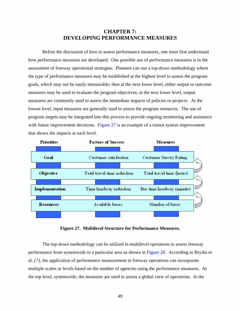
CHAPTER 7: DEVELOPING PERFORMANCE MEASURES

Before the discussion of how to assess performance measures, one must first understand

how performance measures are developed. One possible use of performance measures is in the

assessment of freeway operational strategies. Planners can use a top-down methodology where

the type of performance measures may be established at the highest level to assess the program

goals, which may not be easily measurable; then at the next lower level, either output or outcome

measures may be used to evaluate the program objectives; at the next lower level, output

measures are commonly used to assess the immediate impacts of policies or projects. At the

lowest level, input measures are generally used to assess the program resources. The use of

program targets may be integrated into this process to provide ongoing monitoring and assistance

with future improvement decisions. Figure 27 is an example of a transit system improvement

that shows the impacts at each level.

Figure 27. Multilevel Structure for Performance Measures.

The top-down methodology can be utilized in multilevel operations to assess freeway

performance from systemwide to a particular area as shown in Figure 28. According to Brydia et

al. (7), the application of performance measurement in freeway operations can incorporate

multiple scales or levels based on the number of agencies using the performance measures. At

the top level, systemwide, the measures are used to assess a global view of operations. In the

49

next lower level, called the interagency level, many agencies will share resources in order to

improve their operational programs, such as incident management and air quality. The third

level, daily operations, focuses on Transportation Management Center operations, such as lane

shifts, dynamic messages, signal timing, and ramp metering. TMC operators may use these

measures to assess their programs and strategies. At the bottom level, the measures are used to

assess equipment or discrete elements of the transportation system, such as equipment reliability.

Since the performance measures can be used in multiple scales, good performance measures

should be able to assess the freeway performance in multiple scales also. For example,

performance measures used to assess at the systemwide level should also apply at the

interagency level. In addition, performance measures for equipment should be used to evaluate

potential performance measures for daily operation.

Figure 28. Multilevel Operation Approach.

Since performance measurement has been used in many fields, there is no single

methodology or exact rule for selecting specific measures. In addition, criteria for selecting

appropriate performance measures should be decided by the people who are involved in the

performance measurement program, such as those who collect and use the data or experts who

understand the strengths and limitations of each performance measure. Good performance

measures in general should focus on the goals and objectives of the program whose performance

50

51

is to be assessed. They should be simple, easy to understand for everyone, able to respond to the

changes in the system, inexpensive to obtain, organizationally acceptable, credible, timely,

comparable, compatible, customer focused, consistent, measurable, available, balanced, valuable,

and practical (7, 8, 9). The following chapters provide a framework for weighing performance

measures to choose the optimal measure for the application.

CHAPTER 8: PERFORMANCE MEASURE CREATION AND SELECTION

METHODOLOGY

The five steps developed in this methodology focus on the roles of decision makers and

coordinators in creating and screening performance measures. The decision makers are defined

as the individuals responsible for using the performance measures for evaluating freeway

operational strategies, while the coordinators are defined as individuals who assist the decision

makers by guiding the process and conducting any necessary analysis during the performance

measure selection process. Figure 29 shows the methodology.

STEP 1: ESTABLISH THE “DECISION STATEMENT”

Specifying the proper “decision statement” is a crucial step for the decision makers

because it can determine if the solution meets the desired goal. In addition, the established

decision statement will lead the solutions to be “simple versus complex” or “broad versus

narrow.” For example, a decision statement: “select a strategy to reduce traffic congestion on a

freeway” will provide a solution of only the one best strategy. However, if the decision

statement is changed to “select strategies to reduce traffic congestion on a freeway,” this may

lead to the consideration of various strategies, which minimize traffic congestion on a freeway.

The roles of decision makers and coordinators involved in this step are:

• Decision makers have to clarify the objective by identifying a problem and

establishing a decision statement in order to scope the problem’s boundary and

feasible solutions. A problem can cause various challenges, for example, traffic

congestion may lead to environmental externalities, such as air pollution. Thus,

decision makers should focus on the main cause of the problem rather than the

outcomes of the problem.

• Coordinators should ensure that the results of the discussion will lead to the main

cause of the problem. They should provide useful information, which includes

traffic condition data, travel behavior, on-road activities, etc.

53

Figure 29. Decision-Making Process.

STEP 2: IDENTIFY THE “SET OF ALTERNATIVES OR SOLUTIONS”

Once a decision statement is identified, the decision makers must clearly understand the

program goals and performance measures. They must establish the possible alternatives or

solutions based on the decision statement described in Step 1. The roles of the decision makers

and coordinators involved in this step are:

• Decision makers must establish the feasible alternatives or solutions.

• Coordinators should provide any additional information as needed. The useful

information will enhance decision makers’ viewpoints in the selection of feasible

54

alternatives or solutions. To accomplish this, coordinators may conduct a survey

for the decision makers that may include the following questions:

• What are the objectives of the program?

• What are the current operational performance measures used in the program?

• What operational performance measures do you expect to be applied in the

future?

• The purpose of providing the program objectives is to make sure that the

decision makers consider these objectives when generating possible

alternatives.

STEP 3: ESTABLISH THE “SET OF CRITERIA USED FOR ASSESSING PERFORMANCE MEASURE BASED ON EQUIPMENT AND DATA COLLECTION TECHNIQUES ON FREEWAY SYSTEMS”

Once the set of feasible alternatives is generated in Step 2, the set of constraints for

assessing the feasible alternatives should be established. The set of constraints may include

qualitative and quantitative criteria. The qualitative criteria will be used to determine the

possibility of assessing the performance measures, and they may include measurability,

comprehension, and availability. The quantitative criteria may include budget constraints or

limitations of equipment and data collection techniques. The roles of the decision makers and

coordinators involved in this step are:

• Decision makers have to identify the “set of constraints” for assessing the quality of

the freeway performance measures in the next step. They should indicate the

critical criteria.

• Coordinators should provide any additional information, especially information that

enhances the decision makers’ criteria selection, as needed. The information

should include the limitations of the feasible alternatives provided in the previous

step. The possible decision maker questions include:

• What are the current performance measures used in the program at the system

wide, interagency, daily operation, or equipment level?

• What factors affect the use of those performance measures?

55

The coordinators may propose some potential criteria, which provide decision makers a

starting point. Then, the decision makers must choose to accept or reject these proposed criteria,

or provide alternate criteria. This process assists the decision makers’ criteria selection. An

example of a questionnaire is illustrated in Figure 30; however, the complete questionnaire is

provided in Appendix A. Note that in Figure 30 blank spaces are available, indicating the

availability of decision makers to include their own criteria.

Figure 30. The Hierarchy of Criteria for Performance Measures.

Within Steps 2 and 3, various techniques, such as brainstorming, nominal group

technique (NGT), surveys, or the Delphi method may be used to generate feasible alternatives

and their criteria. Coordinators need to select the proper technique for the particular situation

because each technique has its own advantages and limitations. For example, according to

Ababutain (10), the objective of brainstorming is to generate all possible ideas in order to

enhance the possibility of reaching ideal solutions. Thus, the final results may generate an

unlimited number of solutions; however, the limitation of brainstorming occurs when some

members of the group have strong opinions, which lead the other members to quickly reach an

agreement without a complete discussion. Thus, the results may not include other potentially

better solutions. Unlike the brainstorming technique, the NGT uses a questionnaire survey to

56

allow decision makers to communicate in writing, which can avoid preliminary arguments.

However, surveys that allow face-to-face and phone interviews may create conforming

influences and decrease the possibility of generating ideas freely. Because the selection of

freeway operational strategies decision uses experts who are directly involved with the freeway

management system, the researchers selected the Delphi method. According to Dalkey and

Helmer (11), coordinators will select the respondents from a group of experts that will be asked

intensive questions with controlled opinion feedback. Disagreements among the experts will

develop successive iterations until the various opinions yield to a widely acceptable view. The

process ends at this point. The success of this method depends on experts’ knowledge,

experiences, and viewpoints that can reflect the true value of whatever they judge. For example,

constructing a new freeway can provide both advantages and disadvantages depending on the

experts’ viewpoints. A new freeway can reduce traffic congestion; however, it can induce new

vehicles to use it and increase on-road emissions.

STEP 4: SCREENING THE “SET OF ALTERNATIVES OR SOLUTIONS IN STEP 2”

Quality is better than quantity. More performance measures do not mean that they will

provide a better assessment of the program. Thus, Step 4 provides an approach for screening the

alternatives that are identified in Step 2. The processes include grouping the performance

measures, defining the direct or proxy performance measures, setting the constraints, and

eliminating performance measures based on minimum assessment levels established by the

decision makers.

Step 4.1: Grouping the Alternatives that Convey the Same Meaning

In order to avoid using redundant performance measures, the performance measures that

convey the same meaning must be grouped. For example, when planners consider the human

health impacts due to traffic congestion, the Air Quality Index (AQI) used in the United States

and the Air Quality Health Index (AQHI) used in European countries are indicators for assessing

ambient air quality, which affects human health. However, both indices convey the same

meaning; to be practical, decision makers should select either AQI or AQHI, but not both. The

coordinators must clearly understand the definition of the alternatives obtained in Step 2 before

they group them.

57

Step 4.2: Defining Direct or Proxy Performance Measures

Ideally, decision makers should consider direct performance measures before resorting to

proxy performance measures. Good performance measures should be a direct consequence of

activities. For example, if the desired result is minimizing traffic congestion, traffic volume

should be a good performance measure (direct consequence). A proxy measure, such as vehicle

registration, may sometimes be used in the absence of suitable performance measures due to

time, budget constraints, or data unavailability. Unfortunately, a proxy measure may not provide

a good result because it relies on strong correlation between the factors. The coordinators have

to define the performance measures in Step 4.1 as either direct or proxy measures.

Step 4.3: Setting the Constraints for Screening the Alternatives

Qualitative criteria and quantitative criteria will be used to screen the feasible

performance measures in the next step. Both qualitative and quantitative criteria established in

Step 3 may have either a minimum or maximum acceptable value for each criterion, which

represents the threshold that the performance measures must reach. The decision makers have to

establish the set of constraints and their thresholds.

Step 4.4: Eliminating the Alternatives by Aspects

As developed in NCHRP Synthesis 311 (1), Table 8 details a scoring approach to assess

the strengths and weakness of various measures based on the qualitative criteria and sub-criteria.

58

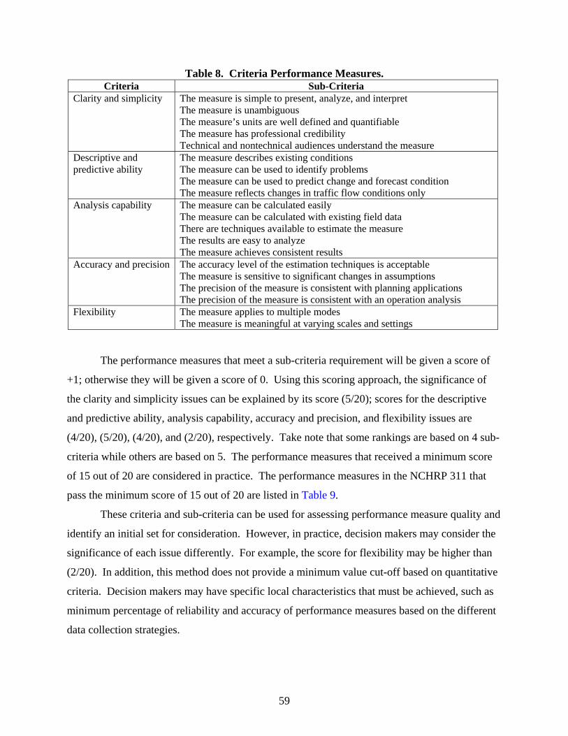
59

Table 8. Criteria Performance Measures. Criteria Sub-Criteria

Clarity and simplicity The measure is simple to present, analyze, and interpret The measure is unambiguous The measure’s units are well defined and quantifiable The measure has professional credibility Technical and nontechnical audiences understand the measure

Descriptive and predictive ability

The measure describes existing conditions The measure can be used to identify problems The measure can be used to predict change and forecast condition The measure reflects changes in traffic flow conditions only

Analysis capability The measure can be calculated easily The measure can be calculated with existing field data There are techniques available to estimate the measure The results are easy to analyze The measure achieves consistent results

Accuracy and precision The accuracy level of the estimation techniques is acceptable The measure is sensitive to significant changes in assumptions The precision of the measure is consistent with planning applications The precision of the measure is consistent with an operation analysis

Flexibility The measure applies to multiple modes The measure is meaningful at varying scales and settings

The performance measures that meet a sub-criteria requirement will be given a score of

+1; otherwise they will be given a score of 0. Using this scoring approach, the significance of

the clarity and simplicity issues can be explained by its score (5/20); scores for the descriptive

and predictive ability, analysis capability, accuracy and precision, and flexibility issues are

(4/20), (5/20), (4/20), and (2/20), respectively. Take note that some rankings are based on 4 sub-

criteria while others are based on 5. The performance measures that received a minimum score

of 15 out of 20 are considered in practice. The performance measures in the NCHRP 311 that

pass the minimum score of 15 out of 20 are listed in Table 9.

These criteria and sub-criteria can be used for assessing performance measure quality and

identify an initial set for consideration. However, in practice, decision makers may consider the

significance of each issue differently. For example, the score for flexibility may be higher than

(2/20). In addition, this method does not provide a minimum value cut-off based on quantitative

criteria. Decision makers may have specific local characteristics that must be achieved, such as

minimum percentage of reliability and accuracy of performance measures based on the different

data collection strategies.

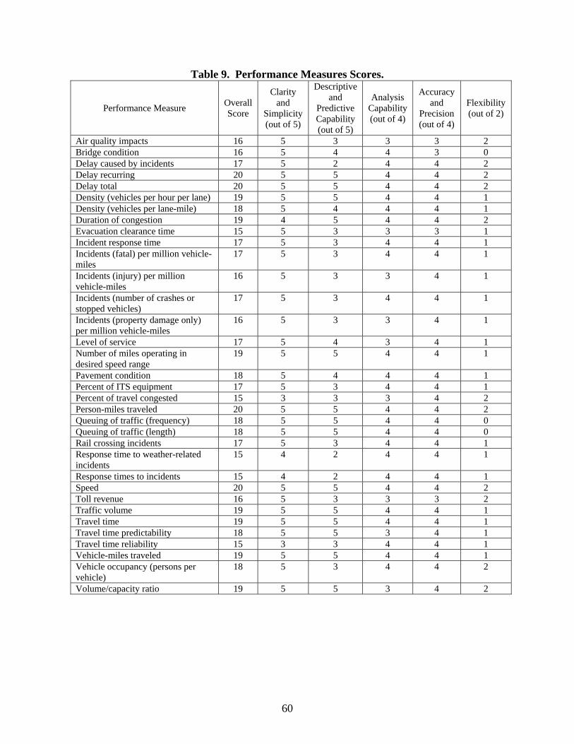
Table 9. Performance Measures Scores. Descriptive

and Predictive Capability (out of 5)

Accuracy and

Precision (out of 4)

Clarity and

Simplicity

Analysis Capability Flexibility

(out of 2) Overall Score Performance Measure

(out of 4) (out of 5)

Air quality impacts 16 5 3 3 3 2 Bridge condition 16 5 4 4 3 0 Delay caused by incidents 17 5 2 4 4 2 Delay recurring 20 5 5 4 4 2 Delay total 20 5 5 4 4 2 Density (vehicles per hour per lane) 19 5 5 4 4 1 Density (vehicles per lane-mile) 18 5 4 4 4 1 Duration of congestion 19 4 5 4 4 2 Evacuation clearance time 15 5 3 3 3 1 Incident response time 17 5 3 4 4 1 Incidents (fatal) per million vehicle-miles

17 5 3 4 4 1

Incidents (injury) per million vehicle-miles

16 5 3 3 4 1

Incidents (number of crashes or stopped vehicles)

17 5 3 4 4 1

Incidents (property damage only) per million vehicle-miles

16 5 3 3 4 1

Level of service 17 5 4 3 4 1 Number of miles operating in desired speed range

19 5 5 4 4 1

Pavement condition 18 5 4 4 4 1 Percent of ITS equipment 17 5 3 4 4 1 Percent of travel congested 15 3 3 3 4 2 Person-miles traveled 20 5 5 4 4 2 Queuing of traffic (frequency) 18 5 5 4 4 0 Queuing of traffic (length) 18 5 5 4 4 0 Rail crossing incidents 17 5 3 4 4 1 Response time to weather-related incidents

15 4 2 4 4 1

Response times to incidents 15 4 2 4 4 1 Speed 20 5 5 4 4 2 Toll revenue 16 5 3 3 3 2 Traffic volume 19 5 5 4 4 1 Travel time 19 5 5 4 4 1 Travel time predictability 18 5 5 3 4 1 Travel time reliability 15 3 3 4 4 1 Vehicle-miles traveled 19 5 5 4 4 1 Vehicle occupancy (persons per vehicle)

18 5 3 4 4 2

Volume/capacity ratio 19 5 5 3 4 2

60

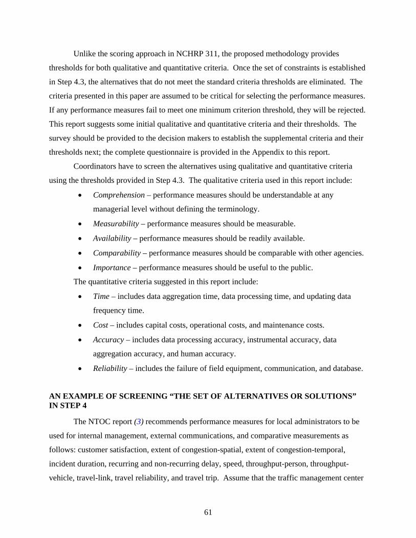
Unlike the scoring approach in NCHRP 311, the proposed methodology provides

thresholds for both qualitative and quantitative criteria. Once the set of constraints is established

in Step 4.3, the alternatives that do not meet the standard criteria thresholds are eliminated. The

criteria presented in this paper are assumed to be critical for selecting the performance measures.

If any performance measures fail to meet one minimum criterion threshold, they will be rejected.

This report suggests some initial qualitative and quantitative criteria and their thresholds. The

survey should be provided to the decision makers to establish the supplemental criteria and their

thresholds next; the complete questionnaire is provided in the Appendix to this report.

Coordinators have to screen the alternatives using qualitative and quantitative criteria

using the thresholds provided in Step 4.3. The qualitative criteria used in this report include:

• Comprehension – performance measures should be understandable at any

managerial level without defining the terminology.

• Measurability – performance measures should be measurable.

• Availability – performance measures should be readily available.

• Comparability – performance measures should be comparable with other agencies.

• Importance – performance measures should be useful to the public.

The quantitative criteria suggested in this report include:

• Time – includes data aggregation time, data processing time, and updating data

frequency time.

• Cost – includes capital costs, operational costs, and maintenance costs.

• Accuracy – includes data processing accuracy, instrumental accuracy, data

aggregation accuracy, and human accuracy.

• Reliability – includes the failure of field equipment, communication, and database.

AN EXAMPLE OF SCREENING “THE SET OF ALTERNATIVES OR SOLUTIONS” IN STEP 4

The NTOC report (3) recommends performance measures for local administrators to be

used for internal management, external communications, and comparative measurements as

follows: customer satisfaction, extent of congestion-spatial, extent of congestion-temporal,

incident duration, recurring and non-recurring delay, speed, throughput-person, throughput-

vehicle, travel-link, travel reliability, and travel trip. Assume that the traffic management center

61

(TMC) or third level in Figure 28 will use speed as one of the alternative performance measures

for a freeway system. The screening approach outlined in Step 4 should be applied as follows.

Step 4.1: Grouping The Alternatives That Convey The Same Meaning

Speed can be divided into two groups: spot speed and space mean speed. Spot speed is

described as an instantaneous speed measured at a specific location, while space mean speed is

an average travel speed over a distance. The equipment and techniques used for collecting spot

and space mean speed data are:

• Spot speed - gun radar, loop detector, microwave sensor, video sensor, infrared

sensor, and acoustic sensor.

• Space mean speed - test vehicle (floating car) technique, license plate matching

technique, video matching technique, ITS probe vehicle technique, time lapse

photography, and toll tag matching technique.

Step 4.2: Defining Direct or Proxy Performance Measures

Both spot speed and space mean speed are defined as direct performance measures.

Step 4.3: Setting the Constraints for Screening the Alternatives

When considering qualitative criteria, speed should be an appropriate performance

measure, which can be understood by most people; moreover, it is measurable because speed

data can be collected using a variety of data collection techniques. Lastly, it can be compared

between agencies and is useful for the general public. When considering quantitative criteria, the

study proposes that decision makers use the accuracy, reliability, and data processing time as

constraining criteria. The data collection for accuracy and reliability should be higher than 95

percent and 85 percent, respectively; data processing should be less than 15 minutes.

Step 4.4: Eliminating the Alternatives by Aspects

In the absence of valid data, the accuracy constraint is omitted, so decision makers will

consider the data collection strategies that have reliability above 95 percent and data processing

less than 15 minutes. Figure 31 illustrates the results when screening criteria by minimum

performance thresholds. The alternatives that do not meet some specified standard are eliminated

until the remaining alternatives, which pass all constraints, fall in the shaded area.

62

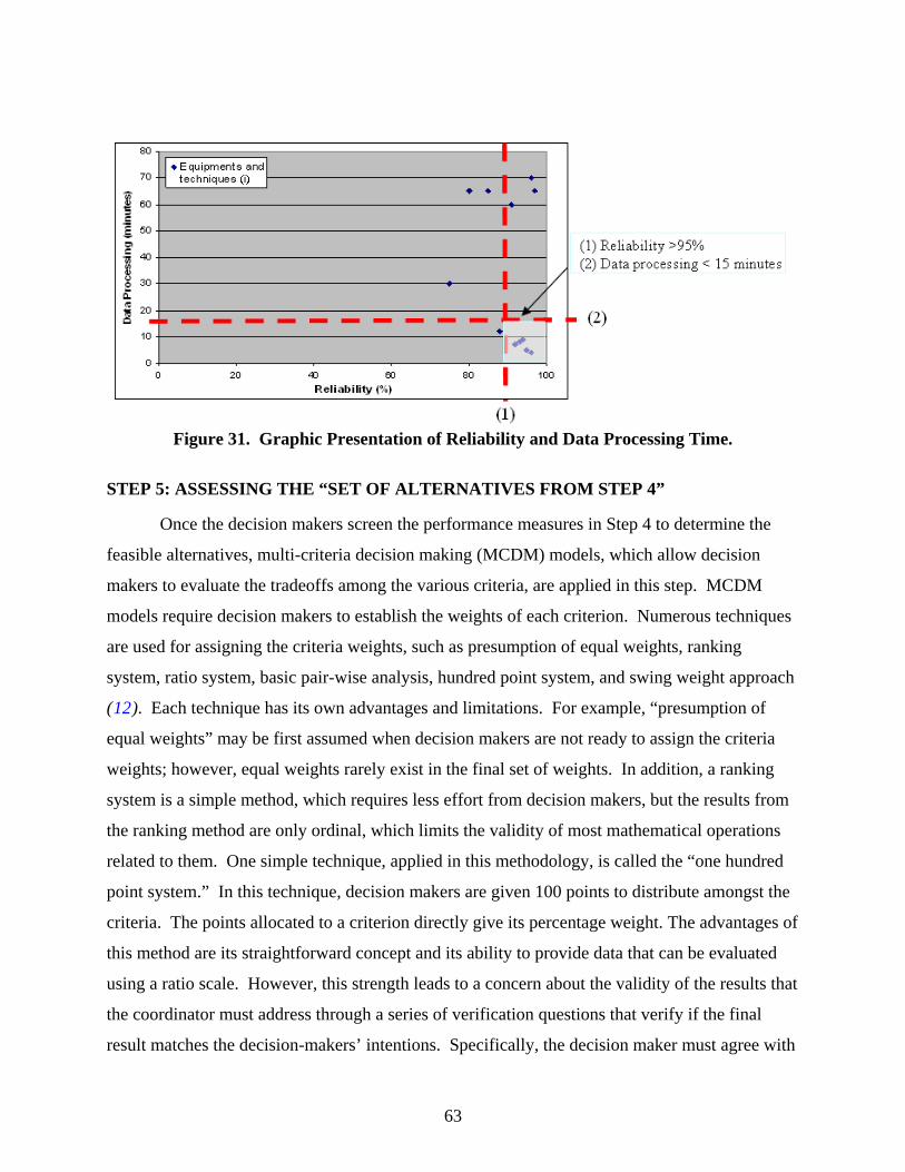
Figure 31. Graphic Presentation of Reliability and Data Processing Time.

STEP 5: ASSESSING THE “SET OF ALTERNATIVES FROM STEP 4”

Once the decision makers screen the performance measures in Step 4 to determine the

feasible alternatives, multi-criteria decision making (MCDM) models, which allow decision

makers to evaluate the tradeoffs among the various criteria, are applied in this step. MCDM

models require decision makers to establish the weights of each criterion. Numerous techniques

are used for assigning the criteria weights, such as presumption of equal weights, ranking

system, ratio system, basic pair-wise analysis, hundred point system, and swing weight approach

(12). Each technique has its own advantages and limitations. For example, “presumption of

equal weights” may be first assumed when decision makers are not ready to assign the criteria

weights; however, equal weights rarely exist in the final set of weights. In addition, a ranking

system is a simple method, which requires less effort from decision makers, but the results from

the ranking method are only ordinal, which limits the validity of most mathematical operations

related to them. One simple technique, applied in this methodology, is called the “one hundred

point system.” In this technique, decision makers are given 100 points to distribute amongst the

criteria. The points allocated to a criterion directly give its percentage weight. The advantages of

this method are its straightforward concept and its ability to provide data that can be evaluated

using a ratio scale. However, this strength leads to a concern about the validity of the results that

the coordinator must address through a series of verification questions that verify if the final

result matches the decision-makers’ intentions. Specifically, the decision maker must agree with

63

64

the ratio scale implications of their weights. The roles of the decision makers and coordinators

involved in this step are:

• Decision makers have to establish the criteria weights through one of the weighting

techniques described above. MCDM models will be used to assess those

alternatives in the final decision-making process.

• Coordinators have to provide additional questions to assess the consistency of the

results of the weighting technique used. For example, within the “one hundred

point system” approach, decision makers must understand the comparisons and

ratios between the criteria.

CHAPTER 9: MULTI-CRITERIA DECISION-MAKING MODELS

Selecting performance measures is usually based on more than one criterion. Using a

MCDM approach allows decision makers to analyze complex decision problems with usually

conflictive and opposite points of view. Additionally, this type of analysis can be used to

evaluate performance measures when their attributes are not valued in monetary terms (12).

According to Polatidis et al. (13), there are two main families of MCDM models: utility

function-based models and outranking methods. The utility function-based models include

Multi-Attribute Utility Theory (MAUT) (14), Analytic Hierarchy Process (AHP) (15), and

Simple Additive Weighting (SAW). Outranking methods include the ELECTRE families (16,

17), PROMETHEE I and II methods (18), and Regime Method Analysis (19). Some models,

such as Stochastic Multiobjective Acceptability Analysis (SMAA) (20), Novel Approach to

Imprecise Assessment and Decision Environment (NAIDA) (21), and Flag Model (22), do not

fit into either of these broad families.

All MCDM models can provide the ranking of alternatives, but none of them can be

described to fit decision problems completely. For example, SAW uses a simple utility function

model, which requires high quality of data (using real data or actual scores); however, decision

makers may only require a ranking of the alternatives rather than their actual scores. Unlike the

SAW model, AHP’s use of pairwise comparisons allows decision makers to establish the ranking

of alternatives when actual information is unavailable; unfortunately, within the AHP approach,

decision makers may have a difficult time making all of the necessary comparisons. The

concordance methods do not require decision makers to weight the importance of one criterion

against the others. This method may provide only a partial ranking and preferred options rather

than one best option. The selected MCDM methods should fit the complexity of problems,

availability of data, and weighting technique. The authors provide an application of the SAW

and ELECTRE III methods, which are assumed to fit with the available data and decision

problems.

65

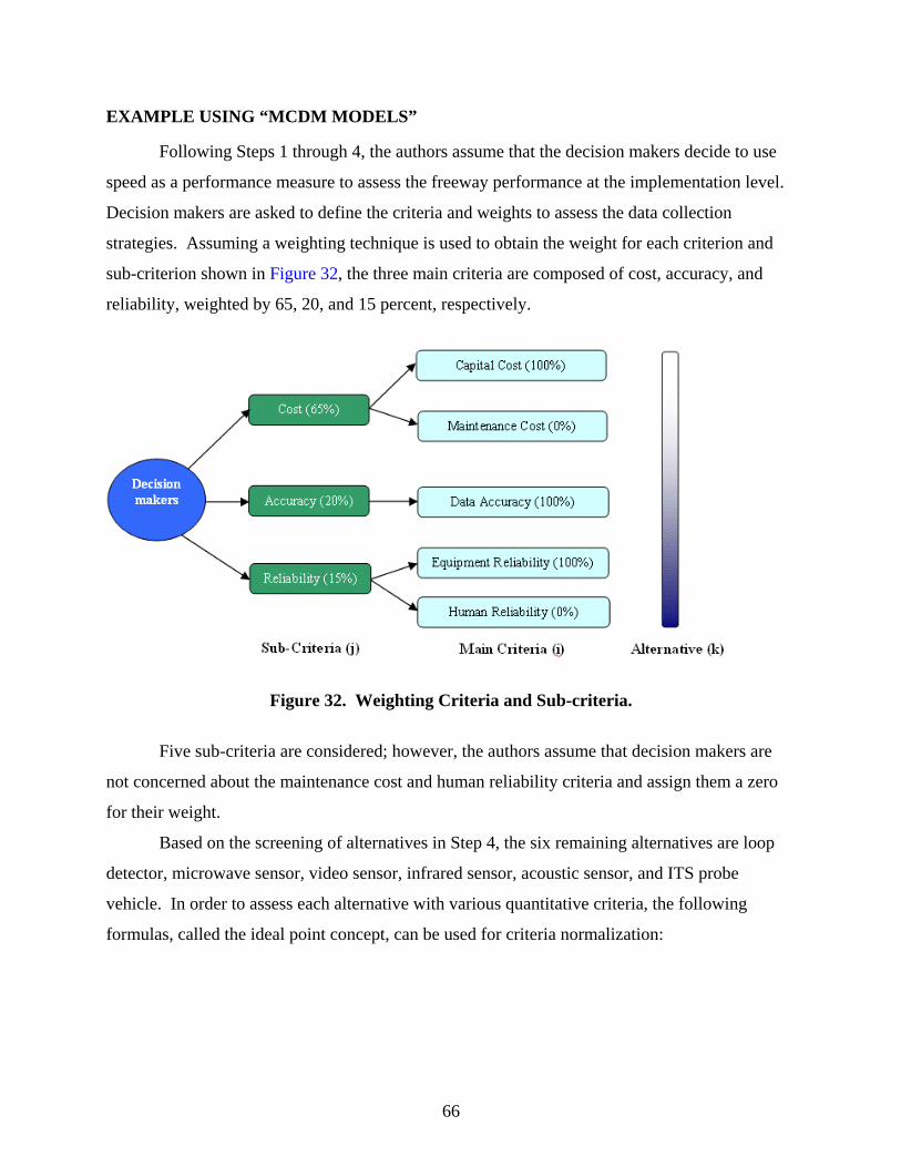
EXAMPLE USING “MCDM MODELS”

Following Steps 1 through 4, the authors assume that the decision makers decide to use

speed as a performance measure to assess the freeway performance at the implementation level.

Decision makers are asked to define the criteria and weights to assess the data collection

strategies. Assuming a weighting technique is used to obtain the weight for each criterion and

sub-criterion shown in Figure 32, the three main criteria are composed of cost, accuracy, and

reliability, weighted by 65, 20, and 15 percent, respectively.

Figure 32. Weighting Criteria and Sub-criteria.

Five sub-criteria are considered; however, the authors assume that decision makers are

not concerned about the maintenance cost and human reliability criteria and assign them a zero

for their weight.

Based on the screening of alternatives in Step 4, the six remaining alternatives are loop

detector, microwave sensor, video sensor, infrared sensor, acoustic sensor, and ITS probe

vehicle. In order to assess each alternative with various quantitative criteria, the following

formulas, called the ideal point concept, can be used for criteria normalization:

66

ijkijk

ijkijkijk xx

xxC

minmaxmin−

−= Eq. 13

ijkijk

ijkijkijk xx

xxC

minmaxmax

−

−= Eq. 14

Where:

xijk is the score of alternative k with respect to criteria i on sub-criteria j,

Cijk indicates the benefit of performance measure.

After normalization, all criteria are positive criteria where a higher Cijk is preferred.

Within the ideal point concept, the quantitative data are converted into a comparable unit

between “0 and 1” where “0” is the lowest utility value. The use of Eq. 13 and Eq. 14 depend on

the variable xijk. If an increase of xijk leads to improvement, then Eq. 13 is used; otherwise,

Eq. 14 is applied. For example, if xijk is travel time, an alternative that leads to the increase of

travel time will be unfavorable and Eq. 13 is used. Eq. 13 and Eq. 14 are applied in this example

and the scaling values are shown in Table 10, which is used for the SAW and ELECTRE III

methods.

SAW METHOD

In Figure 32, the decision hierarchies are composed of two levels: main criteria (level i)

and sub-criteria (level j). The form of an additive utility function in the upper level (i) is:

∑=

=n

ijkiktot UwV

1 Eq. 15

Where:

Vtot is the overall valuation for alternative k; wik is the weight assigned to criterion i for

alternative k; Ujk is the utility in the lower level j for alternative k; and n is the number of

criteria. The utility function in the lower level is calculated as follows:

67

∑=

=m

jijkjkjk CwU

1' Eq. 16

Where:

Ujk is the utility in the lower level j for alternative k; m is the number of sub-criteria of

criterion j; w’jk is the weight assigned to sub-criterion j; Cijk is the scaling value calculated

from Eq. 13 or Eq. 14. The final decision is based on the result from the overall valuation

in Eq. 15.

Table 10. Scaling Value for the Alternatives. Loop Detector

Microwave Sensor

Video Sensor

Infrared Sensor

Acoustic Sensor

ITS Probe Vehicle Sub-Criteria

Capital Cost ($) 14,400 13,000 13,000 20,000 5,600 100,000 Data Accuracy (%) 95 95 95 90 90 90 Equipment Reliability (%) 95 95 95 95 92.5 96

Scaling the sub-criteria using Eq. 13 and Eq. 14. Data Accuracy 0.91 0.92 0.92 0.85 1.00 0.00 Equipments Reliability 1.00 1.00 1.00 0.00 0.00 0.00

Capital Cost 0.71 0.71 0.71 0.71 0.00 1.00

ELECTRE III METHOD

The ELECTRE III method uses the concept of a concordance and discordance index to

obtain alternative rankings. A concordance index Cj(a,b) for any pair of alternatives implies that

alternative a is at least as good as alternative b. Then, the concordance index is calculated as

follows:

Cj (a,b) = ∑=

n

jj bacw

1),( Eq. 17

Where:

wj is the relative importance of the different criteria.

c(a,b) is the local concordance index.

68

1, if )()( bgqag jjj ≥+

0, if Eq. 18)()( bqpag jjj ≤+ ; otherwise

Cj (a,b) = 0, if )()( bqpag jjj ≤+ ; otherwise Eq. 19

jj

jjj

qppbgag

−

+− )()( Eq. 20

The discordance index is used to model the magnitude of the lack of compensation

between the criteria by using a veto threshold vj (constant threshold). A discordance index

dj(a,b) for each pair of alternatives implies no alternative a is better than alternative b. Then, the

discordance index is calculated as follows:

Eq. 21

The discordance indices of different criteria are not aggregated using the criteria weights

because each criterion is evaluated for discordance individually. The degree of outranking or

credibility index is defined as follows:

Eq. 22

Where: is a set of criteria for which > ),( baJ ),( baC),( baD j

The credibility index is used to assess the tradeoff between alternatives a and b.

Alternative a will outrank alternative b when is greater than a minimum ‘threshold’

value,

),( baS

λ , which is usually set at approximately 0.85. Then, a positive score +1 will be given to

alternative a. In contrast, a negative score -1 will be given to alternative b being outranked. The

final ranking will be established based on the total score through the process of descending and

ascending distillation. More explanation of ELECTRE III can be found in Rogers et al. (12).

69

Roy et al. (16) describes the value of the preference threshold (p) and indifference

threshold (q), which is set as the margins of uncertainty, error, or imprecision. The p and q

thresholds can be defined by the decision makers’ opinions. The p threshold is related to the

positive attitude that a decision-maker may have for a particular criterion’s score. In addition,

the q threshold is the point where decision makers perceive a difference between alternatives

(23). The veto threshold (v) can be set against the hypothesis that alternative a will usually be

better than b. Due to the fact that sometimes alternative a may be worse, or alternative b

outperforms alternative a, the veto threshold (v) always is set greater than the p threshold.

However, the estimation of the veto threshold is difficult and many studies, in practice, often

avoid using it. As a result, the credibility index for each pair of alternatives is assumed to be

equal to the concordance index (16).

This example avoids the use of the veto threshold. The decision makers perceive the

value of the p and q threshold as follows:

• Capital Cost – This is an important criterion with the maximum weight because it

relates directly to the availability of types of equipment, techniques, etc. Thus, the q

threshold is set to a “small” value (q = 0.15), while the preference threshold is set

twice as large (p = 0.30).

• Data Accuracy and Equipment Reliability – This relates to the quality of information

obtained. However, current technologies lead to only slight differences in

equipment accuracy and reliability. Thus, the q threshold is set to a “large” value (q

= 0.25), while the preference threshold is set twice as large, p = 0.50.

ANALYSIS OF RESULT

The full ranking of alternatives using the SAW model based on the scaling data (Table

10) and weighting criteria (Figure 32) are analyzed. From this analysis, the microwave and

video sensors appear to be the best alternative with the same highest score (0.91) for the SAW

method. Loop detector, infrared sensor, acoustic sensor, and ITS probe vehicle trail behind in

that order. The ELECTRE III model is utilized to assess the same alternatives and the

microwave and video sensors are again the best alternatives at the highest level; however, the

loop detector is also one of the top alternatives (Figure 33).

70

71

The rank order for the two techniques is very similar; however, ELECTRE III does not

provide a score for the alternatives as SAW does. This difference between the two techniques is

critical for the decision-makers and coordinators to consider. Recall specifically, the earlier

discussion regarding the decision statement in Step 1; the choices made at this stage will likely

determine the appropriate technique to apply in Step 5. The core concept behind the difference

in the two techniques is ELECTRE III’s assumption that small differences between alternatives

are indistinguishable from one another due to inherent uncertainties in the decision-making

process. As seen in Figure 33, the alternatives that share the same rank in ELECTRE III all have

very similar scores in the SAW technique.

Figure 33. Ranking of Alternatives by using SAW and ELECTRE III Method.

CHAPTER 10: CONCLUSIONS AND DISCUSSION

OPERATIONS

The research performed within the scope of this project provided the groundwork

feasibility test of using performance measures in real-time. Year One efforts indicated that real-

time performance measurement is not being done. An examination of two thrust areas,

operations and emissions, concluded that the operations area was a viable avenue to continue

development of a real-time performance monitoring capability. The emissions area was not

found to be viable for development of a real-time, narrowly focused monitoring architecture.

In Year Two, a prototype real-time performance monitoring system was developed. The

development of this prototype system encompassed the creation of a system architecture,

assessment of potential measures, simulation based testing of real-time measures, assessment of

results and future viability, prototype interfaces and data storage capabilities, and a concept of

operations to guide future development or implementation.

The prototype interfaces (operator displays) emphasize several points. First, the use of

the NTOC performance measures in real-time can, in fact, provide an understanding of roadway

conditions and serve as a baseline to visually communicate that information, on both a temporal

and spatial basis. Second, while the initial results are promising, a modification to the NTOC

methodology would be necessary for some measures, such as a straight comparison of speed or

travel time. Without a comparison baseline, the normal volatility in these parameters would

render them somewhat useless for identifying abnormal conditions. Finally, additional efforts

are necessary to determine the sensitivity of the measures to variations in traffic levels, changes

in the ratio value used, etc. Additionally, a determination of the sensitivity of the travel time

ratio performance measure should be made if the target travel time values change by time of day,

as determined by an operator.

MULTI-CRITERION SELECTION

The selection framework detailed in this report improves on earlier research by

facilitating the constrained selection of freeway operational performance measures. The process

allows decision makers to generate candidate solutions and criteria before using both qualitative

73

74

and quantitative performance thresholds, and reduce the possibilities to a set of feasible

alternatives. The use of MCDMs provides an opportunity for the decision makers to evaluate the

tradeoffs across the different criteria. The decision makers must select the appropriate weighting

techniques or MCDMs based on the complexity of their problem or the required results because

each technique and MCDM has both strengths and limitations. The proposed criteria and

application framework provides the guidelines for future applications by TxDOT. The

successful implementation of the proposed methodology requires complete and engaged

participation from the decision makers.

Implementation of this research will use actual decision maker input to generate realistic

criteria and their weights. Additionally, decision maker input is required to establish the proper

performance thresholds. Testing the process with decision maker participation will facilitate

revision of the framework to fully meet TxDOT needs. After using this framework for selecting

operational freeway performance measures, it can be modified so that it is able to evaluate

different operational strategies and recommend alternatives for selection. This future

improvement is critical for the selection of operational alternatives in real-time based on their

associated performance measures.

CHAPTER 11: REFERENCES

1 “Performance Measures of Operational Effectiveness for Highway Segments and Systems.” NCHRP Synthesis 311. Transportation Research Board, National Research Council, Washington, DC. http://www.trb.org/publications/nchrp/nchrp_syn_311.pdf. 2003. 2 How to Measure Performance. A Handbook of Techniques and Tools. U.S. Department of Energy, Special Projects Group. Oak Ridge, TN. http://www.orau.gov/pbm/documents/handbook1a.html. October 1995. 3 National Transportation Operations Coalition (NTOC) Performance Measurement Initiative. Final Report. July 2005. http://www.ntoctalks.com/ntoc/ntoc_final_report.pdf. Accessed multiple dates, April through September 2007. 4 Freeway Management and Operations Handbook: Final Report, U.S. Department of Transportation, Federal Highway Administration, September 2003 5 Highway Capacity Manual, Transportation Research Board, National Research Council, Washington, DC, 2000. 6 Tim, L., and Schrank, D., Urban Mobility Study, Texas Transportation Institute, May 2005, http://mobility.tamu.edu/ums/, Accessed June 26, 2007 7 Brydia, R. E., Schneider, W. H., Mattingly, S. P., Sattler, M. L., Upayokin, A., Operations-Oriented Performance Measures for Freeway Management Systems: Year 1 Report, Technical Report 0-5292-1, 2007, http://tti.tamu.edu/documents/0-5292-1.pdf, Accessed July 29, 2007. 8 Jiji, D., guide for good performance measure (Beyond S.M.A.R.T.*), October 2005, http://www.i95coalition.org/PDF/Library/PerformanceMeasures/Good%20Measures%20Guide-10-25-05%20from%20Dan%20Jiji.pdf, Accessed June 26, 2007. 9 Office of Management and Budget, Performance Measurement Challenge and Strategies, June 2003, http://www.whitehouse.gov/omb/part/challenges_strategies.html, Accessed June 26, 2007. 10 Ababutain, A. Y., A Multi-Criteria Decision-Making Model for Selection of BOT Toll Road Proposals Within The Public Sector, PhD Thesis, University of Pittsburgh, 2002. 11 Dalkey, N. C., and Helmer, O., An experimental application of the Delphi method to the use of experts. Management Science, Vol. 9, 1963, pp. 458-467 12 Rogers, M. G., Engineering Project Appraisal: The Evaluation of Alternative Development Schemes, Blackwell Science Ltd, 2001.

75

http://www.trb.org/publications/nchrp/nchrp_syn_311.pdf

http://www.orau.gov/pbm/documents/handbook1a.html

http://www.ntoctalks.com/ntoc/ntoc_final_report.pdf

http://mobility.tamu.edu/ums/

http://tti.tamu.edu/documents/0-5292-1.pdf

http://www.whitehouse.gov/omb/part/challenges_strategies.html

76

13 Polatidis, H., Haralambopoulos, D. A., Munda, G., and Vreeker, R., Selecting an Appropriate Multi-Criteria Decision Analysis Technique for Renewable Energy Planning, Energy Sources, Part B: Economics, Planning and Policy, Volume 1, pp. 181-193, 2006. 14 Keeney, R., and Raiffa, H., Decision with Multiple Objectives: Preferences and Value Trade-offs, New York: John Wiley & Sons, 1976. 15 Saaty, T. L., The Analytic Hierarchy Process: Planning, Priority Setting, Resource Allocation, New York: McGraw-Hill, 1980. 16 Roy, B., and Vincke, P., Multicriteria Analysis: Survey and New Directions, European Journal of Operational Research, Volume 8, 1981, pp. 207-218. 17 Vincke, P., Multicriteria Decision Aid, New York: Wiley, 1992. 18 Brans, J. P., and Vincke, P., A Preference Ranging Organization Method, The PROMETHEE Method for MCDM, Management Science, Volume 31, 1985, pp. 647-656. 19 Nijkamp, P., Rietvelt, P., and Voogd, H., Multi-Criteria Evaluation in Physical Planning, Amsterdam: North-Holland, 1990. 20 Lahdelma, R., Hokkanen, J., and Salminen, P., SMAA-Stochastic Multiobjective Accepability Analysis, European Journal of Operational Research Volume 106, 1998, pp. 137-143. 21 Munda, G., Multicriteria Evaluation in a Fuzzy Environment – Theory and Applications in Ecological Economics, Heidelberg: Physica-Verlag, 1995. 22 Nijkamp, P., and Vreeker, R., Sustainability Assessment of Development Scenarios: Methodology and Application to Thailand, Ecological Economics, Volume 33, 2000, pp. 7-27. 23 Goletsis, Y., Psarras, J., and Samouilisdis, J., Project Ranking in the Armenian Energy Sector Using a Multicriteria Method for Groups, Annals of Operations Research, Volume 120, 2003, pp. 135-157.

APPENDIX MULTI-CRITERIA SELECTION MODEL QUESTIONNAIRE

77

79

SURVEY DOCUMENT

This appendix contains a survey document distributed to the project monitoring

committee during the course of the research to help define both the qualitative and quantitative

aspects of the multi-criterion selection model formulation.

Ove

rvie

w o

f ass

essi

ng p

erfo

rman

ce m

easu

res b

y qu

antit

ativ

e an

d qu

alita

tive

crite

ria

Qua

ntita

tive

and

qual

itativ

e cr

iteria

are

use

d to

ass

ess

the

qual

ity o

f pe

rfor

man

ce m

easu

res.

Figu

re A

-1 i

llust

rate

s th

e hi

erar

chic

crit

erio

n fo

r

sele

ctin

g pe

rfor

man

ce m

easu

res.

Tim

e, c

ost,

accu

racy

and

relia

bilit

y co

nstra

ints

are

use

d as

qua

ntita

tive

crite

ria w

hich

are

qua

ntifi

able

, whe

reas

qual

itativ

e cr

iteria

inc

lude

und

erst

andi

ng,

mea

sura

bilit

y; a

vaila

bilit

y, c

ompa

rabi

lity,

and

im

porta

nce

(see

Fig

ure

A-1

). Th

e de

finiti

on o

f ea

ch

crite

rion

is d

escr

ibed

in T

able

A-1

.

80

Figu

re A

-1.

Hie

rarc

hic

crite

rion

for

sele

ctin

g pe

rfor

man

ce m

easu

res.

Table A-1. Description of quantitative and qualitative criteria. Main-criteria Sub-criteria Description

Time

Data aggregation time

is the time duration required to gather the appropriate amount of data

The processing data time

is the time required to calculate the performance measures after the operational center received all information.

Updating frequency time

is the time between real-time updates of the performance measures (Data aggregation time plus time for transferring the data from fields to operation center).

Cost

Capital costs

are one time total costs being expensed to collect the data necessary to calculate the performance measure. Capital costs include costs of land, buildings, construction, and equipment.

Operational costs

are costs related to operation of organization and equipment.

Maintenance costs

are costs of labor and parts to perform repairs. Maintenance costs may also be required to maintain the equipment and data.

Accuracy

Data processing accuracy

is the quality of value being estimated or calculated by computable systems compared with the actual value estimated by reliable computable systems.

Instrumental accuracy

is the quality of value being measured by field equipment compared with the actual value measured by reliable instrument.

Data aggregation

accuracy

is the quality of value being gathered by computers or humans compared with the actual value gathered by reliable approach.

Human accuracyis the quality of value being processed by humans compared with the actual value processed by reliable approach.

Reliability

Failure of field equipment

is the percentage of time the field equipment does not function properly in routine circumstances or in unexpected conditions.

Failure of communication

is the percentage of time the communication system does not function properly in routine circumstances or in unexpected conditions.

Failure of database

is the percentage of time the database system does not function properly in routine circumstances or in unexpected conditions.

Understanding

Level 1

understandable by only experts (no need to define the terminology)

Level 2

understandable by agencies or organization (people in agencies or organization that work in the program understand the measures without defining the terminology)

Level 3

understandable by public (most people understand it without defining the terminology) Note: Good performance measure should be understandable at any level without defining the terminology.

81

Table A-1. (Cont.) Description of quantitative and qualitative criteria.

Main-criteria Sub-criteria Description

Measurability Level 1 Immeasurable

Level 2 Measurable Note: Good performance measure should be measurable.

Availability

Level 1 Data unavailable

Level 2 Data available Note: Good performance measure should be readily available as a direct performance measure.

Comparability

Level 1 Incomparable with other agencies or standards

Level 2 Comparable with other agencies or standards Note: Good performance measure should be comparable with other agencies.

Importance

Level 1 Useful for a small group Level 2 Useful for agencies or organizations

Level 3 Useful for public Note: Good performance measure should be useful for public.

Example of question on screening criteria 1. Do you think that screening criteria being provided are acceptable and suitable for assessing

freeway operation?

Yes ___

NO ___

Please, suggest the minimum and maximum value for screening criteria in Table A-2 below:

Table A-2. The perception of decision makers’ criteria threshold. Criteria Criteria Threshold

Time

(seconds)

Maximum data aggregation time

Maximum processing data time

Maximum updating frequency time

Cost ($)

Maximum capital cost

Maximum operation cost

Maximum maintenance cost

Accuracy (%)

Minimum % accuracy of data processing

Minimum % accuracy of instrument

Minimum % accuracy of data aggregation process

Minimum % accuracy of human interface

Reliability

(%)

Minimum % reliability of equipment

Minimum % reliability of communication system

Minimum % reliability of database system

82

If the answer is “No”, please suggest and explain other screening criteria including the minimum

or maximum threshold which should be added.

(1)………………………………………………………………………………………….………

………………………………………………………………………………………………………

………………………………………………………………………………………………………

(2)………………………………………………………………………………………….………

………………………………………………………………………………………………………

………………………………………………………………………………………………………

(3)………………………………………………………………………………………….………

………………………………………………………………………………………………………

………………………………………………………………………………………………………

(4)………………………………………………………………………………………….………

………………………………………………………………………………………………………

………………………………………………………………………………………………………

(5)………………………………………………………………………………………….………

………………………………………………………………………………………………………

………………………………………………………………………………………………………

(6)………………………………………………………………………………………….………

………………………………………………………………………………………………………

………………………………………………………………………………………………………

(7)………………………………………………………………………………………….………

………………………………………………………………………………………………………

………………………………………………………………………………………………………

(8)………………………………………………………………………………………….………

………………………………………………………………………………………………………

………………………………………………………………………………………………………

83

Example of question on assessing performance measures by quantitative and qualitative criteria 2. Do you think that criteria for selecting performance measures should include qualitative

criteria?

Yes ___

NO ___

If the answer is “No”, please skip to question (4).

3. Do you think that qualitative criteria listed in Table A-1 are acceptable and suitable to assess

the performance measure for freeway operation?

Yes ___

NO ___

If the answer is “No”, please suggest other criteria which should be added (fill out in blank

box) or omitted (circle).

Main criteria

Qualitative criteria

Understanding Acceptable / unacceptable

Measurability Acceptable / unacceptable

Availability Acceptable / unacceptable

ComparabilityAcceptable / unacceptable

Importance Acceptable / unacceptable

…………..

…………..

More criteria ………………………………………………………………………………..

Comments …………………………………………………………………………………………..

………………………………………………………………………………………………….........

Sub criteria

Understanding

By experts Acceptable / unacceptable

By agencies Acceptable / unacceptable

By public Acceptable / unacceptable

………….

………….

………….

………….

More sub criteria ….………………………………………………………………………..

Comments …………………………………………………………………………………………..

………………………………………………………………………………………………….........

84

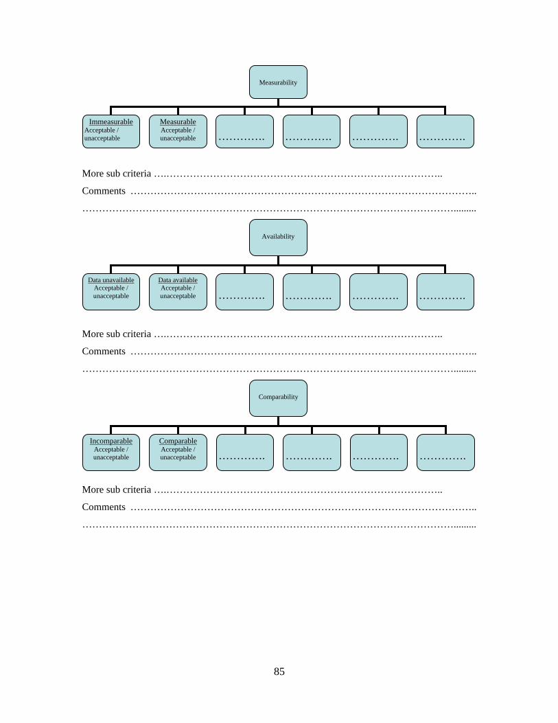
Measurability

Immeasurable Acceptable / unacceptable

Measurable Acceptable / unacceptable

………….

………….

………….

………….


Comments …………………………………………………………………………………………..

………………………………………………………………………………………………….........

Availability

Data unavailable Acceptable / unacceptable

Data available Acceptable / unacceptable

………….

………….

………….

………….


Comments …………………………………………………………………………………………..

………………………………………………………………………………………………….........

Comparability

Incomparable Acceptable / unacceptable

Comparable Acceptable / unacceptable

………….

………….

………….

………….


Comments …………………………………………………………………………………………..

………………………………………………………………………………………………….........

85

Importance

Useful for small groups

Acceptable / unacceptable

Useful for agencies


Useful for publicAcceptable / unacceptable

………….

………….

………….


Comments …………………………………………………………………………………………..

………………………………………………………………………………………………….........

4. Do you think that quantitative criteria listed above are acceptable and suitable to assess the

performance measure for freeway operation?

Yes ___

NO ___

If the answer is “No”, please suggest other criteria which should be added (fill out in blank

box) or omitted (circle).

Main criteria

Quantitative criteria

Time Acceptable / unacceptable

Cost Acceptable / unacceptable

Accuracy Acceptable / unacceptable

Reliability Acceptable / unacceptable

…………..

…………..

…………..

More criteria ………………………………………………………………………………..

Comments …………………………………………………………………………………………..

………………………………………………………………………………………………….........

86

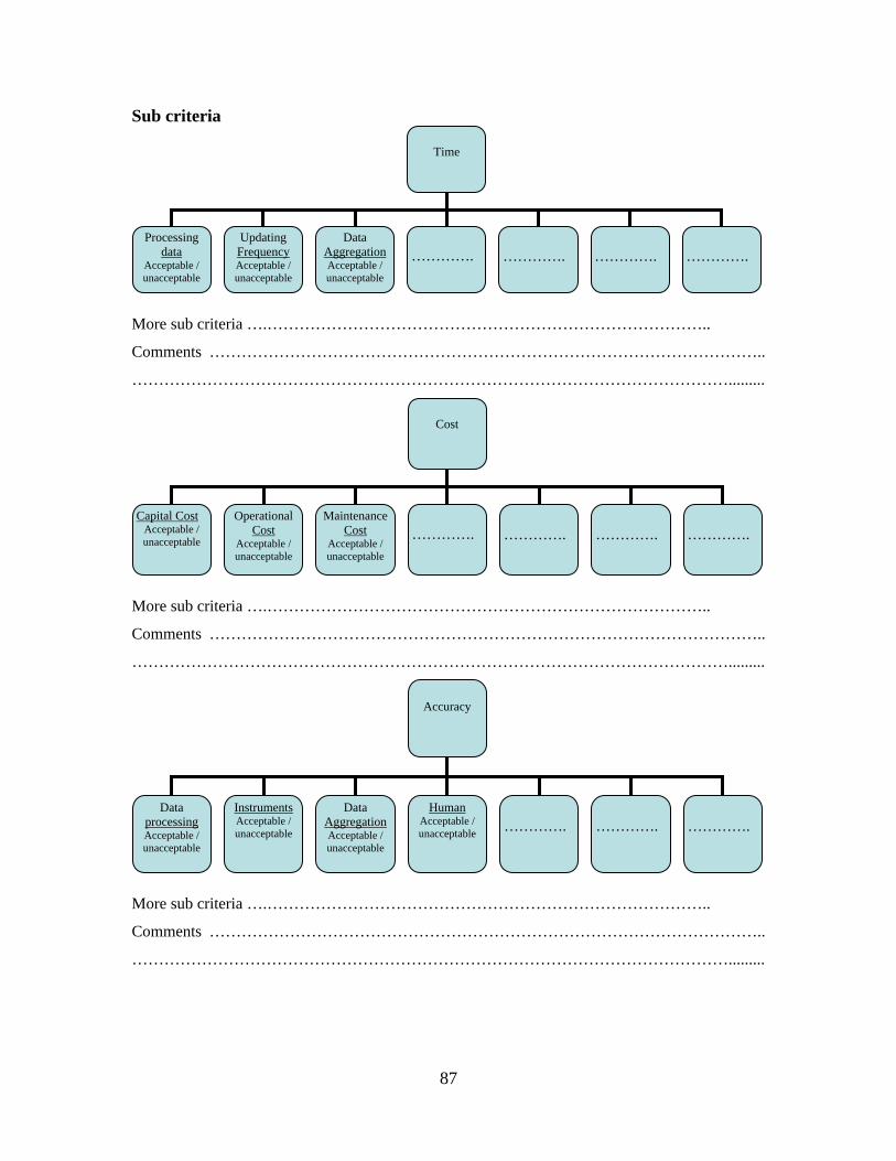
Sub criteria

Time

Processing data


Updating Frequency Acceptable / unacceptable

Data AggregationAcceptable / unacceptable

………….

………….

………….

………….


Comments …………………………………………………………………………………………..

………………………………………………………………………………………………….........

Cost

Capital Cost Acceptable / unacceptable

Operational Cost


Maintenance Cost


………….

………….

………….

………….


Comments …………………………………………………………………………………………..

………………………………………………………………………………………………….........

Accuracy

Data processing Acceptable / unacceptable

Instruments Acceptable / unacceptable

Data AggregationAcceptable / unacceptable

Human Acceptable / unacceptable

………….

………….

………….


Comments …………………………………………………………………………………………..

………………………………………………………………………………………………….........

87

88

Reliability

Equipment Acceptable / unacceptable

Communication Acceptable / unacceptable

Database Acceptable / unacceptable

………….

………….

………….

………….


Comments …………………………………………………………………………………………..

………………………………………………………………………………………………….........

Operations-Oriented Performance Measures for Freeway ... · Performing Organization Report No. ......

Documents

Transcript of Operations-Oriented Performance Measures for Freeway ... · Performing Organization Report No. ......