Operating Leverage,

Stock Market Cyclicality,

and the Cross-Section of Returns

Job Market Paper

François Gourio∗

December, 2004

Abstract

I use a putty-clay technology to explain several asset market facts. The key mechanismis as follows: a one percent increase in sales leads to a more-than-one percent increase inprofits, since labor costs don’t move one-for-one. This amplification is greater for plantswith low productivity for which the average profit margin (sales minus costs) is small. This“operating leverage” effect implies that low productivity plants benefit disproportionatelyfrom business cycle booms. These plants have thus higher systematic risk and higher averagereturns. This model can help explain the empirical findings of Fama and French (1992), andmore generally the sources of differences in market betas across firms. I obtain supportingevidence for the mechanism using firm- and industry-level data. The aggregate effect followsfrom trend growth: low-productivity plants outnumber high-productivity plants, making theaggregate stock market procyclical. I examine these aggregate implications and find thatthis model generates a volatile stock market return that predicts the business cycle.

∗Graduate Student, Department of Economics, University of Chicago. Email: francois@uchicago.edu. An

appendix is available on my web page, http://home.uchicago.edu/~francois. I thank the members of my

committee Fernando Alvarez, John Cochrane, and Anil Kashyap for their support and guidance, and I owe a

special debt to my chairman Lars Hansen for his advice and his encouragement. I received useful comments

from participants in several University of Chicago workshops, and from many people, especially Jeff Campbell,

Jonas Fisher, Boyan Jovanovic, Hanno Lustig, Pierre-Alexandre Noual, Monika Piazzesi, Adrien Verdelhan and

Pierre-Olivier Weill. All errors are mine. First draft of this project: June 2003.

1

1 Introduction

Ever since Fama and French (1992) showed that firms with high ratios of book value to market

value have high average returns, the economic interpretation of their finding has remained elusive.

Is book-to-market really an indicator of firm riskiness, if so why? In this paper, I consider the

asset pricing implications of a putty-clay technology: capital and labor are substitutable only ex-

ante (i.e., before capital investment is done). I show that under this technology, book-to-market

differences reflect differences in labor productivity, which result in different exposures to business

cycle risk. From a more general standpoint, the paper offers a theory of why different firms have

different expected returns by linking a firm’s financial risk with its real, observable attributes (or

characteristics). This technology-based interpretation of stock returns also has some interesting

aggregate implications: it is consistent with the fact that the return on the stock market is volatile

and forecasts the business cycle.

The key idea that I formalize is the “operating leverage”. Since costs move less than one-for-

one with output, an increase in output will result in a more than one-for-one increase in profits.

This amplification effect makes aggregate profits more cyclical than GDP; but the strength of

the amplification differs across firms. It follows that high productivity firms are less responsive

to aggregate shocks, i.e. less cyclical. This will be reflected in prices: the relative value of

productive firms falls in booms. The notion of productivity here is labor productivity. Having

a relatively productive plant is more valuable in recessions than in booms, because in recessions

aggregate productivity declines are larger than wages declines, making labor relatively expensive

as compared to capital. Conversely, in booms capital is scarce and labor is relatively cheap,

so that labor productivity is less advantageous. This explanation relies on the well-known fact

that wages don’t move as much as labor productivity over the business cycle. The theory is also

consistent with the Schumpeterian view that the least productive suffer more from recessions.

The logic of asset pricing based on macroeconomic risk implies that low productivity firms,

which are more procyclical, are more risky, and thus earn higher average returns. The model

rationalizes the correlation between book-to-market ratios and return by noting that productive

firms will tend to have a lower book-to-market, so that returns and book-to-market will be

positively correlated. The return differentials across assets are exactly justified by corresponding

differences in betas.

After developing the model and analyzing its asset pricing implications, I proceed to test this

theoretical explanation. I show that the book-to-market ratio is systematically related across firms

2

to productivity and operating leverage. I also show that the pattern of cyclicality of operating

income is close to the one predicted by the model: high book-to-market firms are more sensitive

to GDP changes and to labor compensation changes than low book-to-market firms, and these

estimates are of the order of magnitude predicted by the model. I also provide some supportive

patterns at the industry level.

When the relative value of productive firms falls, the value of the aggregate stock market

changes as well. How can a relative price effect change the aggregate value of the capital stock?

This is because trend growth in the economy makes installed capital on average less productive

than new investment, and thus the stock of capital resides predominantly with less productive

firms. Hence, when the value of low productivity firms increases relative to the value of high

productivity firms, the overall stock market rises. This revaluation mechanism is an alternative

to the widely used adjustment cost formulation (Cochrane 1991, Hall 2001). I show that the

mechanism can account relatively well for the business-cycle frequency movements in the stock

market: at the onset of recessions when capital is relatively abundant, the relative value of

productive units increases, which drives the stock market down. When expansions begin and

labor is relatively abundant, the low-productivity units become more valuable, which drives the

stock market up. The stock market return is a leading indicator of macroeconomic growth in the

model and in the data.

Organization

The next section is an overview of the main ideas and results of the paper. Section 3 presents

the model and Section 4 derives the asset pricing implications. Section 5 looks at firm- and

industry-level evidence, and Section 6 discusses macroeconomic evidence. Section 7 concludes.

2 Overview and main results

Although I develop a full dynamic stochastic general equilibrium model, the basic mecha-

nism is easily demonstrated in a static example. Consider the operating income of a firm with

fixed capital K and a standard constant-return-to-scale (CRS) production function F , facing

aggregate total factor productivity (TFP) A and wage w. Labor can be varied and profit is

π(K,A,w) = maxN≥0 {AF (K,N)− wN}. This profit is the value of the firm (its capital stock

and its technology) in a one-period world. The percentage increase in value in response to a

one-percent increase in aggregate TFP A is obtained using the envelope theorem, assuming for

3

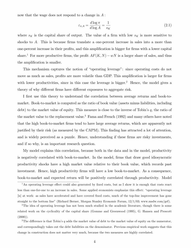
now that the wage does not respond to a change in A :

επ,A =d log π

d logA=1

sK(2.1)

where sK is the capital share of output. The value of a firm with low sK is more sensitive to

shocks to A. This is because firms translate a one-percent increase in sales into a more than

one-percent increase in their profits, and this amplification is bigger for firms with a lower capital

share.1 For more productive firms, the profit AF (K,N)−wN is a larger share of sales, and thus

the amplification is smaller.

This mechanism captures the notion of “operating leverage”: since operating costs do not

move as much as sales, profits are more volatile than GDP. This amplification is larger for firms

with lower productivities, since in this case the leverage is bigger.2 Hence, the model gives a

theory of why different firms have different exposures to aggregate risk.

I first use this theory to understand the correlation between average returns and book-to-

market. Book-to-market is computed as the ratio of book value (assets minus liabilities, including

debt) to the market value of equity. This measure is close to the inverse of Tobin’s q, the ratio of

the market value to the replacement value.3 Fama and French (1992) and many others have noted

that the high book-to-market firms tend to have large average returns, which are apparently not

justified by their risk (as measured by the CAPM). This finding has attracted a lot of attention,

and is widely perceived as a puzzle. Hence, understanding if these firms are risky investments,

and if so why, is an important research question.

My model explains this correlation, because both in the data and in the model, productivity

is negatively correlated with book-to-market. In the model, firms that draw good idiosyncratic

productivity shocks have a high market value relative to their book value, which records past

investment. Hence, high productivity firms will have a low book-to-market. As a consequence,

book-to-market and expected return will be positively correlated through productivity. Model

1An operating leverage effect could also generated by fixed costs, but as I show it is enough that costs react

less than one-for-one to an increase in sales. Some applied economists emphasize this effect: “operating leverage

[is] at work: as sales have accelerated and have covered fixed costs, much of the top-line improvement has gone

straight to the bottom line” (Richard Berner, Morgan Stanley Economic Forum, 12/1/03; www.msdw.com/gef).2The idea of operating leverage has not been much studied in the academic literature, though there is some

related work on the cyclicality of the capital share (Gomme and Greenwood (1995), G. Hansen and Prescott

(2000)).3The difference is that Tobin’s q adds the market value of debt to the market value of equity on the numerator,

and correspondingly takes out the debt liabilities on the denominator. Previous empirical work suggests that this

change in construction does not matter very much, because the two measures are highly correlated.

4

simulations reveal that the effect can be significant.

Next, I test empirically the proposed explanation for these cross-sectional facts. I examine

the model’s prediction that high book-to-market firms have a higher operating leverage, using

as a proxy for operating leverage the inverse capital share; this prediction holds in the data.

I then show that the cash flows (the operating income) of the high book-to-market firms is

more cyclical. More precisely, in the model, one can decompose changes in firm-level operating

income into changes in aggregate TFP and changes in the aggregate wage; denoting x the labor

productivity of the firm, we have:

∆OIt(x) =Atx

Atx− wt1

sK (x)

∆At+−wt

Atx− wt1− 1

sK (x)

∆wt, (2.2)

where ∆OIt is the % change in operating income, ∆At the % change in aggregate TFP, and ∆wt

is the % change in the aggregate wage, and sK(x) is the capital share of a firm with productivity

x. Equation (2.2) makes the following predictions: (i) if we take the average capital share to

be 1/3, the coefficient on TFP growth should be on average 1/(1/3)=3; (ii) high book-to-market

firms, which have low productivity x, should have a higher coefficient in front of TFP growth; (iii)

and inversely, the coefficient on wage growth should be decreasing in book-to-market. I run this

regression for each portfolio (i.e. groups of firms sorted by book-to-market; with GDP instead

of TFP, see the details in Section 5). Perhaps surprisingly in light of the previous literature,

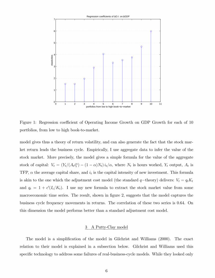
the estimates actually give some support to the model: a 1% increase in GDP leads to a 3%

increase of operating income for the whole sample of firms, but the effect differs across firms. The

operating income of the the high book-to-market firms rises by 6% whereas it rises by only 1.5%

for the low book-to-market firms. Finally, the coefficient on wage growth, though not monotonic,

is more negative for higher book-to-market portfolios. These results are illustrated in figure 1

below, which plots the coefficient estimates on GDP growth, for each portfolio. Hence, the model

captures an economic reason why high book-to-market firms are more risky.

Finally, I examine the aggregate, time-series implications of the model. Low-productivity

plants outnumber high-productivity plants: trend growth in the economy makes installed cap-

ital on average less productive than new investment, and thus the stock of capital resides pre-

dominantly with less productive firms. (To put it another way, low-productivity here means a

productivity lower than marginal plants, which are the ones we are building today - the only

margin of action possible in this simple setup.) Hence, when the value of low productivity firms

increases relative to the value of high productivity firms, the overall stock market rises. The

5

0 1 2 3 4 5 6 7 8 9 10 110

1

2

3

4

5

6

7

portfolios from low to high book−to−market

ela

stic

ities

Regression coefficients of ∆O.I. on ∆GDP

Figure 1: Regression coefficient of Operating Income Growth on GDP Growth for each of 10

portfolios, from low to high book-to-market.

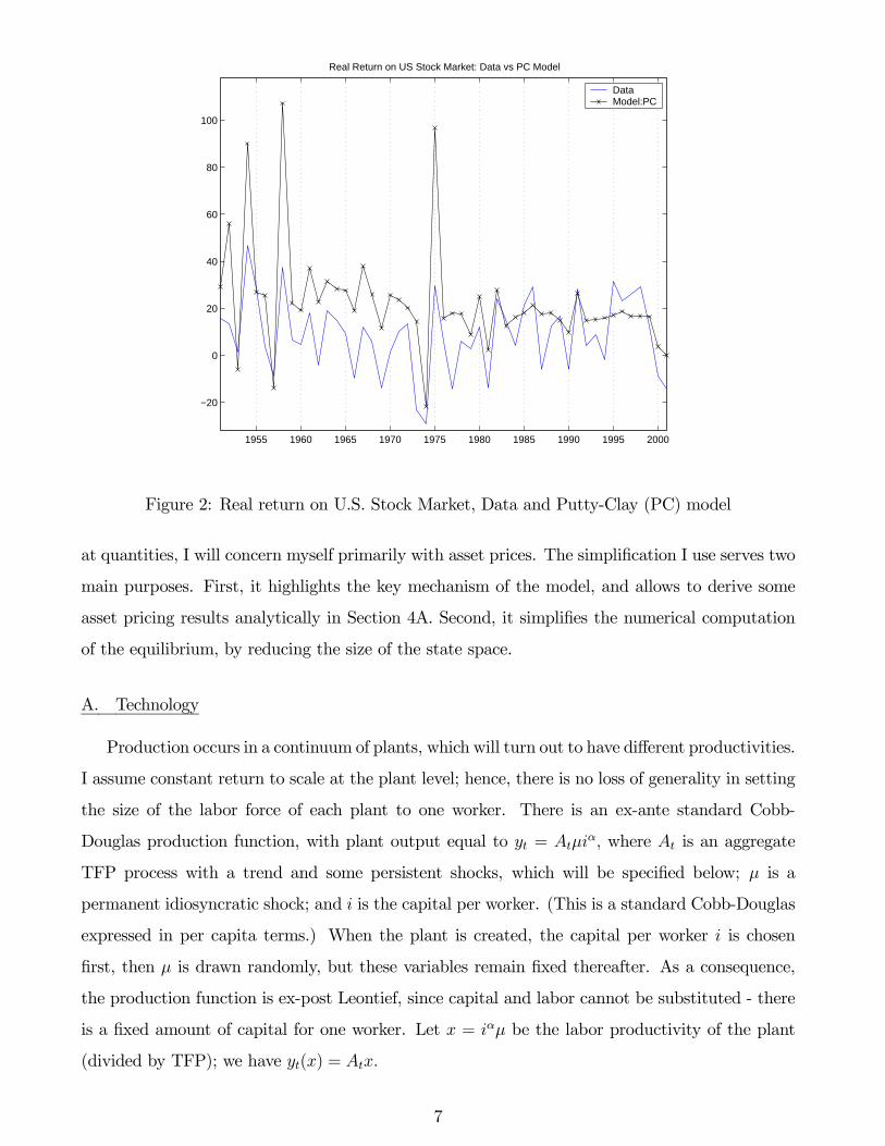
model gives thus a theory of return volatility, and can also generate the fact that the stock mar-

ket return leads the business cycle. Empirically, I use aggregate data to infer the value of the

stock market. More precisely, the model gives a simple formula for the value of the aggregate

stock of capital: Vt = (Yt/(Atiαt )− (1− α)Nt) it/α, where Nt is hours worked, Yt output, At is

TFP, α the average capital share, and it is the capital intensity of new investment. This formula

is akin to the one which the adjustment cost model (the standard q−theory) delivers: Vt = qtKt

and qt = 1 + c (It/Kt). I use my new formula to extract the stock market value from some

macroeconomic time series. The result, shown in figure 2, suggests that the model captures the

business cycle frequency movements in returns. The correlation of these two series is 0.64. On

this dimension the model performs better than a standard adjustment cost model.

3 A Putty-Clay model

The model is a simplification of the model in Gilchrist and Williams (2000). The exact

relation to their model is explained in a subsection below. Gilchrist and Williams used this

specific technology to address some failures of real-business-cycle models. While they looked only

6

1955 1960 1965 1970 1975 1980 1985 1990 1995 2000

−20

0

20

40

60

80

100

Real Return on US Stock Market: Data vs PC Model

DataModel:PC

Figure 2: Real return on U.S. Stock Market, Data and Putty-Clay (PC) model

at quantities, I will concern myself primarily with asset prices. The simplification I use serves two

main purposes. First, it highlights the key mechanism of the model, and allows to derive some

asset pricing results analytically in Section 4A. Second, it simplifies the numerical computation

of the equilibrium, by reducing the size of the state space.

A. Technology

Production occurs in a continuum of plants, which will turn out to have different productivities.

I assume constant return to scale at the plant level; hence, there is no loss of generality in setting

the size of the labor force of each plant to one worker. There is an ex-ante standard Cobb-

Douglas production function, with plant output equal to yt = Atµiα, where At is an aggregate

TFP process with a trend and some persistent shocks, which will be specified below; µ is a

permanent idiosyncratic shock; and i is the capital per worker. (This is a standard Cobb-Douglas

expressed in per capita terms.) When the plant is created, the capital per worker i is chosen

first, then µ is drawn randomly, but these variables remain fixed thereafter. As a consequence,

the production function is ex-post Leontief, since capital and labor cannot be substituted - there

is a fixed amount of capital for one worker. Let x = iαµ be the labor productivity of the plant

(divided by TFP); we have yt(x) = Atx.

7

More precisely, new plants are built each period; but in contrast to the standard neoclassical

model where new investment is simply a matter of choosing the quantity of capital to build,

this model introduces an extra choice, the capital intensity of the new investment. Each period,

each new plant decides once and for all its capital per worker, or capital intensity, it. (Since we

normalize the size to be one worker, it is also the total investment required to build the plant.)

Once this choice is made, each plant draws a permanent idiosyncratic productivity shock µ with

c.d.f. H(.) and mean Eµ = 1 =∞0tdH(t)dt. This yields a plant of productivity4 iαt µ. The

average productivity of new plants built at time t is thus xt = Eµ (iαt µ) = iαt . Investment is

irreversible. Moreover, it is not possible to increase ex-post the capital of a given plant: hence,

one cannot take advantage of a good draw of µ to increase the size of the plant. Rather, an

increase in investment must take the form of new plants creation, which will draw their own new

µ.5

Let ht be the number of new plants built at time t. These plants come into operation in

the following period. Moreover, plants die at rate δ: hence, depreciation is a matter of plants

disappearing, not a shrinkage of capital within each plant. Hence, we obtain the following law of

motion for the measure Gt of plants with productivity less than x:

Gt+1(x) = (1− δ)Gt(x) + htHx

xt, (3.1)

i.e. plants of productivity less than x at time t + 1 are plants of productivity less than x at

time t that did not depreciate, plus new plants: these were designed in quantity ht with average

productivity xt but H (x/xt) happened to draw µ ≤ x/xt and end up with a productivity µxt, lessthan x. In the end, the distribution of productivity Gt will exhibit dispersion for three reasons:

first, the idiosyncratic shock µ; second, the trend imparted by growth to the average productivity

xt: capital deepening (or embodied progress, see footnote 4) makes recently built units more

productive; and third, stochastic variations around the trend in xt. Since the heterogeneity in4It is natural in this setup to introduce embodied technology: the productivity of new plants is then iαt µBt where

logBt = µbt. This does not prove very useful for my asset pricing work, so for simplicity I withdraw this source

of growth and business cycles. See Christiano and Fisher (2003), Fisher (2002), Gilchrist and Williams (2000)

and Greenwood, Hercowitz and Krusell (2001) for evaluations of the business cycle consequences of embodied

technology shocks.5As can be deducted from the results of section 3, it is possible to obtain similar results without the productivity

shock µ. However, in this case: (1) cohort effects will explain all of productivity variation, and of book-to-market

variation, and (2) the cross-sectional distribution over productivity is degenerate. To avoid these weaknesses, and

since adding µ leads to no loss in tractability, I consider µ to be important. (See the discussion on the empirical

evidence for µ in the text.)

8

productivity is central to the model, it is noteworthy that a large recent literature in industrial

organization has measured large differentials of productivity between establishments, even within

4-digit industries (Bartelsman and Doms (2000)). As an example, Syverson (2004) computes that

within such an industry, a plant in the 25th percentile of labor productivity is nearly twice as

productive as a plant in the 75th percentile.

There are no adjustment costs along the extensive margin, i.e. the number of new plants

opening: hence, a free-entry condition determines the quantity ht of new plants. The key variable

in the model is it, the capital intensity of new investment, so let us pause to understand how

it is chosen. This capital intensity choice is dictated by the following trade-off: a higher capital

intensity it requires a higher initial investment, but decreases future costs per unit of output -

that is, future labor costs will absorb a lower share of output. Hence, depending on expected

future interest rates, TFP and wages, firm will choose the cost-minimizing it. Since plants are

identical ex-ante, and make the same forecasts regarding future wages, TFP and interest rates,

they have no reason to choose different it, and thus all end up with the same choice. Of course,

because of the idiosyncratic shock µ, some plants get a higher productivity, and some a lower

productivity, than xt = iαt .

Aggregating across plants yields total output Yt and total hours worked Nt :

Yt =∞

0

Atx dGt(x) (3.2)

Nt =∞

0

dGt(x). (3.3)

Since Gt(.), the quantity of capital of each productivity, is predetermined, output is predeter-

mined, up to the TFP shock to At, and so are hours. Within the period, labor demand is fully

inelastic. As usual, I assume that the labor market clears, with the wage moving to induce supply

to adjust to the fixed demand.

Define Yt =∞0xdGt(x) = Yt/At the total productive capacity of the economy, not taking

into account TFP. Using the law of motion (3.1) of the distribution Gt(.), we can find the law of

motion for Yt :

Yt =YtAt=

∞

0

xdGt(x)

=∞

0

x (1− δ)dGt−1(x) + ht−1dHx

xt−1

= (1− δ)∞

0

xdGt−1(x) + ht−1∞

0

xdHx

xt−1

9

= (1− δ)Yt−1 + ht−1xt−1, (3.4)

where the last line used that Eµ = ∞0tdH(t) = 1. Similarly for Nt:

Nt =∞

0

dGt(x)

=∞

0

(1− δ)dGt−1(x) + ht−1dHx

xt−1

= (1− δ)∞

0

dGt−1(x) + ht−1∞

0

dHx

xt−1= (1− δ)Nt−1 + ht−1, (3.5)

where the last line uses that dH(.) is a density.

The distribution Gt(.) disappears from our problem since all its effects are summarized in the

state variables Yt and Nt: these two variables together tell us the total production capacity and

the total number of plants (Here and everywhere, the number of plants is the number of their

employees). This is a payoff for the simplification I make to the setup of Gilchrist and Williams.

B. Preferences, Resource Constraint, Planner Problem

Themodel is closed with a representative household who has preferences E0 t≥0 βtU (ct, 1−Nt) .

The resource constraint is ct + htit ≤ Yt. Note that htit is the aggregate investment: there are htnew plants with it units of capital per new job. Finally, growth occurs through growth in TFP

At, i.e., ways of using existing plants more efficiently. I assume a deterministic trend, and AR(1)

deviations from the trend:

logAt = µat+ εat

εat = ρaεat−1 + u

at ,

with the innovation uat iid N(0,σ2a).

In the end, the model can be solved using the following planning problem:

max{ct,it,ht,Yt+1,Nt+1}∞

t=0

E∞

t=0

βtU(ct, 1−Nt)

s.t. : ct + itht ≤ AtYt

Yt+1 = (1− δ)Yt + iαt ht

Nt+1 = (1− δ)Nt + ht

Y0, N0 given

10

First-order conditions are easily obtained (see appendix 2). The numerical techniques used to

find the equilibrium and to compute asset prices are discussed in appendix 4.

Comparison with Gilchrist and Williams and Business Cycle Implications

In their model, Gilchrist and Williams (2000) consider the possible decision to shut down a

plant, i.e. not hire a worker, if it becomes unprofitable, whereas I do not take this into account.

As a result, the mechanisms I emphasize do not rely on varying utilization.6 On the other

hand, one might worry that some plants are operating despite being unprofitable in my version.

(firms that draw a very low µwill still operate despite making losses.) In some cases, there

are no such plants: my simplification is exactly true. In some other cases, it will be a good

approximation to the Gilchrist and Williams model where plants choose to open or close each

period.7 Alternatively, my model can be viewed as building on the opposite assumption than

Gilchrist andWilliams: no closures are allowed, whereas in their model switching between opening

and closing is instantaneous and costless. As a result from the similarity between the models,

business-cycle results close to those of Gilchrist and Williams (2000) are obtained in this model.

These findings are documented in appendix 3, where I also show that the number of unprofitable

plants in my model is small for the parameter values I choose.

4 Asset Pricing

This section first gives some analytical results that develop the intuition given in the intro-

duction, then offers some numerical simulations.

A. Analytical results

Since each plant is a particular capital good, characterized by its labor productivity, I start by

pricing each one separately. I then obtain the aggregate implications - the return on a diversified

portfolio of plants - by summing over the existing stock of plants. A plant of productivity x will

yield cash-flows Dt(x) = Atx− wt where wt is the wage and At is TFP. The ex-dividend price is6In the model with variable utilization, because units are kept indefinitely and switched on/off at no cost, the

value of a plant has an important option component to it. (Indeed, the price as a function of productivity is

convex, whereas it will be linear here.) I do not study these effects, which may be interesting.7The simplification is the exact solution if the technology growth rates are zero, the depreciation rate is large

enough, the aggregate shocks have a small variance, and if the distribution h has a narrow support around its unit

mean; the simplification is a good approximation for not-too-big changes in the parameters from these values.

11

the present-value of cash-flows, discounted using a stochastic discount factor8 mt,t+j:

Pt(x) = Etj≥1mt,t+j (1− δ)j−1Dt+j(x)

Pt(x) = x · Etj≥1mt,t+j (1− δ)j−1At+j − Et

j≥1mt,t+j (1− δ)j−1wt+j

Pt(x) = xv1t − v2t, (4.1)

where the last equation defines v1t and v2t as the present discounted values of TFP and the wage.

This formula reveals that plants with different productivities x will have different sensitivities

to aggregate shocks: these prices are all driven by the same aggregate variables v1t and v2t, but

plants with different x will react differently to changes in v1t and v2t. I show below that v1t and

v2t can both be expressed solely as a function of the variable it, the capital intensity of new plants.

In the terminology of asset pricing, it is thus an asset pricing factor.9

Comparison to other technologies and related literature

Before developing in more detail the implications of (4.1), it may be useful to see which assump-

tions drive this representation, and how it relates to other possible technological assumptions (but

some readers may prefer to skip this section on first reading and proceed directly to the analysis

of my model). First, notice that in a model with fixed capital, i.e. kt+j = k(1− δ)j−1, and fixed

idiosyncratic shock x, but a fully adjustable capital-labor ratio (i.e., labor) in a Cobb-Douglas

production function, the price would be

Pt(x, k) = Etj≥1mt,t+j max

nt+jAt+jxk

αt+jn

1−αt+j − wt+jnt+j

= Etj≥1mt,t+jζk(1− δ)j−1 (At+jx)

1α w

α−1α

t+j ,

where ζ is a constant; we can write Pt(x, k) = x1/αvt and firms with different x would have

the same sensitivities to aggregate shocks. Hence, the representation (4.1) breaks down with a

simple Cobb-Douglas production function. However, this will not be true under more general

8A stochastic discount factor is a variable that adjusts payoffs for the times and states in which the payoffs are

paid, to reflect impatience and risk-aversion. In complete markets, the stochastic discount factor equals the ratio

of the state-contingent Arrow-Debreu price to the probability of the state. In our case, the stochastic discount

factor will also equal the ratio of marginal utilities of consumption: mt,t+j = βjUc(ct+j , 1−Nt+j)/Uc(ct, 1−Nt).9This result breaks down when embodied-technology shocks are added; in this case, v1t and v2t are two non-

redundant factors.

12

CRS production functions. Thus, my result and central argument does not require putty-clay,

and it seems that the argument will hold with a low, positive substitutability between capital and

labor. The putty-clay formulation however is simpler and delivers sharper results.10 The model

features thus constant capital and labor at the plant level. While the full structure of the model

will be exploited for the aggregate results, it seems that the cross-sectional results do not rely on

the putty-clay assumption per se: the fact that labor is fixed in particular is not important. What

is key is that the cost of labor moves less than the average productivity in response to a shock.

More generally, one could envision having fixed as well as variable costs: what really matters is

that costs do not change much over time (for a marginal shock). The fixed capital assumption is

more important, but I conjecture that similar results would hold under strong adjustment costs.

(The literature, up to now, relies on strong adjustment costs to prevent the reallocation of capital

towards the most efficient units.)

Adjustment costs

In my model, firms cannot add capital by extending productive plants: they must set up

new plants which will draw new productivity shocks; hence it is not really possible to take

advantage of a good productivity. This is a strong form of adjustment costs - but on the other

hand, there are no adjustment costs along the new plants margin. To go beyond this fixed capital

formulation, the natural idea is to introduce adjustment costs, which will relate book-to—market to

risk through investment patterns. First, note that heterogeneity in capital, without heterogeneity

in productivity, will not help, since in this case again all firms’ values move in step. To see this,

write the Bellman equation

V (K, z) = maxI

Kh(z)− Iφ I

K+ Ez /z (m(z, z )V (K , z )) ,

where z is an aggregate Markov state; K is capital; m is a stochastic discount factor; and the profit

function Kh(z) is linear in capital under constant returns and perfect competition. Hayashi’s

theorem (1982) implies that we can write V (K, z) = Kg(z), and thus d log V (K, z)/d log z is

independent of K. An obvious remedy is to add idiosyncratic shocks, and write the problem (still

assuming a fixed x) as

V (K, z, x) = maxI

Kh(z, x)− Iφ I

K+ Ez /z (m(z, z )V (K , z , x)) .

Again V (K, z, x) = Kg(z, x), but now unless g is multiplicatively separable, i.e. unless g can be

written as g(z, x) = g1(z)g2(x), firms with different productivities will have different exposures10Note that the aggregate effects that will be derived below rely on the whole structure of the model and are

less robust to model extensions.

13

to aggregate states z. This model can potentially generate the book-to-market effect: high pro-

ductivity firms have higher price and lower book-to-market, and may be more risky. A variant of

this model, in partial equilibrium, has been studied by Zhang (2004). One hindrance to studying

this model in general equilibrium is a “curse of dimensionality” that arises since it is necessary

to keep track of the whole cross-sectional distribution. (Also, the limited success of the firm-level

q-theory embedded in this model may have discouraged researchers.) Kogan, Gomes and Zhang

(2003) and Gala (2004) have studied related models with adjustment costs where additional as-

sumptions allow to break the curse of dimensionality and to justify the size effect (the tendency

for smaller firms to have larger average returns than a CAPM risk adjustment predicts). Carlson

et al. (2004) emphasized option values, and Cooper (2003) studied a model with fixed costs to

adjusting the capital stock.

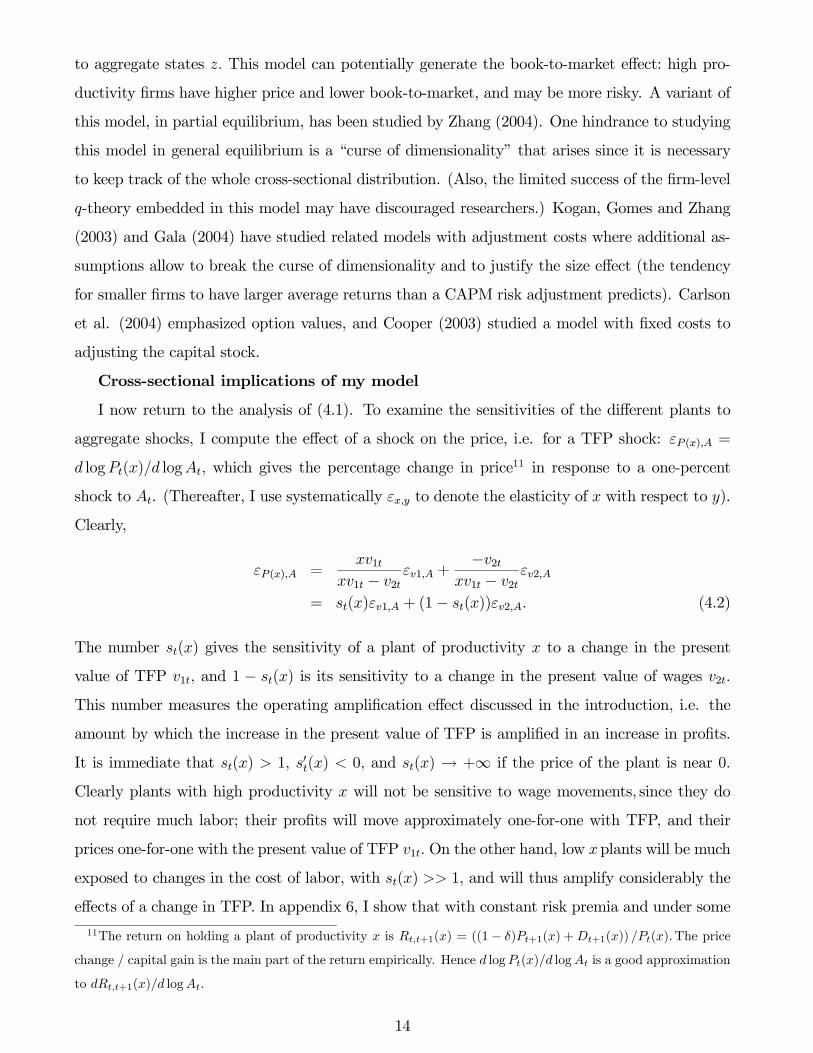
Cross-sectional implications of my model

I now return to the analysis of (4.1). To examine the sensitivities of the different plants to

aggregate shocks, I compute the effect of a shock on the price, i.e. for a TFP shock: εP (x),A =

d logPt(x)/d logAt, which gives the percentage change in price11 in response to a one-percent

shock to At. (Thereafter, I use systematically εx,y to denote the elasticity of x with respect to y).

Clearly,

εP (x),A =xv1t

xv1t − v2t εv1,A +−v2t

xv1t − v2t εv2,A= st(x)εv1,A + (1− st(x))εv2,A. (4.2)

The number st(x) gives the sensitivity of a plant of productivity x to a change in the present

value of TFP v1t, and 1 − st(x) is its sensitivity to a change in the present value of wages v2t.This number measures the operating amplification effect discussed in the introduction, i.e. the

amount by which the increase in the present value of TFP is amplified in an increase in profits.

It is immediate that st(x) > 1, st(x) < 0, and st(x) → +∞ if the price of the plant is near 0.

Clearly plants with high productivity x will not be sensitive to wage movements, since they do

not require much labor; their profits will move approximately one-for-one with TFP, and their

prices one-for-one with the present value of TFP v1t. On the other hand, low xplants will be much

exposed to changes in the cost of labor, with st(x) >> 1, and will thus amplify considerably the

effects of a change in TFP. In appendix 6, I show that with constant risk premia and under some

11The return on holding a plant of productivity x is Rt,t+1(x) = ((1− δ)Pt+1(x) +Dt+1(x)) /Pt(x).The price

change / capital gain is the main part of the return empirically. Hence d logPt(x)/d logAt is a good approximation

to dRt,t+1(x)/d logAt.

14

simplifying assumptions, st(x) Atx/(Atx−wt) is the inverse of the capital share: we obtain thusagain approximately the measure of operating leverage presented in the static model discussed in

the overview section. (In Section 5, I will use this as an empirical measure of operating leverage.)

To obtain a more precise characterization of how the prices of plants of different productivities

react to aggregate shocks, one needs to use the two conditions that govern the creation of new

plants.12

• First, when building a new plant, each investor chooses the capital intensity it of his plant,to obtain the highest expected value of the plant, net of the investment cost; the expectation

is taken over µ, which is unknown at the time of investment:

it ∈ argmaxi{EµPt (iαµ)− i}

⇒ it ∈ argmaxi{iαv1t − v2t − i} ,

where the second line uses our expression (4.1) for the price of a project, the linearity in x

of the price, and the fact that Eµµ = 1. The first-order condition yields

v1t =i1−αt

α. (4.3)

• Next, we use the free-entry condition that the (expected) price of the plants that are builttoday equals their cost:

EµPt (iαt µ) = it

iαt v1t − v2t = it.

To put it another way, Tobin’s q is one for the plants which we are adding today to our capital

stock, since there are no adjustment costs along this margin. Combining this equation with

(4.3) yields

v2t =1− α

αit. (4.4)

These relations agree with intuition. According to (4.3), when future discounted TFP v1t is

high, plants choose a high capital intensity it, using capital deepening to take advantage of the

future good productivity. Similarly, according to (4.4), when the future discounted wages v2t are

high, plants economize on labor by increasing the capital intensity it.

12These conditions can be found directly by solving the social planner problem mentioned above (see appendix

2). Here I justify these conditions using a market interpretation.

15

Taking into account these two conditions simplifies our computation of the price sensitivity

(4.2):

εP (x),A = st(x)εv1,A + (1− st(x))εv2,A= st(x)(1− α)εi,A + (1− st(x))εi,A= (1− αst(x)) εi,A. (4.5)

Hence we see that plants with different x react proportionately to εi,A, but the sign and

magnitude of the response depends on x. Simple algebra using (4.3) and (4.4) allows us to rewrite

(4.5) as the:

• Result 1: The sensitivity of the price of a plant with productivity x to a TFP shock is

εP (x),A = (1− αst(x)) εi,A =1− α

α

x− xtPt(x)

εi,A (4.6)

where xt = iαt is the average productivity of plants built today (today’s “optimal produc-

tivity”), εi,A is the elasticity of it with respect to At, and st(x) = xv1t/(xv1t − v2t).

In response to a shock to TFP, the price of plants with a productivity lower than xt goes

up if it goes down. The reason for this relation is clear: when the capital intensity it of new

investment falls, it reflects that low productivity firms becomes relatively more efficient. (This is

because investors that have a choice, those who are building new plants, prefer a lower capital

intensity and thus a lower productivity - their choice is the only margin of adjustment of the

economy, and thus reveals us the value of the existing stock.) As a consequence, the price of

the low-productivity plants goes up by more than the high-productivity plants if and only if

εi,A < 0 (since ∂εP (x),A/∂x = −αst(x)(x)εi,A from (4.5), and st(x) < 0). Note that in this case,

the present value of TFP and the wage fall when a TFP shock hits the economy: though TFP is

higher, interest rates move up even more.13

Of course, the capital intensity of new investment i is itself an endogenous variable, chosen to

maximize profits: it balances higher expected discounted wages with higher expected discounted

TFP (as explained in the discussion of 4.3-4.4). An increase in i signals that labor is relatively

expensive, since new investment takes the form of capital-intensive plants that economize on

13This suggests that I will obtain this result for a low IES in my simulation, which is actually true. I also require

a high substitability of labor and a nonpermanent shock to get this key condition ∂i/∂A numerically. Of course,

other mechanisms, such as rigid wages, or labor market frictions, could explain why the present value of wages

moves less than the present value of TFP.

16

labor. On the other hand, a low i signals that labor is relatively cheap. And cheap labor makes

low productivity plants relatively more attractive: variations in the value of high-productivity vs.

low-productivity plants can be traced down to variations in the relative value of labor.

I will concentrate my studies to the case where εi,A < 0 : the optimal capital intensity of new

investment falls in booms; this requires some explanations. First, note that this condition does

not hold for all parameter values in the model,14 but I will choose a parametrization such that

it does. Why am I drawn to consider this condition? Since εv2,A = εi,A and εv1,A = (1 − α)εi,A,

it is equivalent to having εv1,A > εv2,A i.e. the present-value of TFP changes by more than the

present-value of wages. I believe this is the empirically relevant case for business-cycle movements,

since the wage is not strongly procyclical: the value of production moves by more than the cost

of labor. Another way to see it is to interpret εi,A < 0 as follows: in booms, the capital intensity

of new investment falls, i.e. we try to economize on capital by using more labor, which reflects

that labor is relatively cheap. It may seem surprising at first that labor is relatively cheap in

booms; however, this makes perfect sense: since the wage does not move as much as average labor

productivity, using labor is more attractive in booms than in recessions.15 In Section 6, I show

that an empirical measure of i is indeed strongly countercyclical.

With εi,A < 0, we obtain the intuition given in the introduction: plants with a low operating

income Atx − wt, i.e. low-productivity plants, are more sensitive to aggregate shocks: εP (x),A isdecreasing in x. As in the introduction, this results from the relative smoothness of wages. The

Consumption Asset Pricing Model that is embedded in this model then implies that low x plants

have higher returns. Note two extra predictions from (4.6): the very high x could have a negative

risk premium, and the pattern of volatility should be U- shaped, with low x and very high x

having higher volatilities.

Taking a step back, the idea that less productive firms suffer more from recessions is intu-

itive and empirically supported, and it has a long history, associated with Schumpeter (1942).

Caballero and Hammour (1994) develop the idea that recessions “clean” the economy of the less

productive units. Baily, Bartelsman and Haltiwanger (2001) provide evidence that less produc-

tive plants are more cyclical. Bresnahan and Raff (1991) discuss the vivid example of car plants

during the Great Depression.

14Indeed, there is a tendency for the opposite to occur, since we know that the standard response to a permanent

increase in TFP is capital deepening, i.e. an increase in the capital-labor ratio.15Another way to state it, is to look at the complementary factor: capital is scarcer in booms and almost

marginally useless in recessions.

17

Relation with Book-to-market and Tobin’s q

I will apply the model to book-to-market sorted portfolios. This is because book-to-market

will be strongly negatively correlated with productivity in this model. Book-to-market is defined

as it−j/Pt(x)where it−j is the capital intensity chosen at the time of investment, which is the

investment cost, and x = iαt−jµ is the productivity obtained as a result. Plants that draw good

idiosyncratic shocks µ will have a higher productivity x and thus a higher value Pt(x). (Remember

that Pt(x) = v1tx − v2t is always increasing in x.) Since this good idiosyncratic shock is notreflected in their book value it−j, they will have a low book-to-market ratio.

There is another reason why book-to-market will negatively correlate with productivity, which

has to do with the age of the plant. Since productivity, up to TFP, is fixed once and for all in

each plant at the construction stage, whereas productivity increases over time in the economy

(due to capital-deepening (and embodied technology, if any)), a plant’s price will on average fall

over time. This occurs because wages grow faster than the plant’s productivity. Since the book

value is fixed, and the price declines over time, old firms will have a higher book-to-market, in

as much as their price fell because they became less productive than the most recent ones. This

gives another source of negative correlation between productivity and book-to-market. Because

of stochastic fluctuations around the balanced growth path, all these correlations are imperfect.

It is interesting to note that these correlations are also found in the data. Using the LRD

plant-level manufacturing data set, Dwyer (2001) found that plants with low TFP or low labor

productivity have high book-to-market. Jovanovic and Rousseau (2002) found that old firms have

higher book-to-market, where age is measured as time being listed.

Notice that my definition draws a distinction between Tobin’s q and the book-to-market ratio:

the book-to-market ratio measures the ratio of price to the investment cost, not the replacement

cost.16 Still, it will prove instructive to compute Tobin’s average q for any plant of productivity

x as the ratio of the market value Pt(x) to the replacement cost.17 The replacement cost is

16A firm that draws a good productivity shock will be identical ex-post to a firm that chose a high capital

intensity. Hence, the replacement cost counts the efficiency units of capital to be installed to replicate this firm,

and it will be higher than the book value. Perfect and Wiles (1994) perform comparisons of various measures of

Tobin’s q and find some differences; in particular, the measure that uses the book value, as opposed to an estimate

of the replacement value, on the denominator, leads to different results in some regressions often used in corporate

finance. It seems hard, however, to generalize from their results.17Note that the book value measure that Fama and French use is the book value of stockholder’s equity, roughly

assets minus liabilities. Since liabilities include the debt book value (not market value) this could create a

measurement problem. (Debt market value is hard to find.) Previous empirical work however suggests that debt

18

80 85 90 95 100 105 110 115 1200.8

0.85

0.9

0.95

1

1.05

1.1

Productivity (in % of today optimal productivity)

Tob

in Q

Figure 3: Tobin’s q as a function of productivity. Tobin’s q is one for the productivity of capital

built today.

c(x) = x1/α since to obtain a plant of productivity x, one needs to put up i = x1/α units of

capital. Thus,

qt(x) =Pt(x)

c(x)=v1tx− v2tx1α

.

This function qt satisfies qt(xt) = 1, qt(xt) = 0, and qt(x) ≤ 1 for all x ≥ 0 : Tobin’s q is belowone for all productivities, except the one which is optimal today. The irreversibility constraint

binds for all productivities except the one that is optimal today; hence the market value falls

below the replacement cost for all productivities but x = xt, as shown in figure 3.

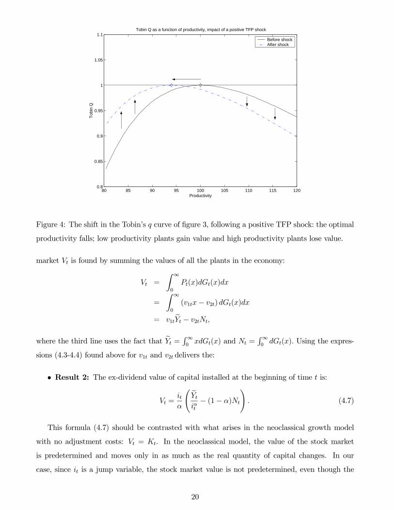
The effect of a TFP shock is depicted in figure 4: because the optimal productivity -the

point where q = 1- falls, under the maintained assumption that εi,A < 0, the curve shifts to

the left; hence, the q of the low-productivity plants rises whereas the q of the high-productivity

falls: this corresponds to a rise in the price of low-productivity plants, and a fall in the price of

high-productivity plants, which is an illustration of result 1.

Aggregate Implications: aggregate consequences from the relative price effect

I now turn to the aggregate implications. The (ex-dividend) value of the aggregate stock

does not explain the correlation between returns and book-to-market.

19

80 85 90 95 100 105 110 115 1200.8

0.85

0.9

0.95

1

1.05

1.1Tobin Q as a function of productivity, impact of a positive TFP shock

Productivity

Tob

in Q

Before shockAfter shock

Figure 4: The shift in the Tobin’s q curve of figure 3, following a positive TFP shock: the optimal

productivity falls; low productivity plants gain value and high productivity plants lose value.

market Vt is found by summing the values of all the plants in the economy:

Vt =∞

0

Pt(x)dGt(x)dx

=∞

0

(v1tx− v2t) dGt(x)dx

= v1tYt − v2tNt,

where the third line uses the fact that Yt =∞0xdGt(x) and Nt =

∞0dGt(x). Using the expres-

sions (4.3-4.4) found above for v1t and v2t delivers the:

• Result 2: The ex-dividend value of capital installed at the beginning of time t is:

Vt =itα

Ytiαt− (1− α)Nt . (4.7)

This formula (4.7) should be contrasted with what arises in the neoclassical growth model

with no adjustment costs: Vt = Kt. In the neoclassical model, the value of the stock market

is predetermined and moves only in as much as the real quantity of capital changes. In our

case, since it is a jump variable, the stock market value is not predetermined, even though the

20

quantities of capital - the Gt(x) - are. Hence, this theory generates some volatility in the price of

capital, even though there are no adjustment costs to the creation of new plants.18

Since Yt and Nt are predetermined (state) variables, any instantaneous impact on the value

of capital must go through it, the only jump (control) variable in (4.7). In appendix, a simple

evaluation of derivatives yields the following:

• Result 3: around the nonstochastic steady-state, Vt falls when it rises if and only if thereis trend growth.

We already know that the price of individual plants will move only if it changes (see equation

(4.6)). This result shows that to obtain a change in the aggregate price, one needs on top that there

is trend growth. The intuition is clear: with trend growth, there are much more low-productivity

plants than high-productivity: in the formula (4.6), most x are below the current optimal one

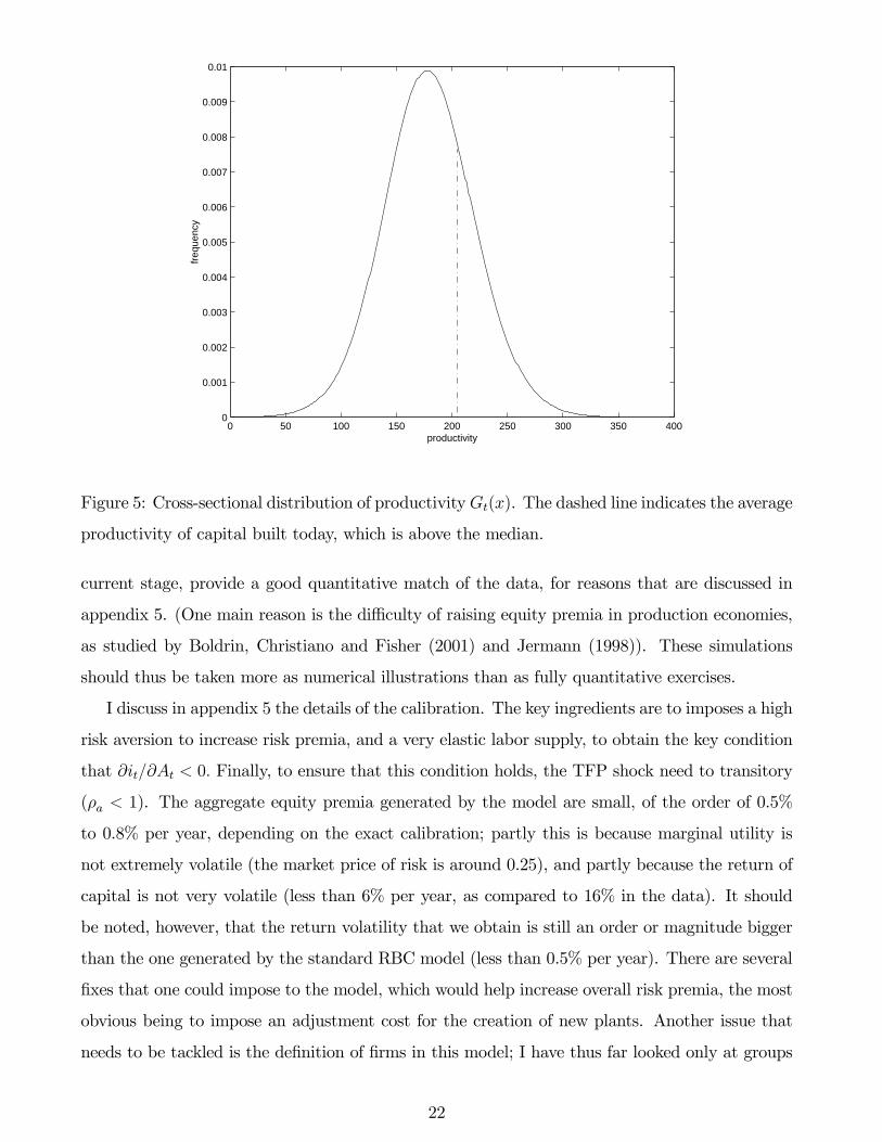
xt = iαt . This is depicted in figure 5 below, where the current optimal productivity is clearly above

the median of the distribution of x. Hence, the twist of the relative price of low-productivity vs.

high-productivity capital does lead to changes in the value of the aggregate capital stock.19

The interpretation is the same as the one given for the pricing of the individual plants, with

the two related angles:

- With non-responsive wages, the present-value of TFP increases by more than the present-

value of wages, which increases the price of low-productivity plants and decreases the price of

high-productivity plants. With many low-productivity plants in the economy, this increases the

aggregate value of capital.

- A change in i reflects a change in the relative price of labor, with a high i reflecting expensive

labor, which hurts capital, thus ∂V/∂i < 0; in turn, if we choose parameters such that εi,A < 0,

we obtain dV/dA = ∂V/∂i.∂i/∂A > 0 : the stock market is procyclical.

B. Numerical Results

This section gives some results from numerical simulations of the model. These numerical

simulations confirm the qualitative results discussed in the previous section. They do not, at the

18In a standard adjustment cost model, Vt = qtKt where qt is Tobin’s q, an increasing function of the invest-

ment/capital ratio. In this case, variation in q leads to price variation.19The result can also be glimpsed in figure 2 above: Tobin’s q increase for low productivity plants, and decreases

for high productivity, but since there are many more low-productivity units than high productivity units, in the

aggregate Tobin’s q rise: the stock market jumps up.

21

0 50 100 150 200 250 300 350 4000

0.001

0.002

0.003

0.004

0.005

0.006

0.007

0.008

0.009

0.01

productivity

freq

uenc

y

Figure 5: Cross-sectional distribution of productivityGt(x). The dashed line indicates the average

productivity of capital built today, which is above the median.

current stage, provide a good quantitative match of the data, for reasons that are discussed in

appendix 5. (One main reason is the difficulty of raising equity premia in production economies,

as studied by Boldrin, Christiano and Fisher (2001) and Jermann (1998)). These simulations

should thus be taken more as numerical illustrations than as fully quantitative exercises.

I discuss in appendix 5 the details of the calibration. The key ingredients are to imposes a high

risk aversion to increase risk premia, and a very elastic labor supply, to obtain the key condition

that ∂it/∂At < 0. Finally, to ensure that this condition holds, the TFP shock need to transitory

(ρa < 1). The aggregate equity premia generated by the model are small, of the order of 0.5%

to 0.8% per year, depending on the exact calibration; partly this is because marginal utility is

not extremely volatile (the market price of risk is around 0.25), and partly because the return of

capital is not very volatile (less than 6% per year, as compared to 16% in the data). It should

be noted, however, that the return volatility that we obtain is still an order or magnitude bigger

than the one generated by the standard RBC model (less than 0.5% per year). There are several

fixes that one could impose to the model, which would help increase overall risk premia, the most

obvious being to impose an adjustment cost for the creation of new plants. Another issue that

needs to be tackled is the definition of firms in this model; I have thus far looked only at groups

22

of plants, without taking into account the future investment done by these plants. These issues

are discussed in more detail in appendix 5, where I also display the impulse responses to a TFP

shock.

I also examine the consequences of a second shock in this model, a labor tax (or labor supply)

shock. A strand of the business cycle literature has documented that more sources of shocks may

be required, notably because the first-order condition governing labor supply doesn’t hold well in

the data.20 In terms of the cross-sectional differences in returns, this shock may be quantitatively

important since an increase in the labor cost will affect differently low and high productivity

firms; as a result it will also affect the aggregate stock market. Impulse responses to this shock,

shown in the appendix, confirm this; moreover, because output doesn’t rise immediately, the

model delivers the stylized fact that the stock market forecasts (or leads) output.21 This fact

is not matched by adjustment cost models (e.g., Jermann 1998), or by the preferred two-sector

model of Boldrin, Christiano and Fisher (2001), though Lamont’s work (2000) suggests that a

model with planning lags might capture it. We return to this fact in more detail in Section 6.

I next replicate Fama and French’s empirical approach on simulated data from my model.

But first, table 1 gives empirical results similar to those of Fama and French: these are summary

statistics of 10 portfolios sorted by book-to-market, for two different samples. These portfolios

are constructed by sorting firms,at the beginning of each year, by the ratio of their book value

to their market value, and then assigning the 10% with the lowest book-to-market ratio into one

portfolio, the next 10% into a second portfolio, and so on up to the top 10%. (Each year, firms are

sorted anew and assigned to a potentially different portfolio.) Portfolio 1 is a “growth” portfolio

(i.e., low book-to-market) and portfolio 10 is a “value” portfolio (high book-to-market). The

lower table is close to the original results of Fama and French (1992), which go strongly against a

CAPM interpretation. The upper table shows that the early part of the sample is actually more

favorable to the CAPM, though in this case too it fails to account for the cross-section. The

20On the need for more shocks, see e.g. Chari, Kehoe and McGrattan (2004), Hall (1997), Ingram et al. (1991),

and the remarks of Ljungqvist and Sargent (2004, chap. 11, p. 334), and on the difficulties with the labor

supply equation, see Hall (1997) and Mulligan (2001). Gilchrist and Williams (2001) also considered a tax shock,

which was quantitatively important in some of their moment-matching exercises. In my dissertation I consider the

possibility of embodied-technology shocks, as in Krusell, Hercowitz and Greenwood (2000), Christiano and Fisher

(2004), but I do not find them very useful to understand asset prices.21I thank Jonas Fisher for emphasizing this. The fact that the stock market forecasts output growth has

been noted at least since Fischer and Merton (1984), though Stock and Watson (2003) consider it unreliable for

out-of-sample forecasting. See section 6 for some empirical documentation.

23

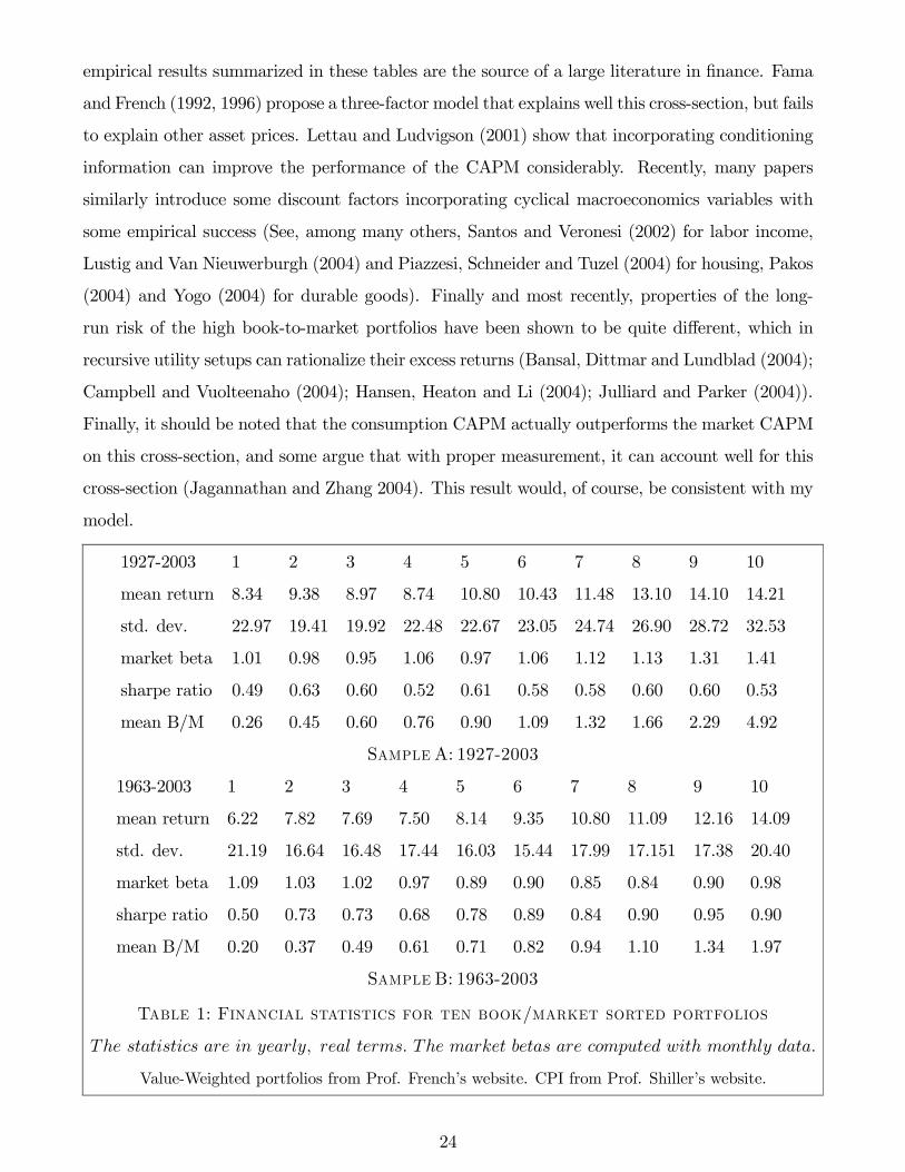
empirical results summarized in these tables are the source of a large literature in finance. Fama

and French (1992, 1996) propose a three-factor model that explains well this cross-section, but fails

to explain other asset prices. Lettau and Ludvigson (2001) show that incorporating conditioning

information can improve the performance of the CAPM considerably. Recently, many papers

similarly introduce some discount factors incorporating cyclical macroeconomics variables with

some empirical success (See, among many others, Santos and Veronesi (2002) for labor income,

Lustig and Van Nieuwerburgh (2004) and Piazzesi, Schneider and Tuzel (2004) for housing, Pakos

(2004) and Yogo (2004) for durable goods). Finally and most recently, properties of the long-

run risk of the high book-to-market portfolios have been shown to be quite different, which in

recursive utility setups can rationalize their excess returns (Bansal, Dittmar and Lundblad (2004);

Campbell and Vuolteenaho (2004); Hansen, Heaton and Li (2004); Julliard and Parker (2004)).

Finally, it should be noted that the consumption CAPM actually outperforms the market CAPM

on this cross-section, and some argue that with proper measurement, it can account well for this

cross-section (Jagannathan and Zhang 2004). This result would, of course, be consistent with my

model.

1927-2003 1 2 3 4 5 6 7 8 9 10

mean return 8.34 9.38 8.97 8.74 10.80 10.43 11.48 13.10 14.10 14.21

std. dev. 22.97 19.41 19.92 22.48 22.67 23.05 24.74 26.90 28.72 32.53

market beta 1.01 0.98 0.95 1.06 0.97 1.06 1.12 1.13 1.31 1.41

sharpe ratio 0.49 0.63 0.60 0.52 0.61 0.58 0.58 0.60 0.60 0.53

mean B/M 0.26 0.45 0.60 0.76 0.90 1.09 1.32 1.66 2.29 4.92

S A: 1927-2003

1963-2003 1 2 3 4 5 6 7 8 9 10

mean return 6.22 7.82 7.69 7.50 8.14 9.35 10.80 11.09 12.16 14.09

std. dev. 21.19 16.64 16.48 17.44 16.03 15.44 17.99 17.151 17.38 20.40

market beta 1.09 1.03 1.02 0.97 0.89 0.90 0.85 0.84 0.90 0.98

sharpe ratio 0.50 0.73 0.73 0.68 0.78 0.89 0.84 0.90 0.95 0.90

mean B/M 0.20 0.37 0.49 0.61 0.71 0.82 0.94 1.10 1.34 1.97

S B: 1963-2003

T 1: F /

The statistics are in yearly, real terms. The market betas are computed with monthly data.

Value-Weighted portfolios from Prof. French’s website. CPI from Prof. Shiller’s website.

24

Table 2 gives the results obtained from a simulated panel data set from my model.22 Qualita-

tively, the sign of the relation is reproduced: high book-to-market portfolios have higher average

returns. The magnitude of the relation is however not matched. This failure is in part attribut-

able to the relatively small aggregate risk premia in the model (another part is due to the fact

that these plants do not reinvest). The pattern that high book-to-market portfolios are more

volatile is stronger in the model than in the data. (However, note that the U-shaped pattern of

volatilities is also evident in the data for the 1963-2003 sample at least.) Of course, in the model,

these return differentials are fully explained by differences in β. More work remains to be done

to obtain a full quantitative match of the data, and to understand why the market βs do not

account for return differentials.

Calibration C 1 2 3 4 5 6 7 8 9 10

ER 0.39 0.44 0.49 0.54 0.59 0.64 0.71 0.82 0.99 1.88

σ(R) 5.23 4.95 4.74 4.55 4.35 4.16 3.97 3.83 4.00 7.78

BM 0.19 0.41 0.47 0.52 0.58 0.64 0.73 0.85 1.09 2.12

T 2: S :

B/M (TFP+L )

The data construction follows Fama and French (1992).

5 Evidence on the Cross-Section of Returns and the Book-to-market effect

I now examine the empirical relevance of the mechanism that I developed in the last section.

The model predicts some correlations between the financial and real characteristics of firms. A key

prediction is that firms which have higher labor productivity x or a higher capital share will have

a lower “operating leverage”. Their operating income will be less sensitive to aggregate shocks.

This property of their cash flows will lead them to have lower βs and lower average returns. In the

model, the low x firms also have more volatile returns than the high x firms;23 and finally the low

x firms have on average a higher book-to-market ratio (since part of productivity shows up in the

market value, but not in the book value). More precisely, equation (4.5) εP (x),A = (1− αst(x)) εi,A

implies that β(x), which is proportional to ∂ER(x)/∂A εP (x),A, is positively related to st(x)

22I follow the portfolio formation rules of Fama and French (1992): firms are sorted each year by book-to-market;

then, with a 2 quarter lag they are assigned to porfolios based on the decile of B/M; and they are reassigned next

year to a new portfolio.23The exception is that the x > xt will be volatile and negatively correlated with the market, see equation (3.6).

25

and thus negatively to x. (Remember that εi,A < 0 for our preferred parameter values, and that

st is a decreasing function of x.) A quantitative prediction is that differences in β and average

returns across stocks should be proportional to differences in inverse capital share st.24

In Section A I examine whether these real characteristics can explain differences of returns

across book-to-market sorted portfolios, and in Section B I look at differences in average returns

across industries.

A. Book-to-market sorted portfolios

In this section, I examine the model’s implications by looking at 10 portfolios of firms, created

by sorting listed firms by book-to-market.25 As noted by Fama and French (1992) and others,

the portfolios with higher book-to-market equity have higher average returns, and the spread in

returns is large: the difference between the highest and lowest return is around 7% annually (See

Section 4B for some statistics and a quick literature review). The interpretation for these return

differences that I propose is that the sort on book-to-market is effectively a sort on productivity

x. High book-to-market are low productivity firms which have a high operating leverage, are

more sensitive to aggregate shocks, and have thus higher average returns. I proceed to check all

these associations, by measuring directly productivity, operating leverage, sensitivity to aggregate

shocks and mean returns for these portfolios.

Of course, in my theory, the differences in sensitivities should show up in differences in market

βs; we know in advance from the finance literature that they won’t. In this section, I will discard

the evidence on β and relate directly real attributes that determine riskiness in my model with

mean average returns.26

24However, the proportionality factor, related to the sensitivity of consumption to shocks and the market price

of risk, requires to impose the specification of the full model (including preferences and the structure of shocks),

which I do not want to do.25Each year, firms are ranked by their book-to-market equity, and assigned by deciles to one of the 10 portfolios.

The lowest B/M portfolio is 1 (also called “growth”) and the highest B/M is 10 (“value”). Source: Compustat

annual data, 1963-2002.26There are two reasons why despite this, the predictions are interesting. First, even if the return differentials

across book-to-market were explained by differences in betas, it would be interesting to understand why some

firms bear a disproportionate share of the cyclical variation (i.e. where the heterogeneity in book-to-market comes

from). Second, we can look directly at the correlation between the characteristic and average return, implied by

the model, and discard the information in β, for instance because it is ill-measured. In a sense, this is just a matter

of “fixing” the utility function that closes the model (but of course, it remains to check if with this modification,

the betas would still be correlated with productivity).

26

High Book-to-Market have a low capital share and a low productivity/profitability

As explained above and proved in the appendix, I can approximate the measure of operating

leverage st(x)by the inverse of the capital share of a firm. In practice, constructing firm-level

value added is a hard task. I thus proxy the capital share by the ratio of operating income to

sales, and the first line of table 3 gives, for each portfolio, the average (over time) of the ratio

sales/operating income.27 This ratio is strongly upward sloping: high book-to-market firms tend

indeed to have a small capital share. This is a first success for our proposed interpretation: high

book-to-market firms have higher operating leverage.

I now examine whether we can trace this back to differences in labor productivity. Previous

work has shown that high book-to-market firms have low profitability (Fama and French (1995)).

In table 3, I reproduce their main finding: the ratio of operating income to book equity is de-

creasing in book-to-market. There are several ways in which one can measure more precisely

labor productivity; one would like to have the value added per employee. As noted above, Dwyer

(2001) found a negative correlation of -0.3 in plant-level data between book-to-market and pro-

ductivity. In my data set, I can proxy labor productivity by the sales/employee ratio or the

operating income per employee. The second ratio is indeed strongly downward sloping, but the

first one is hump-shaped. Overall, I conclude that high book-to-market firms tend to have lower

productivity/profitability per employee. This is not really surprising in the light of the finance

literature which views these firms as “distressed”, i.e. experiencing (temporary or permanent)

difficulties.28

Portfolios i = 1 2 3 4 5 6 7 8 9 10SalesOp. Inc.

5.42 6.26 6.89 7.36 7.59 7.82 7.94 8.68 9.44 12.39Op.Inc.

Employees1.25 1.03 0.98 1.00 1.04 1.08 1.03 0.93 0.83 0.62

SalesEmployees

0.89 0.86 0.90 1.00 1.06 1.15 1.08 1.04 1.02 0.95Op. Inc.Book

0.50 0.42 0.37 0.35 0.32 0.30 0.28 0.26 0.24 0.20

T 3: T M ,

Source: Compustat, 1963-2002. Portfolios sorted by increasing book-to-market each year.

Lines 2&3: the mean refers to the mean of series: Portfolio variable/Aggregate variable

High book-to-market firms have more cyclical operating income27The variables here are portfolio aggregates: for instance, the first line is total sales of the portfolio divided by

the total operating income. This is akin to considering value-weighted portfolios.28It is possible to add transitory idiosyncratic productivity shocks to the model, without changing its

implications.

27

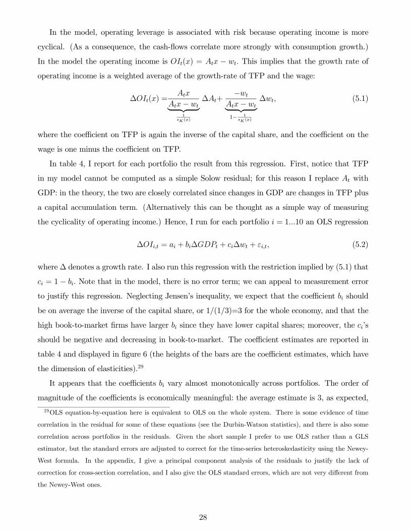
In the model, operating leverage is associated with risk because operating income is more

cyclical. (As a consequence, the cash-flows correlate more strongly with consumption growth.)

In the model the operating income is OIt(x) = Atx − wt. This implies that the growth rate ofoperating income is a weighted average of the growth-rate of TFP and the wage:

∆OIt(x) =Atx

Atx− wt1

sK (x)

∆At+−wt

Atx− wt1− 1

sK (x)

∆wt, (5.1)

where the coefficient on TFP is again the inverse of the capital share, and the coefficient on the

wage is one minus the coefficient on TFP.

In table 4, I report for each portfolio the result from this regression. First, notice that TFP

in my model cannot be computed as a simple Solow residual; for this reason I replace At with

GDP: in the theory, the two are closely correlated since changes in GDP are changes in TFP plus

a capital accumulation term. (Alternatively this can be thought as a simple way of measuring

the cyclicality of operating income.) Hence, I run for each portfolio i = 1...10 an OLS regression

∆OIi,t = ai + bi∆GDPt + ci∆wt + εi,t, (5.2)

where∆ denotes a growth rate. I also run this regression with the restriction implied by (5.1) that

ci = 1− bi. Note that in the model, there is no error term; we can appeal to measurement errorto justify this regression. Neglecting Jensen’s inequality, we expect that the coefficient bi should

be on average the inverse of the capital share, or 1/(1/3)=3 for the whole economy, and that the

high book-to-market firms have larger bi since they have lower capital shares; moreover, the ci’s

should be negative and decreasing in book-to-market. The coefficient estimates are reported in

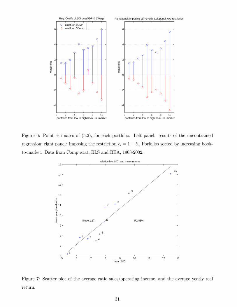
table 4 and displayed in figure 6 (the heights of the bars are the coefficient estimates, which have

the dimension of elasticities).29

It appears that the coefficients bi vary almost monotonically across portfolios. The order of

magnitude of the coefficients is economically meaningful: the average estimate is 3, as expected,

29OLS equation-by-equation here is equivalent to OLS on the whole system. There is some evidence of time

correlation in the residual for some of these equations (see the Durbin-Watson statistics), and there is also some

correlation across portfolios in the residuals. Given the short sample I prefer to use OLS rather than a GLS

estimator, but the standard errors are adjusted to correct for the time-series heteroskedasticity using the Newey-

West formula. In the appendix, I give a principal component analysis of the residuals to justify the lack of

correction for cross-section correlation, and I also give the OLS standard errors, which are not very different from

the Newey-West ones.

28

and there is a fair amount of dispersion.30 Some of these coefficients are not statistically significant

though, because portfolio-level income growth is quite volatile. The ci are negative (except c7) and

tend to decrease when we move from low book-to-market to high book-to-market, as predicted,

but the pattern is not fully monotonic. It is however supportive that the high book-to-market have

a much larger sensitivity to labor compensation than the low book-to-market. To my knowledge,

neither empirical pattern had been noted previously. When we impose the restriction, we see a

clear increasing pattern of coefficients.

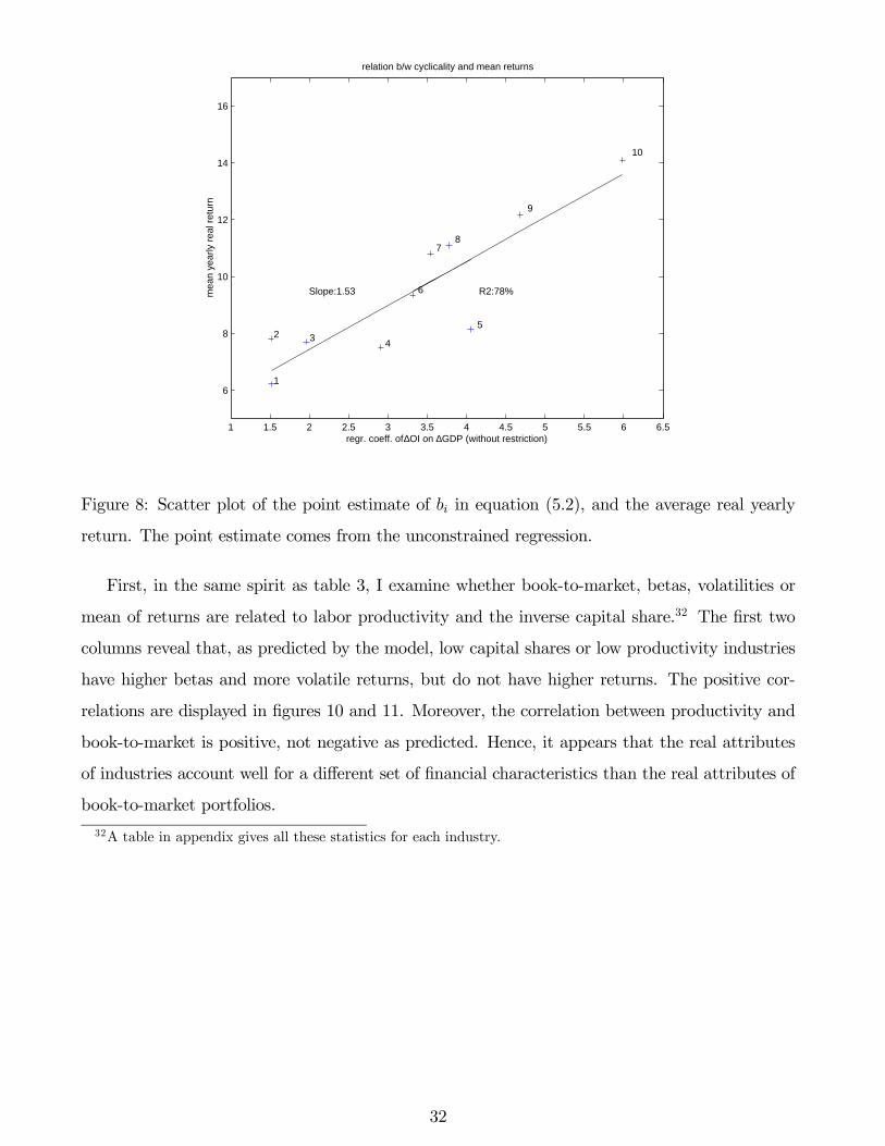
One way to summarize the strength of these correlations is to show that they account for a

large share of the variance of returns. Figure 7 gives the relation between our empirical estimate

of st(x), the mean of the sales/operating income ratio (the mean inverse of the “capital share”)

and average returns, and figure 8 displays similarly the relation between the regression coefficient

on GDP (from table 4a) and average returns. The fit is relatively good, which suggests that these

variables account for the underlying risk of these portfolios. Note that the quantitative prediction

underlined above implies that figure 7 and 8 should be straight lines (not any kind of monotonic

function), since the differences in returns are proportional to differences in inverse capital share;

hence the high R2 are supportive.

30If we were measuring capital shares in table 3, we could check that the estimates for bi are indeed the inverse

of the capital shares of each portfolio. However, we divide by sales, which are greater than value added, hence this

direct test is not possible.

29

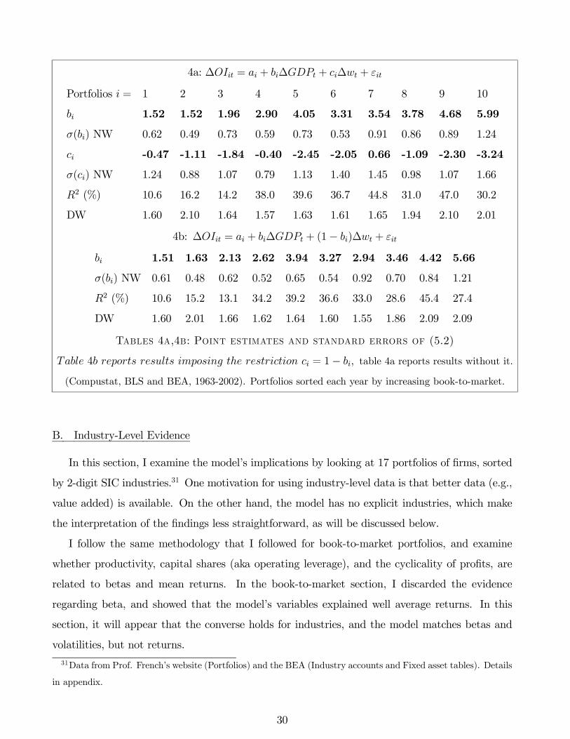
4a: ∆OIit = ai + bi∆GDPt + ci∆wt + εit

Portfolios i = 1 2 3 4 5 6 7 8 9 10

bi 1.52 1.52 1.96 2.90 4.05 3.31 3.54 3.78 4.68 5.99

σ(bi) NW 0.62 0.49 0.73 0.59 0.73 0.53 0.91 0.86 0.89 1.24

ci -0.47 -1.11 -1.84 -0.40 -2.45 -2.05 0.66 -1.09 -2.30 -3.24

σ(ci) NW 1.24 0.88 1.07 0.79 1.13 1.40 1.45 0.98 1.07 1.66

R2 (%) 10.6 16.2 14.2 38.0 39.6 36.7 44.8 31.0 47.0 30.2

DW 1.60 2.10 1.64 1.57 1.63 1.61 1.65 1.94 2.10 2.01

4b: ∆OIit = ai + bi∆GDPt + (1− bi)∆wt + εit

bi 1.51 1.63 2.13 2.62 3.94 3.27 2.94 3.46 4.42 5.66

σ(bi) NW 0.61 0.48 0.62 0.52 0.65 0.54 0.92 0.70 0.84 1.21

R2 (%) 10.6 15.2 13.1 34.2 39.2 36.6 33.0 28.6 45.4 27.4

DW 1.60 2.01 1.66 1.62 1.64 1.60 1.55 1.86 2.09 2.09

T 4 ,4 : P (5.2)

Table 4b reports results imposing the restriction ci = 1− bi, table 4a reports results without it.(Compustat, BLS and BEA, 1963-2002). Portfolios sorted each year by increasing book-to-market.

B. Industry-Level Evidence

In this section, I examine the model’s implications by looking at 17 portfolios of firms, sorted

by 2-digit SIC industries.31 One motivation for using industry-level data is that better data (e.g.,

value added) is available. On the other hand, the model has no explicit industries, which make

the interpretation of the findings less straightforward, as will be discussed below.

I follow the same methodology that I followed for book-to-market portfolios, and examine

whether productivity, capital shares (aka operating leverage), and the cyclicality of profits, are

related to betas and mean returns. In the book-to-market section, I discarded the evidence

regarding beta, and showed that the model’s variables explained well average returns. In this

section, it will appear that the converse holds for industries, and the model matches betas and

volatilities, but not returns.

31Data from Prof. French’s website (Portfolios) and the BEA (Industry accounts and Fixed asset tables). Details

in appendix.

30

0 2 4 6 8 10

−4

−2

0

2

4

6

portfolios from low to high book−to−market

ela

stic

ities

Reg. Coeffs of ∆OI on ∆GDP & ∆Wage

coeff. on ∆GDPcoeff. on ∆Comp.

0 2 4 6 8 10

−4

−2

0

2

4

6

portfolios from low to high book−to−market e

last

iciti

es

Right panel: imposing c(i)=1−b(i); Left panel: w/o restriction;

Figure 6: Point estimates of (5.2), for each portfolio. Left panel: results of the uncontrained

regression; right panel: imposing the restriction ci = 1− bi. Porfolios sorted by increasing book-to-market. Data from Compustat, BLS and BEA, 1963-2002.

5 6 7 8 9 10 11 12 136

7

8

9

10

11

12

13

14

15

1

2 34

5

6

78

9

10

R2:88%Slope:1.17

mean S/OI

mea

n ye

arly

rea

l ret

urn

relation b/w S/OI and mean returns

Figure 7: Scatter plot of the average ratio sales/operating income, and the average yearly real

return.

31

1 1.5 2 2.5 3 3.5 4 4.5 5 5.5 6 6.5

6

8

10

12

14

16

1

2 3 4

5

6

78

9

10

R2:78%Slope:1.53

regr. coeff. of ∆OI on ∆GDP (without restriction)

mea

n ye

arly

rea

l ret

urn

relation b/w cyclicality and mean returns

Figure 8: Scatter plot of the point estimate of bi in equation (5.2), and the average real yearly

return. The point estimate comes from the unconstrained regression.

First, in the same spirit as table 3, I examine whether book-to-market, betas, volatilities or

mean of returns are related to labor productivity and the inverse capital share.32 The first two

columns reveal that, as predicted by the model, low capital shares or low productivity industries

have higher betas and more volatile returns, but do not have higher returns. The positive cor-

relations are displayed in figures 10 and 11. Moreover, the correlation between productivity and

book-to-market is positive, not negative as predicted. Hence, it appears that the real attributes

of industries account well for a different set of financial characteristics than the real attributes of

book-to-market portfolios.

32A table in appendix gives all these statistics for each industry.

32

1/Capital Share

mean real return -0.14

std real return 0.80

market β 0.79

book/market (beg. of period) 0.02

VA/Empl (rel.)

-0.02

-0.57

-0.65

0.47

β∆OI,∆GDP

0.02

0.58

0.41

0.40

βrestricted∆OI,∆GDP

0.00

0.58

0.43

0.25

T 5: Correlations between productivity, financial and economic variables across industries

Sources: see appendix 8.

As I did for book-to-market, I estimate the equation (5.2) for the cyclical sensitivity of profits,

again with and without imposing the restriction; the point estimates are displayed in figure 9

(the full table of results is available in appendix 8). I examine whether these point estimates

relate to either book-to-market, betas, volatilities or mean returns, in the last two columns of

table 5. As the theory predicts, more cyclical operating income is positively correlated with

betas and volatilities, but again the correlation with mean returns is nil, and the correlation with

book-to-market has the wrong sign.

These results can be attributed to the failure of the CAPM for the industry portfolios, as

documented by Fama and French (1997): the market betas explain only a small share of the

variance of stock returns, hence though my model explains the betas well, it fails to explain the

returns.

Difficulties with Cross-Industry Correlations

There are at least two particularities of industries which the model does not capture. First,

real-life industries have different elasticities of demand and some are more cyclical, for the simple

reason that they produce goods which demand vary more (e.g., luxuries or durables). Second,

there are different production technologies, which in the model can be captured simply as different

α. This second fact does not really preclude the model from making predictions: changes in the

aggregate variable i will still drive all industries returns, but now their reactions will also differ

because they have different α. Further work will examine these issues in more detail. In ongoing

work, I use the NBER manufacturing productivity database and the Compustat data set to

continue the above analysis at a finer level. I also plan to look at the two dimensions of the data

set, i.e. examining how the risk of an industry evolve over time, in relation to the evolution of

the real variables. This is motivated by Fama and French (1997), who show that the estimates

of risk at the industry level vary over time.

33

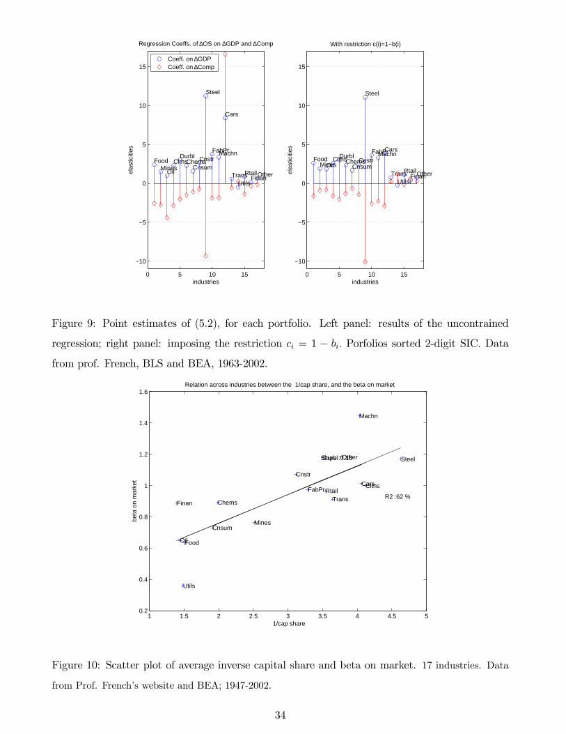
0 5 10 15

−10

−5

0

5

10

15

FoodMines

Oil

ClthsDurbl

ChemsCnsum

Cnstr

Steel

FabPrMachn

Cars

TransUtils

RtailFinanOther

Regression Coeffs. of ∆OS on ∆GDP and ∆Comp

industries

elas

ticiti

es

Coeff. on ∆GDPCoeff. on ∆Comp

0 5 10 15

−10

−5

0

5

10

15

FoodMinesOil

ClthsDurblChems

CnsumCnstr

Steel

FabPrMachnCars

TransUtils

RtailFinanOther

With restriction c(i)=1−b(i)

industriesel

astic

ities

Figure 9: Point estimates of (5.2), for each portfolio. Left panel: results of the uncontrained

regression; right panel: imposing the restriction ci = 1 − bi. Porfolios sorted 2-digit SIC. Datafrom prof. French, BLS and BEA, 1963-2002.

1 1.5 2 2.5 3 3.5 4 4.5 50.2

0.4

0.6

0.8

1

1.2

1.4

1.6

Food

Mines

Oil

Clths

Durbl

Chems

Cnsum

Cnstr

Steel

FabPr

Machn

Cars

Trans

Utils

Rtail

Finan

Other

Relation across industries between the 1/cap share, and the beta on market

1/cap share

beta

on

mar

ket

R2 :62 %

Slope :0.18

Figure 10: Scatter plot of average inverse capital share and beta on market. 17 industries. Data

from Prof. French’s website and BEA; 1947-2002.

34

0 50 100 150 200 2500.2

0.4

0.6

0.8

1

1.2

1.4

1.6

Food

Mines

Oil

Clths

Durbl

Chems

Cnsum

Cnstr

Steel

FabPr

Machn

Cars

Trans

Utils

Rtail

Finan

Other

Relation across industries between the Productivity, and the beta on market

Productivity

beta

on

mar

ket

R2 :42 %

Slope :−0.01

Figure 11: Scatter plot of average labor productivity (relative to the average) and beta on market.

17 industries. Data from Prof. French’s website and BEA; 1947-2002.

6 Evidence using Aggregate Data: Stock Market Cyclicality

To consider the model’s aggregate implications, I follow Cochrane (1991) and Hall (2001) who

derive implications without specifying a full general equilibrium model. Instead I use only the

production side of the model, backing out the value of the stock market from some model rela-

tionships and macroeconomic time series. Using this approach, the model captures quantitatively

the cyclical movements of stock market value. In the data, the ratio of gross investment to net

jobs created is countercyclical. In the model, this means that the capital intensity of new plants

it is high in recessions, and the key condition ∂it/∂At < 0 that gives a procyclical stock market

is thus verified in the data: variations in the relative scarcity of capital and labor generate large

movements in capital value. In what follows, I contrast the results obtained from my putty-clay

formulation with those implied by a standard adjustment cost model and find that it does better

at capturing the cyclicality of the stock returns: the stock market return forecasts the business

cycle.

Concretely, I use the result 3:

Vt =itα

Ytiαt− (1− α)Nt ,

35

to construct Vt, the ex-dividend value of aggregate capital, given data from macroeconomic time

series, and compare it to the aggregate stock market value. (it is the capital intensity of new

plants; Nt is total hours worked; Yt is the productive capacity, or GDP divided by TFP.) To use

this formula and find Vt, I need to compute on it, Nt, and Yt. The following paragraph explains

how I extract my model’s series from the data.

I take Nt directly as an index of total hours worked, and I use the model law of motion Nt+1 =

(1−δ)Nt+ht to compute ht given an assumed value for δ. Then, I use the model identity it = It/htan NIPA data on aggregate investment It to construct it, the capital intensity of new jobs. Finally,

to obtain Yt, I iterate on the second law of motion Yt+1 = (1−δ)Yt+iαt ht. I need for this to assumea value for α and Y0. Finally, I use data on GDP Yt to display Vt/Yt, the stock-market / GDP ratio,

implied by the model. I also compute the return on aggregate capital Rt,t+1 = (Vt+1 +Dt+1)/Vt,

where the “dividend” is, from the model, Dt+1 = Yt+1 −wt+1Nt+1 = Yt+1 (1− sL,t+1) . The seriesfor the labor share sL,t+1 is taken directly from the data. This dividend component turns out to

be quantitatively unimportant relative to the capital gain part.

There are few degrees of freedom implicit in this analysis: δ,α and Y0. The following results

set α = 0.3 and δ = 0.12, and use annual data. (The data sources are listed in the appendix 9,

with a discussion of the sensitivity of these results.) Figure 12 gives the path for ht, inferred as

described above: ht, the quasi-difference in hours, trends upward because of employment growth,

but it is volatile, falling a lot in recessions. Figure 13 shows it, the investment per new job (or

capital intensity of new jobs); this variable also has a long-run trend, reflecting capital deepening,

but the spikes, due to the troughs of ht, are substantial. These spikes in it create downturns

in the stock-market, as explained in Section 3; the stock market value is displayed in figure 14.

This graph deserves some comments. First, note that there is little point in fitting the average

value of the stock market, because the model gives the value of the total stock of capital - but

we know that a big part of the stock of capital is not publicly traded, and another part of it is

actually owned by bondholders (not included here).33 Second, some recent work (e.g., Hall (2001),

Greenwood and Jovanovic (1999), Hobijn and Jovanovic (2001), Laitner and Stolyarov (2003))

examines the low-frequency movements in the stock-market: why was the market so low in the

late 70s to mid 80s, with Tobin’s q well below 1, and why was it so high in the 90s? The model

is not designed to look at this question, since its medium-run implications are the same as the

standard neoclassical model, with the stock market reflecting the quantity of capital. What the

33However, I did not rescale the series of Vt, since its level turns out to be consistent with the data series.

36

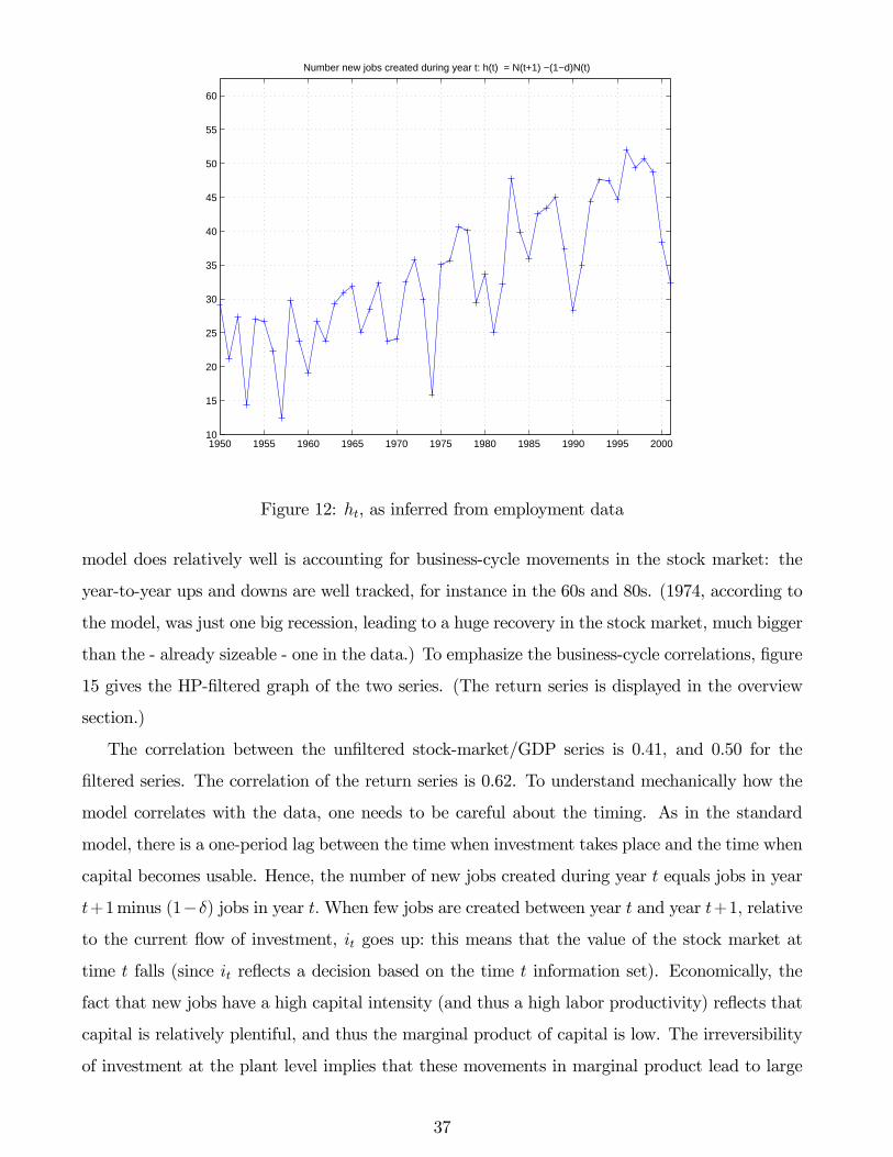
1950 1955 1960 1965 1970 1975 1980 1985 1990 1995 200010

15

20

25

30

35

40

45

50

55

60

Number new jobs created during year t: h(t) = N(t+1) −(1−d)N(t)

Figure 12: ht, as inferred from employment data

model does relatively well is accounting for business-cycle movements in the stock market: the

year-to-year ups and downs are well tracked, for instance in the 60s and 80s. (1974, according to

the model, was just one big recession, leading to a huge recovery in the stock market, much bigger

than the - already sizeable - one in the data.) To emphasize the business-cycle correlations, figure

15 gives the HP-filtered graph of the two series. (The return series is displayed in the overview

section.)

The correlation between the unfiltered stock-market/GDP series is 0.41, and 0.50 for the

filtered series. The correlation of the return series is 0.62. To understand mechanically how the

model correlates with the data, one needs to be careful about the timing. As in the standard

model, there is a one-period lag between the time when investment takes place and the time when

capital becomes usable. Hence, the number of new jobs created during year t equals jobs in year

t+1minus (1−δ) jobs in year t.When few jobs are created between year t and year t+1, relative

to the current flow of investment, it goes up: this means that the value of the stock market at

time t falls (since it reflects a decision based on the time t information set). Economically, the

fact that new jobs have a high capital intensity (and thus a high labor productivity) reflects that

capital is relatively plentiful, and thus the marginal product of capital is low. The irreversibility

of investment at the plant level implies that these movements in marginal product lead to large

37

1950 1955 1960 1965 1970 1975 1980 1985 1990 1995 2000

10

15

20

25

30

35

40

45

50

55

i = capital intensity of new investment

Figure 13: it = It/ht, the capital intensity of new investment

1950 1955 1960 1965 1970 1975 1980 1985 1990 1995 200020

30

40

50

60

70

80

90

100

110

120

130Stock Mkt / GDP (%)

Model:PCData

Figure 14: U.S. Stock Market Value divided by GDP, Data and Putty-Clay (PC) Model

38

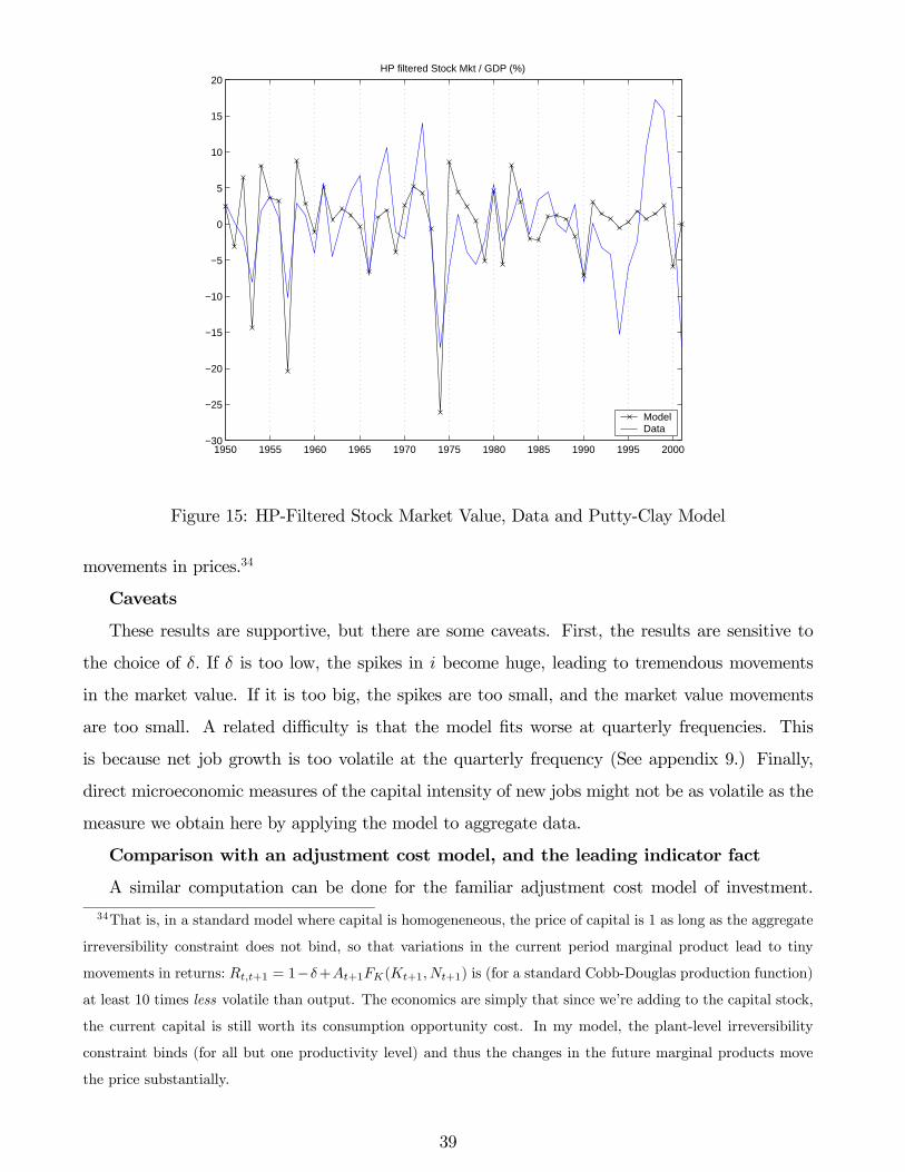
1950 1955 1960 1965 1970 1975 1980 1985 1990 1995 2000−30

−25

−20

−15

−10

−5

0

5

10

15

20HP filtered Stock Mkt / GDP (%)

ModelData

Figure 15: HP-Filtered Stock Market Value, Data and Putty-Clay Model

movements in prices.34

Caveats

These results are supportive, but there are some caveats. First, the results are sensitive to

the choice of δ. If δ is too low, the spikes in i become huge, leading to tremendous movements

in the market value. If it is too big, the spikes are too small, and the market value movements

are too small. A related difficulty is that the model fits worse at quarterly frequencies. This

is because net job growth is too volatile at the quarterly frequency (See appendix 9.) Finally,

direct microeconomic measures of the capital intensity of new jobs might not be as volatile as the

measure we obtain here by applying the model to aggregate data.

Comparison with an adjustment cost model, and the leading indicator fact

A similar computation can be done for the familiar adjustment cost model of investment.

34That is, in a standard model where capital is homogeneneous, the price of capital is 1 as long as the aggregate

irreversibility constraint does not bind, so that variations in the current period marginal product lead to tiny

movements in returns: Rt,t+1 = 1−δ+At+1FK(Kt+1, Nt+1) is (for a standard Cobb-Douglas production function)

at least 10 times less volatile than output. The economics are simply that since we’re adding to the capital stock,

the current capital is still worth its consumption opportunity cost. In my model, the plant-level irreversibility

constraint binds (for all but one productivity level) and thus the changes in the future marginal products move

the price substantially.

39

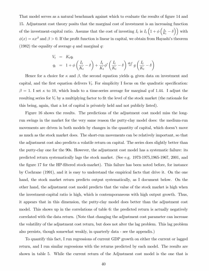
That model serves as a natural benchmark against which to evaluate the results of figure 14 and

15. Adjustment cost theory posits that the marginal cost of investment is an increasing function

of the investment-capital ratio. Assume that the cost of investing It is It 1 + φ ItKt− δ with

φ(x) = κxβ and β > 0. If the profit function is linear in capital, we obtain from Hayashi’s theorem

(1982) the equality of average q and marginal q:

Vt = Ktqt

qt = 1 + φItKt− δ +

ItKt

φItKt− δ

def= g

ItKt− δ

Hence for a choice for κ and β, the second equation yields qt given data on investment and

capital, and the first equation delivers Vt. For simplicity I focus on the quadratic specification:

β = 1. I set κ to 10, which leads to a time-series average for marginal q of 1.44. I adjust the

resulting series for Vt by a multiplying factor to fit the level of the stock market (the rationale for

this being, again, that a lot of capital is privately held and not publicly listed).

Figure 16 shows the results. The predictions of the adjustment cost model miss the long-

run swings in the market for the very same reason the putty-clay model does: the medium-run

movements are driven in both models by changes in the quantity of capital, which doesn’t move

as much as the stock market does. The short-run movements can be relatively important, so that

the adjustment cost also predicts a volatile return on capital. The series does slightly better than

the putty-clay one for the 90s. However, the adjustment cost model has a systematic failure: its

predicted return systematically lags the stock market. (See e.g. 1973-1975,1965-1967, 2001, and

the figure 17 for the HP-filtered stock-market). This failure has been noted before, for instance

by Cochrane (1991), and it is easy to understand the empirical facts that drive it. On the one

hand, the stock market return predicts output systematically, as I document below. On the

other hand, the adjustment cost model predicts that the value of the stock market is high when

the investment-capital ratio is high, which is contemporaneous with high output growth. Thus,

it appears that in this dimension, the putty-clay model does better than the adjustment cost

model. This shows up in the correlations of table 6: the predicted return is actually negatively

correlated with the data return. (Note that changing the adjustment cost parameter can increase

the volatility of the adjustment cost return, but does not alter the lag problem. This lag problem

also persists, though somewhat weakly, in quarterly data - see the appendix.)

To quantify this fact, I run regressions of current GDP growth on either the current or lagged

return, and I run similar regressions with the returns predicted by each model. The results are

shown in table 5. While the current return of the Adjustment cost model is the one that is

40

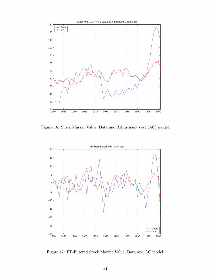
1950 1955 1960 1965 1970 1975 1980 1985 1990 1995 200020

30

40

50

60

70

80

90

100

110

120

130Stock Mkt / GDP (%) : Data and Adjustment Cost Model

DataAC

Figure 16: Stock Market Value, Data and Adjustment cost (AC) model.

1950 1955 1960 1965 1970 1975 1980 1985 1990 1995 2000−30

−25

−20

−15

−10

−5

0

5

10

15

20HP filtered Stock Mkt / GDP (%)

ModelData

Figure 17: HP-Filtered Stock Market Value, Data and AC model.

41

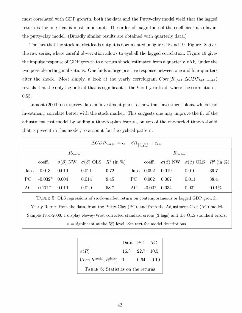
most correlated with GDP growth, both the data and the Putty-clay model yield that the lagged

return is the one that is most important. The order of magnitude of the coefficient also favors

the putty-clay model. (Broadly similar results are obtained with quarterly data.)

The fact that the stock market leads output is documented in figures 18 and 19. Figure 18 gives

the raw series, where careful observation allows to eyeball the lagged correlation. Figure 19 gives

the impulse response of GDP growth to a return shock, estimated from a quarterly VAR, under the

two possible orthogonalizations. One finds a large positive response between one and four quarters

after the shock. Most simply, a look at the yearly correlogram Corr(Rt,t+1,∆GDPt+k,t+k+1)

reveals that the only lag or lead that is significant is the k = 1 year lead, where the correlation is

0.55.

Lamont (2000) uses survey data on investment plans to show that investment plans, which lead

investment, correlate better with the stock market. This suggests one may improve the fit of the

adjustment cost model by adding a time-to-plan feature, on top of the one-period time-to-build

that is present in this model, to account for the cyclical pattern.

∆GDPt→t+1 = α+ βR{t→t+1t−1→t

+ εt+1

Rt→t+1

coeff. σ(β) NW σ(β) OLS R2 (in %)

data -0.013 0.019 0.021 0.72

PC -0.032* 0.004 0.014 9.45

AC 0.171* 0.019 0.020 58.7

Rt−1→t

coeff. σ(β) NW σ(β) OLS R2 (in %)

data 0.092 0.019 0.016 39.7

PC 0.062 0.007 0.011 38.4

AC -0.002 0.034 0.032 0.01%

T 5: OLS regressions of stock—market return on contemporaneous or lagged GDP growth.

Yearly Return from the data, from the Putty-Clay (PC), and from the Adjustment Cost (AC) model.

Sample 1951-2000. I display Newey-West corrected standard errors (3 lags) and the OLS standard errors.

∗ = significant at the 5% level. See text for model descriptions.

Data PC AC

σ(R) 16.3 22.7 10.5

Corr(Rmodel, Rdata) 1 0.64 -0.19

T 6: Statistics on the returns

42

1955 1960 1965 1970 1975 1980 1985 1990 1995 2000−30

−20

−10

0

10

20

30

40Stock Market return and GDP growth (multiplied by 5)

return5∆logGDP

Figure 18: GDP growth (crosses) and US Stock Market Return. 1955-2002, yearly data from BEA

and CRSP. Real GDP growth is multiplied by 5 for comparable scale. Note the leading indicator fact,

e.g. 2000, 1981;1975;1969;1957.

0 5 10 15 20

−0.4

−0.2

0

0.2

0.4

0.6

0.8

1

1.2

1.4 IR of ∆logGDP to a one std deviation return shock

quarters after shock

∆lo

gGD

P

0 5 10 15 20

−0.4

−0.2

0

0.2

0.4

0.6

0.8

1

1.2

1.4 orthogonalization B

quarters after shock

∆lo

gGD

P

Figure 19: Impulse response of GDP growth to a return shock. Derived from quarterly VAR with 8

lags (1947-2003). Left panel: orthogonalization with return=0 at t=0 if GDP shock; right panel: gdp=0

at t=0 if return shock.

43

7 Conclusions

This paper showed that introducing a putty-clay technology in a stochastic growth model

leads to interesting new asset pricing implications which help us understand both the time series

movements in the aggregate stock market, and the differences of expected returns across assets.

This work complements Gilchrist and Williams (2000) who found that the putty-clay technology

also delivers interesting business cycle implications. Many of these business cycle implications

are maintained in the simple variant I develop, which may prove useful for other applications.

The use of this putty-clay technology allowed me to link real sources of risk with financial

measures of risk. This approach stands in contrast to the standard practice in finance of estimating

the assets’ betas as free parameters. Little research in empirical finance and macroeconomics

addresses the question, why are some firms more risky and more cyclical? This topic is important

for macroeconomics, since firm heterogeneity in response to aggregate shocks implies that some

firms account for a large fraction of macroeconomic volatility and play an important role in

aggregate fluctuations. However, a limitation of my approach is that it does not explain why

return differentials cannot be traced to differences in consumption or market betas, which is the

subject of an already very large literature in empirical finance.

The substantive issues that this paper tackles are still not fully resolved, suggesting fruitful

directions for future research. A few facts may help us distinguish among the competing expla-

nations of the correlation between book-to-market ratio and returns. First, at the firm level,

productivity, inverse capital shares and cyclicality are related to book-to-market ratios and to

average returns. Second, at the industry level, productivity, inverse capital shares and cyclicality

are related to the market beta and volatility of stocks. Moreover, The book-to-market effect is

completely a within-industry effect: between industries, expected returns do not correlate with

book-to-market. Explicitly modeling industries, taking into account differences in technology or

in the cyclicality of demand, might help. One may also want to incorporate firms size dynamics

in more detail. Finally, recent research in empirical finance suggests that theories that emphasize

time-varying risk fare much better in explaining the return differentials across portfolios. In turn,

the new betas thus obtained will need to be linked to real characteristics.

The aggregate results, while supportive, may seem to require too much rigidity in terms of

capital-labor substitutability. But the alternative adjustment cost model has also unattractive

features and implications. I believe my results give promise for related models that will link labor

movements to firm valuation; labor is a more important input than capital in most industries,

44

and one reason why firms earn quasi-rents is that assembling a team of workers takes time and is

costly. Microfoundations such as these for the valuation of capital deserve more study.

References

1. Antras, Pol. 2003. “Is the U.S. Aggregate Production Function Cobb-Douglas? NewEstimatesof the Elasticity of Substitution”. Working paper.

2. Alvarez, Fernando, and Urban Jermann. 2004. “Using Asset Prices to Measure the Persistenceof the Marginal Utility of Wealth”. Forthcoming, Econometrica.

3. Atkeson, Andrew and Patrick Kehoe. 1999. “Models of Energy Use: Putty-Putty versusPutty-Clay”, American Economic Review, 89:4, 1028-1043.

4. Baily, Martin, Eric Bartelsman and John Haltiwanger. 2001. “Labor Productivity: StructuralChange and Cyclical Dynamics”. Review of Economics and Statistics, August.

5. Bansal, Ravi, Bob Dittmar and Chris Lundblad. 2004. “Consumption, Dividends, and theCross-Section of Equity Returns”. Journal of Finance, forthcoming.

6. Bansal, Ravi, and Amir Yaron. 2004. “Risks for the Long Run”. Journal of Finance, forth-coming.

7. Bartelsman, Eric, and Dunne. 2001. “Understanding Productivity: Lessons from LongitudinalMicrodata” Journal of Economic Literature.

8. Boldrin, Michele, Lawrence Christiano and Jonas Fisher. 2001. “Habit Persistence, AssetReturns and Business Cycle”. American Economic Review 91:1, 149-166.

9. Bresnahan, Timothy, and Daniel Raff. 1991. “Intra-Industry Heterogeneity and the GreatDepression: The American Motor Vehicles Industry, 1929-1935”. The Journal of EconomicHistory, 51:2, 317-331.

10. Caballero, Ricardo, and Mohamed Hammour. 1994. “The Cleansing Effect of Recessions”.American Economic Review, 84:5, 1350-1368.

11. Campbell, John and Tuomo Vuolteenaho. 2004. “Bad Beta, Good Beta”. American EconomicReview, forthcoming.

12. Carlson, Murray, Adlai Fisher and Ron Giammarino. 2004. “Corporate Investment and AssetPrice Dynamics: Implications for the Cross-Section of Returns ”. Forthcoming, Journal ofFinance.

13. Christiano, Lawrence and Jonas Fisher. 2003. “Stock Market and Investment Goods Prices:Implications for Macroeconomics ”. NBER Working Paper #10031.

14. Cochrane, John. 1991. “Production-Based Asset Pricing and the Link Between Stock Returnsand Economic Fluctuations”, Journal of Finance, 46:1, 209:237.

15. Cogley Timothy, and James Nason. 1995. “Output Dynamics in Real-Business-Cycle Models”.American Economic Review, 85:3 492-511.

16. Cooper, Ian. 2003. “Asset Pricing Implications of Non-Convex Adjustment Costs of Invest-ment”. Norwegian School of Management Working Paper.

45

17. Dwyer, Douglas. 2001. “Plant-level productivity and the Market Value of a Firm”. CensusBureau CES working paper.

18. Fisher, Jonas. 2003. “Technology Shocks Matter”. Federal Reserve Bank of Chicago workingpaper.

19. Fama, Eugene and Kenneth French. 1992. “The Cross-Section of Expected Stocks Returns”.Journal of Finance, 47:2, 427-465.

20. Fama, Eugene and Kenneth French. 1995. “Size and Book-to-Market Factors in Earnings andReturns”. Journal of Finance, 50:1., 131-155.

21. Fama, Eugene and Kenneth French. 1996. “Multifactor Explanations of Asset Pricing Anom-alies”. Journal of Finance, 51:1, 55-84.

22. Fama, Eugene and Kenneth French. 1997. “Industry costs of equity”. Journal of FinancialEconomics, 43:2, 153-193.

23. Fama, Eugene and Kenneth French. 1998. “Value versus Growth: The International Evi-dence”. Journal of Finance, 53:6, 1975-1999.

24. Fischer, Stanley and Robert Merton. 1984. “Macroeconomics and Finance: The Role of theStock Market”, Carnegie-Rochester Conference Series on Public Policy,21, pp.57-108.

25. Gala, Vito. 2004. “Investment and Stock Returns”. University of Chicago GSB working paper.

26. Gilchrist, Simon, and John Williams. 2000. “Putty-Clay and Investment: A Business CycleAnalysis”, Journal of Political Economy, 108:5, 928-960.

27. Gomes Joao, Leonid Kogan, and Lu Zhang. 2003. “Equilibrium Cross Section of Returns”.Journal of Political Economy, 114:4, 693-732.

28. Gomme, Paul and Jeremy Greenwood. “On the cyclical allocation of risk”. JEDC, 19:1-2,91-124.

29. Greenwood, Jeremy, Zvi Hercowitz and Per Krusell. 1997. “Long-Run Implications ofInvestment-Specific Technological Change”. American Economic Review, 87:3, 342-362.

30. Greenwood, Jeremy, Zvi Hercowitz and Per Krusell. 2001. “The role of investment-specifictechnological change in the business cycle”. European Economic Review, 40:1, 91-115.

31. Hayashi, Fumio. 1982. “Tobin’s Marginal q and Average q: A Neoclassical Interpretation”.Econometrica, 50:1, 213-224.

32. Hall, Robert. 2001. “The Stock Market and Capital Accumulation”. American EconomicReview, 91:6, 1185-1202.

33. Hansen, Gary and Edward Prescott. 2000. “Capacity Constraints, Asymmetries, and theBusiness Cycle”. Working paper.

34. Hansen, Lars, John Heaton and Nan Li. 2004. “Consumption Strikes Back”. Working paper.

35. Jermann, Urban.1998: “Asset Pricing in Production Economies”, Journal of Monetary Eco-nomics, 41:2, 257-275.

46

36. Johansen, Leif. 1959. “Substitution versus Fixed Production Coefficients in the Theory ofEconomic Growth: A Synthesis”. Econometrica, 27:2, 157-176.

37. Jovanovic, Boyan and Peter Rousseau. 2002. “Moore’s law and Learning-by-doing”. Reviewof Economic Dynamics 5, 346-375.

38. Julliard, Christian and Jonathan Parker. 2004. “Consumption Risk and the Cross-Section ofExpected Returns”. Journal of Political Economy, forthcoming.

39. Lamont, Owen. 2000. “Investment Plans and Stock Returns”, Journal of Finance, 55:6, 2719-2745.

40. Lustig, Hanno, and Stijn Van Nieuwerburgh, 2004. “Housing Collateral, Consumption Insur-ance and Risk Premia: an Empirical Perspective”. Journal of Finance, forthcoming.

41. Lettau Martin and Sydney Ludvigson. 2001. “Resurrecting the (C)CAPM: A Cross-SectionalTest When Risk Premia Are Time-Varying”. Journal of Political Economy. 109:6, 1238:1287.

42. Lettau Martin and Sydney Ludvigson. 2003. “Modelling and measuring the risk-return trade-off”. Working paper.

43. Pakos, Michal. 2004. “Asset Pricing with Durable Goods and Non-Homothetic Preferences”.Working paper, University of Chicago GSB.

44. Perfect, Steven and Kenneth Wiles. 1994. “Alternative constructions of Tobin’s q: An em-pirical comparison”. Journal of Empirical Finance, 1,313:341.

45. Piazzesi, Monika, Martin Schneider and Selale Tuzel. 2004. “Housing, consumption, and assetpricing”. Working paper.

46. Rouwenhorst, G. 1995. “Asset Pricing Implications of Equilibrium Business Cycle Models,”in T. Cooley, ed., Frontiers of Business Cycle Research, Princeton University Press.

47. Santos, Tanos and Pietro Veronesi. “Labor Income and Predictable Stock Returns”. Workingpaper, 2004.

48. Schumpeter, Joseph. 1942. “Capitalism, Socialism and Democracy”. New York: Harper, 1942.

49. Stock, James and Mark Watson. 2003. “Forecasting Output and Inflation: The Role of AssetPrices”. Journal of Economic Literature, 41, 788-829.

50. Syverson, Chad. 2004. “Product Substitutability and Productivity Dispersion”. Review ofEconomics and Statistics, May.

51. Tallarini, Thomas. 2000. “Risk-sensitive real business cycles”. Journal of Monetary Eco-nomics, 45:3, 507-532.

52. Wei, Chao. 2003. “Energy, the stock market, and the putty-clay investment model”. AmericanEconomic Review. 93:1, 311-323.

53. Yogo, Motohiro. 2004. “A Consumption-Based Explanation of Expected Stock Returns”.Working Paper.

54. Zhang, Lu. 2004. “The Value Premium”. Journal of Finance, forthcoming.

47