OPEN FORIS CALC - ethiopiared.org · 3 NFI – Ethiopia, 10 / 2015 PREFACE Open Foris (OF) Calc is...
27
1 OPEN FORIS CALC System for data processing in National Forest Inventory in Ethiopia, Description of settings and scripts of Open Foris Calc Lauri Vesa 4 th October, 2015 Contents Abbreviations and acronyms ............................................................................................................................................................... 2 Preface ............................................................................................................................................................................................... 3 1. Principles of data processing ................................................................................................................................................ 4 1.1. Reporting levels .................................................................................................................................................................... 4 1.2. Data processing chain for trees and stumps ......................................................................................................................... 5 1.3. Allometric equations ............................................................................................................................................................. 8 1.4. Data processing chain for fallen deadwood ........................................................................................................................... 9 2. Sampling design in Calc ..................................................................................................................................................... 10 3.1. Settings .............................................................................................................................................................................. 10 3.2. Base unit area .................................................................................................................................................................... 11 4. Calculation.......................................................................................................................................................................... 13 4.1. List of modules ................................................................................................................................................................... 13 4.2. Categorical variables .......................................................................................................................................................... 13 4.3. R scripts ............................................................................................................................................................................. 15 4.3.1. Tree and stumps ....................................................................................................................................................... 15 4.3.2. CSP data – saplings.................................................................................................................................................. 21 4.3.3. Dead wood ................................................................................................................................................................ 24 4.3.4. Plot ........................................................................................................................................................................... 26 4.4. Error script .......................................................................................................................................................................... 26 References .................................................................................................................................................................................... 27
Transcript of OPEN FORIS CALC - ethiopiared.org · 3 NFI – Ethiopia, 10 / 2015 PREFACE Open Foris (OF) Calc is...

1
OPEN FORIS CALC System for data processing in National Forest Inventory in Ethiopia,
Description of settings and scripts of Open Foris Calc
Lauri Vesa
4th
October, 2015
Contents Abbreviations and acronyms ............................................................................................................................................................... 2
Preface ............................................................................................................................................................................................... 3
1. Principles of data processing ................................................................................................................................................ 4
1.1. Reporting levels .................................................................................................................................................................... 4
1.2. Data processing chain for trees and stumps ......................................................................................................................... 5
1.3. Allometric equations ............................................................................................................................................................. 8
1.4. Data processing chain for fallen deadwood ........................................................................................................................... 9
2. Sampling design in Calc ..................................................................................................................................................... 10
3.1. Settings .............................................................................................................................................................................. 10
3.2. Base unit area .................................................................................................................................................................... 11
4. Calculation .......................................................................................................................................................................... 13
4.1. List of modules ................................................................................................................................................................... 13
4.2. Categorical variables .......................................................................................................................................................... 13
4.3. R scripts ............................................................................................................................................................................. 15
4.3.1. Tree and stumps ....................................................................................................................................................... 15
4.3.2. CSP data – saplings .................................................................................................................................................. 21
4.3.3. Dead wood ................................................................................................................................................................ 24
4.3.4. Plot ........................................................................................................................................................................... 26
4.4. Error script .......................................................................................................................................................................... 26
References .................................................................................................................................................................................... 27
2
NFI – Ethiopia, 10 / 2015
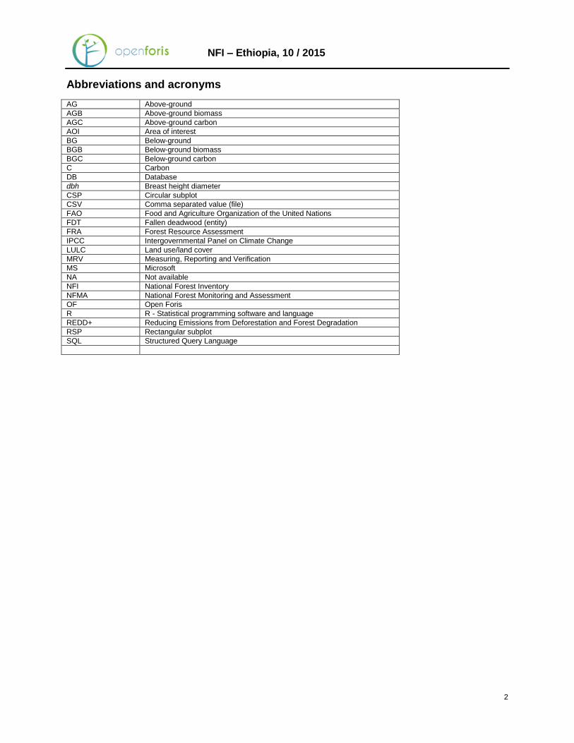
Abbreviations and acronyms
AG Above-ground
AGB Above-ground biomass
AGC Above-ground carbon
AOI Area of interest
BG Below-ground
BGB Below-ground biomass
BGC Below-ground carbon
C Carbon
DB Database
dbh Breast height diameter
CSP Circular subplot
CSV Comma separated value (file)
FAO Food and Agriculture Organization of the United Nations
FDT Fallen deadwood (entity)
FRA Forest Resource Assessment
IPCC Intergovernmental Panel on Climate Change
LULC Land use/land cover
MRV Measuring, Reporting and Verification
MS Microsoft
NA Not available
NFI National Forest Inventory
NFMA National Forest Monitoring and Assessment
OF Open Foris
R R - Statistical programming software and language
REDD+ Reducing Emissions from Deforestation and Forest Degradation
RSP Rectangular subplot
SQL Structured Query Language
3
NFI – Ethiopia, 10 / 2015
PREFACE
Open Foris (OF) Calc is a robust, modular browser-based tool for data analysis and results calculation. It allows expert users to write custom R modules to perform country/inventory-specific calculations. This document contains brief description of these modules written in the context of the “Implementation of a National Forest Monitoring and MRV system for REDD+ readiness in Ethiopia” project (UTF/086/ETH). NFI sampling design is based on stratified systematic sampling, where the whole country is divided into four strata. These strata are as follows: 1) High altitude (where Afroalpine and Montain forest are dominated), 2) Middle altitude (where most of human activities are dominated and evergreen dry mountain forests are existed), 3) Hot low lands (where most of Ethiopian Woodland dominated and mostly found to the west and eastern part of the country, Termilania combretum and Acacia comifora woodland existed, respectively), and 4) Desert/Arid area (where most scrub and bare land dominated ecosystems is prevalent). The area estimates for strata are taken from the inventory design. In OF Calc, the areas of strata are given in as hectares by strata, and in the program we need to apply the cluster sampling method. The input data structure (i.e. metadata) and variable names come from Open Foris Collect database. In the NFI sample plot design a cluster (i.e. sampling unit) consists of four sample plots. Each sample plot can be divides into land use/land cover (LULC) sections. Trees and stumps are recorded in the whole plot area, and small trees (in forest) and saplings are recorded in smaller subplots. The plot design causes that there is not equal sampling probability for trees and small trees in the sub-plots (in terms of land use/vegetation types), so in computing the results we must apply two different areal weighting methods for tree and sapling data. Fallen deadwood data is a special case because this data is collected using a transect line sampling method. So, the OF workspace is made for computing results for all entities, but only results for trees, stumps, and removal can be reported using Saiku. The results for saplings (dbh< 10cm) and fallen deadwood are written into csv-files. Calc and Saiku provide a flexible way to produce aggregated results. The aggregated results can be analyzed and visualized through open-source software Saiku, or exported from Calc or Saiku e.g. to MS Excel or R for further analysis. Allometric models, calculation chains and individual calculation modules will be further developed in Ethiopia, so these scripts may meet some changes in the future. However, this document aims to show the current progress, and hopefully it also works as a model when tailoring Calc into forest inventories in other countries which have applied FAO’s “traditional” National Forest Monitoring and Assessment (NFMA) sampling approach.
This Open Foris Calc code contains some outputs that are written into CSV format files into a predefined folder set into variable 'ResultFolder’, see for example the script of the calculation module 3.1 “Trees (dbh<10cm) ->CSV“. This is done because all results cannot be shown using Saiku. Therefore this output folder must exist in the computer where Calc is run.
4
NFI – Ethiopia, 10 / 2015
1. PRINCIPLES OF DATA PROCESSING
1.1. Reporting levels
NFI is following the stratified systematic sampling and the results need to be analysed by stratums. The results for Ethiopian NFI are computed for the following reporting levels (i.e. areas):
1. Country (level 1 in AOI table), 2. Region (level 2 in AOI table), 3. Stratum (level 3 in AOI table), 4. FAO-FRA class, 5. Vegetation type
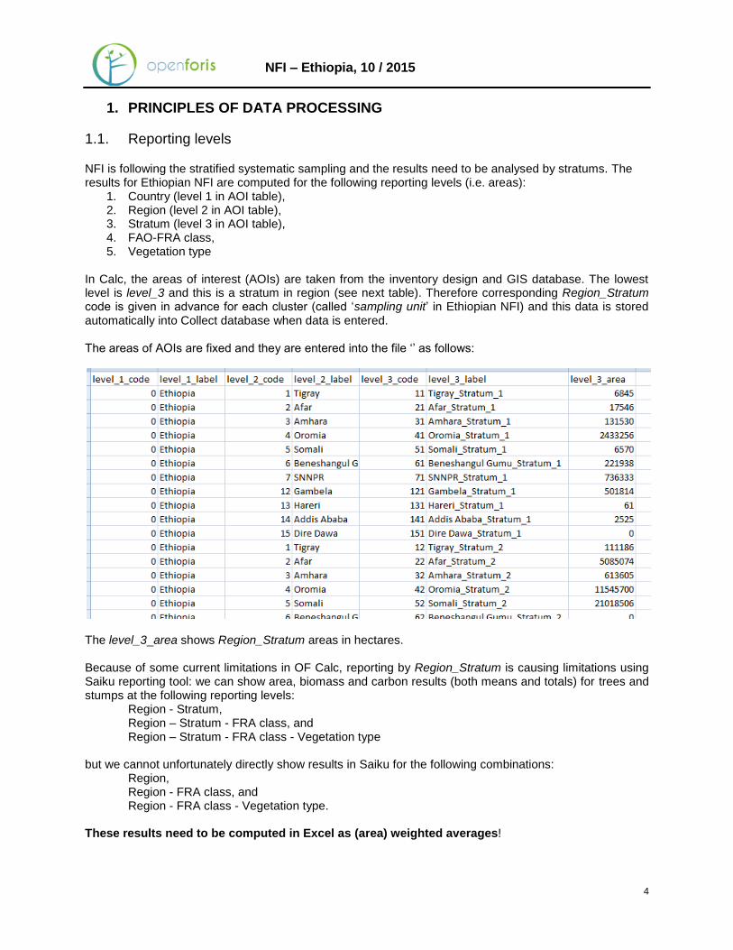
In Calc, the areas of interest (AOIs) are taken from the inventory design and GIS database. The lowest level is level_3 and this is a stratum in region (see next table). Therefore corresponding Region_Stratum code is given in advance for each cluster (called ‘sampling unit’ in Ethiopian NFI) and this data is stored automatically into Collect database when data is entered. The areas of AOIs are fixed and they are entered into the file ‘’ as follows:
The level_3_area shows Region_Stratum areas in hectares. Because of some current limitations in OF Calc, reporting by Region_Stratum is causing limitations using Saiku reporting tool: we can show area, biomass and carbon results (both means and totals) for trees and stumps at the following reporting levels:
Region - Stratum, Region – Stratum - FRA class, and Region – Stratum - FRA class - Vegetation type
but we cannot unfortunately directly show results in Saiku for the following combinations:
Region, Region - FRA class, and Region - FRA class - Vegetation type.
These results need to be computed in Excel as (area) weighted averages!
5
NFI – Ethiopia, 10 / 2015
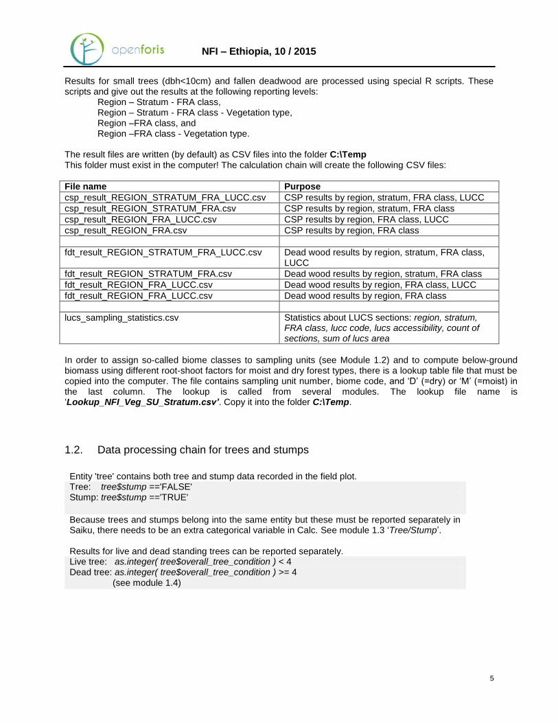
Results for small trees (dbh<10cm) and fallen deadwood are processed using special R scripts. These scripts and give out the results at the following reporting levels:
Region – Stratum - FRA class, Region – Stratum - FRA class - Vegetation type, Region –FRA class, and Region –FRA class - Vegetation type.
The result files are written (by default) as CSV files into the folder C:\Temp This folder must exist in the computer! The calculation chain will create the following CSV files:
File name Purpose
csp_result_REGION_STRATUM_FRA_LUCC.csv CSP results by region, stratum, FRA class, LUCC
csp_result_REGION_STRATUM_FRA.csv CSP results by region, stratum, FRA class
csp_result_REGION_FRA_LUCC.csv CSP results by region, FRA class, LUCC
csp_result_REGION_FRA.csv CSP results by region, FRA class
fdt_result_REGION_STRATUM_FRA_LUCC.csv Dead wood results by region, stratum, FRA class, LUCC
fdt_result_REGION_STRATUM_FRA.csv Dead wood results by region, stratum, FRA class
fdt_result_REGION_FRA_LUCC.csv Dead wood results by region, FRA class, LUCC
fdt_result_REGION_FRA_LUCC.csv Dead wood results by region, FRA class
lucs_sampling_statistics.csv Statistics about LUCS sections: region, stratum, FRA class, lucc code, lucs accessibility, count of sections, sum of lucs area
In order to assign so-called biome classes to sampling units (see Module 1.2) and to compute below-ground biomass using different root-shoot factors for moist and dry forest types, there is a lookup table file that must be copied into the computer. The file contains sampling unit number, biome code, and ‘D’ (=dry) or ‘M’ (=moist) in the last column. The lookup is called from several modules. The lookup file name is ‘Lookup_NFI_Veg_SU_Stratum.csv’. Copy it into the folder C:\Temp.
1.2. Data processing chain for trees and stumps
Entity 'tree' contains both tree and stump data recorded in the field plot. Tree: tree$stump =='FALSE' Stump: tree$stump =='TRUE'
Because trees and stumps belong into the same entity but these must be reported separately in Saiku, there needs to be an extra categorical variable in Calc. See module 1.3 ‘Tree/Stump’. Results for live and dead standing trees can be reported separately. Live tree: as.integer( tree$overall_tree_condition ) < 4 Dead tree: as.integer( tree$overall_tree_condition ) >= 4 (see module 1.4)
6
NFI – Ethiopia, 10 / 2015
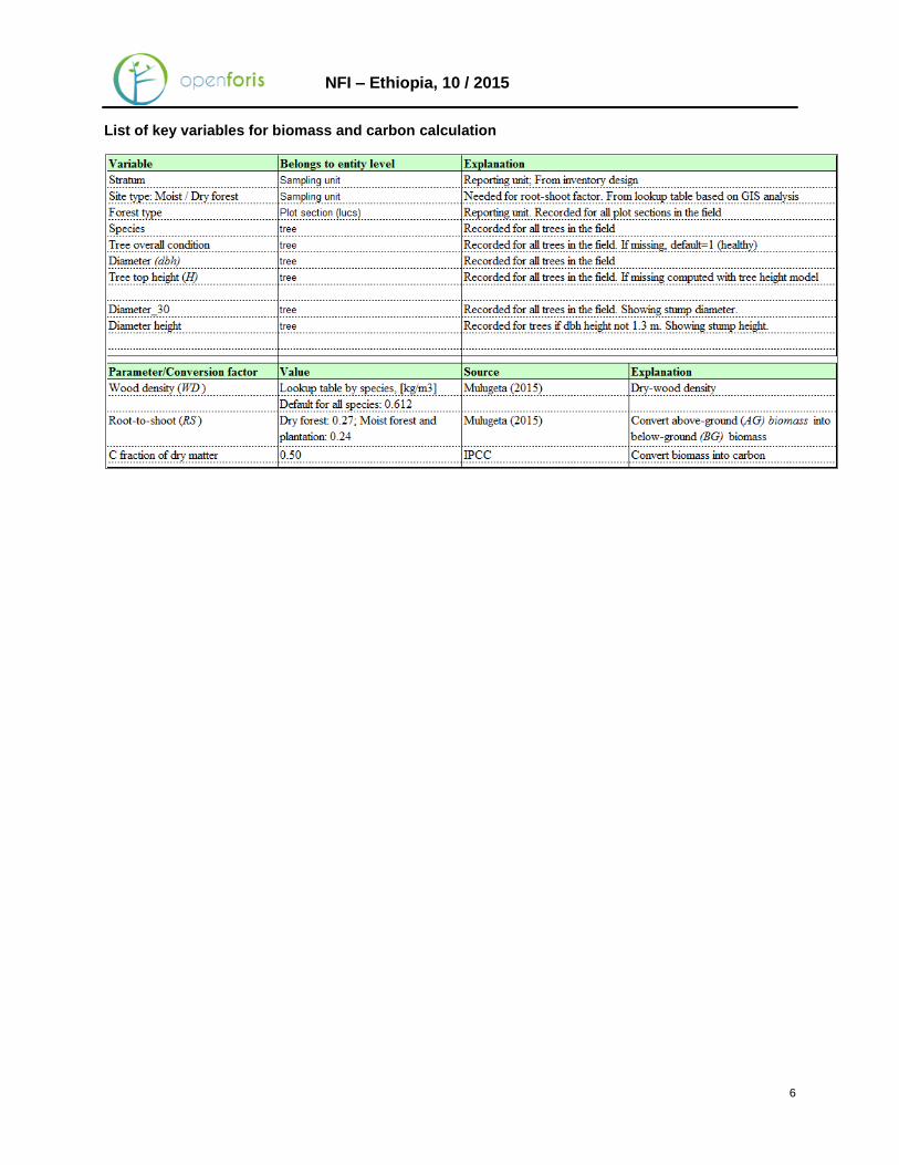
List of key variables for biomass and carbon calculation
7
NFI – Ethiopia, 10 / 2015
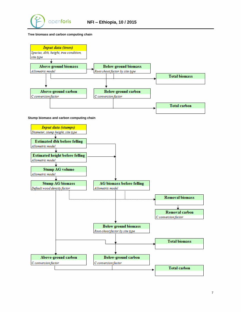
Tree biomass and carbon computing chain
Stump biomass and carbon computing chain
8
NFI – Ethiopia, 10 / 2015
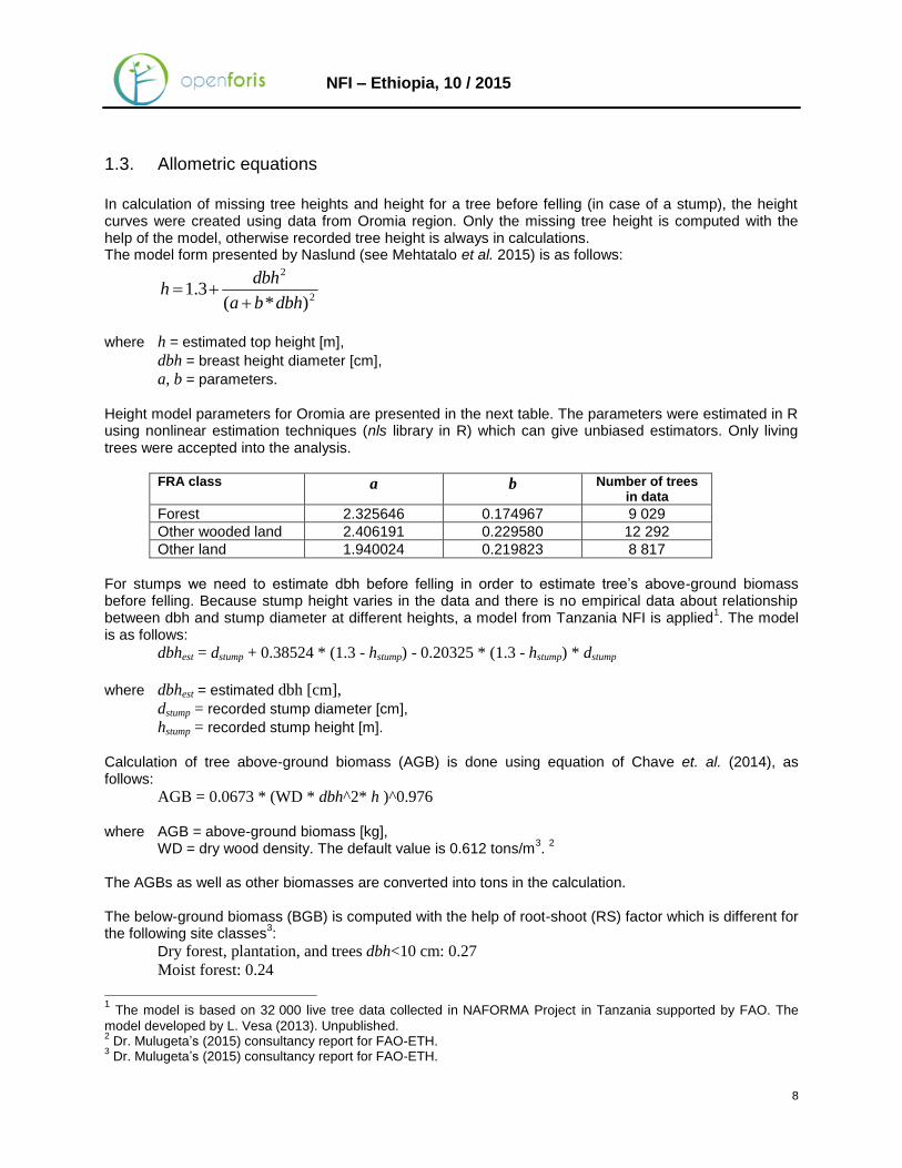
1.3. Allometric equations
In calculation of missing tree heights and height for a tree before felling (in case of a stump), the height curves were created using data from Oromia region. Only the missing tree height is computed with the help of the model, otherwise recorded tree height is always in calculations. The model form presented by Naslund (see Mehtatalo et al. 2015) is as follows:
2
2
)*(3.1
dbhba
dbhh
where h = estimated top height [m],
dbh = breast height diameter [cm],
a, b = parameters.
Height model parameters for Oromia are presented in the next table. The parameters were estimated in R using nonlinear estimation techniques (nls library in R) which can give unbiased estimators. Only living trees were accepted into the analysis.
FRA class a b Number of trees
in data
Forest 2.325646 0.174967 9 029
Other wooded land 2.406191 0.229580 12 292
Other land 1.940024 0.219823 8 817
For stumps we need to estimate dbh before felling in order to estimate tree’s above-ground biomass before felling. Because stump height varies in the data and there is no empirical data about relationship between dbh and stump diameter at different heights, a model from Tanzania NFI is applied
1. The model
is as follows:
dbhest = dstump + 0.38524 * (1.3 - hstump) - 0.20325 * (1.3 - hstump) * dstump
where dbhest = estimated dbh [cm],
dstump = recorded stump diameter [cm],
hstump = recorded stump height [m].
Calculation of tree above-ground biomass (AGB) is done using equation of Chave et. al. (2014), as follows:
AGB = 0.0673 * (WD * dbh^2* h )^0.976 where AGB = above-ground biomass [kg], WD = dry wood density. The default value is 0.612 tons/m
3.
2
The AGBs as well as other biomasses are converted into tons in the calculation. The below-ground biomass (BGB) is computed with the help of root-shoot (RS) factor which is different for the following site classes
3:
Dry forest, plantation, and trees dbh<10 cm: 0.27
Moist forest: 0.24
1 The model is based on 32 000 live tree data collected in NAFORMA Project in Tanzania supported by FAO. The
model developed by L. Vesa (2013). Unpublished. 2 Dr. Mulugeta’s (2015) consultancy report for FAO-ETH.
3 Dr. Mulugeta’s (2015) consultancy report for FAO-ETH.
9
NFI – Ethiopia, 10 / 2015
In the calculation there is a lookup table (see chapter 1.1.) for each sampling unit (SU, i.e. cluster) showing clusters falling into corresponding site category. The stump above-ground volume is computed as cylinder based on recorded stump’s diameter and height, and stump’s above-ground biomass (i.e. AG biomass remaining in the land) is computed with the help of default WD factor. The default carbon fraction to convert biomass into carbon is 0.50.
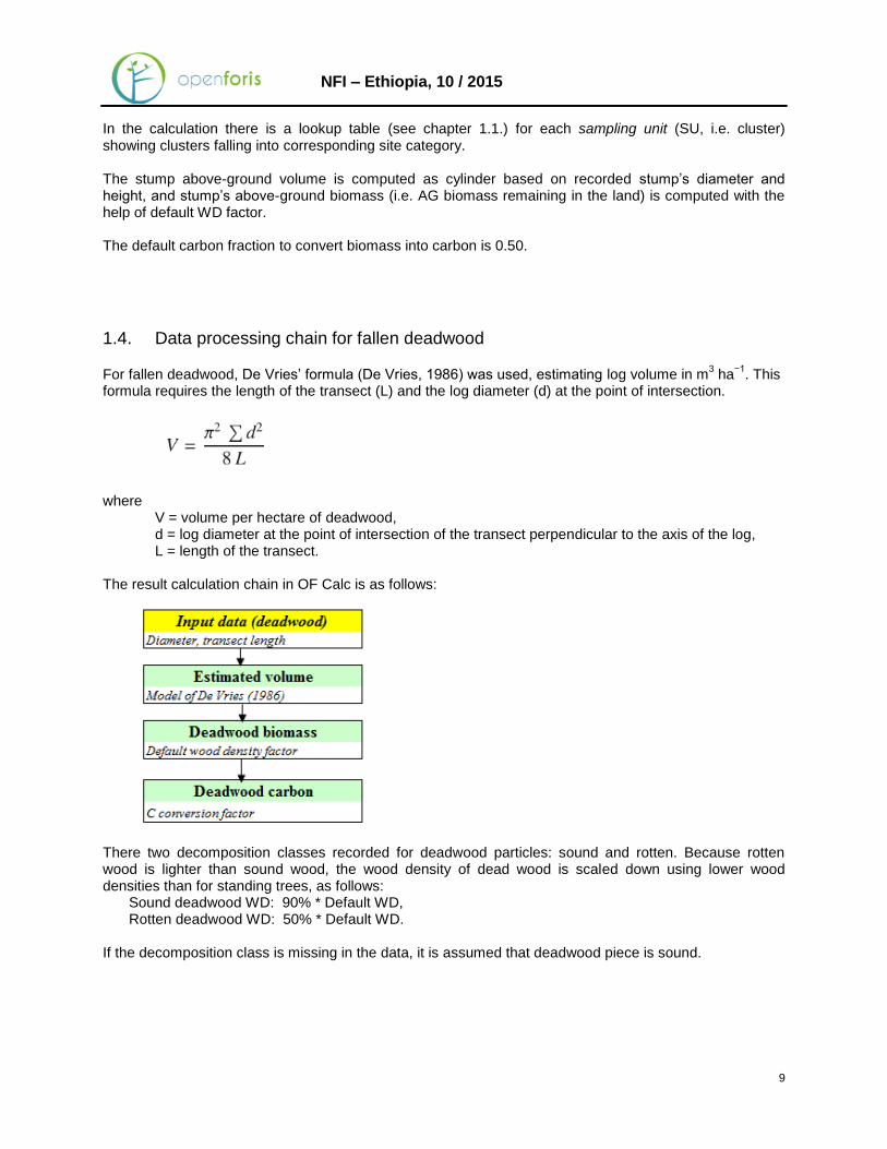
1.4. Data processing chain for fallen deadwood
For fallen deadwood, De Vries’ formula (De Vries, 1986) was used, estimating log volume in m3 ha
−1. This
formula requires the length of the transect (L) and the log diameter (d) at the point of intersection.
where
V = volume per hectare of deadwood, d = log diameter at the point of intersection of the transect perpendicular to the axis of the log, L = length of the transect.
The result calculation chain in OF Calc is as follows:
There two decomposition classes recorded for deadwood particles: sound and rotten. Because rotten wood is lighter than sound wood, the wood density of dead wood is scaled down using lower wood densities than for standing trees, as follows:
Sound deadwood WD: 90% * Default WD, Rotten deadwood WD: 50% * Default WD.
If the decomposition class is missing in the data, it is assumed that deadwood piece is sound.
10
NFI – Ethiopia, 10 / 2015
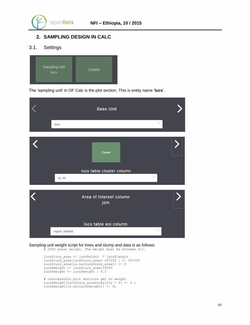
2. SAMPLING DESIGN IN CALC
3.1. Settings
The ‘sampling unit’ in OF Calc is the plot section. This is entity name ‘lucs’.
Sampling unit weight script for trees and stump and data is as follows: # LUCS areal weight. The weight must be between 0-1.
lucs$lucs_area <- lucs$width * lucs$length
lucs$lucs_area[lucs$lucs_area> 20*250 ] <- 20*250
lucs$lucs_area[is.na(lucs$lucs_area)] <- 0
lucs$weight <- lucs$lucs_area/10000
lucs$weight <- lucs$weight / 0.5
# inaccessible plot sections get no weight
lucs$weight[lucs$lucs_accessibility > 0] <- 0 ;
lucs$weight[is.na(lucs$weight)] <- 0;
11
NFI – Ethiopia, 10 / 2015
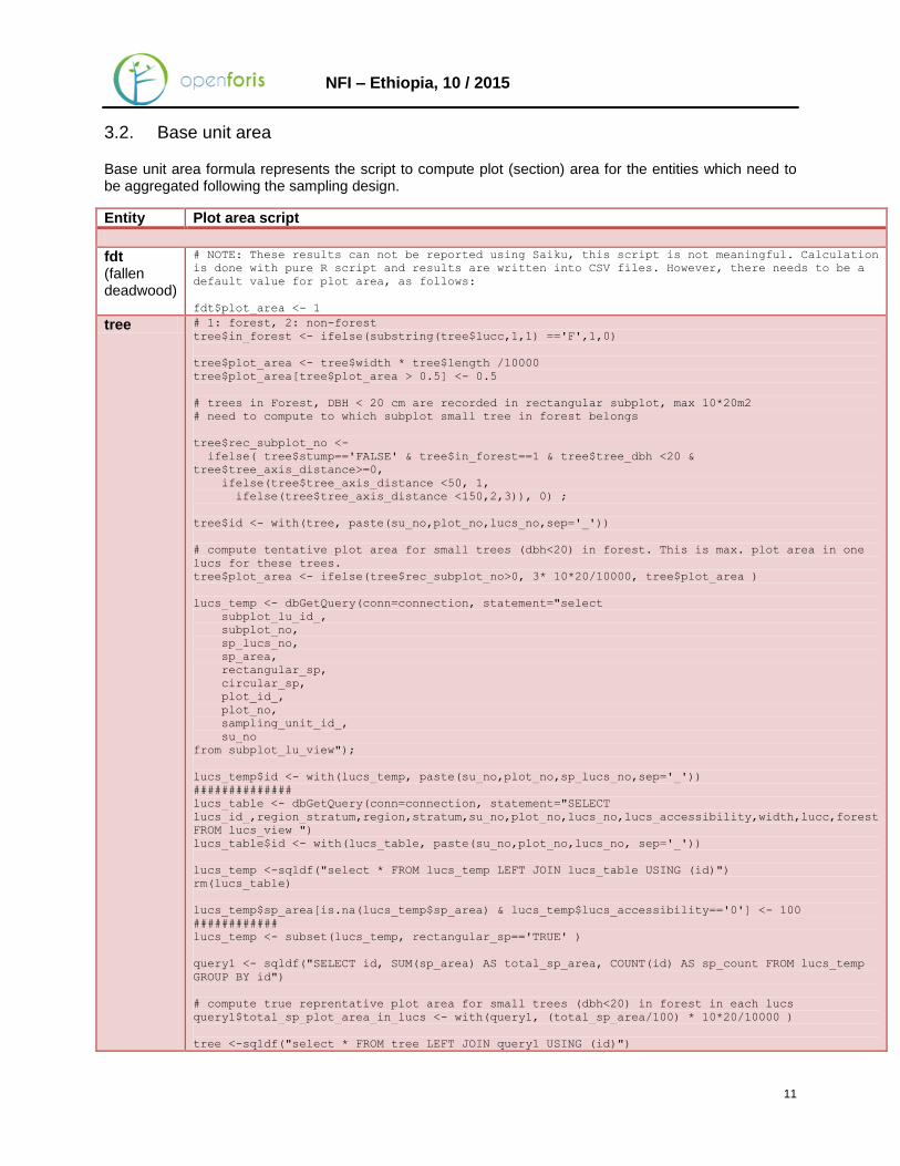
3.2. Base unit area
Base unit area formula represents the script to compute plot (section) area for the entities which need to be aggregated following the sampling design.
Entity Plot area script
fdt (fallen deadwood)
# NOTE: These results can not be reported using Saiku, this script is not meaningful. Calculation
is done with pure R script and results are written into CSV files. However, there needs to be a
default value for plot area, as follows:
fdt$plot_area <- 1
tree # 1: forest, 2: non-forest
tree$in_forest <- ifelse(substring(tree$lucc,1,1) =='F',1,0)
tree$plot_area <- tree$width * tree$length /10000
tree$plot_area[tree$plot_area > 0.5] <- 0.5
# trees in Forest, DBH < 20 cm are recorded in rectangular subplot, max 10*20m2
# need to compute to which subplot small tree in forest belongs
tree$rec_subplot_no <-
ifelse( tree$stump=='FALSE' & tree$in_forest==1 & tree$tree_dbh <20 &
tree$tree_axis_distance>=0,
ifelse(tree$tree_axis_distance <50, 1,
ifelse(tree$tree_axis_distance <150,2,3)), 0) ;
tree$id <- with(tree, paste(su_no,plot_no,lucs_no,sep='_'))
# compute tentative plot area for small trees (dbh<20) in forest. This is max. plot area in one
lucs for these trees.
tree$plot_area <- ifelse(tree$rec_subplot_no>0, 3* 10*20/10000, tree$plot_area )
lucs_temp <- dbGetQuery(conn=connection, statement="select
subplot_lu_id_,
subplot_no,
sp_lucs_no,
sp_area,
rectangular_sp,
circular_sp,
plot_id_,
plot_no,
sampling_unit_id_,
su_no
from subplot_lu_view");
lucs_temp$id <- with(lucs_temp, paste(su_no,plot_no,sp_lucs_no,sep='_'))
##############
lucs_table <- dbGetQuery(conn=connection, statement="SELECT
lucs_id_,region_stratum,region,stratum,su_no,plot_no,lucs_no,lucs_accessibility,width,lucc,forest
FROM lucs_view ")
lucs_table$id <- with(lucs_table, paste(su_no,plot_no,lucs_no, sep='_'))
lucs_temp <-sqldf("select * FROM lucs_temp LEFT JOIN lucs_table USING (id)")
rm(lucs_table)
lucs_temp$sp_area[is.na(lucs_temp$sp_area) & lucs_temp$lucs_accessibility=='0'] <- 100
############
lucs_temp <- subset(lucs_temp, rectangular_sp=='TRUE' )
query1 <- sqldf("SELECT id, SUM(sp_area) AS total_sp_area, COUNT(id) AS sp_count FROM lucs_temp
GROUP BY id")
# compute true reprentative plot area for small trees (dbh<20) in forest in each lucs
query1$total_sp_plot_area_in_lucs <- with(query1, (total_sp_area/100) * 10*20/10000 )
tree <-sqldf("select * FROM tree LEFT JOIN query1 USING (id)")

12
NFI – Ethiopia, 10 / 2015
rm(lucs_temp)
rm(query1)
# replace tentative subplot area with true value in lucs (=plot section) for small tree in forest
tree$plot_area <- ifelse(tree$rec_subplot_no>0 & tree$total_sp_plot_area_in_lucs>0 &
tree$total_sp_plot_area_in_lucs < tree$plot_area,
tree$total_sp_plot_area_in_lucs, tree$plot_area )
13
NFI – Ethiopia, 10 / 2015
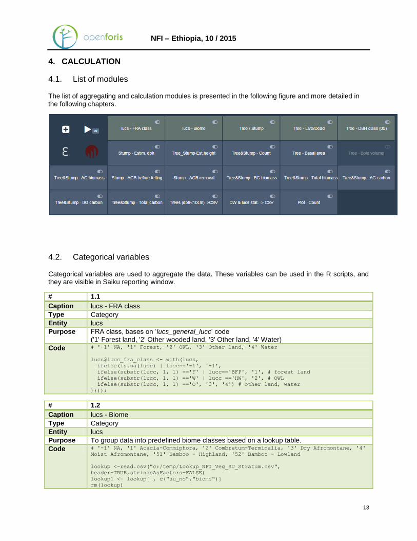
4. CALCULATION
4.1. List of modules
The list of aggregating and calculation modules is presented in the following figure and more detailed in the following chapters.
4.2. Categorical variables
Categorical variables are used to aggregate the data. These variables can be used in the R scripts, and they are visible in Saiku reporting window.
# 1.1
Caption lucs - FRA class
Type Category
Entity lucs
Purpose FRA class, bases on ‘lucs_general_lucc’ code ('1' Forest land, '2' Other wooded land, '3' Other land, '4' Water)
Code # '-1' NA, '1' Forest, '2' OWL, '3' Other land, '4' Water
lucs$lucs_fra_class <- with(lucs,
ifelse(is.na(lucc) | lucc=='-1', '-1',
ifelse(substr(lucc, 1, 1) =='F' | lucc=='BFP', '1', # forest land
ifelse(substr(lucc, 1, 1) =='W' | lucc =='HW', '2', # OWL
ifelse(substr(lucc, 1, 1) =='O', '3', '4') # other land, water
))));
# 1.2
Caption lucs - Biome
Type Category
Entity lucs
Purpose To group data into predefined biome classes based on a lookup table.
Code # '-1' NA, '1' Acacia-Commiphora, '2' Combretum-Terminalia, '3' Dry Afromontane, '4'
Moist Afromontane, '51' Bamboo - Highland, '52' Bamboo - Lowland
lookup <-read.csv("c:/temp/Lookup_NFI_Veg_SU_Stratum.csv",
header=TRUE,stringsAsFactors=FALSE)
lookup1 <- lookup[ , c("su_no","biome")]
rm(lookup)
14
NFI – Ethiopia, 10 / 2015
# join lookup showing biome
lucs <-sqldf("SELECT * FROM lucs LEFT JOIN lookup1 USING (su_no) ")
lucs$lucs_biome <- as.character(lucs$biome)
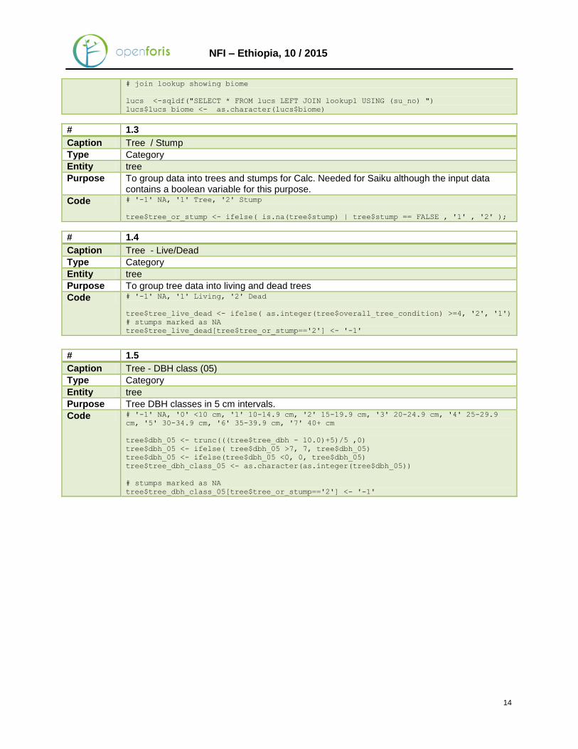
# 1.3
Caption Tree / Stump
Type Category
Entity tree
Purpose To group data into trees and stumps for Calc. Needed for Saiku although the input data contains a boolean variable for this purpose.
Code # '-1' NA, '1' Tree, '2' Stump
tree$tree_or_stump <- ifelse( is.na(tree$stump) | tree$stump == FALSE , '1' , '2' );
# 1.4
Caption Tree - Live/Dead
Type Category
Entity tree
Purpose To group tree data into living and dead trees
Code # '-1' NA, '1' Living, '2' Dead
tree$tree_live_dead <- ifelse( as.integer(tree$overall_tree_condition) >=4, '2', '1')
# stumps marked as NA
tree$tree_live_dead[tree$tree_or_stump=='2'] <- '-1'
# 1.5
Caption Tree - DBH class (05)
Type Category
Entity tree
Purpose Tree DBH classes in 5 cm intervals.
Code # '-1' NA, '0' <10 cm, '1' 10-14.9 cm, '2' 15-19.9 cm, '3' 20-24.9 cm, '4' 25-29.9
cm, '5' 30-34.9 cm, '6' 35-39.9 cm, '7' 40+ cm
tree$dbh_05 <- trunc(((tree$tree_dbh - 10.0)+5)/5 ,0)
tree$dbh_05 <- ifelse( tree$dbh_05 >7, 7, tree$dbh_05)
tree$dbh_05 <- ifelse(tree$dbh_05 <0, 0, tree$dbh_05)
tree$tree_dbh_class_05 <- as.character(as.integer(tree$dbh_05))
# stumps marked as NA
tree$tree_dbh_class_05[tree$tree_or_stump=='2'] <- '-1'
15
NFI – Ethiopia, 10 / 2015
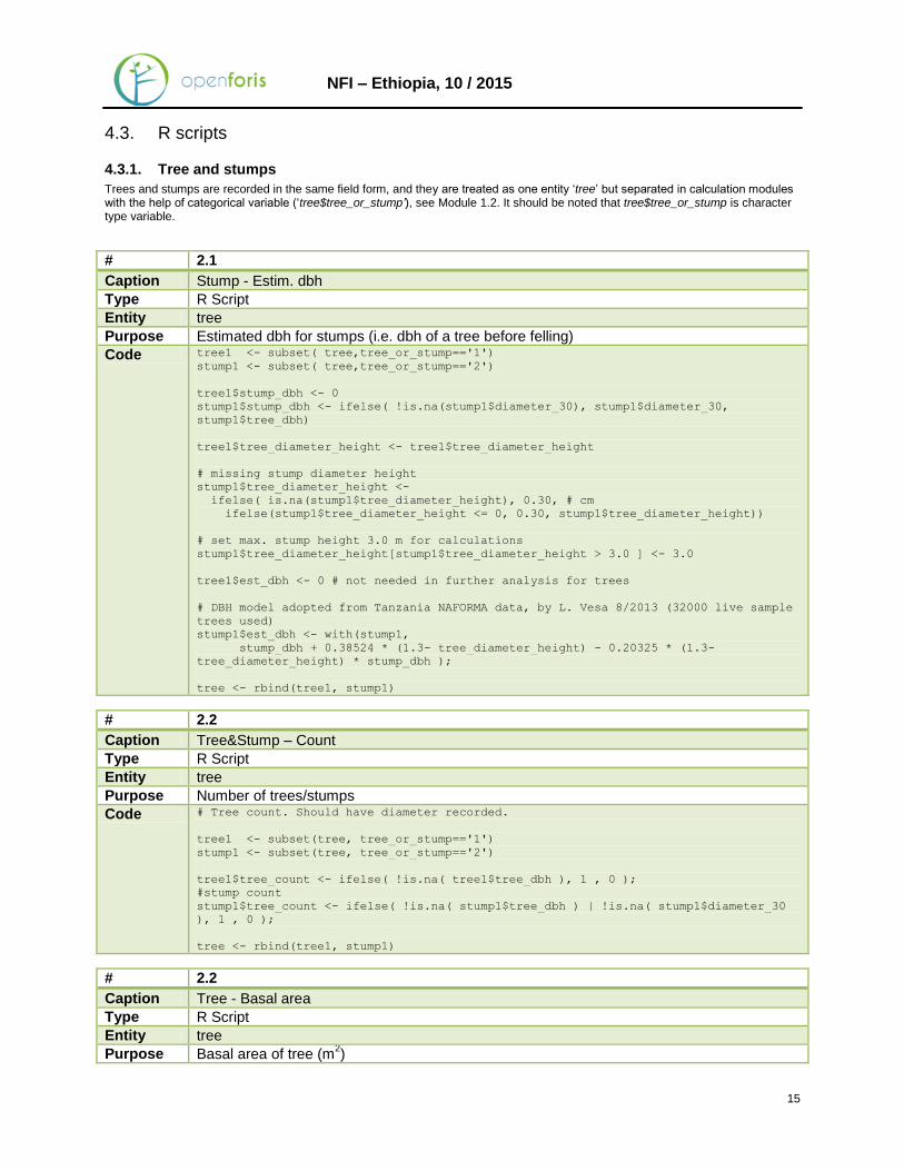
4.3. R scripts
4.3.1. Tree and stumps
Trees and stumps are recorded in the same field form, and they are treated as one entity ‘tree’ but separated in calculation modules with the help of categorical variable (‘tree$tree_or_stump’), see Module 1.2. It should be noted that tree$tree_or_stump is character type variable.
# 2.1
Caption Stump - Estim. dbh
Type R Script
Entity tree
Purpose Estimated dbh for stumps (i.e. dbh of a tree before felling)
Code tree1 <- subset( tree,tree_or_stump=='1')
stump1 <- subset( tree,tree_or_stump=='2')
tree1$stump_dbh <- 0
stump1$stump_dbh <- ifelse( !is.na(stump1$diameter_30), stump1$diameter_30,
stump1$tree_dbh)
tree1$tree_diameter_height <- tree1$tree_diameter_height
# missing stump diameter height
stump1$tree_diameter_height <-
ifelse( is.na(stump1$tree_diameter_height), 0.30, # cm
ifelse(stump1$tree_diameter_height <= 0, 0.30, stump1$tree_diameter_height))
# set max. stump height 3.0 m for calculations
stump1$tree_diameter_height[stump1$tree_diameter_height > 3.0 ] <- 3.0
tree1$est_dbh <- 0 # not needed in further analysis for trees
# DBH model adopted from Tanzania NAFORMA data, by L. Vesa 8/2013 (32000 live sample
trees used)
stump1$est_dbh <- with(stump1,
stump_dbh + 0.38524 * (1.3- tree_diameter_height) - 0.20325 * (1.3-
tree_diameter_height) * stump_dbh );
tree <- rbind(tree1, stump1)
# 2.2
Caption Tree&Stump – Count
Type R Script
Entity tree
Purpose Number of trees/stumps
Code # Tree count. Should have diameter recorded.
tree1 <- subset(tree, tree_or_stump=='1')
stump1 <- subset(tree, tree_or_stump=='2')
tree1$tree_count <- ifelse( !is.na( tree1$tree_dbh ), 1 , 0 );
#stump count
stump1$tree_count <- ifelse( !is.na( stump1$tree_dbh ) | !is.na( stump1$diameter_30
), 1 , 0 );
tree <- rbind(tree1, stump1)
# 2.2
Caption Tree - Basal area
Type R Script
Entity tree
Purpose Basal area of tree (m2)
16
NFI – Ethiopia, 10 / 2015
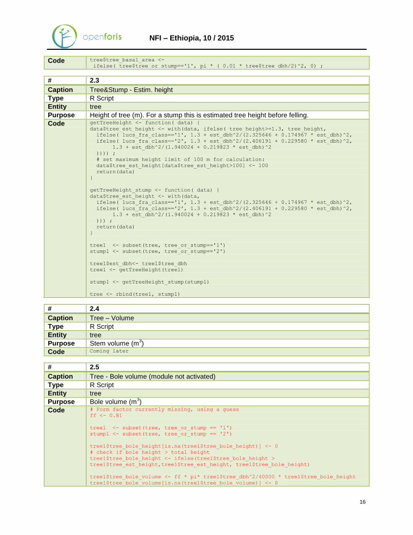
Code tree$tree_basal_area <-
ifelse( tree$tree_or_stump=='1', pi * ( 0.01 * tree$tree_dbh/2)^2, 0) ;
# 2.3
Caption Tree&Stump - Estim. height
Type R Script
Entity tree
Purpose Height of tree (m). For a stump this is estimated tree height before felling.
Code getTreeHeight <- function( data) {
data$tree_est_height <- with(data, ifelse( tree_height>=1.3, tree_height,
ifelse( lucs_fra_class=='1', 1.3 + est_dbh^2/(2.325646 + 0.174967 * est_dbh)^2,
ifelse( lucs_fra_class=='2', 1.3 + est_dbh^2/(2.406191 + 0.229580 * est_dbh)^2,
1.3 + est_dbh^2/(1.940024 + 0.219823 * est_dbh)^2
)))) ;
# set maximum height limit of 100 m for calculation:
data$tree_est_height[data$tree_est_height>100] <- 100
return(data)
}
getTreeHeight_stump <- function( data) {
data$tree_est_height <- with(data,
ifelse( lucs_fra_class=='1', 1.3 + est_dbh^2/(2.325646 + 0.174967 * est_dbh)^2,
ifelse( lucs_fra_class=='2', 1.3 + est_dbh^2/(2.406191 + 0.229580 * est_dbh)^2,
1.3 + est_dbh^2/(1.940024 + 0.219823 * est_dbh)^2
))) ;
return(data)
}
tree1 <- subset(tree, tree_or_stump=='1')
stump1 <- subset(tree, tree_or_stump=='2')
tree1$est_dbh<- tree1$tree_dbh
tree1 <- getTreeHeight(tree1)
stump1 <- getTreeHeight_stump(stump1)
tree <- rbind(tree1, stump1)
# 2.4
Caption Tree – Volume
Type R Script
Entity tree
Purpose Stem volume (m3)
Code Coming later
# 2.5
Caption Tree - Bole volume (module not activated)
Type R Script
Entity tree
Purpose Bole volume (m3)
Code # Form factor currently missing, using a guess
ff <- 0.81
tree1 <- subset(tree, tree_or_stump == '1')
stump1 <- subset(tree, tree_or_stump == '2')
tree1$tree_bole_height[is.na(tree1$tree_bole_height)] <- 0
# check if bole height > total height
tree1$tree_bole_height <- ifelse(tree1$tree_bole_height >
tree1$tree_est_height,tree1$tree_est_height, tree1$tree_bole_height)
tree1$tree_bole_volume <- ff * pi* tree1$tree_dbh^2/40000 * tree1$tree_bole_height
tree1$tree_bole_volume[is.na(tree1$tree_bole_volume)] <- 0

17
NFI – Ethiopia, 10 / 2015
stump1$tree_bole_volume <- NA
tree <- rbind(tree1, stump1)
# 2.6
Caption Tree&Stump - AG biomass
Type R Script
Entity tree
Purpose Above-ground biomass (tons)
Code # default Dry Wood Density (Mulugeta 2015)
wd <- 0.612
tree1 <- subset(tree, tree_or_stump == '1')
stump1 <- subset(tree, tree_or_stump == '2')
# model source: Chave et al. 2014
tree1$tree_ag_biomass <- 0.0673*( wd * tree1$tree_dbh^2 * tree1$tree_est_height
)^0.976
# convert kg -> tons
tree1$tree_ag_biomass <- tree1$tree_ag_biomass / 1000
tree1$stump_diameter <- NA
tree1$stump_height <- NA
tree1$stump_volume <- NA
stump1$stump_diameter <- ifelse(!is.na(stump1$diameter_30), stump1$diameter_30,
stump1$tree_dbh)
stump1$stump_height <- ifelse(!is.na(stump1$tree_diameter_height),
stump1$tree_diameter_height, stump1$tree_height)
#set max stump height to 3 m
stump1$stump_height[stump1$stump_height>3.0] <- 3.0
stump1$stump_volume <- pi*stump1$stump_diameter^2/40000 * stump1$stump_height
stump1$tree_ag_biomass <- stump1$stump_volume * wd
tree <- rbind(tree1, stump1)
# 2.7
Caption Stump - AGB before felling
Type R Script
Entity tree
Purpose Above-ground biomass before felling (tons)
Code # default Dry Wood Density (Mulugeta 2015)
wd <- 0.612
tree1 <- subset(tree, tree_or_stump == '1')
stump1 <- subset(tree, tree_or_stump == '2')
tree1$stump_agb_before_felling <- NA
# model source: Chave et al. 2014
stump1$stump_agb_before_felling <- 0.0673*( wd * stump1$est_dbh^2 *
stump1$tree_est_height )^0.976
# convert kg -> tons
stump1$stump_agb_before_felling <- stump1$stump_agb_before_felling / 1000
tree <- rbind(tree1, stump1)
# 2.8
Caption Stump - AGB removal
Type R Script
Entity tree
Purpose Above-ground removal due to felling (tons)
Code tree1 <- subset(tree, tree_or_stump == '1')
stump1 <- subset(tree, tree_or_stump == '2')
18
NFI – Ethiopia, 10 / 2015
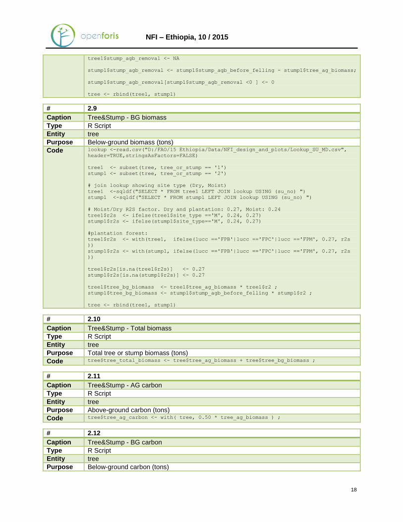
tree1$stump_agb_removal <- NA
stump1$stump_agb_removal <- stump1$stump_agb_before_felling - stump1$tree_ag_biomass;
stump1$stump_agb_removal[stump1$stump_agb_removal <0 ] <- 0
tree <- rbind(tree1, stump1)
# 2.9
Caption Tree&Stump - BG biomass
Type R Script
Entity tree
Purpose Below-ground biomass (tons)
Code lookup <-read.csv("D:/FAO/15 Ethiopia/Data/NFI_design_and_plots/Lookup_SU_MD.csv",
header=TRUE,stringsAsFactors=FALSE)
tree1 <- subset(tree, tree_or_stump == '1')
stump1 <- subset(tree, tree_or_stump == '2')
# join lookup showing site type (Dry, Moist)
tree1 <-sqldf("SELECT * FROM tree1 LEFT JOIN lookup USING (su_no) ")
stump1 <-sqldf("SELECT * FROM stump1 LEFT JOIN lookup USING (su_no) ")
# Moist/Dry R2S factor. Dry and plantation: 0.27, Moist: 0.24
tree1$r2s <- ifelse(tree1$site_type =='M', 0.24, 0.27)
stump1$r2s <- ifelse(stump1$site_type=='M', 0.24, 0.27)
#plantation forest:
tree1$r2s <- with(tree1, ifelse(lucc =='FPB'|lucc =='FPC'|lucc =='FPM', 0.27, r2s
))
stump1$r2s <- with(stump1, ifelse(lucc =='FPB'|lucc =='FPC'|lucc =='FPM', 0.27, r2s
))
tree1$r2s[is.na(tree1$r2s)] <- 0.27
stump1$r2s[is.na(stump1$r2s)] <- 0.27
tree1$tree_bg_biomass <- tree1$tree_ag_biomass * tree1$r2 ;
stump1$tree_bg_biomass <- stump1$stump_agb_before_felling * stump1$r2 ;
tree <- rbind(tree1, stump1)
# 2.10
Caption Tree&Stump - Total biomass
Type R Script
Entity tree
Purpose Total tree or stump biomass (tons)
Code tree$tree_total_biomass <- tree$tree_ag_biomass + tree$tree_bg_biomass ;
# 2.11
Caption Tree&Stump - AG carbon
Type R Script
Entity tree
Purpose Above-ground carbon (tons)
Code tree$tree_ag_carbon <- with( tree, 0.50 * tree_ag_biomass ) ;
# 2.12
Caption Tree&Stump - BG carbon
Type R Script
Entity tree
Purpose Below-ground carbon (tons)
19
NFI – Ethiopia, 10 / 2015
Code tree$tree_bg_carbon <- with(tree, 0.50 * tree_bg_biomass );
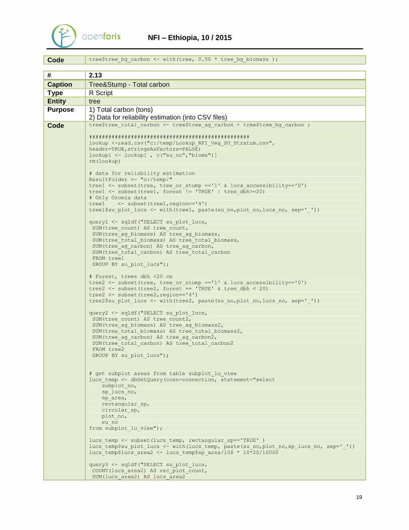
# 2.13
Caption Tree&Stump - Total carbon
Type R Script
Entity tree
Purpose 1) Total carbon (tons) 2) Data for reliability estimation (into CSV files)
Code tree$tree_total_carbon <- tree$tree_ag_carbon + tree$tree_bg_carbon ;
##################################################
lookup <-read.csv("c:/temp/Lookup_NFI_Veg_SU_Stratum.csv",
header=TRUE,stringsAsFactors=FALSE)
lookup1 <- lookup[ , c("su_no","biome")]
rm(lookup)
# data for reliability estimation
ResultFolder <- "c:/temp/"
tree1 <- subset(tree, tree_or_stump =='1' & lucs_accessibility=='0')
tree1 <- subset(tree1, forest != 'TRUE' | tree_dbh>=20)
# Only Oromia data
tree1 <- subset(tree1,region=='4')
tree1$su_plot_lucs <- with(tree1, paste(su_no,plot_no,lucs_no, sep='_'))
query1 <- sqldf("SELECT su_plot_lucs,
SUM(tree_count) AS tree_count,
SUM(tree_ag_biomass) AS tree_ag_biomass,
SUM(tree_total_biomass) AS tree_total_biomass,
SUM(tree_ag_carbon) AS tree_ag_carbon,
SUM(tree_total_carbon) AS tree_total_carbon
FROM tree1
GROUP BY su_plot_lucs");
# Forest, trees dbh <20 cm
tree2 <- subset(tree, tree_or_stump =='1' & lucs_accessibility=='0')
tree2 <- subset(tree2, forest == 'TRUE' & tree_dbh < 20)
tree2 <- subset(tree2,region=='4')
tree2$su_plot_lucs <- with(tree2, paste(su_no,plot_no,lucs_no, sep='_'))
query2 <- sqldf("SELECT su_plot_lucs,
SUM(tree_count) AS tree_count2,
SUM(tree_ag_biomass) AS tree_ag_biomass2,
SUM(tree_total_biomass) AS tree_total_biomass2,
SUM(tree_ag_carbon) AS tree_ag_carbon2,
SUM(tree_total_carbon) AS tree_total_carbon2
FROM tree2
GROUP BY su_plot_lucs");
# get subplot areas from table subplot_lu_view
lucs_temp <- dbGetQuery(conn=connection, statement="select
subplot_no,
sp_lucs_no,
sp_area,
rectangular_sp,
circular_sp,
plot_no,
su_no
from subplot_lu_view");
lucs_temp <- subset(lucs_temp, rectangular_sp=='TRUE' )
lucs_temp$su_plot_lucs <- with(lucs_temp, paste(su_no,plot_no,sp_lucs_no, sep='_'))
lucs_temp$lucs_area2 <- lucs_temp$sp_area/100 * 10*20/10000
query3 <- sqldf("SELECT su_plot_lucs,
COUNT(lucs_area2) AS rec_plot_count,
SUM(lucs_area2) AS lucs_area2
20
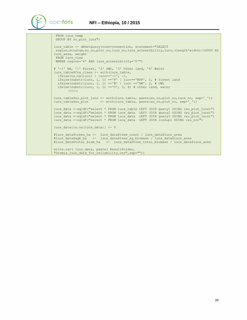
NFI – Ethiopia, 10 / 2015
FROM lucs_temp
GROUP BY su_plot_lucs")
lucs_table <- dbGetQuery(conn=connection, statement="SELECT
region,stratum,su_no,plot_no,lucs_no,lucs_accessibility,lucc,(length*width)/10000 AS
lucs_area, weight
FROM lucs_view
WHERE region='4' AND lucs_accessibility='0'")
# '-1' NA, '1' Forest, '2' OWL, '3' Other land, '4' Water
lucs_table$fra_class <- with(lucs_table,
ifelse(is.na(lucc) | lucc=='-1', -1,
ifelse(substr(lucc, 1, 1) =='F' | lucc=='BFP', 1, # forest land
ifelse(substr(lucc, 1, 1) =='W' | lucc =='HW', 2, # OWL
ifelse(substr(lucc, 1, 1) =='O', 3, 4) # other land, water
))));
lucs_table$su_plot_lucs <- with(lucs_table, paste(su_no,plot_no,lucs_no, sep='_'))
lucs_table$su_plot <- with(lucs_table, paste(su_no,plot_no, sep='_'))
lucs_data <-sqldf("select * FROM lucs_table LEFT JOIN query1 USING (su_plot_lucs)")
lucs_data <-sqldf("select * FROM lucs_data LEFT JOIN query2 USING (su_plot_lucs)")
lucs_data <-sqldf("select * FROM lucs_data LEFT JOIN query3 USING (su_plot_lucs)")
lucs_data <-sqldf("select * FROM lucs_data LEFT JOIN lookup1 USING (su_no)")
lucs_data[is.na(lucs_data)] <- 0
#lucs_data$trees_ha <- lucs_data$tree_count / lucs_data$lucs_area
#lucs_data$agb_ha <- lucs_data$tree_ag_biomass / lucs_data$lucs_area
#lucs_data$total_biom_ha <- lucs_data$tree_total_biomass / lucs_data$lucs_area
write.csv( lucs_data, paste( ResultFolder,
"Oromia_lucs_data_for_reliability.csv",sep=""))
21
NFI – Ethiopia, 10 / 2015
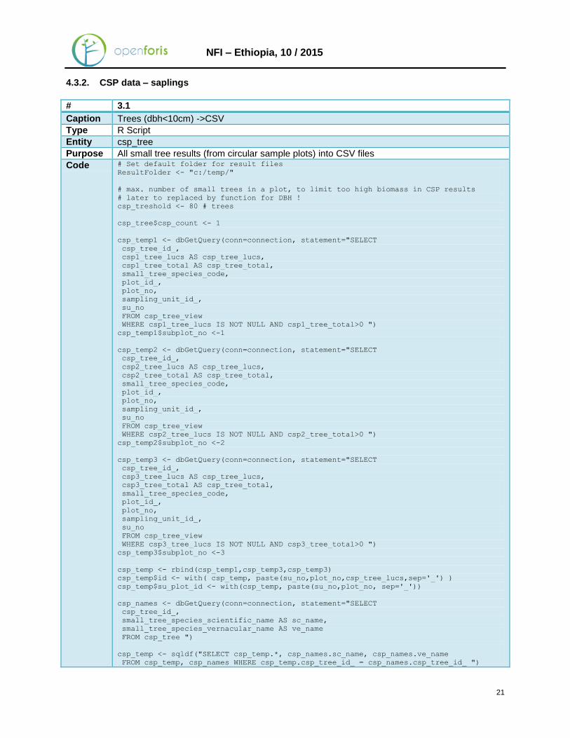
4.3.2. CSP data – saplings
# 3.1
Caption Trees (dbh<10cm) ->CSV
Type R Script
Entity csp_tree
Purpose All small tree results (from circular sample plots) into CSV files
Code # Set default folder for result files
ResultFolder <- "c:/temp/"
# max. number of small trees in a plot, to limit too high biomass in CSP results
# later to replaced by function for DBH !
csp_treshold <- 80 # trees
csp_tree$csp_count <- 1
csp_temp1 <- dbGetQuery(conn=connection, statement="SELECT
csp_tree_id_,
csp1_tree_lucs AS csp_tree_lucs,
csp1_tree_total AS csp_tree_total,
small_tree_species_code,
plot_id_,
plot_no,
sampling_unit_id_,
su_no
FROM csp_tree_view
WHERE csp1_tree_lucs IS NOT NULL AND csp1_tree_total>0 ")
csp_temp1$subplot_no <-1
csp_temp2 <- dbGetQuery(conn=connection, statement="SELECT
csp_tree_id_,
csp2_tree_lucs AS csp_tree_lucs,
csp2_tree_total AS csp_tree_total,
small_tree_species_code,
plot_id_,
plot_no,
sampling_unit_id_,
su_no
FROM csp_tree_view
WHERE csp2_tree_lucs IS NOT NULL AND csp2_tree_total>0 ")
csp_temp2$subplot_no <-2
csp_temp3 <- dbGetQuery(conn=connection, statement="SELECT
csp_tree_id_,
csp3_tree_lucs AS csp_tree_lucs,
csp3_tree_total AS csp_tree_total,
small_tree_species_code,
plot_id_,
plot_no,
sampling_unit_id_,
su_no
FROM csp_tree_view
WHERE csp3_tree_lucs IS NOT NULL AND csp3_tree_total>0 ")
csp_temp3$subplot_no <-3
csp_temp <- rbind(csp_temp1,csp_temp3,csp_temp3)
csp_temp$id <- with( csp_temp, paste(su_no,plot_no,csp_tree_lucs,sep='_') )
csp_temp$su_plot_id <- with(csp_temp, paste(su_no,plot_no, sep='_'))
csp_names <- dbGetQuery(conn=connection, statement="SELECT
csp_tree_id_,
small_tree_species_scientific_name AS sc_name,
small_tree_species_vernacular_name AS ve_name
FROM csp_tree ")
csp_temp <- sqldf("SELECT csp_temp.*, csp_names.sc_name, csp_names.ve_name
FROM csp_temp, csp_names WHERE csp_temp.csp_tree_id_ = csp_names.csp_tree_id_ ")
22
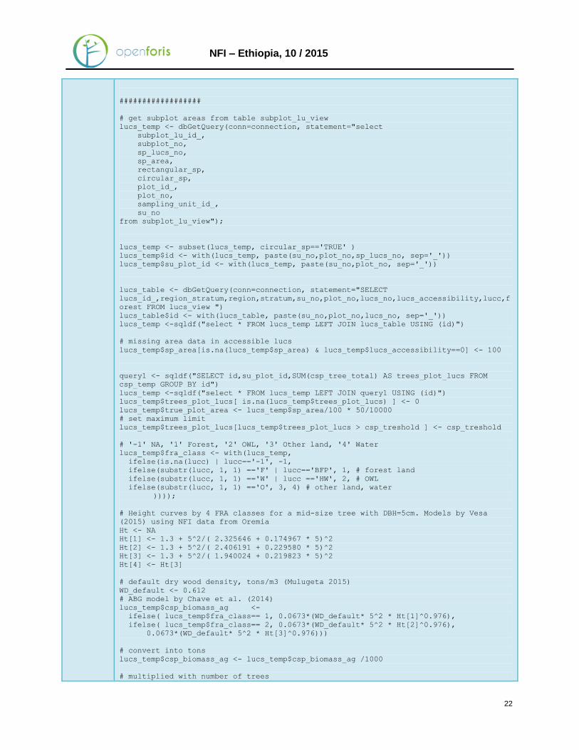
NFI – Ethiopia, 10 / 2015
##################
# get subplot areas from table subplot_lu_view
lucs_temp <- dbGetQuery(conn=connection, statement="select
subplot_lu_id_,
subplot_no,
sp_lucs_no,
sp_area,
rectangular_sp,
circular_sp,
plot_id_,
plot_no,
sampling_unit_id_,
su_no
from subplot_lu_view");
lucs_temp <- subset(lucs_temp, circular_sp=='TRUE' )
lucs_temp$id <- with(lucs_temp, paste(su_no,plot_no,sp_lucs_no, sep='_'))
lucs_temp$su_plot_id <- with(lucs_temp, paste(su_no,plot_no, sep='_'))
lucs_table <- dbGetQuery(conn=connection, statement="SELECT
lucs_id_,region_stratum,region,stratum,su_no,plot_no,lucs_no,lucs_accessibility,lucc,f
orest FROM lucs_view ")
lucs_table$id <- with(lucs_table, paste(su_no,plot_no,lucs_no, sep='_'))
lucs_temp <-sqldf("select * FROM lucs_temp LEFT JOIN lucs_table USING (id)")
# missing area data in accessible lucs
lucs_temp$sp_area[is.na(lucs_temp$sp_area) & lucs_temp$lucs_accessibility==0] <- 100
query1 <- sqldf("SELECT id,su_plot_id,SUM(csp_tree_total) AS trees_plot_lucs FROM
csp_temp GROUP BY id")
lucs_temp <-sqldf("select * FROM lucs_temp LEFT JOIN query1 USING (id)")
lucs_temp$trees_plot_lucs[ is.na(lucs_temp$trees_plot_lucs) ] <- 0
lucs_temp$true_plot_area <- lucs_temp$sp_area/100 * 50/10000
# set maximum limit
lucs_temp$trees_plot_lucs[lucs_temp$trees_plot_lucs > csp_treshold ] <- csp_treshold
# '-1' NA, '1' Forest, '2' OWL, '3' Other land, '4' Water
lucs_temp$fra_class <- with(lucs_temp,
ifelse(is.na(lucc) | lucc=='-1', -1,
ifelse(substr(lucc, 1, 1) =='F' | lucc=='BFP', 1, # forest land
ifelse(substr(lucc, 1, 1) =='W' | lucc =='HW', 2, # OWL
ifelse(substr(lucc, 1, 1) =='O', 3, 4) # other land, water
))));
# Height curves by 4 FRA classes for a mid-size tree with DBH=5cm. Models by Vesa
(2015) using NFI data from Oremia
Ht <- NA
Ht[1] <- 1.3 + 5^2/( 2.325646 + 0.174967 * 5)^2
Ht[2] <- 1.3 + 5^2/( 2.406191 + 0.229580 * 5)^2
Ht[3] <- 1.3 + 5^2/( 1.940024 + 0.219823 * 5)^2
Ht[4] <- Ht[3]
# default dry wood density, tons/m3 (Mulugeta 2015)
WD_default <- 0.612
# ABG model by Chave et al. (2014)
lucs_temp$csp_biomass_ag <-
ifelse( lucs_temp$fra_class== 1, 0.0673*(WD_default* 5^2 * Ht[1]^0.976),
ifelse( lucs_temp$fra_class== 2, 0.0673*(WD_default* 5^2 * Ht[2]^0.976),
0.0673*(WD_default* 5^2 * Ht[3]^0.976)))
# convert into tons
lucs_temp$csp_biomass_ag <- lucs_temp$csp_biomass_ag /1000
# multiplied with number of trees
23
NFI – Ethiopia, 10 / 2015
lucs_temp$csp_biomass_ag <- lucs_temp$csp_biomass_ag * lucs_temp$trees_plot_lucs
# default RS as 0.27 for small trees
lucs_temp$csp_biomass_bg <- 0.27 * lucs_temp$csp_biomass_ag
lucs_temp$csp_biomass_total <- lucs_temp$csp_biomass_ag + lucs_temp$csp_biomass_bg
lucs_temp$csp_carbon_ag <- 0.50 * lucs_temp$csp_biomass_ag
lucs_temp$csp_carbon_bg <- 0.50 * lucs_temp$csp_biomass_bg
lucs_temp$csp_carbon_total <- 0.50 * lucs_temp$csp_biomass_total
#write.csv(csp_temp, "c:/temp/csp_tree_summary.csv")
#write.csv(lucs_temp, paste(ResultFolder,"csp_lucs_summary.csv",sep=""))
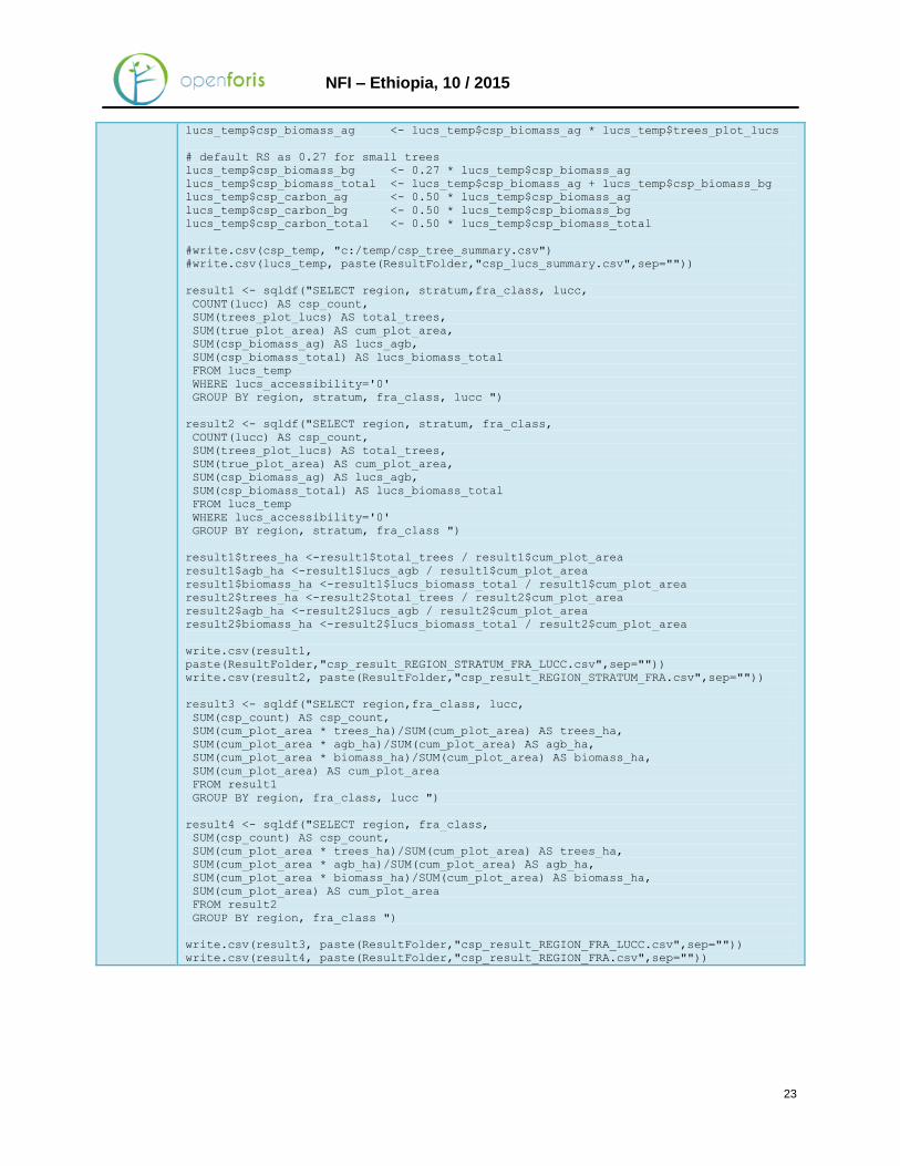
result1 <- sqldf("SELECT region, stratum,fra_class, lucc,
COUNT(lucc) AS csp_count,
SUM(trees_plot_lucs) AS total_trees,
SUM(true_plot_area) AS cum_plot_area,
SUM(csp_biomass_ag) AS lucs_agb,
SUM(csp_biomass_total) AS lucs_biomass_total
FROM lucs_temp
WHERE lucs_accessibility='0'
GROUP BY region, stratum, fra_class, lucc ")
result2 <- sqldf("SELECT region, stratum, fra_class,
COUNT(lucc) AS csp_count,
SUM(trees_plot_lucs) AS total_trees,
SUM(true_plot_area) AS cum_plot_area,
SUM(csp_biomass_ag) AS lucs_agb,
SUM(csp_biomass_total) AS lucs_biomass_total
FROM lucs_temp
WHERE lucs_accessibility='0'
GROUP BY region, stratum, fra_class ")
result1$trees_ha <-result1$total_trees / result1$cum_plot_area
result1$agb_ha <-result1$lucs_agb / result1$cum_plot_area
result1$biomass_ha <-result1$lucs_biomass_total / result1$cum_plot_area
result2$trees_ha <-result2$total_trees / result2$cum_plot_area
result2$agb_ha <-result2$lucs_agb / result2$cum_plot_area
result2$biomass_ha <-result2$lucs_biomass_total / result2$cum_plot_area
write.csv(result1,
paste(ResultFolder,"csp_result_REGION_STRATUM_FRA_LUCC.csv",sep=""))
write.csv(result2, paste(ResultFolder,"csp_result_REGION_STRATUM_FRA.csv",sep=""))
result3 <- sqldf("SELECT region,fra_class, lucc,
SUM(csp_count) AS csp_count,
SUM(cum_plot_area * trees_ha)/SUM(cum_plot_area) AS trees_ha,
SUM(cum_plot_area * agb_ha)/SUM(cum_plot_area) AS agb_ha,
SUM(cum_plot_area * biomass_ha)/SUM(cum_plot_area) AS biomass_ha,
SUM(cum_plot_area) AS cum_plot_area
FROM result1
GROUP BY region, fra_class, lucc ")
result4 <- sqldf("SELECT region, fra_class,
SUM(csp_count) AS csp_count,
SUM(cum_plot_area * trees_ha)/SUM(cum_plot_area) AS trees_ha,
SUM(cum_plot_area * agb_ha)/SUM(cum_plot_area) AS agb_ha,
SUM(cum_plot_area * biomass_ha)/SUM(cum_plot_area) AS biomass_ha,
SUM(cum_plot_area) AS cum_plot_area
FROM result2
GROUP BY region, fra_class ")
write.csv(result3, paste(ResultFolder,"csp_result_REGION_FRA_LUCC.csv",sep=""))
write.csv(result4, paste(ResultFolder,"csp_result_REGION_FRA.csv",sep=""))
24
NFI – Ethiopia, 10 / 2015
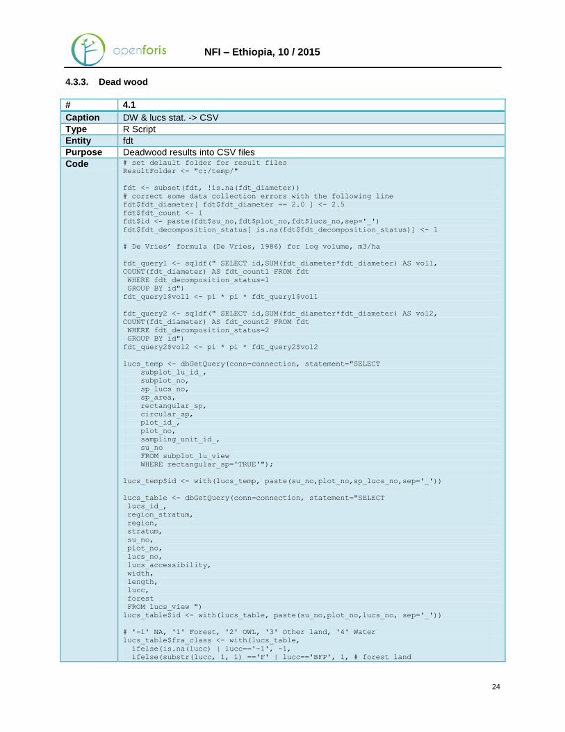
4.3.3. Dead wood
# 4.1
Caption DW & lucs stat. -> CSV
Type R Script
Entity fdt
Purpose Deadwood results into CSV files
Code # set delault folder for result files
ResultFolder <- "c:/temp/"
fdt <- subset(fdt, !is.na(fdt_diameter))
# correct some data collection errors with the following line
fdt$fdt_diameter[ fdt$fdt_diameter == 2.0 ] <- 2.5
fdt$fdt_count <- 1
fdt$id <- paste(fdt$su_no,fdt$plot_no,fdt$lucs_no,sep='_')
fdt$fdt_decomposition_status[ is.na(fdt$fdt_decomposition_status)] <- 1
# De Vries’ formula (De Vries, 1986) for log volume, m3/ha
fdt_query1 <- sqldf(" SELECT id,SUM(fdt_diameter*fdt_diameter) AS vol1,
COUNT(fdt_diameter) AS fdt_count1 FROM fdt
WHERE fdt_decomposition_status=1
GROUP BY id")
fdt_query1$vol1 <- pi * pi * fdt_query1$vol1
fdt_query2 <- sqldf(" SELECT id,SUM(fdt_diameter*fdt_diameter) AS vol2,
COUNT(fdt_diameter) AS fdt_count2 FROM fdt
WHERE fdt_decomposition_status=2
GROUP BY id")
fdt_query2$vol2 <- pi * pi * fdt_query2$vol2
lucs_temp <- dbGetQuery(conn=connection, statement="SELECT
subplot_lu_id_,
subplot_no,
sp_lucs_no,
sp_area,
rectangular_sp,
circular_sp,
plot_id_,
plot_no,
sampling_unit_id_,
su_no
FROM subplot_lu_view
WHERE rectangular_sp='TRUE'");
lucs_temp$id <- with(lucs_temp, paste(su_no,plot_no,sp_lucs_no,sep='_'))
lucs_table <- dbGetQuery(conn=connection, statement="SELECT
lucs_id_,
region_stratum,
region,
stratum,
su_no,
plot_no,
lucs_no,
lucs_accessibility,
width,
length,
lucc,
forest
FROM lucs_view ")
lucs_table$id <- with(lucs_table, paste(su_no,plot_no,lucs_no, sep='_'))
# '-1' NA, '1' Forest, '2' OWL, '3' Other land, '4' Water
lucs_table$fra_class <- with(lucs_table,
ifelse(is.na(lucc) | lucc=='-1', -1,
ifelse(substr(lucc, 1, 1) =='F' | lucc=='BFP', 1, # forest land
25
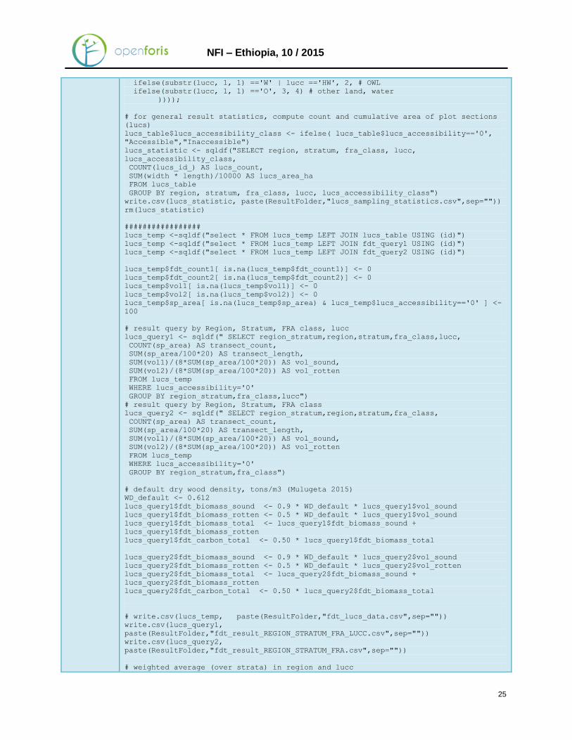
NFI – Ethiopia, 10 / 2015
ifelse(substr(lucc, 1, 1) =='W' | lucc =='HW', 2, # OWL
ifelse(substr(lucc, 1, 1) =='O', 3, 4) # other land, water
))));
# for general result statistics, compute count and cumulative area of plot sections
(lucs)
lucs_table$lucs_accessibility_class <- ifelse( lucs_table$lucs_accessibility=='0',
"Accessible","Inaccessible")
lucs_statistic <- sqldf("SELECT region, stratum, fra_class, lucc,
lucs_accessibility_class,
COUNT(lucs_id_) AS lucs_count,
SUM(width * length)/10000 AS lucs_area_ha
FROM lucs_table
GROUP BY region, stratum, fra_class, lucc, lucs_accessibility_class")
write.csv(lucs_statistic, paste(ResultFolder,"lucs_sampling_statistics.csv",sep=""))
rm(lucs_statistic)
#################
lucs_temp <-sqldf("select * FROM lucs_temp LEFT JOIN lucs_table USING (id)")
lucs_temp <-sqldf("select * FROM lucs_temp LEFT JOIN fdt_query1 USING (id)")
lucs_temp <-sqldf("select * FROM lucs_temp LEFT JOIN fdt_query2 USING (id)")
lucs_temp$fdt_count1[ is.na(lucs_temp$fdt_count1)] <- 0
lucs_temp$fdt_count2[ is.na(lucs_temp$fdt_count2)] <- 0
lucs_temp$vol1[ is.na(lucs_temp$vol1)] <- 0
lucs_temp$vol2[ is.na(lucs_temp$vol2)] <- 0
lucs_temp$sp_area[ is.na(lucs_temp$sp_area) & lucs_temp$lucs_accessibility=='0' ] <-
100
# result query by Region, Stratum, FRA class, lucc
lucs_query1 <- sqldf(" SELECT region_stratum,region,stratum,fra_class,lucc,
COUNT(sp_area) AS transect_count,
SUM(sp_area/100*20) AS transect_length,
SUM(vol1)/(8*SUM(sp_area/100*20)) AS vol_sound,
SUM(vol2)/(8*SUM(sp_area/100*20)) AS vol_rotten
FROM lucs_temp
WHERE lucs_accessibility='0'
GROUP BY region_stratum,fra_class,lucc")
# result query by Region, Stratum, FRA class
lucs_query2 <- sqldf(" SELECT region_stratum,region,stratum,fra_class,
COUNT(sp_area) AS transect_count,
SUM(sp_area/100*20) AS transect_length,
SUM(vol1)/(8*SUM(sp_area/100*20)) AS vol_sound,
SUM(vol2)/(8*SUM(sp_area/100*20)) AS vol_rotten
FROM lucs_temp
WHERE lucs_accessibility='0'
GROUP BY region_stratum,fra_class")
# default dry wood density, tons/m3 (Mulugeta 2015)
WD_default <- 0.612
lucs_query1$fdt_biomass_sound <- 0.9 * WD_default * lucs_query1$vol_sound
lucs_query1$fdt_biomass_rotten <- 0.5 * WD_default * lucs_query1$vol_sound
lucs_query1$fdt_biomass_total <- lucs_query1$fdt_biomass_sound +
lucs_query1$fdt_biomass_rotten
lucs_query1$fdt_carbon_total <- 0.50 * lucs_query1$fdt_biomass_total
lucs_query2$fdt_biomass_sound <- 0.9 * WD_default * lucs_query2$vol_sound
lucs_query2$fdt_biomass_rotten <- 0.5 * WD_default * lucs_query2$vol_rotten
lucs_query2$fdt_biomass_total <- lucs_query2$fdt_biomass_sound +
lucs_query2$fdt_biomass_rotten
lucs_query2$fdt_carbon_total <- 0.50 * lucs_query2$fdt_biomass_total
# write.csv(lucs_temp, paste(ResultFolder,"fdt_lucs_data.csv",sep=""))
write.csv(lucs_query1,
paste(ResultFolder,"fdt_result_REGION_STRATUM_FRA_LUCC.csv",sep=""))
write.csv(lucs_query2,
paste(ResultFolder,"fdt_result_REGION_STRATUM_FRA.csv",sep=""))
# weighted average (over strata) in region and lucc
26
NFI – Ethiopia, 10 / 2015
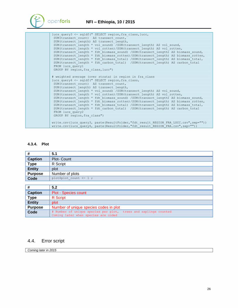
lucs_query3 <- sqldf(" SELECT region,fra_class,lucc,
SUM(transect_count) AS transect_count,
SUM(transect_length) AS transect_length,
SUM(transect_length * vol_sound) /SUM(transect_length) AS vol_sound,
SUM(transect_length * vol_rotten)/SUM(transect_length) AS vol_rotten,
SUM(transect_length * fdt_biomass_sound) /SUM(transect_length) AS biomass_sound,
SUM(transect_length * fdt_biomass_rotten)/SUM(transect_length) AS biomass_rotten,
SUM(transect_length * fdt_biomass_total) /SUM(transect_length) AS biomass_total,
SUM(transect_length * fdt_carbon_total) /SUM(transect_length) AS carbon_total
FROM lucs_query1
GROUP BY region,fra_class,lucc")
# weighted average (over strata) in region in fra_class
lucs_query4 <- sqldf(" SELECT region,fra_class,
SUM(transect_count) AS transect_count,
SUM(transect_length) AS transect_length,
SUM(transect_length * vol_sound) /SUM(transect_length) AS vol_sound,
SUM(transect_length * vol_rotten)/SUM(transect_length) AS vol_rotten,
SUM(transect_length * fdt_biomass_sound) /SUM(transect_length) AS biomass_sound,
SUM(transect_length * fdt_biomass_rotten)/SUM(transect_length) AS biomass_rotten,
SUM(transect_length * fdt_biomass_total) /SUM(transect_length) AS biomass_total,
SUM(transect_length * fdt_carbon_total) /SUM(transect_length) AS carbon_total
FROM lucs_query2
GROUP BY region,fra_class")
write.csv(lucs_query3, paste(ResultFolder,"fdt_result_REGION_FRA_LUCC.csv",sep=""))
write.csv(lucs_query4, paste(ResultFolder,"fdt_result_REGION_FRA.csv",sep=""))
4.3.4. Plot
# 5.1
Caption Plot- Count
Type R Script
Entity plot
Purpose Number of plots
Code plot$plot_count <- 1 ;
# 5.2
Caption Plot - Species count
Type R Script
Entity plot
Purpose Number of unique species codes in plot
Code # Number of unique species per plot, trees and saplings counted
Coming later when species are coded
4.4. Error script
Coming later in 2015

27
NFI – Ethiopia, 10 / 2015
References Chave, Jerome; Rejou-Mechain, Maxime; Burquez, Alberto; Chidumayo, Emmanuel; Colgan, Matthew S.; Delitti, Welington B. C.; Duque, Alvaro; Eid, Tron; Fearnside, Philip M.; Goodman, Rosa C.; Henry, Matieu; Martinez-Yrizar, Angelina; Mugasha, Wilson A.; Muller-Landau, Helene C.; Mencuccini, Maurizio; Nelson, Bruce W.; Ngomanda, Alfred; Nogueira, Euler M.; Ortiz-Malavassi, Edgar; Pelissier, Raphael; Ploton, Pierre; Ryan, Casey M.; Saldarriaga, Juan G.; Vieilledent, Ghislain. (2014). Improved allometric models to estimate the aboveground biomass of tropical trees. Global Change Biology, Vol. 20, No. 10, 26.06.2014, p. 3177-3190. [Applied in Calc: AGB model for trees] De Vries P.G., 1986. Sampling theory for forest inventory. A teach-yourself course, Springer-Verlag, Berlin, 420 p. [Applied in Calc: Equation to compute volume of deadwood in transect sampling] Mamo, Negaash; Habte, Berhane; Beyan, Dawit. (1995). Growth and form factor of some indigenous and exotic tree species in Ethiopia. Forestry Research Centre (Ethiopia). Forestry Research Centre, Ministry of Natural Resources Development and Environmental Protection. [To be applied in Calc: Form factors for bole volume of trees] Mehtätalo, Lauri; de-Miguel, Sergio; Gregoire, Timothy G. (2015). Modeling height-diameter curves for prediction. Can. J. For. Res. 45: 826–837. [Applied in Calc: Height curve for trees]