Any correspondence concerning this service should be sent to the repository administrator:

staff-oatao@inp-toulouse.fr

Identification number: DOI: 10.1063/1.4866043

Official URL: http://dx.doi.org/10.1063/1.4866043

This is an author-deposited version published in: http://oatao.univ-toulouse.fr/

Eprints ID: 11796

To cite this version:

Del Guercio, Gerardo and Cossu, Carlo and Pujals, Grégory Optimal

perturbations of non-parallel wakes and their stabilizing effect on the global

instability. (2014) Physics of Fluids, vol. 26 (n° 2). 024110-1-024110-14. ISSN

1070-6631

Open Archive Toulouse Archive Ouverte (OATAO) OATAO is an open access repository that collects the work of Toulouse researchers and

makes it freely available over the web where possible.

Optimal perturbations of non-parallel wakes and theirstabilizing effect on the global instability

Gerardo Del Guercio,1,2 Carlo Cossu,1 and Gregory Pujals2

1Institut de Mecanique des Fluides de Toulouse, CNRS and Universite de Toulouse,Allee du Professeur Camille Soula, 31400 Toulouse, France2PSA Peugeot Citroen, Centre Technique de Velizy, 2 Route de Gisy,78943 Velizy-Villacoublay Cedex, France

We compute the spatial optimal energy amplification of steady inflow perturbations ina non-parallel wake and analyse their stabilizing action on the global mode instability.The optimal inflow perturbations, which are assumed spanwise periodic and varicose,consist in streamwise vortices that induce the downstream spatial transient growth ofstreamwise streaks. The maximum energy amplification of the streaks increases withthe spanwise wavelength of the perturbations, in accordance with previous resultsobtained for the temporal energy growth supported by parallel wakes. A family ofincreasingly streaky wakes is obtained by forcing optimal inflow perturbations ofincreasing amplitude and then solving the nonlinear Navier-Stokes equations. Weshow that the linear global instability of the wake can be completely suppressed byforcing optimal perturbations of sufficiently large amplitude. The attenuation andsuppression of self-sustained oscillations in the wake by optimal 3D perturbations isconfirmed by fully nonlinear numerical simulations. We also show that the amplitudeof optimal spanwise periodic (3D) perturbations of the basic flow required to stabilizethe global instability is much smaller than the one required by spanwise uniform (2D)perturbations despite the fact that the first order sensitivity of the global eigenvalue tobasic flow modifications is zero for 3D spanwise periodic modifications and non-zerofor 2D modifications. We therefore conclude that first-order sensitivity analyses can bemisleading if used far from the instability threshold, where higher order terms are themost relevant.

I. INTRODUCTION

Two-dimensional wakes behind bluff bodies support robust self-sustained vortex shedding forsufficiently large Reynolds numbers. The onset of self-sustained oscillations is associated to a globalinstability supported by a finite region of local absolute instability in the near wake.1–3 There is acontinued interest in controlling vortex shedding because, in addition to inducing unsteady loads onthe body, it also leads to an increase of the mean drag.

Spanwise periodic (3D) perturbations of spanwise uniform (2D) wakes, e.g., obtained withperiodic modulations of the trailing and/or leading edge of the bluff body4–7 or spanwise periodicblowing and suction8 can attenuate and even suppress vortex shedding and reduce the associatedundesired drag and unsteady loads (see, e.g., Ref. 9 for a review). Recently, important progress hasbeen made in the understanding of this stabilizing action from a linear stability perspective: Hwanget al.10 show that appropriate 3D spanwise periodic perturbations of 2D absolutely unstable wakeprofiles lead to a reduction of the absolute growth rate. This reduction is observed for a range ofspanwise wavelengths that is in accordance with experimental results, just as the fact that varicoseperturbations are more stabilizing than sinuous ones. However, the question of the higher efficiencyof 3D perturbations when compared to 2D ones in reducing the absolute growth rate was left partiallyopen by this study. It is indeed known that lower rates of 3D blowing and suction, compared to 2Done, are required to suppress shedding in a cylinder wake.8 This seems to contrast the fact that the

This article is copyrighted as indicated in the article. Reuse of AIP content is subject to the terms at: http://scitation.aip.org/termsconditions. Downloaded to IP:

195.83.231.74 On: Mon, 24 Feb 2014 17:07:04

first-order sensitivity of the absolute instability growth rate with respect to 3D spanwise periodicmodifications of the basic flow is zero,10, 11 therefore predicting that, at first order, 2D perturbationsare more effective than 3D ones in reducing the absolute growth rate.

A partial explanation of the higher efficiency of 3D perturbations when compared to 2D oneshas been given in another recent study12 where we show that parallel “frozen” 2D wakes cansupport the large temporal amplification of streamwise streaks from stable spanwise periodic andstreamwise uniform streamwise vortices via the lift-up effect.13, 14 The optimal perturbations leadingto the optimal amplification of the streaks were computed and it was shown that varicose streaks ofrelatively small amplitude are able to completely quench the absolute instability.12 It was also shownthat the initial amplitude of optimal 3D perturbations necessary to quench the absolute instability ismuch smaller than the initial amplitude required by 2D perturbations.

Many questions were however left unanswered by the local temporal analysis developed inour previous investigation.12 For instance, can optimal spatial amplifications be large in spatiallydiffusing wakes? The answer is not a priori clear because the wake diffusion not only reduces thebasic flow shear fuelling the transient growth but also increases the local spanwise wavenumberof the perturbation, which is known from local analysis to reduce the growth. Another question is:are 3D optimal perturbations more efficient than 2D ones in stabilizing a global instability? Theanswer to this question is not obvious because finite downstream distances are needed to attain themaximum energy growth, while the pocket of absolute instability that needs to be controlled is lo-cated upstream, and therefore it is not clear how efficient optimal perturbations can be in quenchingthe absolute instability. The scope of the present study is to answer these questions by consid-ering the spatial optimal perturbations and their influence on the global stability of non-parallelwakes.

An “artificial” wake, left free to spatially develop downstream the enforced inflow wake profile,is introduced as reference 2D basic flow in Sec. III. The use of such a basic flow allows us tofind results which are independent of the specific body shape generating the wake and of theparticular devices used to generate the optimal perturbations. The optimal spatial perturbationsof this non-parallel wake are computed in Sec. IV following the procedure described in Sec. II.These optimal perturbations are defined as the perturbation profiles enforced at the inflow stationthat lead to the optimal energy amplification G(x) at the downstream station x. This definition isquite different from that of optimal initial or inflow conditions leading to the optimal temporalenergy amplification15, 16 G(t). Optimal spatial energy amplifications have already been computedin non-parallel boundary layers by using direct-adjoint methods exploiting the parabolic nature ofthe boundary layer equations.17, 18 Here we choose to specifically design an alternative scalableoptimization method (see Sec. II) that does not rely on the parabolic nature of the equations andthat does not require the explicit computation of adjoint operators. The influence of forcing optimalperturbations on the global linear stability is investigated in Sec. V. The results of fully nonlinearsimulations that validate these results in the nonlinear regime are reported in Sec. V D, while theused numerical methods are summarized in the Appendix.

II. PROBLEM FORMULATION

In this section the mathematical formulation of the analysis performed in the paper is brieflyintroduced. The formulation is general and can be applied to other non-parallel shear flows. Specificdetails about the particular wake profile and perturbations used in this study are mentioned inSecs. III–V.

A reference two-dimensional (2D) non-parallel plane basic flow U2D(x, y) is obtained as a steadysolution of the Navier-Stokes equations with inflow boundary condition U = U0(y)ex given at x = 0and free-stream conditions U → U∞ex given as y → ±∞. We denote by x, y, and z the streamwise,cross-stream, and spanwise coordinates and by ex , ey , ez the associated unit vectors. The Reynoldsnumber Re = U ∗

re f δ∗/ν is based on the characteristic velocity and length associated to U0(y) and on

the kinematic viscosity ν of the fluid. The non-parallel basic flow U2D = U (x, y)ex + V (x, y)ey isinvariant to translations and reflections in the spanwise coordinate z (it is therefore two-dimensionalor 2D).

This article is copyrighted as indicated in the article. Reuse of AIP content is subject to the terms at: http://scitation.aip.org/termsconditions. Downloaded to IP:

195.83.231.74 On: Mon, 24 Feb 2014 17:07:04

Perturbations u′ to the reference 2D basic flow are ruled by the Navier-Stokes equations inperturbation form:

∇ · u′ = 0, (1)

∂u′

∂t+ (∇U) u′ + (∇u′) U + (∇u′) u′ = −∇ p′ + 1

Re∇2u′, (2)

using U = U2D as basic flow.In the first part of the study, dealing with optimal spatial perturbations of U2D , we consider steady

perturbations u′ of U2D obtained by perturbing the inlet profile U0(y) with steady inflow perturbationsu′

0(y, z). We are interested in steady perturbations both because they are spatially stable and becausethey are of interest in passive control applications. In particular, spanwise periodic perturbations ofwavelength λz will be considered in the following. Considering small perturbations, the nonlinearterm (∇u′)u′ can be neglected, which makes the perturbation equations linear. Defining the localperturbation kinetic energy density as

e′(x) = 1

2δλz

∫ ∞

−∞

∫ λz

0u′ · u′ dy dz, (3)

the optimal spatial energy amplification of inflow perturbations is defined as

G(x) = maxu′

0

e′(x)

e′0

. (4)

Different approaches can be used to compute G(x) and the associated optimal inflow perturbation.We choose here to decompose the inlet perturbation on a set of linearly independent functions b(m)

0 ,in practice limited to M terms, as

u′0(y, z) =

M∑m=1

qmb(m)0 (y, z). (5)

Denoting by b(m)(x, y, z) the perturbation velocity field obtained using b(m)0 (y, z) as inlet perturba-

tion, from the linearity of the operator follows that

u′(x, y, z) =M∑

m=1

qmb(m)(x, y, z), (6)

where the coefficients qm are the same used in Eq. (5). The optimization problem in Eq. (4) cantherefore be recast in terms of the M-dimensional control vector q as

G(x) = maxq

qT H(x)qqT H0q

, (7)

where the components of the symmetric matrices H(x) and H0 are

Hmn(x) = 1

2δλz

∫ ∞

−∞

∫ λz

0b(m)(x, y, z) · b(n)(x, y, z) dy dz, (8)

H0,mn = 1

2δλz

∫ ∞

−∞

∫ λz

0b(m)

0 (y, z) · b(n)0 (y, z) dy dz. (9)

Within this formulation G(x) is easily found as the largest eigenvalue μmax of the generalizedM × M eigenvalue problem μH0w = Hw. The corresponding eigenvector is the optimal set ofcoefficients q(opt) maximizing the kinetic energy amplification at the selected streamwise station x.The corresponding inlet perturbation is u′(opt)

0 (y, z) = ∑Mm=1 q (opt)

m b(m)0 (y, z). In the limit M → ∞

the approximated solution converges to the exact solution.In the second part of the study, the influence of forcing finite amplitude optimal perturbations

on linear global stability is investigated. A family of 3D streaky nonlinear non-parallel basic flows

This article is copyrighted as indicated in the article. Reuse of AIP content is subject to the terms at: http://scitation.aip.org/termsconditions. Downloaded to IP:

195.83.231.74 On: Mon, 24 Feb 2014 17:07:04

U3D(x, y, z; A0) is obtained by looking for steady solutions of the (nonlinear) Navier-Stokes equa-tions with inflow boundary condition U0(y, z) = U0(y)ex + A0u′(opt)

0 (y, z) given at x = 0. u′(opt)0 is

normalized to unit x-local energy so that e′(0) = A20 for u′ = U3D − U2D (see the definition of e′ in

Eq. (3)). In general, it is not guaranteed that the linear optimal perturbations are also (nonlinearly)optimal at finite amplitude. However, for the present purpose of open-loop control, this is not aproblem as long as they are still largely amplified. Using strictly optimal perturbations is also notcritical because it is not likely that strictly optimal perturbations can be forced in a real flow andthere is no guarantee that they would be also the optimal ones in reducing the global mode growthrate. The global linear stability of the U3D basic flows is then analysed by integrating in time thelinearized form of the Navier-Stokes equations (1) and (2) in perturbation form with U = U3D . Afterthe extinction of transients, the leading global mode emerges inducing an exponential growth ordecay of the solution. The global growth rate is then deduced from the slope of the global energyamplification curve.

III. NON PARALLEL 2D REFERENCE WAKE

The 2D reference wake is computed by enforcing as inflow boundary condition the followingwell studied2 wake profile:

U0(y) = 1 + �

[2

1 + sinh2N (y sinh−1 1)− 1

], (10)

with � = (U ∗c − U ∗

∞)/(U ∗∞ + U ∗

c ), where U ∗c is the centreline and U∞∗ the freestream velocity (di-

mensional variables are starred). The velocity U0 is made dimensionless with respect to the referencevelocity U ∗

re f = (U ∗c + U ∗

∞)/2. The spatial coordinates are made dimensionless with respect to thereference length δ∗

0 that is the distance from the centreline to the point where the 2D wake velocityis equal to U ∗

re f , computed at the inflow. We set � = −1.35 to ensure a small recirculation in theupstream region of the wake. For � = −1.35, the wake is globally unstable when Re � 39 (notshown). In the following we will consider the value Re = 50 for which numerical simulation (seethe Appendix for the numerical details) shows strong self-sustained oscillations in the wake (seeFig. 1(b)). As at Re = 50 the only unstable global mode is sinuous (antisymmetric with respect tothe y = 0 axis), the unstable basic flow U2D is computed by direct temporal integration by enforcingthe y-symmetry of the solutions (otherwise a Newton-based continuation method would have beenrequired). The reference basic flow is shown in Fig. 1(a). It can be seen how the basic flow vorticity,which is maximum at x = 0 with peaks at y ≈ ±1, slowly diffuses downstream.

(a)

(b)

x

y

0 10 20 30 40 50 60−10

−10

−5

−5

0

5

10

x

y

0 10 20 30 40 50 60

0

5

10

FIG. 1. Spanwise vorticity fields ωz(x, y) associated to the reference 2D non-parallel wake at Re = 50. (a) (unstable) Basic 2Dflow profile obtained by enforcing the y-symmetry of the solution. (b) Snapshot of the periodic self-sustained state obtainedwithout enforcing the y-symmetry of the solution.

This article is copyrighted as indicated in the article. Reuse of AIP content is subject to the terms at: http://scitation.aip.org/termsconditions. Downloaded to IP:

195.83.231.74 On: Mon, 24 Feb 2014 17:07:04

0

10

20

30

20 40 60 80 100 120

x

G

(a)

β

0

10

20

30

0.25 0.75 1.25 1.75

β

Gmax

(b)

FIG. 2. Optimal spatial energy growths G(x) (panel (a)) computed for the spanwise wavenumbers β = 0.5, 0.75, . . . , 1.50,1.75 at Re = 50 (outer to inner). The dependence Gmax(β) of the maximum energy growths on the spanwise wavenumber isreported in panel (b).

IV. OPTIMAL SPATIAL ENERGY GROWTH

Optimal steady inlet perturbations of U2D maximizing the spatial energy amplification G(x) arecomputed following the procedure described in Sec. II. Our previous investigation of the optimaltemporal energy growth in parallel wakes12 has shown that the most amplified spanwise periodicand streamwise uniform (corresponding to steady in our spatial framework) perturbations consistin streamwise vortices inducing the growth of streamwise streaks. We therefore consider inlet con-ditions of the type: u′

0 = (u′0, v

′0, w

′0) = (0, ∂ψ/∂z,−∂ψ/∂y). Single-harmonic spanwise periodic

perturbations can be considered without loss of generality: ψ ′ = f(y)sin (βz). As varicose pertur-bations (mirror-symmetric with respect to the y = 0 plane) are the most efficient for control,9, 10, 12

even if they are slightly less amplified than sinuous ones,12 we enforce f (−y) = −f(y) which leadsto varicose streaks. The set of linearly independent inflow conditions used in Eq. (5) is chosen asb(m)

0 (y, z) = (0, ∂ψ (m)/∂z,−∂ψ (m)/∂y) with ψ (m) = fm(y)sin (βz) and fm(y) = −fm(y) for m = 1,. . . , M. We have found well suited the set fm(y) = sin (2mπy/Ly), where the numerical box extendsfrom −Ly/2 to Ly/2 in the y direction.

Optimal energy growths have been computed for a set of spanwise wavenumbers β increasingM until a precision of 1% or higher on Gmax was achieved (see also the Appendix for the numericaldetails of the computations). The computed optimal energy growth curves G(x, β) are reportedin Fig. 2(a). It is seen how, consistently with results form the local analysis,12 both the maximumgrowth Gmax = max xG(x) and the position xmax where it is attained increase with increasing spanwisewavelength λz = 2π /β, i.e. with decreasing β (see also panel (b) of the same figure). The convergenceof the optimal growth curves with increasing M is quite fast, and this for all the considered values ofβ, as can be seen in Fig. 3. Well converged results, with relative variations below 1% are obtainedwith only M = 16 terms.

0

5

10

15

20

25

20 40 60 80 100 120

x

G

(a)M=16M=12

M=8M=4M=2

0

10

20

30

0.25 0.75 1.25 1.75

β

Gmax

(b)M=16M=12

M=8M=4M=2

FIG. 3. Convergence of the optimal energy growth G(x) for β = 1 (panel (a)) and of the maximum energy growth Gmax(β)(panel (b)) when the number M of linearly independent inflow conditions is increased at Re = 50. Well converged results areobtained for M = 16.

This article is copyrighted as indicated in the article. Reuse of AIP content is subject to the terms at: http://scitation.aip.org/termsconditions. Downloaded to IP:

195.83.231.74 On: Mon, 24 Feb 2014 17:07:04

z

y

−3 −2 −1 0 1 2 3

−3

−2

−1

0

1

2

3

FIG. 4. Cross-stream (y-z) view of the cross-stream v′0-w′

0 components of optimal vortices (arrows) forced at the inflow(x = 0) and of the streamwise u′ component of the corresponding optimal streaks (contour-lines) at x = xmax for Re = 50,β = 1. The 2D basic flow wake streamwise velocity at the inflow U0(y) is also reported in grey-scale with white correspondingto the freestream velocity and dark grey the minimum velocity (wake centreline).

The optimal inflow perturbations (x = 0) and the maximum response (x = xmax) associated tothe maximum growth Gmax obtained for β = 1 are reported in Fig. 4. The corresponding velocityprofiles are reported in Fig. 5, where additional values of β are also considered. The optimal inflowperturbations consist in two rows of counter-rotating vortices on each side of the y = 0 plane, withopposite rotation on each side. These vortices induce the growth of y-symmetric (varicose) streaks.From Fig. 5 it can be seen how, for increasing spanwise wavelengths λz (decreasing β), the sizeof optimal perturbations increases in the normal (y) direction (and of course also in the spanwise zdirection).

The observed trends are in agreement with those found in our previous local analysis.12 However,the maximum spatial growth rates obtained in the non-parallel case are smaller than the temporalones obtained at the same nominal β under the frozen and parallel flow approximation. This isnot surprising because the nominal values of β and Re of the non-parallel results are based on theproperties of the wake profile at the inflow (x = 0). As the dimensional reference length δ∗(x) (the y∗

-10

-5

0

5

10

-1 0 1

vopt (x=0)

y(a)

-10

-5

0

5

10

-1 0 1

wopt (x=0)

y(b)

-10

-5

0

5

10

0 1

uopt (xmax)

y(c)

FIG. 5. Normalized amplitude of the v(x = 0, y, z = 0) component (panel (a)) and w(x = 0, y, z = λz/4) components(panel (b)) of the optimal inflow boundary vortices. The normalized amplitude of the u(x = xmax, y, z = 0) streamwisecomponent of the corresponding optimally amplified streaks is plotted in panel (c). Three selected spanwise wavenumbersare considered: β = 0.5 (dashed line, green), β = 1 (solid line, red), and β = 1.5 (dotted line, blue).

This article is copyrighted as indicated in the article. Reuse of AIP content is subject to the terms at: http://scitation.aip.org/termsconditions. Downloaded to IP:

195.83.231.74 On: Mon, 24 Feb 2014 17:07:04

value where U ∗2D(y∗) = U ∗

re f ) increases with x, a dimensionless wavenumber β = β∗δ∗ based on thelocal scale would increase going downstream. As the maximum growth rate is a decreasing functionof β, it is not surprising that the maximum growth rates are smaller than the ones that would beobtained if the wake was parallel. Therefore, the results of the present analysis should be comparedto the ones of the local analysis obtained at larger values of β.

V. STABILIZING EFFECT OF OPTIMALLY FORCED STREAKS ON GLOBAL MODES

In this second part of the study, we investigate the influence of the forcing of optimal per-turbations on the linear global stability of the wake. The input parameter of this analysis is theamplitude A0 of the forcing at the inflow boundary and the output is the linear growth rate sr

of the global mode supported by the streaky wake. All the results are obtained for Re = 50 andβ = 1. The choice of β = 1 is not completely arbitrary. On the one hand, in order to obtain largeenergy amplifications, one should choose low values of β. For low β, however, not only would thecross-stream size of the inlet optimal vortices be probably too large to be implemented in practicalapplications but, even more importantly, large amplitudes of the streaks would be obtained onlyfar downstream (e.g., xmax ≈ 120 for β = 0.5). This is a problem because the main scope of thecontrol is to reduce the absolute growth rate in the absolute region which extends up to x ≈ 5.On the other hand, selecting large values of β, in order to have xmax in the absolute region, wouldlead to poor energy amplifications and would exclude any damping in the convective region. Thevalue β = 1 is a good compromise between these two extrema. In particular, as can be seen fromFig. 2(a), the obtained G(x) for β = 1 in the region x � 10 are sensibly the same of those obtainedfor higher β.

A. Streaky wakes basic flows

Non-parallel streaky (3D) wake basic flows U3D(x, y, z; A0) are computed by enforcing atx = 0 the inflow condition U = U0(y)ex + A0u′(opt)

0 and by then computing the correspondingsteady solution of the (nonlinear) Navier-Stokes equations, as explained in Sec. II. The solution,which may be unstable, is obtained by enforcing symmetry with respect to the y = 0 plane, exactlyas done to compute U2D . The local amplitude of the streaks is measured extending the standarddefinition used in previous studies:12, 19

As(x) = 1

2

maxy,z

(U3D − U2D

)− miny,z

(U3D − U2D

)maxy U0 − miny U0

. (11)

In this definition the streak amplitude at the station x is defined as half the maximum deviation of thestreaky 3D profile from the reference 2D profile, at the same x station, normalized by the maximumvelocity variation of the inflow 2D reference profile.

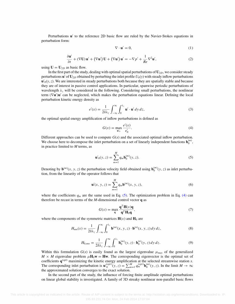
The considered values of A0 and the obtained values of As at xmax (maximum value of As) andin the middle of the absolute instability region (x = 2.7) are reported in Table I, where eachconsidered case is given a literal label. Case A corresponds to the reference two-dimensionalwake profile U2D (no streaks) while cases B, C, D, and E are obtained by increasing the inletamplitude A0 of the forced optimal perturbations. The nonlinear streaks amplitude evolution As(x)associated to the velocity fields U3D are reported in Fig. 6(a) for the considered cases. FromFig. 7, where streaky basic flows are shown in the symmetry plane y = 0, it is seen how, indeedfor increasing A0, the wake is increasingly 3D. The effect of nonlinearity is to slightly reduce themaximum energy growth (from ≈20 in the linear small amplitude limit to ≈17–15 for streaks D andE, not shown) and to induce a mean flow distortion that slightly counteracts the effect of the streaks.

B. Linear global stability analysis

The linear global stability analysis is performed via a direct numerical simulation of theNavier-Stokes equations (1) and (2) linearized upon the 3D streaky basic flows U3D defined above(Sec. V A). In previous local stability analyses10, 12 it was shown that for large streaks amplitudes,

This article is copyrighted as indicated in the article. Reuse of AIP content is subject to the terms at: http://scitation.aip.org/termsconditions. Downloaded to IP:

195.83.231.74 On: Mon, 24 Feb 2014 17:07:04

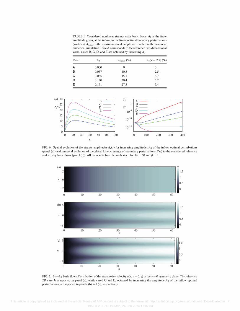
TABLE I. Considered nonlinear streaky wake basic flows. A0 is the finiteamplitude given, at the inflow, to the linear optimal boundary perturbations(vortices). As,max is the maximum streak amplitude reached in the nonlinearnumerical simulation. Case A corresponds to the reference two-dimensionalwake. Cases B, C, D, and E are obtained by increasing A0.

Case A0 As,max (%) As(x = 2.7) (%)

A 0.000 0 0B 0.057 10.3 2.5C 0.085 15.1 3.7D 0.120 20.4 5.2E 0.171 27.3 7.4

0

5

10

15

20

25

30

0 20 40 60 80 100 120

x

As%

(a)BCDE

10-15

10-10

10-5

1

0 100 200 300 400

t

E’

(b)ABCDE

FIG. 6. Spatial evolution of the streaks amplitudes As(x) for increasing amplitudes A0 of the inflow optimal perturbations(panel (a)) and temporal evolution of the global kinetic energy of secondary perturbations E′(t) to the considered referenceand streaky basic flows (panel (b)). All the results have been obtained for Re = 50 and β = 1.

(a)

(b

(c

)

x

z

0 10 20 30 40 50 60

−2

5

−5

−5

0

2

0

0.5

1

1.5

x

z

0 10 20 30 40 50 60

0

0

0.5

1

1.5

)

x

z

0 10 20 30 40 50 60

0

5

0

0.5

1

1.5

FIG. 7. Streaky basic flows. Distribution of the streamwise velocity u(x, y = 0, z) in the y = 0 symmetry plane. The reference2D case A is reported in panel (a), while cased C and E, obtained by increasing the amplitude A0 of the inflow optimalperturbations, are reported in panels (b) and (c), respectively.

This article is copyrighted as indicated in the article. Reuse of AIP content is subject to the terms at: http://scitation.aip.org/termsconditions. Downloaded to IP:

195.83.231.74 On: Mon, 24 Feb 2014 17:07:04

the dominant absolute mode is subharmonic, i.e., its spanwise wavelength is twice that of the basicflow streaks. This is taken in due consideration by integrating the linearized equations in a domainincluding two basic flow streaks wavelengths (Lz = 2λz). Noisy initial conditions on u′ are given forthe reference 2D wake (case A). The unstable global mode emerging for large times in the reference2D wake is then used, upon normalization of its amplitude, as initial condition on u′ in simulationswith the increasingly streaky basic flows B,...,E.

The temporal evolution of the global perturbation kinetic energy

E ′ = 1

2δLx Lz

∫ Lx

0

∫ L y/2

−L y/2

∫ Lz

0u′ · u′ dx dy dz

is reported in Fig. 6(b). After an initial transient extending to t ≈ 70, the dependence of E′ on timeis exponential (a straight line in the lin-log scales used in the figure), where the rate of growth or ofdecay is twice the growth rate of the global mode.

As anticipated (see, e.g., Fig. 1(b)) the reference 2D wake (case A) is strongly linearly unstableat Re = 50. The forcing of 3D linearly optimal perturbations of increasing amplitude has a stabilizingeffect on the global instability. The growth rate first reduced for low amplitude streaks (cases B andC) is then rendered quasi-neutral (case D) and finally completely stable for sufficiently large streakamplitudes (case E).

In the neutral and stable case the streaks amplitudes As(x = 2.7), measured in the middle ofthe absolute instability region of the reference 2D wake, are respectively of ≈5% and ≈7%. Thesevalues are not far from the ≈8% value at which the absolute instability was completely quenched inour previous local stability analysis.12 Also remark that, in the present non-parallel case As is givenin terms of the entrance reference maximum �U2D(x = 0), but if it was based on the local valueof �U2D(x) which is decreased with x, this would result in even larger downstream values of As.The stabilization of the global mode therefore appears to be associated to a strong reduction of thepocket of absolute instability that drives the global mode oscillations in the 2D reference case. Alocal stability analysis of the basic flow profiles extracted at x = 2.7 (not shown) indeed confirms thatthe local absolute growth rate is reduced with increasing streak amplitudes and that it is completelyquenched by streak E.

C. Sensitivity of the global growth rate to the amplitude of 3D optimal structures

1. The first order sensitivity of the global growth rate to streaks is zero

In previous studies based on local stability analyses,10, 11 it was shown that the sensitivity of theabsolute growth rate to 3D spanwise periodic modifications of the basic flow is zero. The argumentdeveloped in the local absolute instability analysis is easily extended to the global stability analysis ofthe nonparallel wake and proceeds as follows. Denote by L2D the Navier-Stokes operator linearizednear the 2D basic flow U2D . For small values of the inflow amplitude of optimal perturbations,the basic flow is modified by a small amount δU = U3D − U2D that induces a small change δLin the linear operator. At first order, the change of the leading eigenvalue induced by this smallvariation is20, 21 δs = 〈w†

2D, δLw2D〉/〈w†2D, w2D〉, where w2D, s2D, w†

2D are, respectively, the leadingglobal mode, eigenvalue, and adjoint global mode associated to U2D , and the standard inner productis defined as 〈a, b〉 = ∫ Lx

0

∫ L y/2−L y/2

∫ Lz

0 a · b dx dy dz. From Eq. (2) it is seen that the variation δLinduced by δU consists only in spanwise periodic terms as δU is itself spanwise periodic. As w2D

and w†2D do not depend on z, it follows22 that 〈w†, δLw〉 = 0 and therefore that δs = 0. This is not the

case for 2D (spanwise uniform) perturbations of U for which the variation of the leading eigenvalueis, in general, non-zero.

2. Effective sensitivity of global growth rate to spanwise periodic basic flowmodifications and comparison with 2D modifications

We now consider the observed dependence of the most unstable global mode on the controlamplitude. Such a control amplitude is unequivocally defined in terms of inflow optimal perturbation

This article is copyrighted as indicated in the article. Reuse of AIP content is subject to the terms at: http://scitation.aip.org/termsconditions. Downloaded to IP:

195.83.231.74 On: Mon, 24 Feb 2014 17:07:04

-4

-2

0

2

4

0 0.05 0.1 0.15 0.2

A0

s r*1

00

(a)

3D2D -4

-2

0

2

4

0 5 10 15 20 25 30

As%(x=2.7)

s r*1

00

(b)

3D2D 3

3.3

0 0.5 1 1.5

As%(x=2.7)

s r*1

00

(c)

3D2D

FIG. 8. Dependence of the growth rate of the global eigenvalue sr on the inflow optimal perturbation amplitude A0

(panel (a)) and on the streak amplitude As(x = 2.7) measured in the centre of the absolute region of the reference 2Dwake (panels (b) and (c) for a zoomed plot). A spanwise uniform perturbation (2D) has been also considered for comparison.Symbols denote data points, while lines are best fits to the data points.

amplitudes A0. The dependence of the global growth rate sr on the inflow optimal perturbationamplitude A0 is displayed in Fig. 8(a). If this dependence is also to be reported in term of streaksamplitudes, for the considered streaks with β = 1, it makes no sense to report it in terms of As,max

because this value is attained far downstream, in the convectively unstable region. We instead takeas an indicator of the “useful” streak amplitude the amplitude of the streaks in the middle of theabsolute region of the unperturbed flow As(x = 2.7). The dependence of sr on this amplitude isreported in Fig. 8 (panels (b) and (c) for a zoom).

In the same figures the variation of the growth rate sr induced by a 2D perturbation of the basicflow is also reported for comparison. The 2D perturbation has the same y shape as the optimal streakshape in the middle of the absolute region (x = 2.7) but is uniform instead of periodic in the spanwisedirection. For this 2D perturbation, A0 is unambiguously defined and As is defined as the maximumassociated �U taken at x = 2.7.

From the figures it is clearly seen how the first order sensitivities dsr/dA0 and dsr/dAs computedfor A0 = As = 0 are zero for the 3D perturbations and non-zero for the 2D perturbations as predictedby the first order sensitivity analysis. According to a first-order sensitivity analysis one would expectthe 2D perturbations to be more effective than 3D ones in quenching the global instability, but exactlythe opposite is observed. Indeed, 2D perturbations are more effective than 3D ones in reducing sr

only for very small perturbation amplitudes, while the opposite is observed for larger amplitudeswhere the higher order dependence of sr on A0 and As induces more important reductions of sr. Weindeed find that 3D perturbations stabilize the global mode at a value of As(x = 2.7) more than fivetimes smaller, and more than ten times smaller in terms of A0. A higher efficiency of 3D perturbationswas expected for results expressed in terms of A0, due to the gain associated with the lift-up of the3D optimal perturbations. However, such a result was somehow unexpected when expressing thegrowth rate reductions in terms of As.

D. Nonlinear simulations

Non-linear simulations of the full Navier-Stokes equations have finally been performed to assessthe effect of the inflow forcing of 3D optimal perturbations in the nonlinear regime. The same gridused in linear simulations has been used in the nonlinear ones. In a first simulation, the permanentharmonic self-sustained state supported by the reference 2D wake is allowed to develop. This 2D(spanwise uniform) self-sustained state is then given as an initial condition to simulations in thepresence of the optimal perturbations (streaky wakes) of increasing amplitude. As expected from thelinear analysis, the global perturbation kinetic energy E′ associated to the self-sustained oscillationsin the wake is reduced when the amplitude of the enforced optimal perturbations is increased (seeFig. 9). A stable steady streaky wake is found for case E, where the oscillations are completelysuppressed.

This article is copyrighted as indicated in the article. Reuse of AIP content is subject to the terms at: http://scitation.aip.org/termsconditions. Downloaded to IP:

195.83.231.74 On: Mon, 24 Feb 2014 17:07:04

0

0.25

0.5

0.75

1

0 100 200 300

t

E’/E’AA

B

C

D

E

FIG. 9. Temporal evolution E′(t) of the total perturbation kinetic energy, integrated over the whole computational box,supported by the streaky wakes, normalized to the E ′

A of the reference 2D wake. The results are issued from nonlinearsimulations where the permanent periodic state supported by the reference 2D wake is given as initial condition. In thepresence of optimal perturbations of increasing amplitude, the amplitude of self-sustained oscillations is initially reduced(cases B, C, D), up to their complete suppression (case E).

Snapshots of the perturbation streamwise velocity in the y = 0 plane are reported in Fig. 10 for allthe considered cases. For the reference 2D wake (case A), the self-sustained state is spanwise uniform(2D) with structures corresponding to standard von Karman vortices. These vortical structuresbecome increasingly modulated in the spanwise direction for increasing amplitudes A0 of the forcing.Unsteady structures are completely suppressed for case E, where the basic flow streamwise streaksremain the only visible structures in the wake.

VI. SUMMARY AND DISCUSSION

In this study the optimal amplifications supported by an “artificial” non-parallel unstable 2Dwake have been computed and their influence on the stability of the wake have been investigated bya global stability analysis. The main results can be summarized as follows:

� The energy of steady, symmetric spanwise periodic streamwise vortices forced at the in-flow boundary can be significantly amplified downstream leading to large amplitude varicosestreamwise streaks.

� An increase of the spanwise wavelength λz of the perturbations leads to larger energy amplifi-cation and to taller (in y) optimal structures.

� The used optimization technique, based on the simulation of the responses to a set of linearlyindependent inflow forcings, has proved very flexible. Only 16 simulations of independentforcings were needed to obtain accuracies higher than 1% on the optimal energy growths.

� The unstable global mode of the reference 2D wake at Re = 50 is completely stabilized whenoptimal inflow perturbations (vortices) are forced with sufficiently large amplitude.

� The results of first order local sensitivity analyses10, 11 are easily extended to the non-parallelcase to show that the sensitivity of the 2D global mode eigenvalue to 3D spanwise periodicmodifications of the basic flow is zero, while it is in general non-zero for 2D modifications.

� 3D optimal perturbations require smaller amplitudes than a reference 2D forcing to quench theglobal instability, and this both in terms of rms-amplitude of the inflow forcing and in terms ofthe basic flow distortion amplitude measured in the centre of the absolute instability region ofthe reference 2D wake. This is in contrast with the prediction of the sensitivity analysis.

The trends observed for the optimal energy amplification and the associated optimal pertur-bations in the non-parallel case are in qualitative agreement with those found in the local stabilityanalysis.12 In particular, the shapes of the optimal inputs (streamwise vortices) and those of the op-timal outputs (streamwise streaks) are very similar for both analyses. When comparing the results,care must however be exerted in, e.g., selecting the appropriate spanwise wavenumbers to compare,as the local dimensionless wavenumber keeps increasing while going downstream in the non-parallelwake. Using the wavenumber made dimensionless with respect to the inflow reference length, the

This article is copyrighted as indicated in the article. Reuse of AIP content is subject to the terms at: http://scitation.aip.org/termsconditions. Downloaded to IP:

195.83.231.74 On: Mon, 24 Feb 2014 17:07:04

(a)

(b)

(c)

(d)

(e)

x

z

0 10 20 30 40 50 60

−2

−5

−5

−5

−5

0

2

x

z

0 10 20 30 40 50 60

0

5

x

z

0 10 20 30 40 50 60

0

5

x

z

0 10 20 30 40 50 60

0

5

x

z

0 10 20 30 40 50 60

0

5

FIG. 10. Snapshots from fully nonlinear simulations. Streamwise perturbation velocity u′(x, y = 0, z) = u(x, y = 0, z) −U2D(x, y) in the y = 0 symmetry plane in the permanent regime (t = 250). The reference 2D case A is reported in panel (a),while cases B, C, D, and E, obtained by increasing the amplitude A0 of the inflow optimal perturbations, are reported in panels(b) to (e) (top to bottom). Case A displays self-sustained periodic oscillations of 2D structures in the wake. These structuresbecome increasingly 3D and of smaller rms value for increasing values of the enforced A0 (cases B to D). The oscillationsare completely suppressed in case E where the stable streaky basic flow is observed after transients are extinguished.

growths in the non-parallel wake appear smaller than the ones that would be predicted by keepingthe wake frozen and parallel.

The fact that the linear global instability can be suppressed by optimal spanwise perturbations isin agreement with the idea that these 3D perturbations efficiently reduce the local absolute growth inthe wave-maker region of the flow.10, 12 It also extends to flows with an “oscillator” dynamics3, 21 thecontrol strategy based on the forcing of optimally amplified streaks that has been successfully usedto stabilize convectively unstable waves in non-parallel boundary layers.23–26 In this type of controlstrategy, optimal vortices are forced which then efficiently generate the streaks leading in fine to

This article is copyrighted as indicated in the article. Reuse of AIP content is subject to the terms at: http://scitation.aip.org/termsconditions. Downloaded to IP:

195.83.231.74 On: Mon, 24 Feb 2014 17:07:04

the stabilization. This control technique is much more efficient than directly forcing the stabilizingstreaks because the lift-up effect is used as an amplifier of the control action. Otherwise, much largerforcing amplitudes would be required to directly force the streaks.

The conclusions concerning the sensitivity analysis are, we believe, probably the most relevantof this study. According to a first order sensitivity analysis, the 3D spanwise periodic forcing ormodification of the basic flow with amplitude A is less effective than a 2D one with the sameamplitude because the sensitivity of 3D perturbations is zero (growth rate reductions ∼A2, withzero derivative in A = 0), while the 2D sensitivity is not zero (growth rate reductions ∼A). Whilethese conclusions are correct for very small amplitudes A of the basic flow modifications, they arenot correct for larger amplitudes where the parabola-shaped growth rate reductions (3D control)have grown larger than the straight line ones (2D control). In our specific case this cross-overhappens at very small amplitudes of the forcing, of the order of 1/10 of the amplitude required forstabilization by 3D modifications and of the order of 1/100 of the one required by 2D modifications.Considering that these results have been obtained at a Reynolds number only 20% above the criticalvalue for global instability, this means that except in very weakly unstable situations, where smallcontrol amplitudes suffice to stabilize the perturbations, a first order sensitivity leads to misleadingconclusions when the stabilizing efficiency of 3D and 2D perturbations is compared.

An important question, left for future study, is how to force optimal perturbations in the presenceof the bluff body. As already mentioned, many ways to modulate wakes in the spanwise directionhave been already implemented, among which, the sinusoidal indentation of the leading and/or thetrailing edge of the body,4–7 and the spanwise periodic blowing and suction at the wall surface.8 Theachieved wake modulations are strikingly similar to the streaky wakes investigated in the presentstudy, suggesting that, just like in boundary layers, the optimal streaks represent a sort of “attractor”of the spanwise modulated solutions. However, it is not clear which of these strategies, if any,predominantly uses vortices to force the streaks instead of directly forcing the streaks. It would alsobe interesting to investigate the optimal amplification and the control efficiency of periodic inflowperturbations. Additional work is granted on these issues.

ACKNOWLEDGMENTS

G.D.G. acknowledges the support of ANRT via the convention CIFRE 742/2011.

APPENDIX: NUMERICAL SIMULATIONS

The Navier-Stokes equations (nonlinear and linearized) have been numerically integrated usingOpenFoam, an open-source finite volumes code (see http://www.openfoam.org). The flow is solvedinside the domain [0, Lx] × [− Ly/2, Ly/2] × [0, Lz] that is discretized using a grid with Nx andNz equally spaced points in the streamwise and spanwise directions, respectively. Ny points areused in the y direction using stretching to densify points in the region where the basic flow shearis not negligible. The fractional step, pressure correction PISO (Pressure Implicit with Splitting ofOperators) scheme is used to advance the solutions in time.

TABLE II. Numerical grids used for the computation of optimal perturbations. As a y-symmetry is enforced the equationsare solved only in the [0, Ly/2] half-domain.

β Lz Nz Ly/2 Ny Lx Nx

0.5 12.57 48 20 120 124 3000.75 8.38 48 20 120 124 3001 6.28 24 10 80 124 3001.25 5.03 24 10 80 124 3001.5 4.20 12 10 80 124 3001.75 3.60 12 10 80 124 300

This article is copyrighted as indicated in the article. Reuse of AIP content is subject to the terms at: http://scitation.aip.org/termsconditions. Downloaded to IP:

195.83.231.74 On: Mon, 24 Feb 2014 17:07:04

Different grids have been used to compute optimal linear perturbations of different spanwisewavenumbers, as reported in Table II.

Nonlinear streaky basic flows for β = 1 have been computed using the same grid used forthe computation of the linear optimals at the same β. For the linear and nonlinear simulations ofthe perturbations to the 3D streaky basic flows, however, the domain is doubled in the y direction([ − Ly/2, Ly/2] instead of [0, Ly/2]) as the y symmetry is no more enforced. Te box is also doubled inthe spanwise direction (Lz = 2λz) in order to include subharmonic perturbations. The correspondingNy and Nz are also doubled leading to a grid with Lx = 124, Ly/2 = 10, Lz = 4π , Nx = 300,Ny = 160, Nz = 48 with �x = 0.4, �z = 0.26 and a minimum �y = 0.01 on the symmetry axis anda maximum �y = 0.1 near the freestream boundary.

1 J. M. Chomaz, P. Huerre, and L. G. Redekopp, “Bifurcations to local and global modes in spatially developing flows,”Phys. Rev. Lett. 60, 25–28 (1988).

2 P. Monkewitz, “The absolute and convective nature of instability in two-dimensional wakes at low Reynolds numbers,”Phys. Fluids 31, 999–1006 (1988).

3 P. Huerre and P. A. Monkewitz, “Local and global instabilities in spatially developing flows,” Annu. Rev. Fluid Mech. 22,473–537 (1990).

4 M. Tanner, “A method of reducing the base drag of wings with blunt trailing edges,” Aeronaut. Q. 23, 15–23 (1972).5 N. Tombazis and P. Bearman, “A study of three-dimensional aspects of vortex shedding from a bluff body with a mild

geometric disturbance,” J. Fluid Mech. 330, 85–112 (1997).6 P. Bearman and J. Owen, “Reduction of bluff-body drag and suppression of vortex shedding by the introduction of wavy

separation lines,” J. Fluids Struct. 12, 123–130 (1998).7 R. M. Darekar and S. J. Sherwin, “Flow past a square-section cylinder with a wavy stagnation face,” J. Fluid Mech. 426,

263–295 (2001).8 J. Kim and H. Choi, “Distributed forcing of flow over a circular cylinder,” Phys. Fluids 17, 033103 (2005).9 H. Choi, W. Jeon, and J. Kim, “Control of flow over a bluff body,” Annu. Rev. Fluid Mech. 40, 113–139 (2008).

10 Y. Hwang, J. Kim, and H. Choi, “Stabilization of absolute instability in spanwise wavy two-dimensional wakes,” J. FluidMech. 727, 346–378 (2013).

11 Y. Hwang and H. Choi, “Control of absolute instability by basic-flow modification in a parallel wake at low Reynoldsnumber,” J. Fluid Mech. 560, 465 (2006).

12 G. del Guercio, C. Cossu, and G. Pujals, “Stabilizing effect of optimally amplified streaks in parallel wakes,” J. FluidMech. 739, 37–56 (2014).

13 T. Ellingsen and E. Palm, “Stability of linear flow,” Phys. Fluids 18, 487 (1975).14 M. T. Landahl, “A note on an algebraic instability of inviscid parallel shear flows,” J. Fluid Mech. 98, 243–251 (1980).15 N. Abdessemed, A. Sharma, S. Sherwin, and V. Theofilis, “Transient growth analysis of the flow past a circular cylinder,”

Phys. Fluids 21, 044103 (2009).16 X. Mao, H. Blackburn, and S. Sherwin, “Optimal inflow boundary condition perturbations in steady stenotic flow,” J. Fluid

Mech. 705, 306–321 (2012).17 P. Andersson, M. Berggren, and D. Henningson, “Optimal disturbances and bypass transition in boundary layers,” Phys.

Fluids 11, 134–150 (1999).18 P. Luchini, “Reynolds-number independent instability of the boundary layer over a flat surface. Part 2: Optimal perturba-

tions,” J. Fluid Mech. 404, 289–309 (2000).19 P. Andersson, L. Brandt, A. Bottaro, and D. Henningson, “On the breakdown of boundary layers streaks,” J. Fluid Mech.

428, 29–60 (2001).20 A. Bottaro, P. Corbett, and P. Luchini, “The effect of base flow variation on flow stability,” J. Fluid Mech. 476, 293–302

(2003).21 J. M. Chomaz, “Global instabilities in spatially developing flows: Nonnormality and nonlinearity,” Annu. Rev. Fluid Mech.

37, 357–392 (2005).22 This is a simple consequence of the integration in z of the product of spanwise sinusoidal and of a spanwise uniform

function, which is itself spanwise sinusoidal and whose spanwise integral is therefore zero.23 C. Cossu and L. Brandt, “Stabilization of Tollmien-Schlichting waves by finite amplitude optimal streaks in the Blasius

boundary layer,” Phys. Fluids 14, L57–L60 (2002).24 C. Cossu and L. Brandt, “On Tollmien–Schlichting waves in streaky boundary layers,” Eur. J. Mech. B 23, 815–833 (2004).25 J. Fransson, L. Brandt, A. Talamelli, and C. Cossu, “Experimental study of the stabilisation of Tollmien-Schlichting waves

by finite amplitude streaks,” Phys. Fluids 17, 054110 (2005).26 J. Fransson, A. Talamelli, L. Brandt, and C. Cossu, “Delaying transition to turbulence by a passive mechanism,” Phys. Rev.

Lett. 96, 064501 (2006).

This article is copyrighted as indicated in the article. Reuse of AIP content is subject to the terms at: http://scitation.aip.org/termsconditions. Downloaded to IP:

195.83.231.74 On: Mon, 24 Feb 2014 17:07:04