Axioms 2012, 1, 38-73; doi:10.3390/axioms1010038OPEN ACCESS

axiomsISSN 2075-1680

www.mdpi.com/journal/axiomsArticle

Foundations of InferenceKevin H. Knuth 1,* and John Skilling 2

1 Departments of Physics and Informatics, University at Albany (SUNY), Albany, NY 12222, USA2 Maximum Entropy Data Consultants Ltd., Kenmare, County Kerry, Ireland;

E-Mail: john@skilling.co.uk

* Author to whom correspondence should be addressed; E-Mail: kknuth@albany.edu;Tel.: +1-518-442-4653; Fax: +1-518-442-5260.

Received: 20 January 2012; in revised form: 1 June 2012 / Accepted: 7 June 2012 /Published: 15 June 2012

Abstract: We present a simple and clear foundation for finite inference that unites andsignificantly extends the approaches of Kolmogorov and Cox. Our approach is based onquantifying lattices of logical statements in a way that satisfies general lattice symmetries.With other applications such as measure theory in mind, our derivations assume minimalsymmetries, relying on neither negation nor continuity nor differentiability. Each relevantsymmetry corresponds to an axiom of quantification, and these axioms are used to derive aunique set of quantifying rules that form the familiar probability calculus. We also derive aunique quantification of divergence, entropy and information.

Keywords: measure; divergence; probability; information; entropy; lattice

Classification: PACS 02.50.Cw

Classification: MSC 06A05

1. Introduction

The quality of an axiom rests on it being both convincing for the application(s) in mind, andcompelling in that its denial would be intolerable.

We present elementary symmetries as convincing and compelling axioms, initially for measure,subsequently for probability, and finally for information and entropy. Our aim is to provide a simpleand widely comprehensible foundation for the standard quantification of inference. We make minimal

Axioms 2012, 1 39

assumptions—not just for aesthetic economy of hypotheses, but because simpler foundations havewider scope.

It is a remarkable fact that algebraic symmetries can imply a unique calculus of quantification.Section 2 gives the background and outlines the procedure and major results. Section 3 lists thesymmetries that are actually needed to derive the results, and the following Section 4 writes each requiredsymmetry as an axiom of quantification. In Section 5, we derive the sum rule for valuation from theassociative symmetry of ordered combination. This sum rule is the basis of measure theory. It is usuallytaken as axiomatic, but in fact it is derived from compelling symmetry, which explains its wide utility.There is also a direct-product rule for independent measures, again derived from associativity. Section 6derives from the direct-product rule a unique quantitative divergence from source measure to destination.

In Section 7 we derive the chain product rule for probability from the associativity of chained order(in inference, implication). Probability calculus is then complete. Finally, Section 8 derives the Shannonentropy and information (a.k.a. Kullback–Leibler) as special cases of divergence of measures. All theseformulas are uniquely defined by elementary symmetries alone.

Our approach is constructivist, and we avoid unnecessary formality that might unduly confine ourreadership. Sets and quantities are deliberately finite since it is methodologically proper to axiomatizefinite systems before any optional passage towards infinity. R.T. Cox [1] showed the way by deriving theunique laws of probability from logical systems having a mere three elementary “atomic” propositions.By extension, those same laws applied to Boolean systems with arbitrarily many atoms and ultimately,where appropriate, to well-defined infinite limits. However, Cox needed to assume continuity anddifferentiability to define the calculus to infinite precision. Instead, we use arbitrarily many atoms todefine the calculus to arbitrarily fine precision. Avoiding infinity in this way yields results that cover allpractical applications, while avoiding unobservable subtleties.

Our approach unites and significantly extends the set-based approach of Kolmogorov [2] and thelogic-based approach of Cox [1], to form a foundation for inference that yields not just probabilitycalculus, but also the unique quantification of divergence and information.

2. Setting the Scene

We model the world (or some interesting aspect of it) as being in a particular state out of a finite setof mutually exclusive states (as in Figure 1, left). Since we and our tools are finite, a finite set of states,albeit possibly very large in number, suffices for all practical modeling.

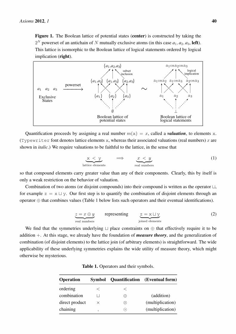
As applied to inference, each state of the world is associated, via isomorphism, with a statementabout the world. This results in a set of mutually exclusive statements, which we call atoms. Atoms arecombined through logical OR to form compound statements comprising the elements of a Boolean lattice(Figure 1, right), which is isomorphic to a Boolean lattice of sets (Figure 1, center). Although carryingdifferent interpretations, the mathematical structures are identical. Set inclusion “⊂” is equivalent tological implication “⇒”, which we abstract to lattice order “<”. It is a matter of choice whetherto include the null set ∅, equivalent to the logical absurdity ⊥. The set-based view is ontological incharacter and associated with Kolmogorov, while the logic-based view is epistemological in characterand associated with Cox.

Axioms 2012, 1 40

Figure 1. The Boolean lattice of potential states (center) is constructed by taking the2N powerset of an antichain of N mutually exclusive atoms (in this case a1, a2, a3, left).This lattice is isomorphic to the Boolean lattice of logical statements ordered by logicalimplication (right).

ExclusiveStates

a1 a2 a3

powerset−−−→

Boolean lattice ofpotential states

{a1,a2,a3}

{a1,a2} {a1,a3} {a2,a3}

{a1} {a2} {a3}

6

����

@@@I

����

@@@I 6

���� 6

@@@I

..

..6...

....�

......

.I

∅

subsetinclusion

∼

Boolean lattice oflogical statements

a1ORa2ORa3

a1ORa2 a1ORa3 a2ORa3

a1 a2 a3

6

����

@@@I

����

@@@I 6

���� 6

@@@I

..

..6...

....�

......

.I

⊥

logicalimplication

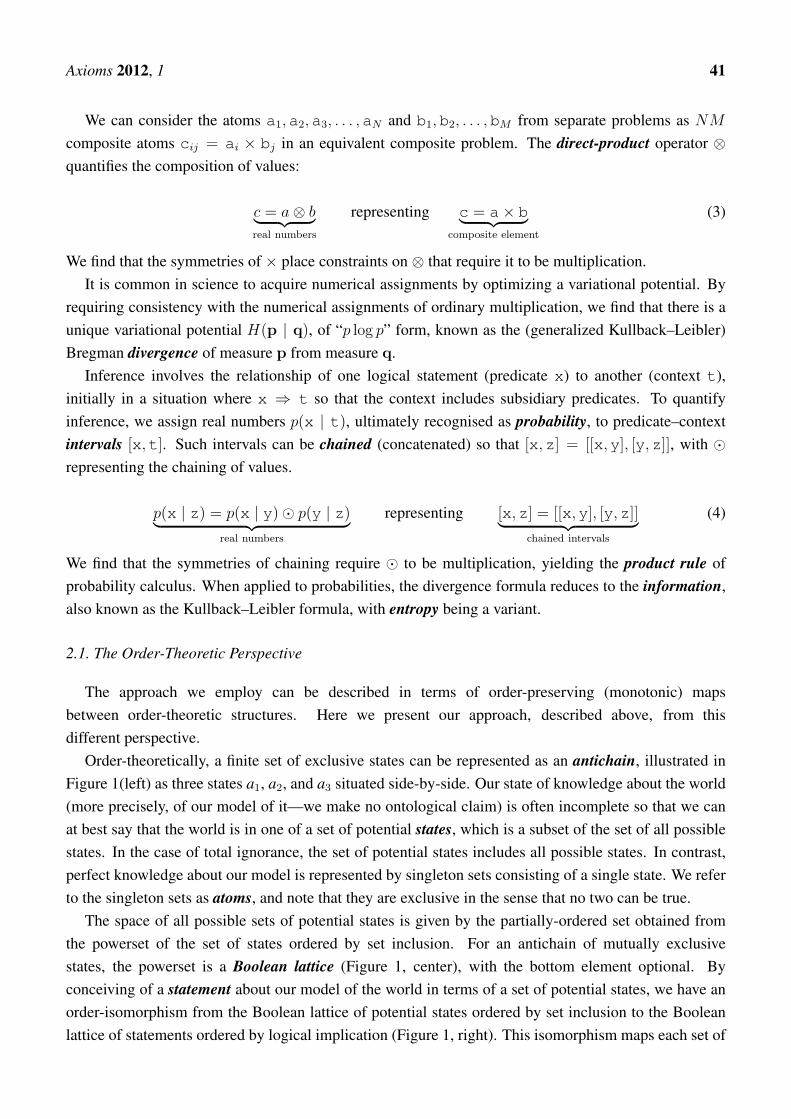
Quantification proceeds by assigning a real number m(x) = x, called a valuation, to elements x.(Typewriter font denotes lattice elements x, whereas their associated valuations (real numbers) x areshown in italic.) We require valuations to be faithful to the lattice, in the sense that

x < y︸ ︷︷ ︸lattice elements

=⇒ x < y︸ ︷︷ ︸real numbers

(1)

so that compound elements carry greater value than any of their components. Clearly, this by itself isonly a weak restriction on the behavior of valuation.

Combination of two atoms (or disjoint compounds) into their compound is written as the operator t,for example z = x t y. Our first step is to quantify the combination of disjoint elements through anoperator ⊕ that combines values (Table 1 below lists such operators and their eventual identifications).

z = x⊕ y︸ ︷︷ ︸real numbers

representing z = x t y︸ ︷︷ ︸joined elements

(2)

We find that the symmetries underlying t place constraints on ⊕ that effectively require it to beaddition +. At this stage, we already have the foundation of measure theory, and the generalization ofcombination (of disjoint elements) to the lattice join (of arbitrary elements) is straightforward. The wideapplicability of these underlying symmetries explains the wide utility of measure theory, which mightotherwise be mysterious.

Table 1. Operators and their symbols.

Operation Symbol Quantification (Eventual form)

ordering < <

combination t ⊕ (addition)direct product × ⊗ (multiplication)chaining , � (multiplication)

Axioms 2012, 1 41

We can consider the atoms a1,a2,a3, . . . ,aN and b1,b2, . . . ,bM from separate problems as NMcomposite atoms cij = ai × bj in an equivalent composite problem. The direct-product operator ⊗quantifies the composition of values:

c = a⊗ b︸ ︷︷ ︸real numbers

representing c = a× b︸ ︷︷ ︸composite element

(3)

We find that the symmetries of × place constraints on ⊗ that require it to be multiplication.It is common in science to acquire numerical assignments by optimizing a variational potential. By

requiring consistency with the numerical assignments of ordinary multiplication, we find that there is aunique variational potential H(p | q), of “p log p” form, known as the (generalized Kullback–Leibler)Bregman divergence of measure p from measure q.

Inference involves the relationship of one logical statement (predicate x) to another (context t),initially in a situation where x ⇒ t so that the context includes subsidiary predicates. To quantifyinference, we assign real numbers p(x | t), ultimately recognised as probability, to predicate–contextintervals [x,t]. Such intervals can be chained (concatenated) so that [x,z] = [[x,y], [y,z]], with �representing the chaining of values.

p(x | z) = p(x | y)� p(y | z)︸ ︷︷ ︸real numbers

representing [x,z] = [[x,y], [y,z]]︸ ︷︷ ︸chained intervals

(4)

We find that the symmetries of chaining require � to be multiplication, yielding the product rule ofprobability calculus. When applied to probabilities, the divergence formula reduces to the information,also known as the Kullback–Leibler formula, with entropy being a variant.

2.1. The Order-Theoretic Perspective

The approach we employ can be described in terms of order-preserving (monotonic) mapsbetween order-theoretic structures. Here we present our approach, described above, from thisdifferent perspective.

Order-theoretically, a finite set of exclusive states can be represented as an antichain, illustrated inFigure 1(left) as three states a1, a2, and a3 situated side-by-side. Our state of knowledge about the world(more precisely, of our model of it—we make no ontological claim) is often incomplete so that we canat best say that the world is in one of a set of potential states, which is a subset of the set of all possiblestates. In the case of total ignorance, the set of potential states includes all possible states. In contrast,perfect knowledge about our model is represented by singleton sets consisting of a single state. We referto the singleton sets as atoms, and note that they are exclusive in the sense that no two can be true.

The space of all possible sets of potential states is given by the partially-ordered set obtained fromthe powerset of the set of states ordered by set inclusion. For an antichain of mutually exclusivestates, the powerset is a Boolean lattice (Figure 1, center), with the bottom element optional. Byconceiving of a statement about our model of the world in terms of a set of potential states, we have anorder-isomorphism from the Boolean lattice of potential states ordered by set inclusion to the Booleanlattice of statements ordered by logical implication (Figure 1, right). This isomorphism maps each set of

Axioms 2012, 1 42

potential states to a statement, while mapping the algebraic operations of set union ∪ and set intersection∩ to the logical OR and AND, respectively.

The perspective provided by order theory enables us to focus abstractly on the structure of a Booleanlattice with its generic algebraic operations join ∨ and meet ∧. This immediately broadens the scopefrom Boolean to more general distributive lattices — the first fruit of our minimalist approach. Foradditional details on partially ordered sets and lattices in particular, we refer the interested reader to theclassic text by Birkhoff [3] or the more recent text by Davey & Priestley [4].

Quantification proceeds by assigning valuations m(x) = x to elements x, to form a real-valuedrepresentation. For this to be faithful, we require an order-preserving (monotonic) map between thepartial order of a distributive lattice and the total order of the chains that are to be found within. Thusx < y is to imply that x < y, a relationship that we call fidelity. The converse is not true: the total orderimposed by quantification must be consistent with but can extend the partial order of the lattice structure.

We write the combination of two atoms into a compound element (and more generally any two disjointcompounds into a compound element) as t, for example z = x t y. Derivation of the calculus ofquantification starts with this disjoint combination operator, where we find that its symmetries placeconstraints on its representation ⊕ that allow us the convention of ordinary addition “⊕ = +”. Thisbasic result generalizes to the standard join lattice operator ∨ for elements that (possibly having atomsin common) need not be disjoint, for which the sum rule generalizes to its standard inclusion/exclusionform [5], which involves the meet ∧ for any atoms in common.

There are two mathematical conventions concerning the handling the nothing-is-true null element⊥ atthe bottom of the lattice known as the absurdity. Some mathematicians opt to include the bottom elementon aesthetic grounds, whereas others opt to exclude it because of its paradoxical interpretation [4]. If itis included, its quantification is zero. Either way, fidelity ensures that other elements are quantified bypositive values that are positive (or, by elementary generalization, zero). At this stage, we already havethe foundation of measure theory.

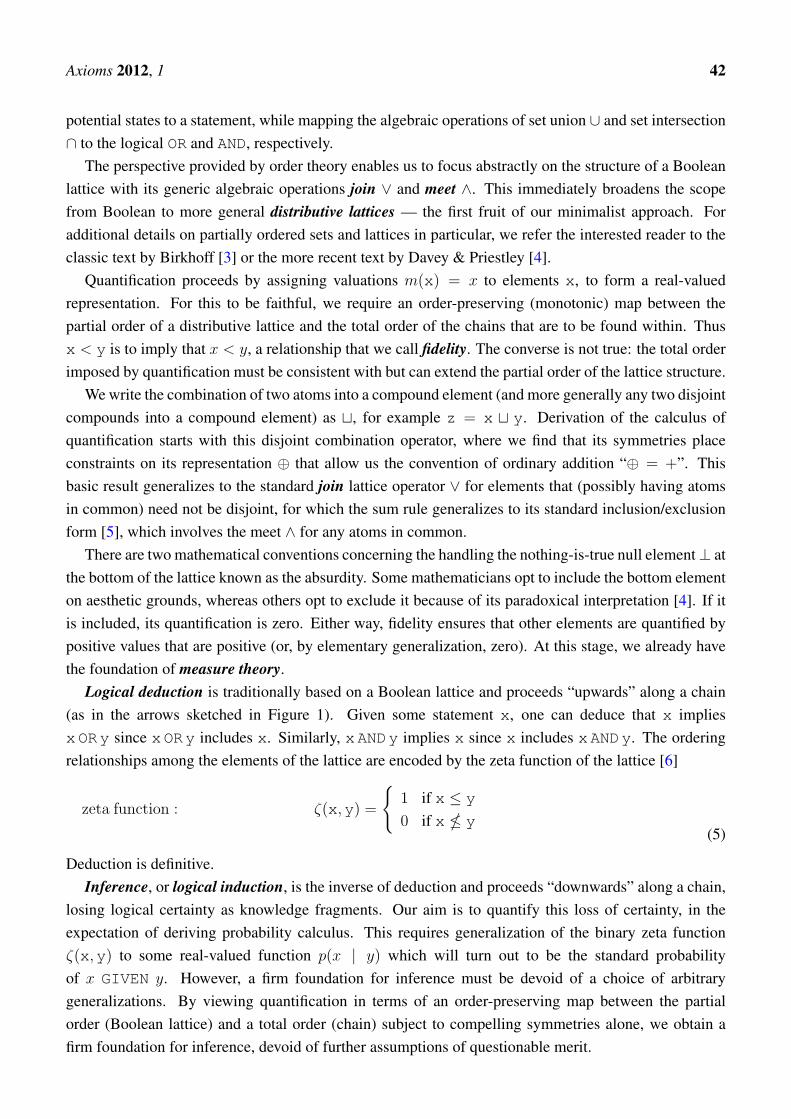
Logical deduction is traditionally based on a Boolean lattice and proceeds “upwards” along a chain(as in the arrows sketched in Figure 1). Given some statement x, one can deduce that x impliesxORy since xORy includes x. Similarly, xANDy implies x since x includes xANDy. The orderingrelationships among the elements of the lattice are encoded by the zeta function of the lattice [6]

zeta function : ζ(x,y) =

{1 if x ≤ y

0 if x � y(5)

Deduction is definitive.Inference, or logical induction, is the inverse of deduction and proceeds “downwards” along a chain,

losing logical certainty as knowledge fragments. Our aim is to quantify this loss of certainty, in theexpectation of deriving probability calculus. This requires generalization of the binary zeta functionζ(x,y) to some real-valued function p(x | y) which will turn out to be the standard probabilityof x GIVEN y. However, a firm foundation for inference must be devoid of a choice of arbitrarygeneralizations. By viewing quantification in terms of an order-preserving map between the partialorder (Boolean lattice) and a total order (chain) subject to compelling symmetries alone, we obtain afirm foundation for inference, devoid of further assumptions of questionable merit.

Axioms 2012, 1 43

By considering atoms (singleton sets, which are the join-irreducible elements of the Booleanlattice) as precise statements about exclusive states, and composite lattice elements (sets of severalexclusive states) as less precise statements involving a degree of ignorance, the two perspectives oflogic and sets, on which the Cox and Kolmogorov foundations are based, become united within theorder-theoretic framework.

In summary, the powerset comprises the hypothesis space of all possible statements that one canmake about a particular model of the world. Quantification of join using + is the sum rule of probabilitycalculus, and is required by adherence to the symmetries we list. It fixes the valuations assigned tocomposite elements in terms of valuations assigned to the atoms. Those latter valuations assigned tothe atoms remain free, unconstrained by the calculus. That freedom allows the calculus to apply toinference in general, with the mathematically-arbitrary atom valuations being guided by insight into aparticular application.

2.2. Commentary

Our results—the sum rule and divergence for measures, and the sum and product rules withinformation for probabilities—are standard and well known (their uniqueness perhaps less so). Thematter we address here is which assumptions are necessary and which are not. A Boolean lattice, after all,is a special structure with special properties. Insofar as fewer properties are needed, we gain generality.Wider applicability may be of little value to those who focus solely on inference. Yet, by showing thatthe basic foundations of inference have wider scope, we can thereby offer extra—and simpler—guidanceto the scientific community at large.

Even within inference, distributive problems may have relationships between their atoms such that notall combinations of states are allowed. Rather than extend a distributive lattice to Boolean by paddingit with zeros, the tighter framework immediately empowers us to work with the original problem in itsown right. Scientific problems (say, the propagation of particles, or the generation of proteins) are oftenheavily conditional, and it could well be inappropriate or confusing to go to a full Boolean lattice whena sparser structure is a more natural model.

We also confirm that commutativity is not a necessary assumption. Rather, commutativity of measureis imposed by the associativity and order required of a scalar representation. Conversely, systems that arenot commutative (matrices under multiplication, for example) cannot be both associative and ordered.

3. Symmetries

Here, we list the relevant symmetries on which our axioms are based. All are properties of distributivelattices, and our descriptions are styled that way so that a reader wary of further generality does not needto move beyond this particular, and important, example. However, one may note that not all the propertiesof a distributive lattice (such as commutativity of the join) are listed, which implies that these results areapplicable to a broader class of algebraic structures that includes distributive lattices.

Valuation assignments rank statements via an order-preserving map which we call fidelity .

Axioms 2012, 1 44

Symmetry 0 : x < y︸ ︷︷ ︸lattice elements

=⇒ x < y︸ ︷︷ ︸real numbers (6)

It is a matter of convention that we choose to order the valuations in the same sense as the lattice order(“more is bigger”). Reverse order would be admissible and logically equivalent, though less convenient.

In the specific case of Boolean lattices of logical statements, the binary ordering relation, representedgenerically by <, is equivalent to logical implication (⇒) between different statements, or equivalently,proper subset inclusion (⊂) in the powerset representation. Combination preserves order from the rightand from the left

Symmetry 1 : x < y =⇒

{x t z < y t zz t x < z t y (7)

for any z (a property that can be viewed as distributivity of t over <) on the grounds that ordering needsto be robust if it is to be useful. Combination is also taken to be associative

Symmetry 2 : (x t y) t z = x t (y t z) (8)

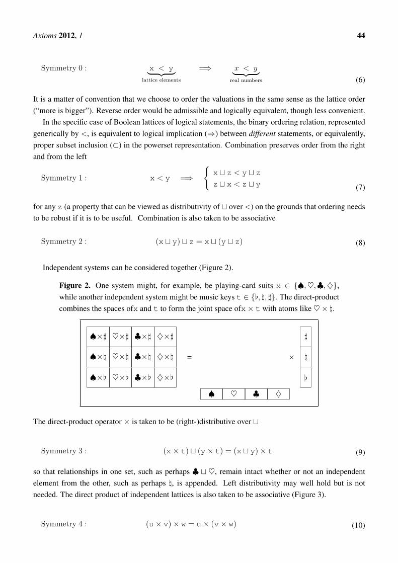
Independent systems can be considered together (Figure 2).

Figure 2. One system might, for example, be playing-card suits x ∈ {♠,♥,♣,♦},while another independent system might be music keys t ∈ {[, \, ]}. The direct-productcombines the spaces ofx and t to form the joint space ofx× t with atoms like ♥× \.

♠×[ ♥×[ ♣×[ ♦×[

♠×\ ♥×\ ♣×\ ♦×\

♠×] ♥×] ♣×] ♦×]

=

♠ ♥ ♣ ♦

×

[

\

]

The direct-product operator × is taken to be (right-)distributive over t

Symmetry 3 : (x× t) t (y× t) = (x t y)× t (9)

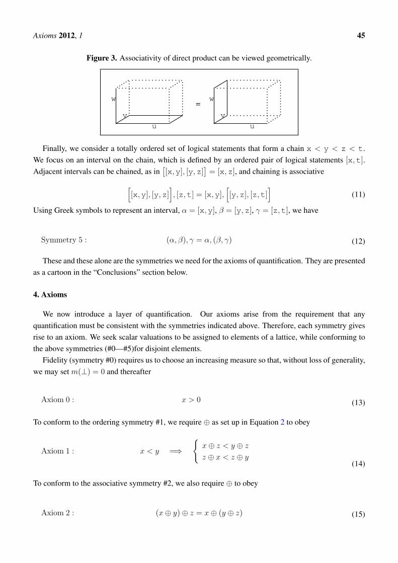
so that relationships in one set, such as perhaps ♣ t ♥, remain intact whether or not an independentelement from the other, such as perhaps \, is appended. Left distributivity may well hold but is notneeded. The direct product of independent lattices is also taken to be associative (Figure 3).

Symmetry 4 : (u× v)× w = u× (v× w) (10)

Axioms 2012, 1 45

Figure 3. Associativity of direct product can be viewed geometrically.

u

v

w

. . . . . . . . . . . . . . .. . . . . . . . . . . . . . .

......

......

""

"" ..

..

..

..

..

..

.

..

..

..

..

..

..

.

..

..

..

..

..

..

.

=

u

v

w

. . . . . . . . . . . . . . .

. . . . . . . . . . . . . . .

. . . . . . . . . . . . . . ."

" ......

......

"" ..

..

..

..

..

..

.

..

..

..

..

..

..

.

Finally, we consider a totally ordered set of logical statements that form a chain x < y < z < t.We focus on an interval on the chain, which is defined by an ordered pair of logical statements [x,t].Adjacent intervals can be chained, as in

[[x,y], [y,z]

]= [x,z], and chaining is associative[

[x,y], [y,z]], [z,t] = [x,y],

[[y,z], [z,t]

](11)

Using Greek symbols to represent an interval, α = [x,y], β = [y,z], γ = [z,t], we have

Symmetry 5 : (α, β), γ = α, (β, γ) (12)

These and these alone are the symmetries we need for the axioms of quantification. They are presentedas a cartoon in the “Conclusions” section below.

4. Axioms

We now introduce a layer of quantification. Our axioms arise from the requirement that anyquantification must be consistent with the symmetries indicated above. Therefore, each symmetry givesrise to an axiom. We seek scalar valuations to be assigned to elements of a lattice, while conforming tothe above symmetries (#0—#5)for disjoint elements.

Fidelity (symmetry #0) requires us to choose an increasing measure so that, without loss of generality,we may set m(⊥) = 0 and thereafter

Axiom 0 : x > 0 (13)

To conform to the ordering symmetry #1, we require ⊕ as set up in Equation 2 to obey

Axiom 1 : x < y =⇒

{x⊕ z < y ⊕ zz ⊕ x < z ⊕ y

(14)

To conform to the associative symmetry #2, we also require ⊕ to obey

Axiom 2 : (x⊕ y)⊕ z = x⊕ (y ⊕ z) (15)

Axioms 2012, 1 46

These equations are to hold for arbitrary values x, y, z assigned to the disjoint x, y, z. Appendix Awill show that these order and associativity axioms are necessary and sufficient to determine the additivecalculus of measure.

To conform to the distributive symmetry #3, we require ⊗ as set up in Equation 3 to obey

Axiom 3 : (x⊗ t)⊕ (y ⊗ t) = (x⊕ y)⊗ t (16)

for disjoint x and y combined with any t from the second lattice. Presence of t may change themeasures, but does not change their underlying additivity. To conform to the associative symmetry #4,we also require ⊗ to obey

Axiom 4 : (u⊗ v)⊗ w = u⊗ (v ⊗ w) (17)

These axioms determine the multiplicative form of ⊗ and also lead to a unique divergence betweenmeasures.

To conform to the associative symmetry #5, we require � as set up in Equation 4 to obey

Axiom 5 :(p(α)� p(β)

)� p(γ) = p(α)�

(p(β)� p(γ)

)(18)

where α = [x,y], β = [y,z], γ = [z,t] are individual steps concatenated along the chain α, β, γ, whichis [[x,y], [y,z], [z,t]] = [x,t]. This final axiom will let us pass from measure to probability and Bayes’theorem, and from divergence to information and entropy. For each operator (Table 1), the eventual formsatisfies all relevant axioms, which assures existence. Uniqueness remains to be demonstrated.

5. Measure

Preliminary to investigating probability, we attend to the foundation of measure.

5.1. Disjoint arguments

According to the scalar associativity theorem (Appendix A), an operator ⊕ obeying axioms 1 and 2exists and can without loss of generality be taken to be addition +, giving the sum rule.

Sum rule : x⊕ y = x+ y (19)

Commutativity x ⊕ y = y ⊕ x, though not explicitly assumed, is an unsurprising property.In accordance with fidelity (axiom 0), element values are strictly positive x > 0. In this form,positive-valued valuation m(x) = x of lattice elements is known as a measure. If the null elementis included as the bottom of the lattice, it has zero value.

Axioms 2012, 1 47

Whilst we are free to adopt additivity as a convenient convention, we are also free to adopt anyorder-preserving regrade Θ for which the rule would be

x⊕ y = Θ−1(

Θ(x) + Θ(y))

(20)

This carries no extra generality because this form can be reverted to additivity by applying Θ, but weneed such alternative grading later to avoid inconsistency between different assignments. There is noother freedom. If the linear form of sum rule is to be maintained, the only freedom is linear rescalingΘ(x) = Kx, with K > 0 to retain positivity.

Measure theory (see for example [7]) is usually introduced with additivity (countably additive orσ-additive) and non-negativity as “obvious” basic assumptions, with emphasis on the technical controlof infinity in unbounded applications. Here we emphasize the foundation, and discover the reason whymeasure theory is constructed as it is. The symmetries of combination require it. Any other formulationwould break these basic properties of associativity and order, and would not yield a widely useful theory.

5.2. Arbitrary Arguments

For elements x and y that need not be disjoint, their join∨ is defined as comprising all their constituentatoms counted once only, and the meet ∧ as comprising those atoms they have in common. In inference,∨ is logical OR and ∧ is logical AND.

By putting x = u t v and y = v t w for disjoint u,v,w, we reach the general “inclusion/exclusion”sum rule for arbitrary x and y

m(x ∨ y) +m(x ∧ y) = m(x) +m(y) (21)

Commutativity of join and meet follow:

m(x ∨ y) = m(y ∨ x) , m(x ∧ y) = m(y ∧ x) . (22)

5.3. Independence

From the associativity of direct product (axiom 4), the associativity theorem (Appendix A again)assures the existence of an additivity relationship of the form

Θ(x⊗ t) = Θ(x) + Θ(t) (23)

for some invertible function Θ of the measures x = m(x), t = m(t) and x⊗ t = m(x×t). We can notproceed as before to re-grade in terms of Θ(m) to supersede m, because we are already using additivity

x⊗ t+ y ⊗ t = (x+ y)⊗ t (24)

(axiom 3, distributivity of ⊗ over ⊕=+) to define the grade. Instead, we require consistency with thesum-rule behavior for x⊗ t and y ⊗ t. Defining Ψ = Θ−1 gives, term by term,

Ψ(ξ + τ) + Ψ(η + τ) = Ψ(ζ(ξ, η) + τ) (25)

Axioms 2012, 1 48

where

ξ = Θ(x) , η = Θ(y) , ζ = Θ(x+ y) , τ = Θ(t) . (26)

Among these variables, ξ, η, τ are independent, but (through the sum rule), ζ depends on ξ and η butnot τ . This is the product equation. By definition, Ψ returns a measure, so it is positive.

The product theorem (Appendix B) shows Θ to be logarithmic, with Equation 23 reading

1

Alog

x⊗ tC

=1

Alog

x

C+

1

Alog

t

C(27)

with A and C universal constants (A cancelling out), and C being positive. The obvious conventionC = 1 loses no generality, and shows ⊗ to be simple multiplication

Direct-product rule : x⊗ t = x t (28)

Measures are required to multiply, because of associativity of direct product, and the “⊗ t” operation isrepresented by “scale by t”. This is consistent with linear rescaling (here depending on the second factort) being the only allowed freedom for the measure assigned to the first factor x.

6. Variation

Variational principles are common in science—minimum energy for equilibrium, Hamilton’sprinciple for dynamics, maximum entropy for thermodynamics, and so on—and we seek one formeasures. The aim is to discover a variational potential H(m) whose constrained minimum allowsthe valuations m = (m1,m2, . . . ,mN) of N atoms to be assigned subject to appropriate constraints ofthe form f(m) = constant. (The vectors which appear in this section are shown in bold-face font.)

The variational potential is required to be general, applying to arbitrary constraints. Just like valuesthemselves, constraints on individual atom values can be combined into compound constraints thatinfluence several values: indeed the constraints could simply be imposition of definitive values. Suchcombination allows a Boolean lattice, entirely analogous to Figure 1, to be developed from individualatomic constraints. The variational potential H is to be a valuation on the measures resulting from theseconstraints, combination being represented by some operator © so that

H(x WITH y) = H(x)©H(y) (29)

for constraints acting on disjoint atoms or compounds.Adding extra constraints always increases H , otherwise the variational requirement would be broken,

so H must be faithful to chaining in the lattice.

x < y︸ ︷︷ ︸chained

=⇒ H(x) < H(y)︸ ︷︷ ︸real numbers

(30)

We also have order

H(x) < H(y) =⇒

{H(x)©H(z) < H(y)©H(z)

H(z)©H(x) < H(z)©H(y)(31)

Axioms 2012, 1 49

because if y is a “harder” constraint than x (meaning H(y) > H(x)), that ranking should not be affectedby some other constraint on something else. Associativity(

H(x)©H(y))©H(z) = H(x)©

(H(y)©H(z)

)(32)

is likewise required and expresses the combination of three constraints. It would also be natural to assumecommutativity, H(x)©H(y) = H(y)©H(x), but that is not necessary because we already recognizeEquations 30–32 as our axioms 0, 1, 2. Hence, using Appendix A again, there exists a “© = +” gradeon which H is additive.

H(m) =∑

atoms i

Hi(mi) (33)

We have now justified additivity, thus filling a gap in traditional accounts of the calculus of variations.Under perturbation, the minimization requirement is

δH(m) ≥ 0 when δf1(m) = δf2(m) = · · · = 0 (34)

The standard “⊕ = +” form of the sum rule happens to be continuous and differentiable, so is applicableto valuation of systems that differ arbitrarily little. We adopt it, and can then justifiably require thevariational potential to be valid for arbitrarily small perturbations:

dH(m) = 0 when df1(m) = df2(m) = · · · = 0 (35)

This limit Equation 35 is weaker than the original Equation 34 not only because of the restricted context,but also because the nature of the extremum (maximum or minimum or saddle) is lost in the discardedsecond-order effects. However, it still needs to be satisfied. It also shows that any variational potentialmust by its nature be differentiable at least once.

One now invents supposedly constant “Lagrange multiplier” coefficients λ1, λ2, . . . and considerswhat appears at first to be the different problem of solving

d(H(m)− λ1f1(m)− λ2f2(m)− . . .

)= 0 under arbitrary perturbation (36)

for m. Clearly, Equation 36 is equivalent to Equation 35 for perturbations that happen to hold the f ’sconstant (df = 0). However, the values those f ’s take may well be wrong. The trick is to choose the λ’sso that the f ’s take their correct constraint values. That being done, Equation 36 solves the variationalproblem Equation 35.

Let the application be two-dimensional, x-by-y, in the sense of applying to values m(x × y) ofelements on a direct-product lattice. Suppose we have x-dependent constraints that yield m(x) = mx

on one factor (say the card suits in Figure 2 above), and similar y-dependent constraints that yieldm(y) = my on the other factor (say music keys in Figure 2). Both factors being thus controlled, theirdirect-product is implicitly controlled by the those same constraints. Here, we already know the targetvalue m(x × y) = mxmy from the direct-product rule Equation 28. Hence the variational assignmentfor the particular value m(x× y) derives from

H ′xy(mxmy) = λ1f1(mx) + λ2f2(my) (37)

Axioms 2012, 1 50

(where ′ indicates derivative). The variational theorem (Appendix C) gives the solution of this functionalequation as

Hi(mi) = Ai +Bimi + Ci(mi logmi −mi) (38)

for the individual valuation being considered, where Ai, Bi, Ci are constants. Combining all theatoms yields

H(m) =∑

atoms i

(Ai +Bimi + Ci(mi logmi −mi)

)(39)

The coefficient Ci represents the intrinsic importance of atom ai in the summation, but usually theatoms are a priori equivalent so that the C’s take a common value. The scaling of a variational potentialis arbitrary (and is absorbed in the Lagrange multipliers), so we may set C = 1, ensuring that H hasa minimum rather than a maximum. Alternatively, C = −1 would ensure a maximum. However, thesettings of A and B depend on the application.

6.1. Divergence and Distance

One use of H is as a quantifier of the divergence of destination values w from source values u thatexisted before the constraints that led to w were applied. For this, we set C = 1 to get a minimum,Bi = − log ui to place the unconstrained minimizing w at u, and Ai = ui to make the minimum valuezero. This form is

Divergence : H(w | u) =∑

atoms i

(ui − wi + wi log(wi/ui)

)(40)

This formula is unique: none other has the properties Equations 33,37 that elementary applicationsrequire. Equivalently, any different formula would give unjustifiable answers in those applications.Plausibly, H is non-negative, H(w | u) ≥ 0 with equality if and only if w = u, so that it usefullyquantifies the separation of destination from source.

In general, H obeys neither commutativity nor the triangle inequality, H(w | u) 6= H(u | w) andH(w | u) 6≤ H(w | v) + H(v | u). Hence it cannot be a geometrical “distance”, which is requiredto have both those properties. In fact, there is no definition of geometrical measure-to-measure distancethat obeys the basic symmetries, because H is the only candidate, and it fails.

Here again we see our methodology yielding clear insight. “From–to” can be usefully quantified, but“between” cannot. A space of measures may have connectedness, continuity, even differentiability, butit cannot become a metric space and remain consistent with its foundation.

In the limit of many small values, H admits a continuum limit

H(w | u) =

∫ (u(θ)− w(θ) + w(θ) log(w(θ)/u(θ))

)dθ (41)

The constraints that force a measure away from the original source may admit several destinations, butminimizing H is the unique rule that defines a defensibly optimal choice. This is the rationale behindmaximum entropy data analysis [8].

Axioms 2012, 1 51

7. Probability Calculus

In inference, we seek to impose on the hypothesis space a quantified degree of implication p(x | t),to represent the plausibility of predicate x conditional on current knowledge that excludes all hypothesesoutside the stated context t. This is accomplished via a bivaluation, which is a functional that takes apair of lattice elements to a real number. This bivaluation should depend on both x (obviously) and t(otherwise it would be just the measure assigned to x). The natural conjecture is that probability shouldbe identified with a normalized measure, and we proceed to prove this—measures can have arbitrarytotal but probabilities will (according to standard convention) sum to unity.

At the outset, though, we simply wish to set up a bivaluation for predicate x within context t.

7.1. Chained Arguments

Within given context t, we require p(x | t) to have the order and associative symmetries #1 and #2that define a measure. Consequently, p obeys the sum rule

p(x t y | t) = p(x | t) + p(y | t) (42)

for disjoint x and y with x t y < t. It is the dependence on t that remains to be determined.Associativity of chaining (axiom 5) for a < b < c < d is represented by(

p(a | b)︸ ︷︷ ︸p(α)

� p(b | c)︸ ︷︷ ︸p(β)︸ ︷︷ ︸

p(α,β)

)� p(c | d)︸ ︷︷ ︸

p(γ)

= p(a | b)︸ ︷︷ ︸p(α)

�(p(b | c)︸ ︷︷ ︸

p(β)

� p(c | d)︸ ︷︷ ︸p(γ)︸ ︷︷ ︸

p(β,γ)

)(43)

We do not have commutativity, (α, β) = [[a,b], [b,c]] = [a,c] not being the same as (β, α) (which ismeaningless), but we do have associativity and we do have order along the chain. By the associativitytheorem,� exists and there is a scale on which it is simple addition. However, we can not regrade to thatscale and discard the original because we have already fixed the grade of p to be additive with respect toits first argument. Instead, we infer additivity on some other grade Θ(p)

Θ(p(a | c)︸ ︷︷ ︸p(α)�p(β)

)= Θ

(p(a | b)︸ ︷︷ ︸

p(α)

)+ Θ

(p(b | c)︸ ︷︷ ︸

p(β)

)(44)

required to be consistent with the sum-rule behavior of p. Defining Ψ = Θ−1 gives

p(a | c)︸ ︷︷ ︸p(α)�p(β)

= Ψ(

Θ(p(a | b)︸ ︷︷ ︸p(α)

) + Θ(p(b | c)︸ ︷︷ ︸p(β)

))

(45)

Substituting this in the sum rule Equation 42, term by term, yields the same “product Equation” 25

Ψ(ζ(ξ, η) + τ) = Ψ(ξ + τ) + Ψ(η + τ) (46)

as before, where

ξ = Θ(p(x | z)

), η = Θ

(p(y | z)

), ζ = Θ

(p(x t y | z)

), τ = Θ

(p(z | t)

). (47)

Axioms 2012, 1 52

Through the sum rule, ζ depends as shown on ξ and η but not τ . The independent variables are ξ, η, τ .The solution (Appendix B again) shows Θ to be logarithm, so that � was multiplication and

p(x | z) = p(x | y) p(y | z) /C (48)

in which p (positive by virtue of being a measure on predicates) takes the sign of a universal constant C.Without loss of generality, we assign the scale of p by fixing C = 1, giving the standard product rule forconditioning.

Chain-product rule : p(x | z) = p(x | y) p(y | z) (49)

7.2. Arbitrary Arguments

The chain-product rule, which as written above is valid for any chain, can be generalized toaccommodate arbitrary elements. This is accomplished by noting that x ∧ y = x in a chain wherex < y, so that p(x ∧ y | y) = p(x | y). The general form

p(a ∧ b | c) = p(a | b ∧ c) p(b | c) (50)

follows by observing that x = a ∧ b ∧ c, y = b ∧ c and z = c form a chain and hence are subject tothe chain rule.

The special case p(t | t) = 1 is obtained by setting y = z = t in the chain-product rule. For anyx ≤ t, ordering requires p(x | t) ≤ p(t | t) = 1, so that the range of values is 0 ≤ p ≤ 1 and werecognize p as probability, hereafter denoted Pr.

Probability calculus is now proved:

Range

Sum rule

Chain-product

0 = Pr(⊥ | t) < Pr(x | t) ≤ Pr(t | t) = 1

Pr(x ∨ y | t) + Pr(x ∧ y | t) = Pr(x | t) + Pr(y | t)

Pr(x ∧ y | t) = Pr(x | y ∧ t) Pr(y | t)

The top element of the current lattice, t, is the (provisional) truth, often written >.From the commutativity Pr(x∧y | t) = Pr(y∧x | t) associated with ∧, we obtain Bayes’ Theorem

Pr(x | θ ∧ t) Pr(θ | t) = Pr(θ | x ∧ t) Pr(x | t) (51)

which can be simplified by making the common context implicit and writing

Pr(x | θ)︸ ︷︷ ︸Likelihood

Pr(θ)︸ ︷︷ ︸Prior

= Pr(θ | x)︸ ︷︷ ︸Posterior

Pr(x)︸ ︷︷ ︸Evidence

‖ t (52)

to relate data x and parameter θ (with context t understood). Do not misinterpret the abbreviatednotation. Probability is always and necessarily, by construction, a bivaluation that assigns a real numberto a pair of elements in a Boolean lattice. In addition, one does not need to differentiate between

Axioms 2012, 1 53

likelihood, prior, posterior, and evidence by giving each one a different notation. The terms that compriseBayes’ Theorem represent the same bivaluation applied to different pairs of elements.

7.3. Probability as a Ratio

The equations of probability calculus (range, sum rule, and chain-product rule) can all be subsumedin the single expression

Pr(x | t) =m(x ∧ t)

m(t)∀x, ∀t 6= ⊥ (53)

for probability as a ratio of measures. Thus the calculus of probability is nothing more than theelementary calculus of proportions of measure. As anticipated, within its context t, a probabilitydistribution is simply the shape of the confined measure, automatically normalized to unit mass.

This is, essentially, the original discredited frequentist definition (see [9]) of probability, as the ratioof number of successes to number of trials. However, it is here retrieved at an abstract level, whichbypasses the catastrophic difficulties of literal frequentism when faced with isolated non-reproduciblesituations. Just as ordinary addition is forced for measures in [0,∞), so ordinary proportions in [0, 1] areforced for probability calculus.

Whereas the sum rule for measure and probability generalizes to the inclusion/exclusion form forgeneral elements which need not be disjoint, so does the ratio form of probability allow generalizationfrom intervals [3] to generalized intervals, consisting of arbitrary pairs [x,t] which need not be in achain. The bivaluation form Equation 53 still holds but now represents a general degree of implicationbetween arbitrary elements.

8. Information and Entropy

Here, we take special cases of the variational potential H , appropriate for probability distributionsinstead of arbitrary measures.

8.1. Information

Within a given context, probability is a measure, normalized to unit mass. The divergence H ofdestination probability p from source probability q then simplifies to

Information : H(p | q) =∑k

pk logpkqk

(54)

In statistics, this is known as the Kullback–Leibler formula [10].If the final destination is a fully determined state, with a single p equal to 1 while all the others are

necessarily 0, then we have the extreme case

H(p | q) = − log qk when pk = 1 . (55)

Axioms 2012, 1 54

This represents the information gained on acquiring the knowledge that the specific k wastrue—equivalently the surprise at finding k instead of any available alternative. Generally, H is theamount of compression (logarithmically, with respect to the source) induced by the constraints thatmodulate source into destination.

In the limit of many small values, H admits a continuum limit

H(p | q) =

∫p(x) log

p(x)

q(x)dx (56)

sometimes (with a minus sign) known as the cross-entropy.

8.2. Entropy

The variational potential

H(p) =∑k

(Ak +Bkpk + C(pk log pk − pk)

)(57)

can also quantify uncertainty. For this, we require zero uncertainty when one probability value equals to1 (definitely present) and all the others are necessarily 0 (definitely not present). This is accomplishedby setting Ak = 0 and Bk = C. Setting C = −1 gives the conventional scale, and yields

Entropy : S(p) = −∑k

pk log pk

(58)

We call this “entropy”, and give it a separate symbol S as well as a separate name, to distinguish it fromthe previous “information” special case of divergence.

Entropy happens to be the expectation value of the information gained by deciding on one particularcell instead of any of the others in a partition.

S(p) =⟨− log pk

⟩k

(59)

It is a function of the partitioning as well as the probability distribution, which is why it does not have acontinuum limit. Plausibly, entropy has the following three properties:

• S is a continuous function of its arguments.• If there are n equal choices, so that pk = 1/n, then S is monotonically increasing in n.• If a choice is broken down into subsidiary choices, then

S adds according to probabilistic expectation, meaningS(p1, p2, p3) = S(p1, p2+p3) + (p2+p3)S(p2, p3).

These are the three properties from which Shannon [11] originally proved the entropy formula. Here, wesee that those properties, like that formula, are inevitable consequences of seeking a variational quantityfor probabilities.

Information and entropy are near synonyms, and are often used interchangeably. As seen here, though,entropy S is different from H . It is a property of just one partitioned probability distribution, it has amaximum not a minimum, and it does not have a continuum limit. Its least value, attained when a single

Axioms 2012, 1 55

probability is 1 and all the others are 0, is zero. Its value generally diverges upwards as the partitioningdeepens, whereas H usually tends towards a continuum limit.

9. Conclusions

9.1. Summary

We start with a set {a1,a2,a3, . . . ,aN} of “atomic” elements which in inference represent the mostfundamental exclusive statements we can make about the states (of our model) of the world. Atomscombine to form a Boolean lattice which in inference is called the hypothesis space of statements. Thisstructure has rich symmetry, but other applications may have less and we have selected only what weneeded, so that our results apply more widely and to distributive lattices in particular. The minimalassumptions are so simple that they can be drawn as the cartoon below (Figure 4).

Axiom 1 represents the order property that is required of the combination operator t. Axiom 2 saysthat valuation must conform to the associativity of t. These axioms are compelling in inference. Bythe associativity theorem (Appendix A — see the latter part for a proof of minimality) they require thevaluation to be a measure m(x), with t represented by addition (the sum rule). Any 1:1 regrading isallowed, but such change alters no content so that the standard linearity can be adopted by convention.This is the rationale behind measure theory.

The direct product operator × that represents independence is distributive (axiom 3) and associative(axiom 4), and consequently independent measures multiply (the direct-product rule). There is thena unique form of variational potential for assigning measures under constraints, yielding a uniquedivergence of one measure from another.

Probability Pr(x | t) is to be a bivaluation, automatically a measure over predicate x within anyspecified context t. Axiom 5 expresses associativity of ordering relations (in inference, implications)and leads to the chain-product rule which completes probability calculus. The variational potentialdefines the information (Kullback–Leibler) carried by a destination probability relative to its source, andalso yields the Shannon entropy of a partitioned probability distribution.

9.2. Commentary

We have presented a foundation for inference that unites and significantly extends the approaches ofKolmogorov [2] and Cox [1], yielding not just probability calculus, but also the unique quantification ofdivergence and information. Our approach is based on quantifying finite lattices of logical statementsin such a way that quantification satisfies minimal required symmetries. This generalizes algebraicimplication, or equivalently subset inclusion, to a calculus of degrees of implication. It is remarkablethat the calculus is unique.

Our derivations have relied on a set of explicit axioms based on simple symmetries. In particular, wehave made no use of negation (NOT), which in applications other than inference may well not be present.Neither have we assumed any additive or multiplicative behavior (as did Kolmogorov [2], de Finetti [12],and Dupre & Tipler [13]). On the contrary, we find that sum and product rules follow from elementarysymmetry alone.

Axioms 2012, 1 56

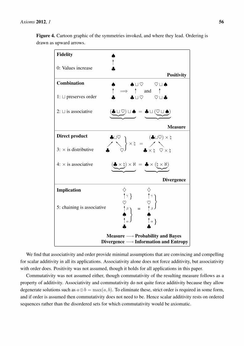
Figure 4. Cartoon graphic of the symmetries invoked, and where they lead. Ordering isdrawn as upward arrows.

Fidelity

0: Values increase

♠6

♣Positivity

Combination

1: t preserves order

♠6

♣=⇒

♠t♥6

♣ t♥and

♥ t♠6

♥ t♣

2: t is associative (♣ t♥︸ ︷︷ ︸) t ♠︸ ︷︷ ︸ = ♣ t (♥ t♠︸ ︷︷ ︸)︸ ︷︷ ︸Measure

Direct product

3: × is distributive

♣t♥

♣��� @@I

♥

}× \ =

(♣t♥)× \

♣× \��� @@I

♥× \

4: × is associative (♣× \︸ ︷︷ ︸)× ℵ︸ ︷︷ ︸ = ♣× (\× ℵ︸ ︷︷ ︸)︸ ︷︷ ︸Divergence

Implication

5: chaining is associative

♦6γ

♥6β

♠6α

♣

}}}

=

♦6γ

♥6β

♠6α

♣

}}

}

Measure −→ Probability and BayesDivergence −→ Information and Entropy

We find that associativity and order provide minimal assumptions that are convincing and compellingfor scalar additivity in all its applications. Associativity alone does not force additivity, but associativitywith order does. Positivity was not assumed, though it holds for all applications in this paper.

Commutativity was not assumed either, though commutativity of the resulting measure follows as aproperty of additivity. Associativity and commutativity do not quite force additivity because they allowdegenerate solutions such as a⊕b = max(a, b). To eliminate these, strict order is required in some form,and if order is assumed then commutativity does not need to be. Hence scalar additivity rests on orderedsequences rather than the disordered sets for which commutativity would be axiomatic.

Axioms 2012, 1 57

Associativity + Order =⇒ Additivity allowed =⇒ Commutativity

Associativity alone 6=⇒ Additivity allowed

Associativity + Commutativity 6=⇒ Additivity allowed

Aczel [14] assumes order in the form of reducibility, and he too derives commutativity. However, hisanalysis assumes the continuum limit already attained, which requires him to assume continuity.

Associativity + Order + Continuity =⇒ Additivity allowed =⇒ Commutativity

Our constructivist approach uses a finite environment in which continuity does not apply, and proceedsdirectly to additivity. Here, continuity and differentiability are merely emergent properties of + as thecontinuum limit is approached by allowing arbitrarily many atoms of different type.

Yet there can be no requirement of continuity, which is merely a convenient convention. For example,re-grading could take the binary representations of standard arguments (101.0112 representing 53

8) and

interpret them in base-3 ternary (with 101.0113 representing 10 427

), so that Θ(10 427

) = 538. Valuation

becomes discontinuous everywhere, but the sum rule still works, albeit less conveniently. Indeed, nofinite system can ever demonstrate the infinitesimal discrimination that defines continuity, so continuitycannot possibly be a requirement of practical inference.

At the cost of lengthening the proofs in the appendices, we have avoided assuming continuity ordifferentiability. Yet we remark that such infinitesimal properties ought not influence the calculus ofinference. If they did, those infinitesimal properties would thereby have observable effects. But detectingwhether or not a system is continuous at the infinitesimal scale would require infinite information,which is never available. So assuming continuity and differentiability, had that been demanded by thetechnicalities of mathematical proof (or by our own professional inadequacy), would in our view havebeen harmless. As it happens, each appendix touches on continuity, but the arguments are appropriatelyconstructed to avoid the assumption, so any potential controversy over infinite sets and the role of thecontinuum disappears.

Other than reversible regrading, any deviation from the standard formulas must inevitably contradictthe elementary symmetries that underlie them, so that popular but weaker justifications (e.g.,de Finetti [12]) in terms of decisions, loss functions, or monetary exchange can be discarded asunnecessary. In fact, the logic is the other way round: such applications must be cast in terms of theunique calculus of measure and probability if they are to be quantified rationally. Indeed, we holdgenerally that it is a tactical error to buttress a strong argument (like symmetry) with a weak argument(like betting, say). Doing that merely encourages a skeptic to sow confusion by negating the weakargument, thereby casting doubt on the main thesis through an illogical impression that the strongargument might have been circumvented too.

Finally, the approach from basic symmetry is productive. Goyal and ourselves [15] have used justthat approach to show why quantum theory is forced to use complex arithmetic. Long a deep mystery,the sum and product rules of complex arithmetic are now seen as inevitably necessary to describe thebasic interactions of physics. Elementary symmetry thus brings measure, probability, information andfundamental physics together in a remarkably unified synergy.

Axioms 2012, 1 58

Acknowledgements

The authors would like to thank Seth Chaikin, Janos Aczel, Ariel Caticha, Julian Center, PhilipGoyal, Steve Gull, Jeffrey Jewell, Vassilis Kaburlasos, Carlos Rodrıguez, and a thoughtful anonymousreviewer. KHK was supported in part by the College of Arts and Sciences and the College of Computingand Information of the University at Albany, NASA Applied Information Systems Research Program(NASA NNG06GI17G) and the NASA Applied Information Systems Technology Program (NASANNX07AD97A). JS was supported by Maximum Entropy Data Consultants Ltd.

References

1. Cox, R.T. Probability, frequency, and reasonable expectation. Am. J. Phys. 1946, 14, 1–13.2. Kolmogorov, A.N. Foundations of the Theory of Probability, 2nd English ed.; Chelsea: New

York, NY, USA, 1956.3. Birkhoff, G. Lattice Theory; American Mathematical Society: Providence, RI, USA, 1967.4. Davey, B.A.; Priestley, H.A. Introduction to Lattices and Order; Cambridge University Press:

Cambridge, UK, 2002.5. Klain, D.A.; Rota, G.-C. Introduction to Geometric Probability; Cambridge University Press:

Cambridge, UK, 1997.6. Knuth, K.H. Deriving Laws from Ordering Relations. In Bayesian Inference and Maximum

Entropy Methods in Science and Engineering; Erickson, G.J., Zhai, Y., Eds.; Jackson: Hole, WY,USA, 2003.

7. Halmos, P.R. Measure Theory; Springer: Berlin/Heidelberg, Germany; 1974.8. Gull, S.F.; Skilling, J. Maximum entropy method in image processing. IEE Proc. 131F, 646–659.9. Von Mises, R. Probability, Statistics, and Truth; Dover: Mineola, NY, USA, 1981.

10. Kullback, S.; Leibler, R.A. On information and sufficiency. Ann. Math. Statist. 1951, 22, 79–86.11. Shannon, C.F. A mathematical theory of communication. Bell Syst. Tech. J. 1948, 27, 379–423,

623–656.12. De Finetti, B. Theory of Probability, Vol. I and Vol. II; John Wiley and Sons: New York, NY,

USA, 1974.13. Dupre, M.J.; Tipler, F.J. New axioms for rigorous Bayesian probability. Bayesian Anal. 2009,

4, 599–606.14. Aczel, J. Lectures on Functional Equations and Their Applications; Academic Press: New York,

NY, USA, 1966.15. Goyal, P.; Knuth, K.H.; Skilling, J. Origin of complex quantum amplitudes and Feynman’s rules.

Phys. Rev. A 2010, 81, 022109.

A. Appendix A: Associativity Theorem

Atoms x, y, z,. . . , or disjoint lattice elements more generally, are to be assigned valuations x, y, z, . . . .If valuations coincide (though other marks may differ), such atoms are said to be of the same type. Weallow arbitrarily many atoms of arbitrarily many types. Our proof is constructive, with combinations

Axioms 2012, 1 59

built as sequences of atoms appended one at a time, x t y t . . . having valuation x ⊕ y ⊕ . . . . Theconsequent stand-alone derivation is rather long, but avoids making what would in our finite environmentbe an unnatural assumption of continuity. We also avoid assuming that an inverse to combination exists.

We merely assume order (axiom 1)

Axiom 1a :

Axiom 1b :x < y =⇒

{x⊕ z < y ⊕ zz ⊕ x < z ⊕ y

and associativity (axiom 2)

Axiom 2 : (x⊕ y)⊕ z = x⊕ (y ⊕ z)

Theorem:

Axiom 1 (order) and axiom 2 (associativity) imply that

x⊕ y = Θ−1(

Θ(x) + Θ(y))

for any order-preserving regrade Θ of “⊕ = +” applied to scalar values.

A.1. Proof:

The form quoted in the theorem is easily seen to satisfy both axioms 1 and 2, which demonstratesexistence of a calculus ⊕ of quantification. The remaining question is whether this calculus is unique.

We start by building sequences from just one type of atom before introducing successively moretypes to reach the general case. In this way, we lay down successively finer grids. Whenever anotheratom is introduced to generate a new sequence, that new sequence’s value inevitably lies somewhere at,between, or beyond previously assigned values. If it lies within an interval, we are free to choose it to beanywhere convenient. Such choice loses no generality, because the original value could be recovered byorder-preserving regrade of the assignments. Values can be freely and reversibly regraded in and only inany way that preserves their order. Any such mapping preserves axiom 1, but reversal of ordering wouldallow the axiom to be broken.

Most points of the continuum escape this approach and are never accessed, so we do not allowourselves continuum properties such as continuity. We build our finite system from the bottom up,using only those values that we actually need.

By interchanging x and y in axiom 1, the same relationship holds when “<” is replaced throughoutby “>”, and replacement by “=” holds trivially. So, in effect, the axiom makes a three-fold assertion

x

{<=>

}y =⇒ x⊕ z

{<=>

}y ⊕ z and z ⊕ x

{<=>

}z ⊕ y (60)

Because these three possibilities (<,>,=) are exhaustive, consistency implies the reverse, sometimescalled “cancellativity”:

x⊕ z

{<=>

}y ⊕ z or z ⊕ x

{<=>

}z ⊕ y =⇒ x

{<=>

}y (61)

Axioms 2012, 1 60

A.2. One Type of Atom

Consider a set of disjoint atoms {a1,a2,a3, . . . ,ar,ar+1, . . . ,aN}, each of which is associated withthe same value so that m(ai) = a for all i ∈ [1, N ]. We will append such atoms one at a time, using thecombination operator t to construct compound elements

(((a1 t a2) t . . .t)ar) t ar+1 (62)

which are to be valued as

(((m(a1)⊕m(a2))⊕ . . .)⊕m(ar))⊕m(ar+1) . (63)

Since the atoms ai all have the same value, the subscripts are immaterial for valuation and we may write

“1 of a” ≡ a1, so that m(1 of a) = m(a1) = m(a) = a (64)

and

“2 of a” ≡ a1 t a2, so that m(2 of a) = m(a1 t a2) = m(a t a) (65)

and so on with the addition of

“0 of a” ≡ ∅, so that m(0 of a) = m(∅) ≡ m∅ . (66)

In principle, we could have any of

m(0 of a)

{<=>

}m(1 of a)

positive stylenull stylenegative style

(67)

Null-style atoms all share the same value m∅. If there were two such values, say m∅ and m′∅, then theequalities

m(x) = m∅ ⊕m(x) = m′∅ ⊕m(x) (68)

for any x would, by cancellativity, make them equal.We proceed with atoms restricted to positive style, leaving the extension to negative (if required)

until the end. Chaining a sequence of positive a’s with another a yields, successively, the same natureof relationship between m(1 of a) and m(2 of a), then m(2 of a) and m(3 of a), and by inductionm(r of a) and m(r+1 of a). Hence successive multiples are ranked by cardinality, and can continueindefinitely.

m(∅) < m(1 of a) < m(2 of a) < · · · < m(r of a) < m(r+1 of a) < . . . (69)

Whatever values were initially proposed, we are free to regrade to other values of our choice, providedonly that relevant order is preserved. Here, we are free to assign values as multiples

m(r of a) = ra (70)

Axioms 2012, 1 61

of any positive value a > 0. The basic linear additive scale is now in place.

Illustration

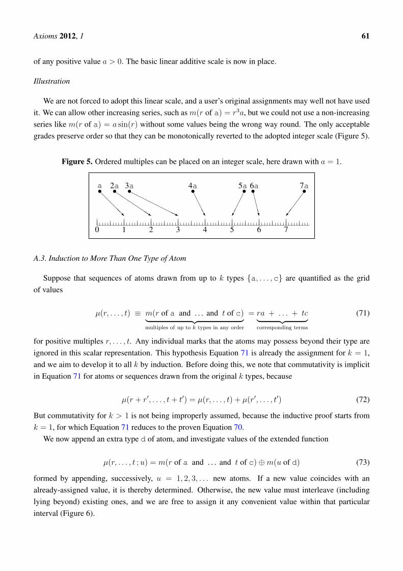
We are not forced to adopt this linear scale, and a user’s original assignments may well not have usedit. We can allow other increasing series, such as m(r of a) = r3a, but we could not use a non-increasingseries like m(r of a) = a sin(r) without some values being the wrong way round. The only acceptablegrades preserve order so that they can be monotonically reverted to the adopted integer scale (Figure 5).

Figure 5. Ordered multiples can be placed on an integer scale, here drawn with a = 1.

0 1

@@@@R

•a

2

QQQQQQs

•2a

3

HHHHHH

HHj

•3a

4

AAAAU

•4a

5

�����

•5a

6

CCCCW

•6a

7

����/

•7a

A.3. Induction to More Than One Type of Atom

Suppose that sequences of atoms drawn from up to k types {a, . . . ,c} are quantified as the gridof values

µ(r, . . . , t) ≡ m(r of a and . . . and t of c)︸ ︷︷ ︸multiples of up to k types in any order

= ra + . . . + tc︸ ︷︷ ︸corresponding terms

(71)

for positive multiples r, . . . , t. Any individual marks that the atoms may possess beyond their type areignored in this scalar representation. This hypothesis Equation 71 is already the assignment for k = 1,and we aim to develop it to all k by induction. Before doing this, we note that commutativity is implicitin Equation 71 for atoms or sequences drawn from the original k types, because

µ(r + r′, . . . , t+ t′) = µ(r, . . . , t) + µ(r′, . . . , t′) (72)

But commutativity for k > 1 is not being improperly assumed, because the inductive proof starts fromk = 1, for which Equation 71 reduces to the proven Equation 70.

We now append an extra type d of atom, and investigate values of the extended function

µ(r, . . . , t ;u) = m(r of a and . . . and t of c)⊕m(u of d) (73)

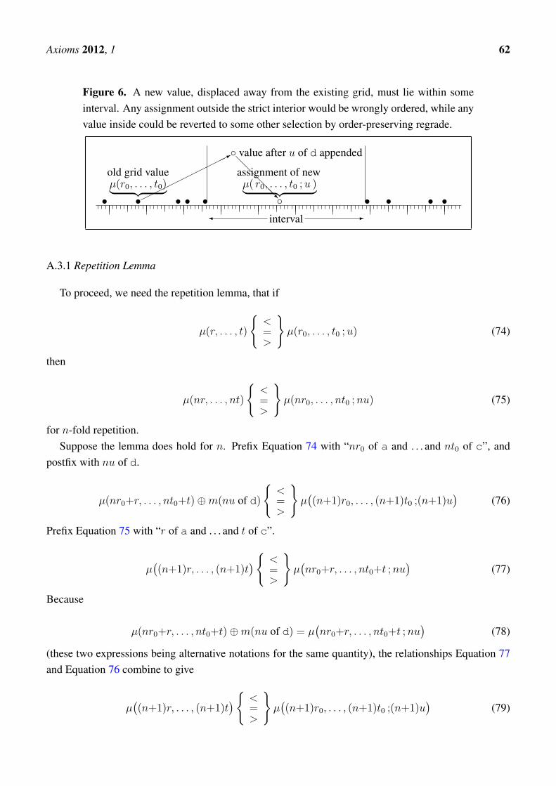
formed by appending, successively, u = 1, 2, 3, . . . new atoms. If a new value coincides with analready-assigned value, it is thereby determined. Otherwise, the new value must interleave (includinglying beyond) existing ones, and we are free to assign it any convenient value within that particularinterval (Figure 6).

Axioms 2012, 1 62

Figure 6. A new value, displaced away from the existing grid, must lie within someinterval. Any assignment outside the strict interior would be wrongly ordered, while anyvalue inside could be reverted to some other selection by order-preserving regrade.

• •����

���

���*

• • •� interval -

◦ • • • •

◦ value after u of d appended@@@@@R

old grid valueµ(r0, . . . , t0)︸ ︷︷ ︸ assignment of new

µ( r0, . . . , t0 ;u )︸ ︷︷ ︸

A.3.1 Repetition Lemma

To proceed, we need the repetition lemma, that if

µ(r, . . . , t)

{<=>

}µ(r0, . . . , t0 ;u) (74)

then

µ(nr, . . . , nt)

{<=>

}µ(nr0, . . . , nt0 ;nu) (75)

for n-fold repetition.Suppose the lemma does hold for n. Prefix Equation 74 with “nr0 of a and . . . and nt0 of c”, and

postfix with nu of d.

µ(nr0+r, . . . , nt0+t)⊕m(nu of d)

{<=>

}µ((n+1)r0, . . . , (n+1)t0 ;(n+1)u

)(76)

Prefix Equation 75 with “r of a and . . . and t of c”.

µ((n+1)r, . . . , (n+1)t

){ <=>

}µ(nr0+r, . . . , nt0+t ;nu

)(77)

Because

µ(nr0+r, . . . , nt0+t)⊕m(nu of d) = µ(nr0+r, . . . , nt0+t ;nu

)(78)

(these two expressions being alternative notations for the same quantity), the relationships Equation 77and Equation 76 combine to give

µ((n+1)r, . . . , (n+1)t

){ <=>

}µ((n+1)r0, . . . , (n+1)t0 ;(n+1)u

)(79)

Axioms 2012, 1 63

So, if Equation 75 holds for n, it also holds for n + 1. It does hold for n = 1, proving by induction therepetition lemma for all n = 1, 2, 3, . . . .

A.3.2 Separation

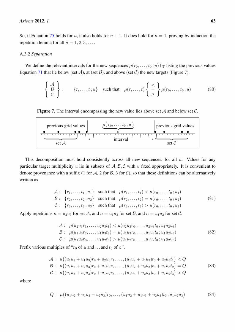
We define the relevant intervals for the new sequences µ(r0, . . . , t0 ;u) by listing the previous valuesEquation 71 that lie below (set A), at (set B), and above (set C) the new targets (Figure 7). ABC

: {r, . . . , t ;u} such that µ(r, . . . , t)

{<=>

}µ(r0, . . . , t0 ;u) (80)

Figure 7. The interval encompassing the new value lies above set A and below set C.

• • • • •� interval -

◦ • • • •previous grid values previous grid valuesµ( r0, . . . , t0 ;u )︸ ︷︷ ︸︸ ︷︷ ︸

set A︸ ︷︷ ︸

set C

This decomposition must hold consistently across all new sequences, for all u. Values for anyparticular target multiplicity u lie in subsets of A,B, C with u fixed appropriately. It is convenient todenote provenance with a suffix (1 for A, 2 for B, 3 for C), so that these definitions can be alternativelywritten as

A : {r1, . . . , t1 ;u1} such that µ(r1, . . . , t1) < µ(r0, . . . , t0 ;u1)

B : {r2, . . . , t2 ;u2} such that µ(r2, . . . , t2) = µ(r0, . . . , t0 ;u2)

C : {r3, . . . , t3 ;u3} such that µ(r3, . . . , t3) > µ(r0, . . . , t0 ;u3)

(81)

Apply repetitions n = u2u3 for set A, and n = u1u3 for set B, and n = u1u2 for set C.

A : µ(u2u3r1, . . . , u2u3t1) < µ(u2u3r0, . . . , u2u3t0 ;u1u2u3)

B : µ(u1u3r2, . . . , u1u3t2) = µ(u1u3r0, . . . , u1u3t0 ;u1u2u3)

C : µ(u1u2r3, . . . , u1u2t3) > µ(u1u2r0, . . . , u1u2t0 ;u1u2u3)

(82)

Prefix various multiples of “r0 of a and . . . and t0 of c”.

A : µ((u1u2 + u1u3)r0 + u2u3r1, . . . , (u1u2 + u1u3)t0 + u2u3t1

)< Q

B : µ((u1u2 + u2u3)r0 + u1u3r2, . . . , (u1u2 + u2u3)t0 + u1u3t2

)= Q

C : µ((u1u3 + u2u3)r0 + u1u2r3, . . . , (u1u3 + u2u3)t0 + u1u2t3

)> Q

(83)

where

Q = µ((u1u2 + u1u3 + u2u3)r0, . . . , (u1u2 + u1u3 + u2u3)t0 ;u1u2u3

)(84)

Axioms 2012, 1 64

Evaluate the left-hand sides and eliminate the common right-hand sides Q.((u1u2 + u1u3)r0 + u2u3r1

)a+ · · ·+

((u1u2 + u1u3)t0 + u2u3t1

)c

<((u1u2 + u2u3)r0 + u1u3r2

)a+ · · ·+

((u1u2 + u2u3)t0 + u1u3t2

)c

<((u1u3 + u2u3)r0 + u1u2r3

)a+ · · ·+

((u1u3 + u2u3)t0 + u1u2t3

)c

(85)

Subtract (u1u2 + u1u3 + u2u3)(r0a+ · · ·+ t0c) and divide by u1u2u3.((r1 − r0)a+ · · ·+ (t1 − t0)c

)/ u1︸ ︷︷ ︸

any member of A

<((r2 − r0)a+ · · ·+ (t2 − t0)c

)/ u2︸ ︷︷ ︸

any member of B

<((r3 − r0)a+ · · ·+ (t3 − t0)c

)/ u3︸ ︷︷ ︸

any member of C

(86)

Taking ((r − r0)a+ · · ·+ (t− t0)c) / u as the statistic, all members of A lie beneath all members ofB, which in turn lie beneath all members of C. We can now assign the value of µ(r0, . . . , t0 ;u) for sometarget multiple u. The treatment differs somewhat according to whether or not B is empty.

A.3.3 Assignment When B Has Members

If B is non-empty, we now show that all its members share a common value. Let two members be{r, . . . , t ;u} and {r′, . . . , t′ ;u′} (the suffix “2” is temporarily redundant), so that, by definition,

µ(r, . . . , t) = µ(r0, . . . , t0 ;u)

µ(r′, . . . , t′) = µ(r0, . . . , t0 ;u′)(87)

Apply repetitions by u′ and u, respectively.

µ(u′r, . . . , u′t) = µ(u′r0, . . . , u′t0 ;uu′)

µ(ur′, . . . , ut′) = µ(ur0, . . . , ut0 ;uu′)(88)

Prefix multiples u and u′ of “r0 of a and . . . and t0 of c”.

µ(ur0 + u′r, . . . , ut0 + u′t) = µ(ur0 + u′r0, . . . , ut0 + u′t0 ;uu′)

µ(u′r0 + ur′, . . . , u′t0 + ut′) = µ(ur0 + u′r0, . . . , ut0 + u′t0 ;uu′)(89)

Evaluate the left-hand sides and eliminate the common right-hand side.

(ur0 + u′r)a+ · · ·+ (ut0 + u′t)c = (u′r0 + ur′)a+ · · ·+ (u′t0 + ut′)c (90)

Subtract (u+ u′)(r0a+ · · ·+ t0c) and divide by uu′,

(r − r0)a+ · · ·+ (t− t0)cu

=(r′ − r0)a+ · · ·+ (t′ − t0)c

u′= d (91)

in which d denotes this common value now seen to be shared by all members of B. Using the definitionsagain, evaluating, and using this common value gives

µ(r0, . . . , t0 ;u) = µ(r, . . . , t) = ra+ · · ·+ tc = r0a+ · · ·+ t0c+ ud (92)

Axioms 2012, 1 65

where d is seen to be the value m(d) of a single atom of type d. By Equation 91, this value is rationallyrelated to the previous values a, . . . , c.

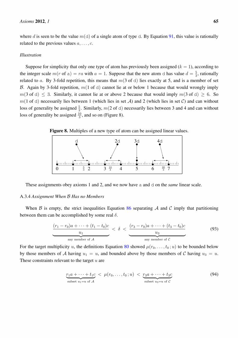
Illustration

Suppose for simplicity that only one type of atom has previously been assigned (k = 1), according tothe integer scale m(r of a) = ra with a = 1. Suppose that the new atom d has value d = 5

3, rationally

related to a. By 3-fold repetition, this means that m(3 of d) lies exactly at 5, and is a member of setB. Again by 3-fold repetition, m(1 of d) cannot lie at or below 1 because that would wrongly implym(3 of d) ≤ 3. Similarly, it cannot lie at or above 2 because that would imply m(3 of d) ≥ 6. Som(1 of d) necessarily lies between 1 (which lies in set A) and 2 (which lies in set C) and can withoutloss of generality be assigned 5

3. Similarly, m(2 of d) necessarily lies between 3 and 4 and can without

loss of generality be assigned 103

, and so on (Figure 8).

Figure 8. Multiples of a new type of atom can be assigned linear values.

0 1 2 3 4 5 6 7• • • • • • • •

AAAAU

•d

53

�����

•2d

103

?

•3dCCCCW

•4d

203

� - � - • � -

These assignments obey axioms 1 and 2, and we now have a and d on the same linear scale.

A.3.4 Assignment When B Has no Members

When B is empty, the strict inequalities Equation 86 separating A and C imply that partitioningbetween them can be accomplished by some real δ.

(r1 − r0)a+ · · ·+ (t1 − t0)cu1︸ ︷︷ ︸

any member of A

< δ <(r3 − r0)a+ · · ·+ (t3 − t0)c

u3︸ ︷︷ ︸any member of C

(93)

For the target multiplicity u, the definitions Equation 80 showed µ(r0, . . . , t0 ;u) to be bounded belowby those members of A having u1 = u, and bounded above by those members of C having u3 = u.These constraints relevant to the target u are

r1a+ · · ·+ t1c︸ ︷︷ ︸subset u1=u of A

< µ(r0, . . . , t0 ;u) < r3a+ · · ·+ t3c︸ ︷︷ ︸subset u3=u of C

(94)

Axioms 2012, 1 66

which is equivalent to

(r1 − r0)a+ · · ·+ (t1 − t0)cu︸ ︷︷ ︸

subset u1=u of A

<µ(r0, . . . , t0 ;u)− (r0a+ · · ·+ t0c)

u

<(r3 − r0)a+ · · ·+ (t3 − t0)c

u︸ ︷︷ ︸subset u3=u of C

(95)

Because this refers to subsets involving a single u rather than the entire sets involving all u, it is a weakerconstraint than the preceding global constraint Equation 93 was on δ. In other words, its central quantity(µ(r0, . . . , t0 ;u)− (r0a+ · · ·+ t0c)

)/ u is allowed to lie anywhere within an interval that contains the

narrower interval containing δ. Accordingly, it is legitimate to assign

µ(r0, . . . , t0 ;u)− (r0a+ · · ·+ t0c)

u= δ (96)

which automatically satisfies all the relevant constraints Equation 95. So the simple assignment

µ(r0, . . . , t0 ;u) = r0a+ · · ·+ t0c+ uδ (97)

automatically falls in the correct interval. The only freedom is regrade to some alternative value withinthe relevant interval.

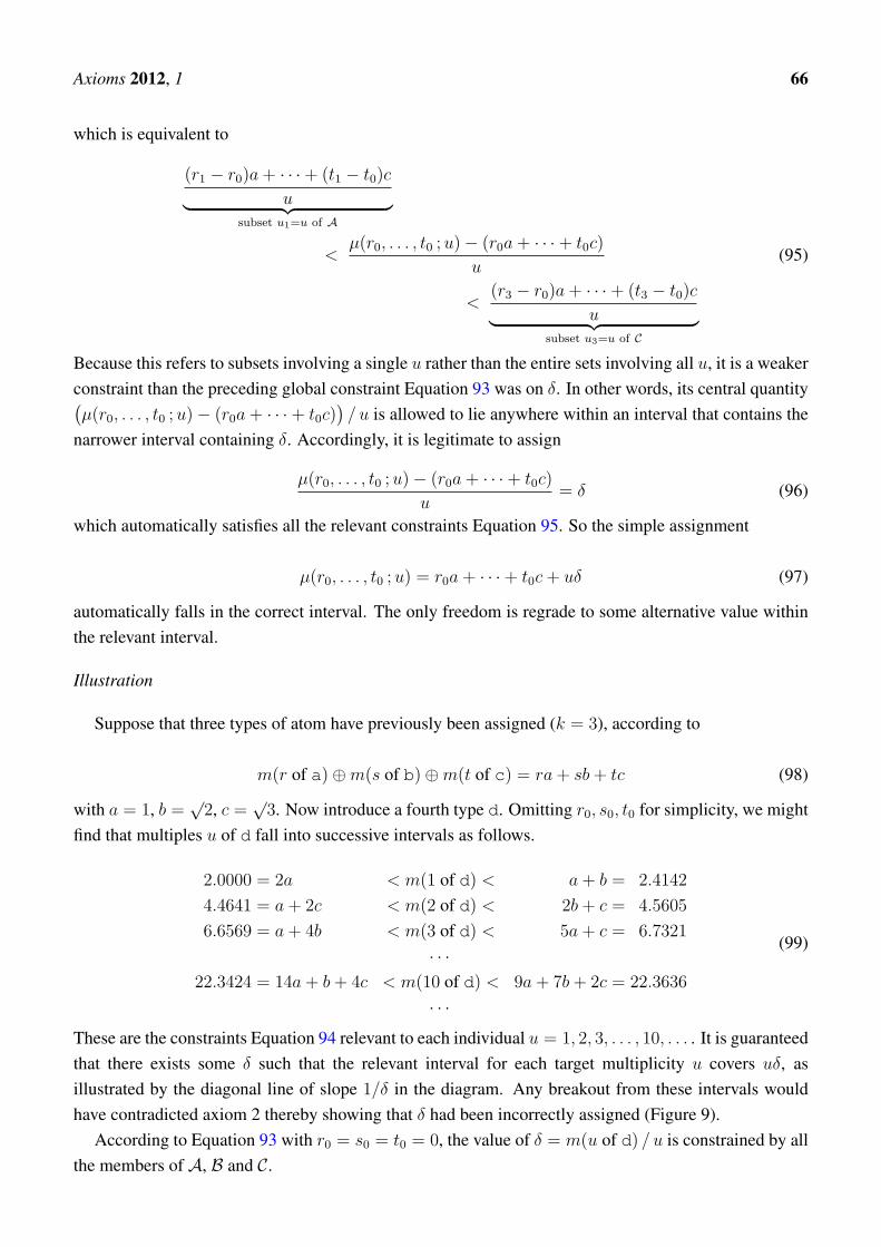
Illustration

Suppose that three types of atom have previously been assigned (k = 3), according to

m(r of a)⊕m(s of b)⊕m(t of c) = ra+ sb+ tc (98)

with a = 1, b =√

2, c =√

3. Now introduce a fourth type d. Omitting r0, s0, t0 for simplicity, we mightfind that multiples u of d fall into successive intervals as follows.

2.0000 = 2a < m(1 of d) < a+ b = 2.4142

4.4641 = a+ 2c < m(2 of d) < 2b+ c = 4.5605

6.6569 = a+ 4b < m(3 of d) < 5a+ c = 6.7321

· · ·22.3424 = 14a+ b+ 4c < m(10 of d) < 9a+ 7b+ 2c = 22.3636

· · ·

(99)

These are the constraints Equation 94 relevant to each individual u = 1, 2, 3, . . . , 10, . . . . It is guaranteedthat there exists some δ such that the relevant interval for each target multiplicity u covers uδ, asillustrated by the diagonal line of slope 1/δ in the diagram. Any breakout from these intervals wouldhave contradicted axiom 2 thereby showing that δ had been incorrectly assigned (Figure 9).

According to Equation 93 with r0 = s0 = t0 = 0, the value of δ = m(u of d) / u is constrained by allthe members of A, B and C.

Axioms 2012, 1 67

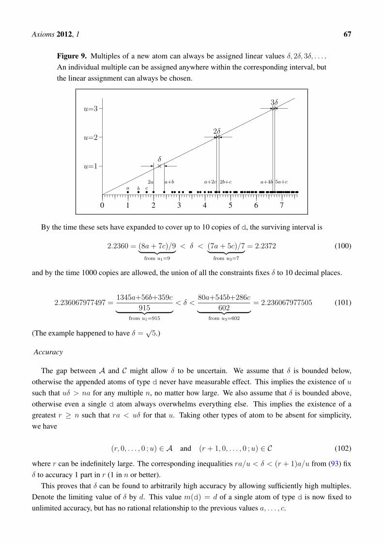
Figure 9. Multiples of a new atom can always be assigned linear values δ, 2δ, 3δ, . . . .An individual multiple can be assigned anywhere within the corresponding interval, butthe linear assignment can always be chosen.

0 1 2 3 4 5 6 7

•a•b •

c• • •• • • •• •• • •• ••• •••• ••• ••••••••• •••••••••••••••••••••••••��

���

���

���

���

���

���

���

���

���

�

u=1

u=2

u=3

-

2a

�

a+b

-

a+2c

�

2b+c

-

a+4b

�

5a+c

×δ

×2δ

×3δ

By the time these sets have expanded to cover up to 10 copies of d, the surviving interval is

2.2360 = (8a+ 7c)/9︸ ︷︷ ︸from u1=9

< δ < (7a+ 5c)/7︸ ︷︷ ︸from u3=7

= 2.2372 (100)

and by the time 1000 copies are allowed, the union of all the constraints fixes δ to 10 decimal places.

2.236067977497 =1345a+56b+359c

915︸ ︷︷ ︸from u1=915

< δ <80a+545b+286c

602︸ ︷︷ ︸from u3=602

= 2.236067977505 (101)

(The example happened to have δ =√

5.)

Accuracy

The gap between A and C might allow δ to be uncertain. We assume that δ is bounded below,otherwise the appended atoms of type d never have measurable effect. This implies the existence of usuch that uδ > na for any multiple n, no matter how large. We also assume that δ is bounded above,otherwise even a single d atom always overwhelms everything else. This implies the existence of agreatest r ≥ n such that ra < uδ for that u. Taking other types of atom to be absent for simplicity,we have

(r, 0, . . . , 0 ;u) ∈ A and (r + 1, 0, . . . , 0 ;u) ∈ C (102)

where r can be indefinitely large. The corresponding inequalities ra/u < δ < (r + 1)a/u from (93) fixδ to accuracy 1 part in r (1 in n or better).

This proves that δ can be found to arbitrarily high accuracy by allowing sufficiently high multiples.Denote the limiting value of δ by d. This value m(d) = d of a single atom of type d is now fixed tounlimited accuracy, but has no rational relationship to the previous values a, . . . , c.

Axioms 2012, 1 68

A.3.5 End of Inductive Proof

Whether or not B had members, the assignment

µ(r0, . . . , t0 ;u) = r0a+ · · ·+ t0c+ ud (103)

obeys all the defining inequalities Equation 80. This updates the original assignment Equation 71 fromk atom types to k + 1, so by induction from k = 1 it holds for any k.

m(r of a and . . . and t of c and . . . and v of e)︸ ︷︷ ︸any number of types in any order

= ra+ · · ·+ tc+ · · ·+ ve︸ ︷︷ ︸corresponding terms

(104)

Atom types in the above expression are often different, but do not need to be, and the formularepresents the quantification of a general sequence. Embedded in it, and equivalent to it, is the sumrule x⊕ y = x+ y for the values m(x) = x and m(y) = y of arbitrary sequences. Any order-preservingregrade Θ is also permitted, but no order-breaking transform is permitted.

This completes the inductive proof for atoms of positive style. The proof holds equally well foratoms of negative style, for which the values are negative. Meanwhile, Equation 68 shows that atomsof null style have zero value. So, even if the atoms may have arbitrary style, Equation 104 offers theonly consistent combination rule. The result thus holds for atom values of arbitrary sign and arbitrarymagnitude, though the nature of the constructive proof requires atom multiplicities to be non-negative.ut

A.4. Axioms are Minimal

Theorem:

Axioms 1a, 1b, 2 are individually required.

Proof:

We construct operators© (“not quite⊕”) which deny each axiom in turn, while not being a monotonicstrictly increasing regrade of addition.

Without axiom 1a (postfix ordering), the definition

a© b = bac+ b (105)

where bac is the integer at or immediately below a, satisfies axioms 1b and 2 but cannot be equivalent toaddition because it is not commutative; a© b 6= b© a. So axiom 1a is required.

Without axiom 1b (prefix ordering), the definition

a© b = a+ bbc (106)

satisfies axioms 1a and 2, but cannot be equivalent to addition because it is not commutative. So axiom 1bis required.

Axioms 2012, 1 69

Without axiom 2 (associativity), the definition

x© y = x2 + y2 (107)

satisfies axioms 1a and 1b (ordering), and also happens to be continuous and commutative(x© y = y©x). Yet it cannot be equivalent to addition because Θ(x© y) = Θ(x) + Θ(y) has nosolution that would enable a regrade Θ. That can be shown by appropriately differencing δxδy to reachΘ(z+ ε)−2Θ(z)+Θ(z− ε) = 0 whose solution Θ(z) = Az+B fails to satisfy the supposedly definingEquation 107. Hence ordering is insufficient even when accompanied by continuity and commutativity.Axiom 2 (associativity) is definitely required. ut

B. Appendix B: Product Theorem

Theorem:The solution of the functional product Equation

Ψ(τ + ξ) + Ψ(τ + η) = Ψ(τ + ζ(ξ, η)

)(108)

in which τ , ξ and η are independent real variables and Ψ is positive is

Ψ(x) = CeAx (109)

where A and C are constants (C necessarily being positive).

B.1. Proof:

The quoted solution is easily seen to satisfy the product equation, which demonstrates existence. Theremaining question is whether the solution is unique.

First, we take the special case ξ = η, so that ζ − ξ and ζ − η take a common value a. This gives a2-term recurrence

2Ψ(τ + ζ − a) = Ψ(τ + ζ) (110)

in which τ and ζ remain independent, though a might be constant. In fact, a must be constant, otherwisethere would be no solution for Ψ. Consequently, Ψ behaves geometrically with

Ψ(θ + na) = 2nΨ(θ) (111)

for any integer n, θ being arbitrary. Although this plausibly suggests that Ψ will be exponential, that isnot yet proved because Ψ could still be arbitrary within any assignment range of width a.

To complete the proof, take a second special case where ζ − ξ and (ζ − η) / 2 take a common valueb. This gives a 3-term recurrence

Ψ(τ + ζ − b) + Ψ(τ + ζ − 2b) = Ψ(τ + ζ) (112)

Axioms 2012, 1 70

in which τ and ζ remain independent, though b might be constant. In fact, b must be constant, otherwisethere would be no solution for Ψ. The solution is

Ψ(θ +mb) =

(2 Ψ(θ)

5+√

5+

Ψ(θ+b)√5

)(1+√

5

2

)m+

(2 Ψ(θ)

5−√

5− Ψ(θ+b)√

5

)(−2

1+√

5

)m(113)

for any integer m, θ being arbitrary.This combines with the 2-term formula to make

Ψ(θ +mb− na) =

(2 Ψ(θ)

5+√

5+

Ψ(θ+b)√5

)em log

(1+√

52

)−n log 2 +

(−1)m(

2 Ψ(θ)

5−√

5− Ψ(θ+b)√

5

)e−m log

(1+√

52

)−n log 2

(114)

For any integer n, there is an even integer m for which 0 ≤ mb − na < 2b so that all three argumentsof Ψ lie in the range [θ, θ + 2b]. As n is allowed to increase indefinitely, so does this m in proportionm/n ≈ a/b. Depending on the sign of n, at least one of the exponents ±m log 1+

√5

2− n log 2 can

become indefinitely large and positive. Unbounded values of Ψ being unacceptable, the coefficient ofthat exponent must vanish. So either

Ψ(θ +mb− na) = Ψ(θ) em log(1+

√5

2

)−n log 2 (115)

(first term only) or

Ψ(θ +mb− na) = (−1)mΨ(θ) e−m log(1+

√5

2

)−n log 2 (116)

(second term only, and even m makes the sign (−1)m = 1). In the first case, bounded Ψ requires

b

a=

log(1+

√5

2

)log 2

(117)

and in the second case, bounded Ψ requires

b

a= −

log(1+

√5

2

)log 2

(118)

Either way,

Ψ(θ +mb− na) = Ψ(θ) eA(mb−na) (119)

with A constant.Although this strongly suggests that Ψ will be exponential, that is not yet fully proved because offsets

mb − na with even m are only a subset of the reals. There could be one scaling for arguments θ of theform mb−na, another for the form

√2 +mb−na, yet another for π+mb−na, and so on. Fortunately,

b/a is irrational, so the offset mb − na can approach any real value x arbitrarily closely. Express x asx = mb− na+ ε with m and n chosen to make ε arbitrarily small. Then

Ψ(x) = eA(mb−na)Ψ(ε) = eA(x−ε)Ψ(ε) ≈ eAxΨ(ε) (120)

Axioms 2012, 1 71

because eAε ≈ 1. Separating variables, Ψ(ε) ≈ constant, giving

(solution) Ψ(x) = CeAx (121)

to arbitrarily high precision (ε→ 0) with constant C.This obeys the original product equation without further restriction and is the general solution, with

corollary eAξ + eAη = eAζ defining ζ(ξ, η) and confirming that a = A−1 log 2 and b = A−1 log(1+√

52

)

were appropriate constants. ut

The sought inverse, in terms of the constants A and C, is

(inverse) Θ(u) =1

Alog

u

C (122)

in which u and hence C are both positive.

C. Appendix C: Variational Theorem

Theorem:The solution of the functional variational equation

H ′(mxmy) = λ(mx) + µ(my) (123)

with positive mx and my is

H(m) = A+Bm+ C(m logm−m) (124)

where A, B, C are constants.

C.1. Proof:

The quoted solution is easily seen to satisfy the variational equation, with corollaries that the functionsλ and µ are logarithmic, which demonstrates existence. The remaining question is whether the solutionis unique.

Write logmx = u, logmy = v, and rewrite the functions as λ∗(u), µ∗(v) and H ′(m) = h(logm).

h(u+ v) = λ∗(u) + µ∗(v) (125)

Put v = 0 to get λ∗(u) = h(u)− constant and u = 0 to get µ∗(v) = h(v)− constant.

h(u+ v) = h(u) + h(v)−B (126)

This is Cauchy’s functional equation ([14])

f(u+ v) = f(u) + f(v) (127)

Axioms 2012, 1 72

for f(t) = h(t)−B from which f(nt) = nf(t) and then f( rnt) = r

nf(t) follow by induction for integer

r and n. Hence

f(t) = ct (128)

where c = f(t0) / t0 evaluated at any convenient base t0. Awkwardly, the recurrence only relates toa rational grid—there could be one value of c for rational multiples of 1, another value for rationalmultiples of

√2, yet another for rational multiples of π, and so on. Fortunately, the sought function H is

an integral of f , on which such infinitesimal detail has no effect.To show that, we blur functions φ(u, v) by convolving them with the following unit-mass ellipse,

chosen to blur u, v and u+v equally, according to

Φ(u, v) =

∫∫dx dy

1(x2 + xy + y2 < 34ε2)

√3πε2/2

φ(u− x, v − y) (129)

For small width ε, blurring has negligible macroscopic effect. The convolution transforms the Cauchyequation to the same form

F (u+ v) = F (u) + F (v) (130)

as before, with the new function

F (t) =

∫ ε

−εdx

2√ε2 − x2

πε2f(t− x) (131)

being a continuous version of the original f , narrowly blurred over finite support. With continuity inplace, the Cauchy solution

F (t) = Ct (132)

can only have one value for the constant C.Finally, the definition dH/dm = h(logm) = B + f(logm) yields

H(m) = Bm+

∫ m

f(logm′)dm′ (integrate)

= Bm+

∫ logm

f(t) etdt (change variable)

= Bm+

∫ ε

−εdx

2√ε2 − x2

πε2

∫ logm

f(t) etdt (insert blurring)

= Bm+

∫ ε

−εdx

2√ε2 − x2

πε2

∫ x+logm

f(t− x) et−xdt (offset dummy t)

≈ Bm+

∫ ε

−εdx

2√ε2 − x2

πε2

∫ logm

f(t− x) etdt (|x| ≤ ε small) !

= Bm+

∫ logm

F (t) etdt (definition of F )

= Bm+ C

∫ logm

tetdt (substitute)

(133)

Axioms 2012, 1 73

Hence, to arbitrarily high precision (ε→ 0), H integrates to

H(m) = A+Bm+ C(m logm−m) . (134)

This obeys the original variational equation with corollaries λ(x) = B1 + C log(x) and µ(x) =

B2 + C log(x) where B1 +B2 = B, and is the general solution. ut

c© 2012 by the authors; licensee MDPI, Basel, Switzerland. This article is an open access articledistributed under the terms and conditions of the Creative Commons Attribution license(http://creativecommons.org/licenses/by/3.0/).