OPEN ACCESS atmosphere - Semantic Scholar · PDF fileOPEN ACCESS atmosphere ... 22010...

Atmosphere 2015, 6, 579-606; doi:10.3390/atmos6050579OPEN ACCESS

atmosphereISSN 2073-4433

www.mdpi.com/journal/atmosphere

Article

Storm Identification, Tracking and Forecasting UsingHigh-Resolution Images of Short-Range X-Band RadarSajid Shah 1,2,*, Riccardo Notarpietro 1 and Marco Branca 1

1 DET, Politecnico di Torino, Corso Duca degli Abruzzi, 10129 Turin, Italy;E-Mails: [email protected] (R.N.); [email protected] (M.B.)

2 Computer Science Department, COMSATS Institute of Information Technology,22010 Abbottabad, Pakistan

* Author to whom correspondence should be addressed; E-Mail: [email protected];Tel.: +39-011-090-4623.

Academic Editors: Richard Müller and Guifu Zhang

Received: 27 November 2014 / Accepted: 17 April 2015 / Published: 6 May 2015

Abstract: Rain nowcasting is an essential part of weather monitoring. It plays a vitalrole in human life, ranging from advanced warning systems to scheduling open air eventsand tourism. A nowcasting system can be divided into three fundamental steps, i.e.,storm identification, tracking and nowcasting. The main contribution of this work is topropose procedures for each step of the rain nowcasting tool and to objectively evaluatethe performances of every step, focusing on two-dimension data collected from short-rangeX-band radars installed in different parts of Italy. This work presents the solutionof previously unsolved problems in storm identification: first, the selection of suitablethresholds for storm identification; second, the isolation of false merger (loosely-connectedstorms); and third, the identification of a high reflectivity sub-storm within a large storm.The storm tracking step of the existing tools, such as TITANand SCIT, use only up totwo storm attributes, i.e., center of mass and area. It is possible to use more attributesfor tracking. Furthermore, the contribution of each attribute in storm tracking is yet to beinvestigated. This paper presents a novel procedure called SALdEdA (structure, amplitude,location, eccentricity difference and areal difference) for storm tracking. This work alsopresents the contribution of each component of SALdEdA in storm tracking. The secondorder exponential smoothing strategy is used for storm nowcasting, where the growth anddecay of each variable of interest is considered to be linear. We evaluated the major steps ofour method. The adopted techniques for automatic threshold calculation are assessed with

Atmosphere 2015, 6 580

a 97% goodness. False merger and sub-storms within a cluster of storms are successfullyhandled. Furthermore, the storm tracking procedure produced good results with an accuracyof 99.34% for convective events and 100% for stratiform events.

Keywords: storm identification; storm tracking; nowcasting; forecasting; thresholding;image segmentation

1. Introduction

Normally, long-range radars are used for weather monitoring, but these radars are power demanding,costly in terms of price and are not suitable for narrow valleys surrounded by high mountains,while X-band radars are quite efficient for monitoring localized rain fall events with small basins ofinterest. X-band radars provide high spatial and temporal resolution, which is required for hydrologicalapplications in urban areas [1]. Data for experiments are collected from MicroRadarNetr (see [2,3])designed by the Remote Sensing Group of the Polytechnic of Turin, Italy. It is a network of low-cost,low-power consumption, unmanned, X-band, micro-radars. Radar echoes are quantized into imagerydata using eight-bit radiometric resolution resulting in a grey scale image with 1024 × 1024 imagedimensions. Real-time precipitation observations are available at (http://meteoradar.polito.it).

In this paper, we present new methods for the three major steps of rain nowcasting: stormidentification, tracking and forecasting. All steps are objectively evaluated.

A storm can be defined as an object composed of connected pixels in a radar image where thereflectivity of all pixels is greater than a reflectivity threshold (Tz) and the area of this object is greaterthan an areal threshold (Ta) [4]. Storm identification is comprised of identifying a storm’s boundaries,calculating its area, centroid, mean and maximum reflectivity where the centroid is the center ofmass of the storm. Storm identification starts with segmenting the image into meaningful sub-regions(objects/storms) on the basis of some properties, such as intensities (grey levels/reflectivity), color andtexture. Many storm identification techniques, like [4–8], are based on global thresholding. We havealso adopted this procedure. Global thresholding can be categorized as single- and multi-level, as wellas manual, semi-automated and automated. In the manual one, the user has to set the threshold valueby trial and error, while in the semi-automated one, the user has to enter an initial value, and the systemcomputes the rest of the value(s). A fully-automated system does not need user intervention and choosesthe thresholds automatically.

The single threshold systems face three major problems. The first one is choosing a suitable thresholdvalue. If the initial threshold value is too high, storm(s) initiation may not be detected; also, stratiformevents may be ignored, and setting it to a low value may result in an unrealistically large storm. Thesecond problem is the weak connection between two or more storms, called false merger, while the thirdone is the inability of identifying sub-storms within a cluster of storms. In the case of false merger,the identification algorithm falsely treated these loosely connected storms as a single (merged) storm(see Figure 1). Clusters of storms can be defined as a large storm that has further strong reflectivitysub-storms (see Figure 2).


Figure 1. (a) False merger; (b) result of erosion.

Figure 2. (a) Cluster of storms; (b) hierarchical form of storms after applying different levelsof thresholds.

To overcome the problem of choosing a suitable initial threshold value, we have proposedfully-automated thresholding techniques (discussed in Sections 3.1.1 and 3.1.2) based on ThreshGW(G stands for Gonzalez and W for Woods) [9] and graythresh [10]. The false-merger problem is solvedby using mathematical morphology (given in Section 3.3), particularly morphological erosion, discussedin [9]. A multi-level thresholding technique, discussed in Section 3.4, is used to overcome the problem ofidentifying sub-storms within a cluster of storm(s). Unlike [8], we did not discard any identified storm;also, we did not iteratively dilate (expand) the identified storms to maintain the original structure, likein [6,7].

A track can be defined as the path followed by a storm during its complete life time or fromits initiation to the last time it was observed. The storm tracking can be defined as the timeassociation of storms identified at time instance t to the storms already identified and tracked attime instance t-1. Storm(s) splitting, merging, initiation and disappearance make tracking difficult.Storm tracking is discussed in detail in Section 4. Tracking algorithms can be divided into two maincategories, i.e., centroid based [4,5,8,11,12] and those which are based on cross-correlation [13–17].Both techniques have benefits and drawbacks. Centroid-based algorithms can track individual stormsmore adequately and can provide more information about individual storms. In these algorithms, thecenter of mass (centroid) of storms is used for tracking. Two storms in two consecutive time instancesnearest to each other are candidates for matching. Meanwhile, those algorithms that are based on thecross-correlation produce more accurate speed and direction information for large areas [8]. The hybridof these two categories was developed by [7,18].

Our proposed procedure is called the combinational optimization technique, because the centroid isused with additional storm attributes for tracking. The centroid-based algorithms proposed until now donot use the reflectivity/precipitation distribution of storms for tracking. In our structure, the amplitude,


location, eccentricity difference and areal difference (SALdEdA) variables, we have used the reflectivityand shape information of a storm for tracking. The basic idea behind mapping (associating) two objectsof two consecutive time instances is to find how similar they are in structure, amplitude, circularityand area and how closely these storms are located. A global cost function (presented in Section 4.2) isformulated. At this stage, the problem of associating two storms becomes a combinatorial optimizationproblem. The aim is to find a matching where the global cost function is minimized. Hungarian (see [19])is the candidate algorithm for solving our problem, because it is relatively easy to implement.

Section 5 discusses storm forecasting. Forecasting is the prediction of future event(s). Our variablesof interest for forecasting are the area of the storm, the major/minor axis length, the angle of orientation,the speed and the direction. We have adopted first and second order exponential smoothing strategies inorder to model our variables of interest.

2. State-of-the-Art

As mentioned before, most of the early attempts for storm identification were threshold based.A few examples are discussed in this section.

The original TITAN, discussed in [4], uses a single reflectivity threshold to identify the storm(s).The updated version of TITAN uses two reflectivity thresholds to overcome the problem of false-mergers.TITAN defines storms as a contiguous region exceeding thresholds for both reflectivity and volume.The identification procedure consists of two steps: first, the identification of contiguous sequences ofpoints (called run) for which the reflectivity exceeds Tz (minimum threshold value in dBZ); second, thegrouping of all runs that are adjacent. Storms with volumes less than volumetric threshold Tv aredropped. TITAN calculates storm properties, such as centroid, vertically-integrated liquid (VIL),volume, etc. TITAN is unable to identify storm cells within a cluster of storms. Beside this, ifthe reflectivity threshold is kept high, TITAN is not capable of identifying storm initiation and alsostratiform events.

SCIT (the storm cell identification and tracking algorithm) is another algorithm that processesvolumetric reflectivity information by using a multi-level thresholding technique [8]. SCIT uses apredefined list of seven different reflectivity thresholds, i.e., 60, 55, 50, 45, 40, 35 and 30 dBZ.Identification of storms is carried out in different stages, starting from 1D (one-dimensional) dataprocessing, called a run, similar to TITAN. All runs are then combined into 2D storm components.Though SCIT has the strength to identify the storm cells within a cluster of storms, yet is unable todetect storm initiation or storms with a reflectivity less than 30 dBZ, consequently, it drops the stormsidentified by lower threshold values, which may be interesting for some users. Both TITAN and SCITface the problem of false merger isolation.

ETITAN (enhanced TITAN) was developed by [7]. The storm identification step is based on TITANand SCIT with some additional features. Identification of the run and grouping the adjacent runs issimilar to TITAN. ETITAN has the capability to identify sub-storms within a cluster of storms usingthe seven reflectivity thresholds as used by SCIT. In order to cope with the problem of false mergers,ETITAN has introduced mathematical morphology. SCIT dilates (expands) storms iteratively to maintain


the internal storm’s structure. ETITAN has a similar built-in problem as SCIT, such as its inability todetect storm(s) initiation or storms with lower reflectivity.

As mentioned earlier, storm tracking algorithms are mainly classified into two classes, i.e., centroidbased [4,5,8,11,12] and correlation based [13–17] algorithms. These approaches have been reviewedin [20], while [21] discusses the comparison of nine nowcasting tools deployed during the OlympicGames 2000, Sydney, Australia, under the umbrella of WWRP (World Weather Research Programme).

TITAN tracks the storms using a combinatorial optimization procedure [4]. A cost is calculated forevery pair of storms in t and t-1, which is the weighted sum of the distance between the centroids of thestorms and the difference in their volumes. A true set of tracks that minimizes the cost function is found.

The storm cell identification and tracking (SCIT) discussed by [8] identifies storm cells in twosuccessive radar scans and temporally associates the identified cells to find the track of every cell.The time difference between two consecutive radar scans is determined. If the time difference is greaterthan a certain time interval (20 min), discontinuity is recorded. Centroids of cells at time t-1 are projectedas a first estimate for the locations of cells in current time t-1 based on time instances t-k, where k > 1.Every cell of time t is associated with the closest cell in a searching radius. If there is no cell in thesearching circle, it is considered as a new cell.

The effective evaluation of tracking has not been explored very much by researchers.Johnson et al. [8] introduced a simple, but labor-intensive procedure for the tracking evaluation called“percentage correct”. It is simply the ratio of correctly-tracked storms and total tracks. Lakshmanan andSmith [22] proposed the following set of metrics based on statistics for each track:

1. Dur is the total life time (duration) of a track;2. The standard deviation of VIL (σv);3. The root mean square error of centroid positions from their optimal line fit.

The atmosphere cannot be predicted perfectly in a certain way, because of its non-linearity.According to Bellon et al. [23], the main reasons for the loss in forecast skill are not due to errorsin the forecast motion; rather, they are due to the unpredictable nature of the storms in terms of growthand decay. Therefore, statistical methods for forecasting are the essential part of forecasting tools [24].The most widely-used technique for weather forecasting is linear or least squares regression [24].Lu et al. [25] presented a weather predicting system based on a neural network and fuzzy inferencesystem, which is out of scope of the current work. TITAN assumes the decay and growth of stormsfollow a linear trend, while storm motion occurs along a straight line. A linear regression model, calleddouble exponential smoothing, is adopted for linear trend modeling of the variables of interest [4].

Forecast evaluation or validation and verification are the processes of assessing the quality offorecasts. Various kinds of forecasts validation techniques exist, where the basic criterion is to comparethe forecasts with the original observations. The definition of a good forecast is subjective, but generallyspeaking, a forecast is good if the difference between forecasts and the original observations is small.The famous technique for forecasts evaluation is the contingency table approach [26] used by [3,4,7].


3. Storm Identification

The storm/cell is the experimental unit and is respectively defined as a contiguous region withreflectivity and area above Tz and Ta. Storm identification is the recognition of individual storms’boundaries and computes their characteristics, i.e., centroids, area, major/minor radii and orientation, etc.Most of the storm-based weather forecasting systems use a thresholding technique for the identificationof storms/cells.

After identifying storm(s), we calculate the area of the storm(s) by counting the number of pixels inthe storm(s), and then, we apply the areal threshold value, i.e., Ta. The qualifying storm(s) is subjectedto further processing. Storms approximated by ellipses and attributes, like the centroid, major/minor axisorientation, etc., are calculated according to the procedure discussed in [27].

3.1. Thresholding

Single thresholding divides an image into two classes, i.e., background class (C0) and foregroundclass (C1). In the case of radar images, radar echoes are the foreground, while their absence isthe background of the image. Since we are interested in rain, pixels belonging to C0 are dropped,while pixels belonging to C1 are kept for further processing. A single threshold only separates thebackground from the foreground, but it is not capable of identifying different objects (storms/cells) inthe foreground. The foreground after applying a single threshold is called a cluster if it has sub-storms,as shown in Figure 2. To correctly separate the sub-storms of a cluster, multi-level thresholding, alsocalled multi-thresholding, is required. Most of the weather forecasting systems have left the choiceof selecting the initial threshold to the users of the system. Normally, the user performs some trialand error to choose the appropriate threshold. Our aim is to develop a fully-automated system capableof calculating a suitable initial threshold value and also to find out the number of appropriate levels.Many techniques have been developed for threshold calculation, such as histogram-, clustering- andentropy-based methods. Some of these techniques are parametrized and/or supervised, while others arenon-parametric and unsupervised methods. We have selected two methods, which are ThresholdGW [9]and graythresh [10], which are totally automated, non-parametric and unsupervised procedures. Thefirst method is not popular, but is easy to implement, while the second one is popular in the imageprocessing community. These methods calculate the initial threshold in the grey scale, which is thenconverted into radar reflectivities. Our system also supports single thresholding and semi-automaticmulti-level thresholding.

3.1.1. ThresholdGW

Gonzalez and Woods [9] describe an iterative procedure for automatic threshold selection. We namedit ThresholdGW. An initial estimate for Tz is calculated as the average of the maximum and minimumintensities in the radar image. The image is segmented into two classes, i.e., C0 and C1, using Tz. Themean Tz is calculated for each class, and the final Tz is the average of the mean of the backgroundand foreground.


3.1.2. Graythresh

The basic idea of graythresh is to divide image data into C0 and C1 on such a point that maximizesthe variance between the background and foreground classes, called between class variance σ2

B. Thehistogram of a gray scale image is computed where each bin corresponds to each gray level from zero to255. Each gray level is considered as a dividing point for which the between class variance is computed.Finally, a gray level with maximum σ2

B is selected as Tz. The detailed procedure is given in [10].

3.2. Storm Labeling

After applying thresholding, the next step is to group the qualifying pixels into different storms.The technique used for grouping together relevant pixels in different storms is called labeling. We startfrom the top left corner of the image and search for the first non-zero pixel, say p, at coordinate (x, y),and we label it as one. Now, the rest of the pixels can be connected to p by using two different adjacencycriteria [9]. A pixel p can have two horizontal and two vertical neighbors, according to the four-neighborsadjacency method, which can be represented by N4 (p), while p also has its four diagonal neighbors,which can be represented by ND (p). The union of N4 (p) and ND (p) results in the eight-neighborsadjacency method, which can be represented by N8 (p).

Pixels p and q are said to be four-adjacent if q is one and q ∈ N4 (p). Furthermore, p and q are said tobe eight-adjacent if q is one and q ∈ N8 (p). If p and q are conned pixels, q is labeled as p. When a newunconnected pixel p is found, the storm label is incremented by one, and so on. Pixels having the samelabel belong to the same storm. The value of the label represents the storm the number.

Though we have implemented both N4 (p) and N8 (p), we recommend using only N4 (p), because N8

(p) increases the probability of false mergers.

3.3. Mathematical Morphology

Morphological operations typically probe an image with a small shape or template, known as theconvolution mask or structuring element (SE). SE controls the manner and extent of the morphologicaloperation [9].

We are interested in erosion, which shrinks or thins the objects depending on SE. The erosion ofimage I by structuring element B, denoted by I ⊖B, is defined as:

I ⊖B = {x | (B)x ⊆ I} (1)

The erosion of I by B is the set of all points x, such that B is translated by x contained in I. As shownin Figure 1, Figure 1a is the original image I, while Figure 1b is the resultant image after erosion.

3.4. Multi-Level Thresholding

As mentioned before, a single threshold cannot isolate sub-storms of a cluster. After calculating theinitial threshold value, higher levels are computed by successively adding a certain integer value to theprevious level until the maximum reflectivity value is reached. The thresholding technique discussedbefore is applied for every threshold’s level.


4. Storm Tracking

Generally, centroid-based approaches use the center of mass for tracking, while some of them usearea, as well, i.e., TITAN, ETITAN (enhanced TITAN). TITAN further improved its tracking procedureby introducing optical flow [28]. These approaches can easily track the situation, as shown in Figure 3a,but they cannot correctly track the storms shown in Figure 3b,c. Figure 3b shows that the candidatestorms at t have the same area and the same distance from storms at t-1, but a different reflectivitydistribution. Furthermore, Figure 3c shows that both candidate storms at time t have the same area, thesame distance from the center of masses at t-1 and the same reflectivity distribution, but their shape isdifferent, i.e., one is more circular, while the other one is elongated. Having similar assumptions as thatof TITAN for tracking, we additionally assume that the reflectivity distribution and the shape of a stormin two successive radar scans do not change abruptly.

Figure 3. (a) The number of storms at t is less than the number of storms at t-1; stormscan be tracked based on the distance between centroids and the areas of the storms; (b) thereflectivity of the two candidate storms is different; storms can be associated considering thereflectivity distribution of storms; TITANmisses this aspect; (c) the eccentricity of the twostorms is different; storms’ association can be carried out based on eccentricity.

The SAL (structure, amplitude and location) method was proposed by [29] for the purpose ofthe verification of the quantitative precipitation forecasts. The basic idea of SAL was to present anobject-based quality measure for the verification of forecasts. Here, a modified version of SAL withsome other additional characteristics of storms have been used for tracking.


4.1. Definition of Components of SALdEdA

Consider a domain Di,t, which represents a storm that is Ni,t pixels large, where i = 1, 2, 3 . . . n, wheren corresponds to the number of storms per radar scan (image/map). The current time is represented byt, while t-1 denotes the previous time instance. The current storm number is represented by i, while theprevious one by j, where i = 1,2, . . . nt and j = 1,2, . . . nt−1. The radar reflectivity of the i-th storm attime t in dBZ is represented by Zi,t. The maximum reflectivity of a storm is represented by Zmax

i,t . IfSALdEdA is used for precipitation objects, Z should be replaced by R.

4.1.1. The Structure Component

The key idea of using the structure component, S, is to compare the volumes of normalized reflectivityobjects. Originally, the S component was calculated for multiple precipitation objects, either in originalobservations or in the forecasts [29], while here, in our case, we calculate S only for two storms at a timebelonging to two consecutive time instances. Therefore, here, the S is much more simplified than that ofthe original S.

Si,j =

∣∣∣∣Vi,t − Vj,t−1

Vi,t + Vj,t−1

∣∣∣∣ ;i = 1, 2, . . . nt

j = 1, 2, . . . nt−1

(2)

where nt and nt−1 correspond to the number of storms at t and t-1. S is 0 ≤ Si,j ≤ 1. Si,j is equal to zeroif two storms are structurally the same, while Si,j = 1 indicates that the storms have totally differentvolumes. Volume (Vi,t) is calculated as below:

Vi,t =

∑(x,y)∈Di,t

Zx,y

Zmaxi,t

=Zi,t

Zmaxi,t

(3)

Scaling of Zi,t with Zmaxi,t is compulsory in order to distinguish the S component from the A component

of SALdEdA. Zi,t can be calculated as follows:

Zi,t =∑

(x,y)∈Di,t

Zx,y; n = 1, 2, . . . nt (4)

Here, Zx,y is the pixel reflectivity value in dBZ.

4.1.2. The Amplitude Component

This is the normalized, absolute difference of the mean reflectivity of two storms subjected to tracking.

Ai,j =

∣∣∣∣M(Zi,t)−M(Zj,t−1)

M(Zi,t) +M(Zj,t−1)

∣∣∣∣ (5)

Here, M(Zi,t) corresponds to mean reflectivity.

M(Zi,t) =1

Ni,t

∑(x,y)∈Di,t

Zx,y =Zi,t

Ni,t

(6)

where Ni,t is the total number of pixels in the i-th storm and Zx,y is the pixel reflectivity value in dBZ.The value of the amplitude (A) is 0 ≤ Ai,t ≤1; where Ai,t = 0 means that the i-th and j-th storms


have complete agreement, while A approaching one means full disagreement between the correspondingstorms with respect to amplitude. Though, theoretically, the A component can be one, practically, itcannot be, because A = 1 means one of the storms has zero mean reflectivity, which is not possible in ourcase (reflectivity values greater than zero are only considered).

4.1.3. The Location Component

This is the normalized distance between the centers of mass of two storms. The L component iscalculated as:

Li,j =|x(Zi,t)− x(Zj,t−1)|

d(7)

where d is equal to the diameter of the area that is covered by radar measurements and x(Zi,t) representsthe center of mass of the i-th storm. The value of Li,j is in the range of [0, 1]. When Li,j = 0, two stormshave exactly the same position, while Li,j = 1 indicates that the two storms are the boundaries of theradar coverage area separated by distance d. Smaller values of L between two storms at two successiveradar maps show that they are candidates for temporal association. Since the center of mass is a singlepoint in a storm, therefore, tracking depending on it could be erroneous. The change in the reflectivityof storms will change its center of mass, even if it is in its old position, thus resulting in the motion ofthe storm.

4.1.4. The Eccentricity Component

The dE component stands for the difference of eccentricities of two storms subjected to comparisonfor matching. We assume that the eccentricity of storms does not change abruptly between twoconsecutive radar images. The eccentricity of an ellipse is a measure of how circular an ellipse is.The eccentricity E of an ellipse given in Figure 4 is calculated from the aspect ratio using Equation (8).TITAN assumes that the aspect ratio rminor

rmjaorof a storm remains constant between two consecutive

time intervals.

Figure 4. Ellipse with properties.

E = 1− rminor

rmajor

(8)

dEi,j = |Ei,t − Ej,t−1| (9)


The absolute difference of eccentricities lies in the range of [0, 1], where dEi,j = 0 means that bothstorms have the same eccentricity, while dEi,j = 1 shows that one of the storms is perfectly circular,while the other one is a perfect line.

4.1.5. The Area Component

The area of a storm is the total number of pixels in it. We have used the normalized, absolute arealdifference to calculate dA. The key idea for tracking is that two storms are candidates for matching if thedifference in their areas is minimum.

dAi,j =

∣∣∣∣Areai,t − Areaj,t−1

Areai,t + Areaj,t−1

∣∣∣∣ (10)

dAi,j ranges in [0, 1]. Practically, dA cannot be equal to one, because the area of a storm cannot be zero.

4.2. Objective Function

The objective Function Q is defined as:

Q =∑

Ci,j (11)

where Ci,j is the cost when the i-th storm of the t time instance is compared with the j-th storm of t-1.Ci,j is defined as:

Ci,j = w1Si,j + w2Ai,j + w3Li,j + w4dEi,j + w5dAi,j (12)

where wi is in the range of [0, 1]. The combinatorial optimization problem is solved by using theHungarian algorithm [19].

Some restrictions are imposed to control the scope of the feasible solution set. For example, TITANputs a restriction over the speed L/△t of a storm that should be less than a certain maximum speed;otherwise, the association is not considered feasible for tracking. However, it is not a robust method,because it fails for different sizes of storms. Shah et al. [30] adopted a procedure that compares thedistance between the center of masses of the two storms with MAXDISTaccording to the size of thestorm at t-1, but it covers only six situations. If the size of the storm changes, the value of MAXDISTalso changes. In this work, we have adopted a more robust and flexible procedure by putting a limitationover the distance (L) between two candidate storms. Only those matching are considered feasible if thedistance (location (L) component) between the two candidate storms is less than α.MajorAxis

d, where d

is the diameter of the radar’s coverage circular area and α ranges between zero and one, which furthercontrols MajorAxis

d.

4.3. Handling Splits and Mergers

Storm merging occurs more frequently while splits occur less frequently [4]. When a merger occurs,the best matching track is extended, while the others are terminated. In the case of a split, the best matchis extended, while the rest are treated as new initiated storms.


5. Storm Forecasting

Forecasting is based on the identification, modeling and extrapolation of patterns found in the timeseries of data. These patterns include the linear trend, cyclic trend, seasonal behavior and randomness indata. In order to model a time series, we have to remember a few notations. T represents the current time;τ represents the forecast leading time; t is the iterating variable; yT represents the original observation attime T; yT represents the fitted value of yT ; and yT represents the forecasted value at T. Let us supposethat pT is the current value of a parameter pand that dp

Dtis the temporal derivative, then:

pT+τ = pT +

(dp

Dt

)τ (13)

Our variables of interest for the forecasting are the area of the storm, major/minor axis length, angleof orientation and speed and direction. We have adopted first order and second order exponentialsmoothing strategies in order to model the above time series. The forecast of these variables is basedon the assumption that the growth and decay (increase and decrease) of these variables are linear.Exponential smoothing is a technique that assigns geometrically decreasing weights to the previousobservations [31]. In order to start the process, we set y0 = y0. First and second order exponentialsmoothing are calculated as:

y(1)T = λyT + (1− λ) yT−1 (14)

y(2)T = λy

(1)T + (1− λ) y

(2)T−1 (15)

where y(1)T and y

(2)T are the first and second order exponential smoothers. Furthermore, note that

0 ≤ λ ≤ 1. Higher values of λ provide less smoothing, and the smoothed observations follow theoriginal observations, while smaller values of λ provide more smoothing. In the former case, more focusis given to the latest observation, while in the latter case, historical observations are also considered.The recommended value of λ in the literature is between 0.2 and 0.4 [31]. We have adopted anautomated, but modified procedure for choosing a suitable value of λ discussed in [31].

5.1. Forecasting

At time T (current time), someone may want to forecast the observations into the next time periodT + 1 or even further in the future T + τ . The forecast at T + 1 is called one-step, while at T + τ is calledτ -step ahead forecasting.

The line trend assumes that the growth or decay in the variable of interest is linear in nature. Theτ -step ahead forecast for the linear trend model can be formulated as follows:

yT+τ (T ) =

(2 +

λ

1− λτ

)y(1)T −

(1 +

λ

1− λτ

)y(2)T (16)

where y(1)T and y

(2)T are the first and second order exponential smoothers at time T (current time).


5.2. Choosing λ

A list of values, i.e., {0.1, 0.2, 0.3, 0.4, 0.5, 0.6, 0.7, 0.8 and 0.9}, for λ is chosen. For each value ofλ, the MSE (mean squared error) is calculated, and the value that gives the least MSE is picked for λ.MSE is defined as:

MSE(λ) =1

T

T∑t=1

e2t−1(1) (17)

where e2t−1(1) is the one-step-ahead forecast error. The forecasting error is calculated as:

e2T = (yT+1 − yT+1(T ))2 (18)

6. Results

The results have been produced to testify to the efficiency and goodness of the system using datasetscollected from two radar sites, i.e., Turin and Foggia. See Section 6.1 for further details about thedescription of the datasets. The multi-threshold procedure is adopted only for storm identification;for storm tracking and forecasting, the single threshold criterion is used for simplicity. Since thesystem consists of three major steps, results are also presented section wise. Morphological erosionis set to on with the exception of those cases where a comparison is required between on/off.A 3 × 3 structuring element (SE) or convolution mask for the erosion is used. For storm labeling, thefour-neighbor adjacency method is used. The eight-neighbor adjacency criterion is avoided, because itsonly difference from that of four-adjacency is close to the boundaries where the boundaries are shrunkenby erosion, nullifying its effect. The multi-level threshold for multi-level storm identification is separatedby 5 dBZ. As mentioned earlier, the identified storms are approximated by ellipses. The color schemefor the ellipse’s boundary with respect to threshold value in dBZ is: {red:15, white:20, magenta:25,green:30, black:35, blue:40, cyan:45 and yellow:50 dBZ}. For storm tracking and forecasting, the colorscheme of the ellipse’s boundary is: {white:history, black:current and red:forecast}. All of the displayedstorm’s images are in dBZ. The areal threshold Ta is set to 10 km2 for all experiments.

6.1. Dataset Descriptions

Davini et al. [32] performed a radar-based analysis of convective events over northwestern Italy, whilewe have collected datasets from two radar sites, i.e., Turin and Foggia. Both convective and stratiformevents have been taken into account, as shown in Table 1. The typical western Alps spring and summertime events are mostly convective, while autumn and winter time events are mostly stratiform in nature.For each event, the starting and ending time are specified along with the duration in minutes. In somecases, the starting and ending time do not match with the mentioned duration, because of missing data.Every event has a DID (dataset ID) for reference.

6.2. Automatic Storm Identification

Automatic thresholding solves the first problem of choosing a suitable initial threshold. See Figure 5.Manual threshold selection (Figure 5b) is not able to identify Storms 1 and 3, which are identified by both


of the proposed automatic thresholding methods (see Figure 5a). Storms 1 and 3 are at their initiationstage, having low radar reflectivity than randomly chosen Tz.

Table 1. Selected datasets; F = Foggia, T = Turin, C = convective, S= stratiform andDID = dataset ID.

DID Events Start Time End Time Duration (Minutes)

Foggia

FC1 1 April 2013 16:31:04 20:00:04 210FC2 2 and 3 April 2013 19:00:05 03:00:06 481FC3 27 April 2013 04:20:05 13:20:05 541FC4 2 May 2013 05:21:04 08:00:04 161FC5 3 June 2013 10:00:06 13:00:06 181FC6 9 August 2013 15:30:04 22:30:05 403FC7 20 August 2013 11:00:05 18:20:05 290FC8 22 August 2013 13:31:05 12:50:04 111FS1 25 November 2013 04:21:06 09:20:06 300FS2 27 December 2013 00:01:06 08:00:03 480

Turin

FC9 23 and 24 April 2013 23:51:05 03:20:04 210FC10 8 August 2013 17:01:04 20:40:04 210FS3 19 December 2013 07:00:03 19:59:04 450FS4 10 February 2013 12:30:05 15:19:05 500

(a) (b)

Figure 5. Comparison of automatic threshold calculation and user randomly selectedthreshold. (a) Graythresh and ThreshGW (G stands for Gonzalez and W for Woods)calculated Tz = 20 dBZ; (b) user randomly (manually) selected Tz = 30 dBZ.


The false merger problem is solved by using morphological erosion. See Figure 6, where the weakconnection enclosed by a rectangle in Figure 6a has been broken and the arrow points to the zoomedfalse merger point. When morphological erosion was switched off, the system was not able to break theweak connection; see Figure 6b.

(a) (b)

Figure 6. Removal of false merger with morphological erosion. (a) Identification witherosion; (b) identification without erosion.

Sub-storms of high reflectivity within a cluster of storms are identified using the multi-thresholdtechnique (see Figure 7). The initial threshold Tz is calculated by graythresh and ThreshGW, and everylevel has a 5-dBZ reflectivity difference.

(a) (b)

Figure 7. Multi-threshold storm identification. (a) ThreshGW; (b) graythresh.

6.2.1. Storm Identification Evaluation

Image segmentation is the fundamental process in storm identification; therefore, the quality of stormidentification depends directly on the quality of image segmentation. It is a hard problem to designa good quality measure for segmentation [33]. Haralick and Shapiro [34] proposed criteria for good


segmentation according to which intra-object homogeneity, inter-object disparity and objects withoutholes are required.

(a) (b)

(c) (d)

Figure 8. Histogram of K and η for checking the goodness of ThreshGW and graythresh.(a) Graythresh (η); (b) ThreshGW (η); (c) graythresh (K); (d) ThreshGW (K).

Intra-object homogeneity is achieved by calculating the within-class variance σ2W as given in [10].

The second point is achieved by computing the between-class variance σ2B. The value of σ2

W is expectedto be small, while the value of σ2

B is expected to be large. The lack of holes is checked by human eyes.Otsu [10] evaluated the “goodness” (measures of class separability denoted by η) of the threshold byusing the following discriminant criterion measures.

K =σ2W

σ2T

, η =σ2B

σ2T

(19)

where σ2T is the total variance of an image. A good quality threshold yields smaller K and larger η.

The values of both K and η ranges between zero and one, i.e., 0 ≤ {K,η} ≤1. η = 0 and K = 1, if theimage has a single constant grey level, while η = 1 and K = 0 if the image has only two values (binaryimage). Our aim is to obtain η close to one and K close to zero.

The obtained results given in Table 2 and Figure 8 show that both graythresh and ThreshGW producedgood results for η and K for all datasets with 97% goodness. The values of ω0 and ω1 (respectiveprobabilities of the background class C0 and the foreground class C1) show that even in rainy radar


images, 85% of the image is occupied by non-rainy pixels. The results also show that the effects of boththresholding techniques are almost the same for segmenting radar images. Therefore, any one of the twocan be used for calculating the initial threshold Tz.

Table 2. Storm identification evaluation; mean values of η, K, ω0 and ω1 are given in theform of graythresh/ThreshGW up to 4 decimal places.

η K ω0 ω1

Foggia 0.9770/ 0.9720 0.0233/ 0.0279 0.8395/ 0.8407 0.1605/ 0.1592Turin 0.9478/ 0.9386 0.0522/ 0.0614 0.8915/ 0.8950 0.1085/ 0.1050Overall 0.9681/ 0.9619 0.0318/ 0.0381 0.8553/ 0.8572 0.1447/ 0.1427

6.3. Storm Tracking

We used Tz = 28 dBZ for the identification of convective and Tz = 20 dBZ for the identificationof stratiform events. Our main focus is to find the contribution of each variable of SALdEdA instorm tracking and to evaluate the goodness of the overall system after combining SALdEdA variablesfor tracking.

Table 3. Contribution of structure, amplitude, location, eccentricity difference and arealdifference (SALdEdA) variables in storm tracking; the total number of tracks is 683.

Variables Wrong Tracks Correct Tracks Percentage Correct

S 160 523 76.57A 554 129 18.88L 485 198 28.99

dE 653 30 4.39dA 143 540 79.06

Figure 9 shows two tracks with a seven-minute history represented by white ellipses. The contributionof each variable of SALdEdA in storm tracking is shown in Table 3. The obtained results show that boththe S and dA components play almost similar and significant roles in tracking, while dE plays the leastrole. On the basis of the results in Table 3, similar weights have been given to S, dA and L, while half toA and a quarter to dE, while computing the cost of Equation (12).

As mentioned in Section 4.2, the matching is not feasible if the distance between the two matchingstorms is greater than α.MajorAxis

d. Experiments have been performed to find the suitable value for α, and

the obtained results in Table 4 show that for α = 0.90, the best results are achieved. “Percentage correct”is discussed next in Section 6.3.1.


Figure 9. Storm tracks of two cells.

Table 4. “Percentage correct” for different α values, while restricting the searching space.

DID α1.0 α0.95 α0.90 α0.85 α0.80

Total 61.32 73.64 99.34 78.99 74.93

6.3.1. Tracking Evaluation

The evaluation procedure adopted in this work is called “percentage correct” [8]. For this method,the ratio of the number of correct tracks labeled by our method to the total number of tracks labeled bya human is calculated. The “percentage correct” is computed by manually comparing the output of ourtracker with human-labeled associations. One of its serious flaws is its labor intensiveness.

Possible tracking errors are shown schematically in Figure 10, where dotted lines represent theexpected correct tracking and the arrow lines show the incorrect tracking. The missed association isshown in Figure 10a, where the tracking algorithm was expected to continue the track, but the trackingis terminated at t3 and a new track is started at t4. A wrong association is depicted in Figure 10b,c. Thefault of Figure 10c is due to the wrong threshold value of the maximum distance between them.

The overall performances of our tracking procedure have been compared with manually-trackedstorms. The obtained results, given in Table 5, show the significance of our procedure with 99.34%accuracy. The obtained results also show that 100% accuracy has been achieved for stratiform events,because of the static nature of these storms.


Figure 10. (a) The tracking algorithm fails to associate storms (missed association) at t3and t4; (b) storms at t3 and t4 are incorrectly associated; (c) the storm at t3 is incorrectlyassociated with the storm at t4, due to violating the maximum speed limitation.

Table 5. Tracking evaluation of our procedure for all datasets.

DID Total Tracks Wrong Tracks Correct Tracks Percentage Correct

FC1 42 0 42 100FC2 44 0 44 100FC3 123 3 120 97.560FC4 36 0 36 100FC5 38 0 38 100FC6 90 2 88 97.77FC7 83 0 83 100FC8 17 0 7 100FS1 18 0 18 100FS2 67 0 67 100FC9 22 1 21 95.45FC10 60 0 60 100FS3 30 0 30 100FS4 23 0 23 100

Total 683 6 677 99.34

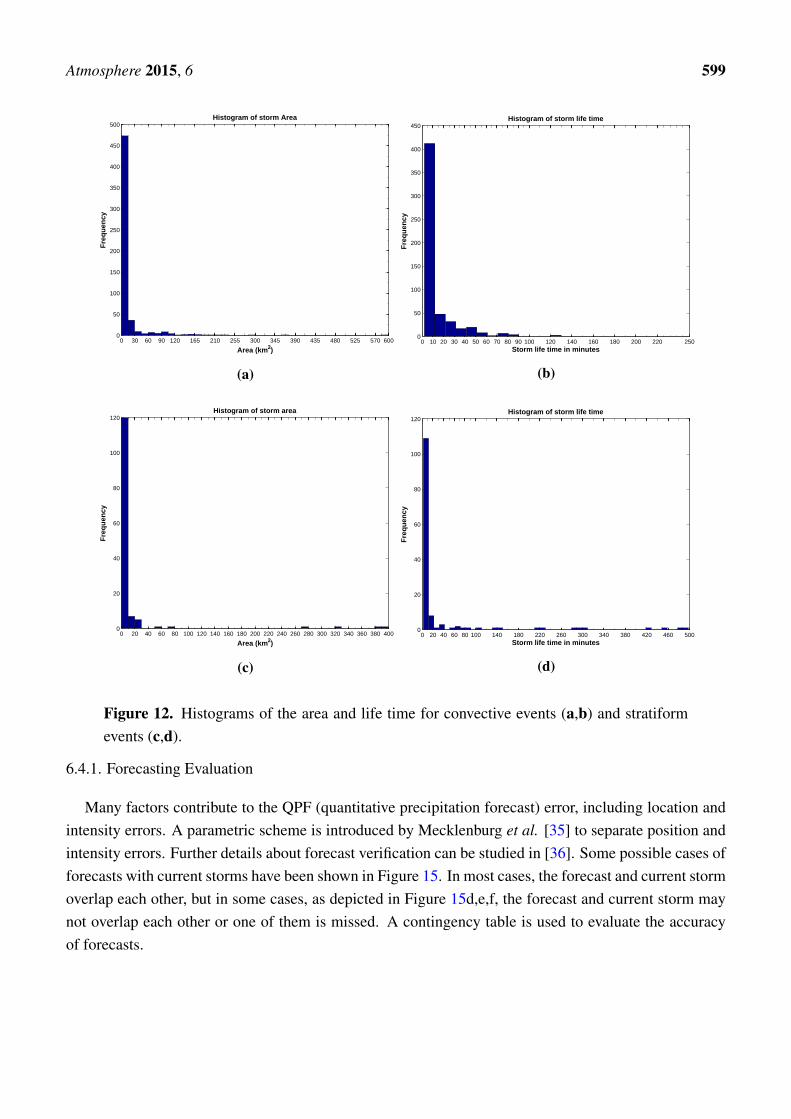
The scatter plot in Figure 11 shows the relationship between the storm’s life time and its area andbetween the velocity and area for both convective and stratiform events. Figure 12b shows that most of


the storms span up to one hour. Figures 11 and 12a reveal that most of the convective storms have lessthan a 30-km2 area with a velocity up to 50 km/h. For the convective storms, the life time may not bethe actual one, because a storm can originate outside the of coverage area of our radar; therefore, thetracking in this case may be partial.

A similar analysis has been performed for stratiform events in Figures 11 and 12c,d. The obtainedresults show that stratiform storms span more than convective storms.

0 50 100 150 200 2500

100

200

300

400

Track life time in minutes

Are

a (k

m2 )

Area vs Life Time for covective events

0 25 50 75 100 125 1500

100

200

300

400

Velocity (km/h)

Are

a (k

m2 )

Area vs Velocity for convective events

0 100 200 300 400 5000

100

200

300

400

Track life time in minutes

Are

a (k

m2 )

Area vs Life Time for stratiform events

0 20 40 60 80 100 1200

100

200

300

400

Velocity (km/h)

Are

a (k

m2 )

Area vs Velocity for stratiform events(a) (b)

(c) (d)

Figure 11. Scatterplots of area vs. life time and area vs. velocity for convective andstratiform events.

6.4. Forecasting

In order to forecast variables of interest, the forecast leading time (FLT) has been set to 5, 10 and15 min. The minimum history required for forecasting is set to 3 min. A five-minute forecast withcorresponding current storms is shown in Figure 13.

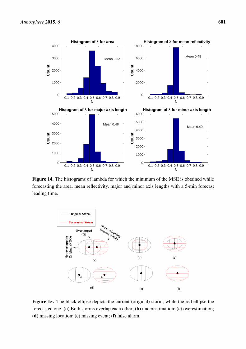
As mentioned in Section 5, all of the variables of interest are forecasted using the second orderexponential smoothing technique. To choose a suitable value for λ in Equations (14) and (15), anautomated criterion is adopted. Higher values of λ provide less smoothing, and the modeled valuesclosely follow the original observation, while lower values for λ provide more smoothing. Figure 14shows that the value of λ is mostly around 0.50 ± 0.02 on average. The results are quite acceptable forbalancing smoothness and following the original observations.


0 30 60 90 120 165 210 255 300 345 390 435 480 525 570 6000

50

100

150

200

250

300

350

400

450

500

Area (km2)

Fre

qu

ency

Histogram of storm Area

(a)

0 10 20 30 40 50 60 70 80 90 100 120 140 160 180 200 220 2500

50

100

150

200

250

300

350

400

450

Storm life time in minutes

Fre

qu

ency

Histogram of storm life time

(b)

0 20 40 60 80 100 120 140 160 180 200 220 240 260 280 300 320 340 360 380 4000

20

40

60

80

100

120

Area (km2)

Fre

qu

ency

Histogram of storm area

(c)

0 20 40 60 80 100 140 180 220 260 300 340 380 420 460 5000

20

40

60

80

100

120

Storm life time in minutes

Fre

qu

ency

Histogram of storm life time

(d)

Figure 12. Histograms of the area and life time for convective events (a,b) and stratiformevents (c,d).

6.4.1. Forecasting Evaluation

Many factors contribute to the QPF (quantitative precipitation forecast) error, including location andintensity errors. A parametric scheme is introduced by Mecklenburg et al. [35] to separate position andintensity errors. Further details about forecast verification can be studied in [36]. Some possible cases offorecasts with current storms have been shown in Figure 15. In most cases, the forecast and current stormoverlap each other, but in some cases, as depicted in Figure 15d,e,f, the forecast and current storm maynot overlap each other or one of them is missed. A contingency table is used to evaluate the accuracyof forecasts.


Figure 13. Forecasted (red) storms with corresponding original storms (black).

A “hit” occurs if the overlapped (O) area is greater than the sum of non-overlapping original (NOO)and non-overlapping forecast (NOF) areas. The rest of the table is filled accordingly if the abovecondition is false. An “underestimate” is recorded if O = 0 and C (current area) is greater than theF (forecasted area). An “overestimate” is counted if F is greater than C and O = 0. A “missed event”describes the case when there is no forecast for the current storm, as depicted in Figure 15e. If both thecurrent storm and forecasted one do not overlap each other, a “missed location” is counted, as shown inFigure 15d. In the case of a “missed location”, the amount of rain forecasted may be underestimated,overestimated or reasonably good. A “false alarm” occurs if the forecasted storm has no matching currentstorm, as shown in Figure 15f.

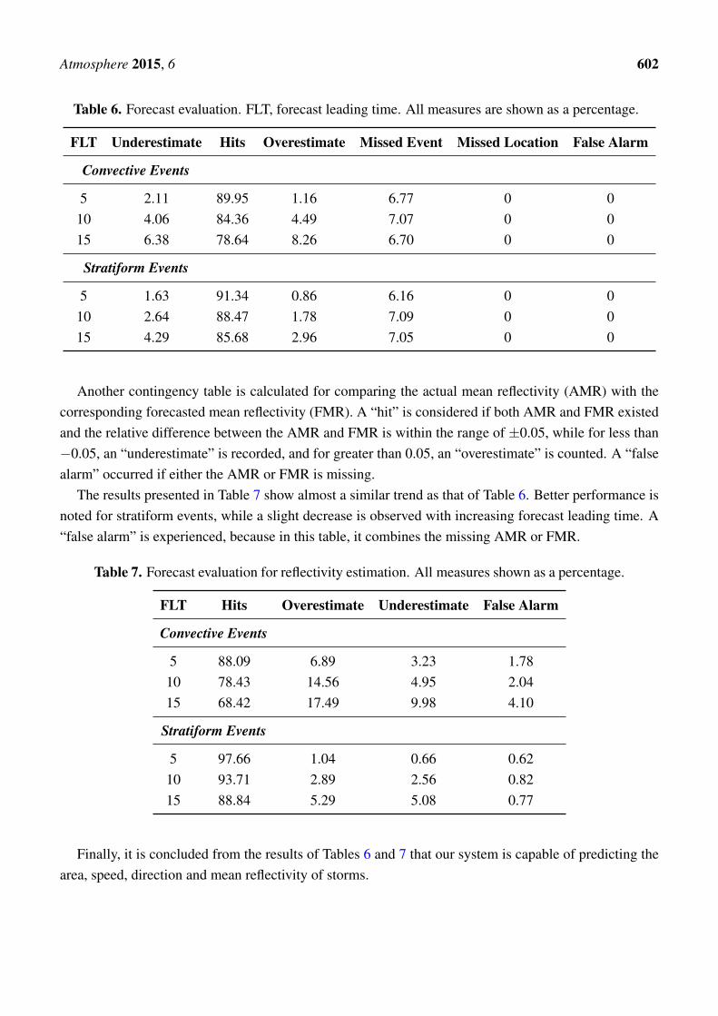
The obtained results are presented in Table 6 showing the positive forecasting capabilities of oursystem. For the stratiform events, a performance increase is noted exactly according to the expectation,because slower and persistent storms can be more easily detected than highly dynamic convective storms.By increasing the forecast leading time (FLT), a slight reduction of the hit rate is experienced, but still,the “hit” rate is good enough for operational needs. The zero “missed location” shows the accuracy ofpredicting the speed and direction of the system. The “missed event” rate is a bit high, but still acceptablefor operational requirements in comparison to the high “hit” rate. Over- and under-estimation of the areahappens rarely. Zero “false alarm” means that the decay of the storms is perfectly predicted, while“missed events” show an early decay in the storm area.


0.1 0.2 0.3 0.4 0.5 0.6 0.7 0.8 0.90

1000

2000

3000

4000

λ

Co

un

t

Histogram of λ for area

0.1 0.2 0.3 0.4 0.5 0.6 0.7 0.8 0.90

2000

4000

6000

8000

λ

Co

un

t

Histogram of λ for mean reflectivity

0.1 0.2 0.3 0.4 0.5 0.6 0.7 0.8 0.90

1000

2000

3000

4000

5000

λ

Co

un

t

Histogram of λ for major axis length

0.1 0.2 0.3 0.4 0.5 0.6 0.7 0.8 0.90

1000

2000

3000

4000

5000

6000

λ

Co

un

t

Histogram of λ for minor axis length

Mean 0.48

Mean 0.48Mean 0.49

Mean 0.52

Figure 14. The histograms of lambda for which the minimum of the MSE is obtained whileforecasting the area, mean reflectivity, major and minor axis lengths with a 5-min forecastleading time.

Figure 15. The black ellipse depicts the current (original) storm, while the red ellipse theforecasted one. (a) Both storms overlap each other; (b) underestimation; (c) overestimation;(d) missing location; (e) missing event; (f) false alarm.


Table 6. Forecast evaluation. FLT, forecast leading time. All measures are shown as a percentage.

FLT Underestimate Hits Overestimate Missed Event Missed Location False Alarm

Convective Events

5 2.11 89.95 1.16 6.77 0 010 4.06 84.36 4.49 7.07 0 015 6.38 78.64 8.26 6.70 0 0

Stratiform Events

5 1.63 91.34 0.86 6.16 0 010 2.64 88.47 1.78 7.09 0 015 4.29 85.68 2.96 7.05 0 0

Another contingency table is calculated for comparing the actual mean reflectivity (AMR) with thecorresponding forecasted mean reflectivity (FMR). A “hit” is considered if both AMR and FMR existedand the relative difference between the AMR and FMR is within the range of ±0.05, while for less than−0.05, an “underestimate” is recorded, and for greater than 0.05, an “overestimate” is counted. A “falsealarm” occurred if either the AMR or FMR is missing.

The results presented in Table 7 show almost a similar trend as that of Table 6. Better performance isnoted for stratiform events, while a slight decrease is observed with increasing forecast leading time. A“false alarm” is experienced, because in this table, it combines the missing AMR or FMR.

Table 7. Forecast evaluation for reflectivity estimation. All measures shown as a percentage.

FLT Hits Overestimate Underestimate False Alarm

Convective Events

5 88.09 6.89 3.23 1.7810 78.43 14.56 4.95 2.0415 68.42 17.49 9.98 4.10

Stratiform Events

5 97.66 1.04 0.66 0.6210 93.71 2.89 2.56 0.8215 88.84 5.29 5.08 0.77

Finally, it is concluded from the results of Tables 6 and 7 that our system is capable of predicting thearea, speed, direction and mean reflectivity of storms.


7. Conclusions

Short-range radars, such as X-band, are quite efficient for monitoring localized rain fall events [37].Rain data collected from MicroRadarNetr presented in [2,3] is used in this investigation. Procedures forall major steps, i.e., storm identification, tracking and nowcasting, of a rain nowcasting system havebeen developed.

Two automatic methods for threshold selection have been tested for storm identification.Each technique is based on the histogram of the image. Inter- and intra-class variances have beencalculated to find the goodness of each automatic threshold technique. The problem of “false merger”has been tackled by using morphological erosion, which shrinks the objects (storms). Sub-storms withinlarge storms have been identified using a multi-threshold technique. Storm identification is evaluated forthe first time.

A novel procedure, called SALdEdA (structure, amplitude, location, eccentricity (circularity)difference and areal difference), has been proposed for storm tracking. Each component of SALdEdAis computed as the normalized difference between volumes, the mean of reflectivity/precipitation,locations, the eccentricities and areas of storms. A global cost function is formulated as the weighted sumof all of these variables. The combinatorial optimization problem is then solved by using the Hungarianalgorithm. The contribution of each component of SALdEdA has been assessed, and recommendationshave been given to assign suitable weights to each component, while computing the cost function. Therange of the possible solution set is constrained further by limiting the distance between the center ofmasses of the two matching storms by introducing a flexible procedure. The “percent correct” techniquesis used for performance evaluation.

A second order exponential smoothing strategy is used. Two contingency tables have been computedto evaluate the accuracy of forecasting. Predicting storm speed, direction and mean reflectivity was akey aspect for the forecasting evaluation.

In the future, the performance of our system will be compared with already developed tools, suchas TITAN [4]. The recently-developed object-based verification method SAL (structure, amplitude andlocation) discussed in [29] will be used to more accurately evaluate the performance of the system.

Author Contributions

The authors contribute equally to this paper.

Conflicts of Interest

The authors declare no conflict of interest.

References

1. Mecklenburg, S.; Jurcxyk, A.; Szturc, J.; Osrodka, K. Quantitative precipitation forecasts(QPF) based on radar data for hydrological models, COST Action 717: Use of radarobservations in hydrological and NWP models. Topic WG1-8, 2002. Available online:http://www.smhi.se/cost717/doc/WDF_01_200203_2.pdf (accessed on 21 April 2015).


2. Gabella, M.; Notarpietro, R.; Bertoldo, S.; Prato, A.; Lucianza, C.; Rorato, O.; Allegretti, M.;Perona, G. A Network of Portable, Low-Cost, X-Band Radars. Available online:http://porto.polito.it/2497341/1/InTech_A_network_of_portable_low_cost_x_band_radars.pdf(accessed on 21 April 2015).

3. Turso, S.; Paolella, S.; Gabella, M.; Perona, G. MicroRadarNet: A network of weather micro radarsfor the identification of local high resolution precipitation patterns. Atmos. Res. 2013, 119, 81–96.

4. Dixon, M.; Wiener, G. TITAN:Thunderstorm Identification, Tracking, Analysis, andNowcasting- A Radar-based Methodology. J. Atmos. and Ocea. Tech. 1993, 6, 785–797.

5. Crane, R. K. Automatic Cell Detection and Tracking. IEEE Trans. Geosci. Electron. 1979,GET-17, 250–262.

6. Lei, H.; Yongguange, W.; Yinjing, L. 3-D Storm Automatic Identification based on MathematicalMorphology. ACTA Meteorol. Sintifica 2009, 23, 156–165.

7. Han, L.; Fu, S.; Zhao, L.; Zheng, Y.; Wang, H.; Lin, Y. 3D Convective Storm Identification,Tracking and Forecasting-An Enhanced TITAN Algorithm. J. Atmos. Oceanic Technol. 2009, 26,719–732.

8. Johnson, J.T.; Mackeen, P.L.; Witt, A.; Mitchell, E.D. Stumpf, G.J.; Eilts, M.D.; Thomas, K.W.The Storm Cell Identification and Tracking Algorithm: An Enhanced WSR-88D Algorithm.Weather Forecast. 1998, 26, 263–276.

9. Gonzalez, R.C.; Woods, R.E. Digital Image Processing, 3rd ed.; Prentice Hall: Upper Saddle River,NJ, USA, 2007.

10. Otsu, N. A Threshold Selection Method from Gray-Level Histograms. IEEE Trans. Syst.Man Cybern. 1979, 9, 62–66.

11. Bjerkaas, C.L.; Forsyth, D.E. Real-time automotive tracking of severe thunderstorms using Dopplerweather radar. In Proceedings of the 11th Conference on Severe Local Storms, Kansas, MO, USA,2–5 October 1979.

12. Handwerker, J. Cell Tracking with TRACE3D-A new algorithm. Atmos. Res. 2002, 61, 15–43.13. Lai, E.S.T. TREC Application in Tropical Cyclone Observation. Available online:

http://www.researchgate.net/publication/228797419_TREC_application_in_tropical_cyclone_observation (accessed on 23 April 2015).

14. Li, L.; Schmid, W. Nowcasting of Motion and Growth of Precipitation with Radar over a ComplexOrography. J. Appl. Meteorol. 1994, 34, 1286–1300.

15. Mathews, J.; Trostel, J. An Improved Storm Cell Identification and Tracking (SCIT) Algorithmbased DBSCAN Cluster and JPDA Tracking Methods. In Proceedings of the InternationalLightning Detection Conference, Orlando, FL, USA, 19–20 April 2010.

16. Rinehart, R.E.; Garvey, E.T. Three-dimensional storm motion detection by conventional weatherradar. Nature 1978, 273, 287–289.

17. Tuttle, J.D.; Foote, G.R. Determination of the boundary layer airflow from a single Doppler radar.J. Atmos. Oceanic Technol. 1998, 7, 2079–2099.

18. Lakshmanan, V.; Hondl, K.; Rabin, R. An Efficient, General-Purpose Technique for IdentifyingStorm Cells in Geospatial Image. J. Atmos. Oceanic Technol. 2009, 26, 523–537.


19. Christos, H.P.; Kenneth,S. Combinatorial Optimization: Algorithms and Complexity, 2nd ed.;Dover Publications, Inc.: Mineola, NY, USA, 1998.

20. Wilson, W.; Crook, N.A.; Mueller, C.K.; Sun, J.; Dixon, M. Nowcasting Thunderstorms: A StatusReport. Bull. Am. Meteo. Soc. 1998, 79, 2079–2099.

21. Keenan, T.; Joe P.; Wilson, J.; Collier, C.; Golding, B.; Burgess, D.; May, P.; Pierce, C.; Bally, J.;Crook, A.; et al. The Sydney 2000 World Weather Research Programme Forecast DemonstrationProject: Overview and Current Status. Bull. Am. Meteor. Soc. 2003, 84, 1041–1054.

22. Lakshmanan, V.; Smith, T. Evaluating a Storm Tracking Algorithm. Available online:https://ams.confex.com/ams/90annual/techprogram/programexpanded_583.htm (accessed on 23April 2015).

23. Bellon, A.; Zawadzki, I.; Kilambi, A.; Lee; H.C.; Lee, Y.H.; Lee, G.McGill Algorithm forPrecipitation Nowcasting by Lagrangian Extrapolation (MAPLE) Applied to the South KoreanRadar Network. Part I: Sensitivity Studies of the Variational Echo Tracking (VET) Technique.Asia-Pacific J. Atmos. Sci. 2010, 46, 369–381.

24. Wilks, D.S. Statistical Methods in the Atmospheric Sciences, 2nd ed.; Elsevier Inc: San Diego, CA,USA, 2006.

25. Lu, J.; Xue, S.; Zhang, X.; Zhang, S.; Lu, W. Neural Fuzzy Inference System-Based WeatherPrediction Model and Its Precipitation Predicting Experiment. Atmosphere 2014, 5, 788–805.

26. Donaldson, J.M.; Dyer, R.M.; Kraus, M.J. An objective evaluation of techniques for predictingsevere weather events. In proceedings of 9th Conference on Severe Local Storm, Norman, OK,USA, 21–23 October 1975.

27. Haralick, R.M.; Shapiro, L.G. Computer and Robot Vision; Addison-Wesley Longman: Boston,MA, USA, 1992.

28. Dixon, M.; Seed, A. Developments in echo tracking-enhancing TITAN. In Proceedings ofthe ERAD2014- The Eighth European Conference on Radar in Meteorology and Hydrology,Garmisch-Partenkirchen, Germany, 1–5 September 2014.

29. Wernli, H.; Paulat, M.; Hagen, M.; Frei, C. SAL- A Novel Quality Measure for the Verification ofQuantitative Precipitation Forecasts. J. AMS 2008, 136, 4470–4487.

30. Shah, S.; Notarpietro, R.; Branca, M. Storm Tracking and Forecasting using High Resolutionechoes of Short Range X-Band Radar. In Proceedings of the ERAD2014- The Eighth EuropeanConference on Radar in Meteorology and Hydrology, Garmisch-Partenkirchen, Germany, 1–5September 2014.

31. Montgomery, D.C.; Jennings, C.L.; Kulahci, M. Introduction to Time Series Analysis andForecasting; Wiley: Hoboken, NJ, USA, 2008.

32. Davini P.; Bechini, R.; Cremonini, R.; Cassardo, C. Radar-Based Analysis of Convective Stormsover Nothwestern Italy. Atmosphere 2012, 3, 33–58.

33. Zhang, H.; Fritts, J.E.; Goldman, S. A. Image segmentation evaluation: A survey of unsupervisedmethods. Comput. Vis. Image Underst. 2008, 110, 260–280.

34. Haralick, R.M.; Shapiro, L.G. Image Segmentation Techniques. Comput. Vis. Gr. Image Proc.1985, 29, 100–132.


35. Mecklenburg, S.; Joss, J.; Schmid, W. Improving the nowcasting of precipitation in an Alpineregion with an enhanced radar echo tracking algorithm. J. Hydrol. 2000, 239, 46–68.

36. Ian, J.; Stephenson, D.B. Forecast Verification, 2nd ed.; Wiley-Blackwell: Chichester, West Sussex,UK, 2012.

37. Allegretti, M.; Bertoldo, S.; Prato, A.; Lucianaz, C.; Rorato, O.; Notarpietro, R.; Gabella, M.X-Band Mini Radar for Observing and Monitoring Rainfall Events. Atmos. Clim. Sci. 2012, 2,290–297.

c⃝ 2015 by the authors; licensee MDPI, Basel, Switzerland. This article is an open access articledistributed under the terms and conditions of the Creative Commons Attribution license(http://creativecommons.org/licenses/by/4.0/).

OPEN ACCESS atmosphere - Semantic Scholar · PDF fileOPEN ACCESS atmosphere ... 22010...

Documents

Transcript of OPEN ACCESS atmosphere - Semantic Scholar · PDF fileOPEN ACCESS atmosphere ... 22010...