arX

iv:1

709.

0471

2v1

[m

ath.

AP]

14

Sep

2017

On the exterior Dirichlet problem for Hessian

quotient equations∗

Dongsheng Li ‡ Zhisu Li (B)†‡

Abstract

In this paper, we establish the existence and uniqueness theorem

for solutions of the exterior Dirichlet problem for Hessian quotient

equations with prescribed asymptotic behavior at infinity. This ex-

tends the previous related results on the Monge-Ampere equations

and on the Hessian equations, and rearranges them in a systematic

way. Based on the Perron’s method, the main ingredient of this paper

is to construct some appropriate subsolutions of the Hessian quotient

equation, which is realized by introducing some new quantities about

the elementary symmetric functions and using them to analyze the

corresponding ordinary differential equation related to the generalized

radially symmetric subsolutions of the original equation.

Keywords: Dirichlet problem, existence and uniqueness, exterior domain,Hessian quotient equation, Perron’s method, prescribed asymptotic behavior,viscosity solution2010 MSC: 35D40, 35J15, 35J25, 35J60, 35J96

1 Introduction

In this paper, we consider the Dirichlet problem for the Hessian quotientequation

σk(λ(D2u))

σl(λ(D2u))= 1 (1.1)

∗This research is supported by NSFC.11671316.†Corresponding author.‡School of Mathematics and Statistics, Xi’an Jiaotong University, Xi’an 710049, China;

Dongsheng Li: lidsh@mail.xjtu.edu.cn; Zhisu Li: lizhisu@stu.xjtu.edu.cn.

1

in the exterior domain Rn \D, where D is a bounded domain in Rn, n ≥ 3,0 ≤ l < k ≤ n, λ(D2u) denotes the eigenvalue vector λ := (λ1, λ2, ..., λn) ofthe Hessian matrix D2u of the function u, and

σ0(λ) ≡ 1 and σj(λ) :=∑

1≤s1<s2<...<sj≤n

λs1λs2...λsj (∀1 ≤ j ≤ n)

are the elementary symmetric functions of the n-vector λ. Note that whenl = 0, (1.1) is the Hessian equation σk(λ(D

2u)) = 1; when l = 0, k = 1, it isthe Poisson equation ∆u = 1, a linear elliptic equation; when l = 0, k = n, itis the famous Monge-Ampere equation det(D2u) = 1; and when l = 1, k = 3,n = 3 or 4, it is the special Lagrangian equation σ1(λ(D

2u)) = σ3(λ(D2u)) in

three or four dimension (in three dimension, this is det(D2u) = ∆u indeed)which arises from the special Lagrangian geometry [HL82].

For linear elliptic equations of second order, there have been much exten-sive studies on the exterior Dirichlet problem, see [MS60] and the referencestherein. For the Monge-Ampere equation, a classical theorem of Jorgens[Jor54], Calabi [Cal58] and Pogorelov [Pog72] states that any convex classi-cal solution of det(D2u) = 1 in Rn must be a quadratic polynomial. Relatedresults was also given by [CY86], [Caf95], [TW00] and [JX01]. Caffarelli andLi [CL03] extended the Jorgens-Calabi-Pogorelov theorem to exterior do-mains. They proved that if u is a convex viscosity solution of det(D2u) = 1in the exterior domain Rn \D, where D is a bounded domain in Rn, n ≥ 3,then there exist A ∈ Rn×n, b ∈ Rn and c ∈ R such that

lim sup|x|→+∞

|x|n−2

∣∣∣∣u(x)−(1

2xTAx+ bTx+ c

)∣∣∣∣ <∞. (1.2)

With such prescribed asymptotic behavior at infinity, they also established anexistence and uniqueness theorem for solutions of the Dirichlet problem of theMonge-Ampere equation in the exterior domain of Rn, n ≥ 3. See [FMM99],[FMM00] or [Del92] for similar problems in two dimension. Recently, J.-G. Bao, H.-G. Li and Y.-Y. Li [BLL14] extended the above existence anduniqueness theorem of the exterior Dirichlet problem in [CL03] for the Monge-Ampere equation to the Hessian equation σk(λ(D

2u)) = 1 with 2 ≤ k ≤ nand with some appropriate prescribed asymptotic behavior at infinity whichis modified from (1.2). Before them, for the special case that A = c0I withc0 := (Ck

n)−1/k and Ck

n := n!/(k!(n− k)!), the exterior Dirichlet problem forthe Hessian equation has been investigated by Dai and Bao in [DB11]. At the

2

same time, Dai [Dai11] proved the existence theorem of the exterior Dirichletproblem for the Hessian quotient equation (1.1) with k− l ≥ 3, and with theprescribed asymptotic behavior at infinity of the special case that A = c∗I,that is,

lim sup|x|→+∞

|x|k−l−2∣∣∣u(x)−

(c∗2|x|2 + c

)∣∣∣ <∞, (1.3)

where

c∗ :=

(C l

n

Ckn

) 1

k−l

with C in :=

n!

i!(n− i)!for i = k, l. (1.4)

As they pointed out in [LB14] that the restriction k− l ≥ 3 rules out an im-portant example, the special Lagrangian equation det(D2u) = ∆u in threedimension. Later, [LD12] improve the result in [Dai11] for (1.1) with k−l ≥ 3to that for (1.1) with 0 ≤ l < k ≤ (n + 1)/2. More recently, Li and Bao[LB14] established the existence theorem of the exterior Dirichlet problemfor a class of fully nonlinear elliptic equations related to the eigenvalues ofthe Hessian which include the Monge-Ampere equations, Hessian equations,Hessian quotient equations and the special Lagrangian equations in dimen-sion equal and lager than three, but with the prescribed asymptotic behaviorat infinity only in the special case of (1.2) that A = c∗I with c∗ some ap-propriate constant, like (1.3) and (1.4).

In this paper, we focus our attention on the Hessian quotient equation(1.1) and establish the existence and uniqueness theorem for the exteriorDirichlet problem of it with prescribed asymptotic behavior at infinity of thetype similar to (1.2). This extends the previous corresponding results onthe Monge-Ampere equations [CL03] and on the Hessian equations [BLL14]to Hessian quotient equations, and also extends those results on the Hessianquotient equations in [Dai11], [LD12] and [LB14] to be valid for generalprescribed asymptotic behavior condition at infinity. Since we do not restrictourselves to the case k−l ≥ 3 or 0 ≤ l < k ≤ (n+1)/2 only, our theorems alsoapply to the special Lagrangian equations det(D2u) = ∆u in three dimensionand σ1(λ(D

2u)) = σ3(λ(D2u)) in four dimension. Indeed, we will show in

our forthcoming paper [LL16] that our method still works very well for thespecial Lagrangian equations with higher dimension and with general phase.

We would like to remark that, for the interior Dirichlet problems therehave been much extensive studies, see for example [CIL92], [CNS85], [Ivo85],[Kry83], [Urb90], [Tru90] and [Tru95]; see [BCGJ03] and the references given

3

there for more on the Hessian quotient equations; and for more on the spe-cial Lagrangian equations, we refer the reader to [HL82], [Fu98], [Yuan02],[CWY09] and the references therein.

For the reader’s convenience, we give the following definitions relatedto Hessian quotient equation (see also [CIL92], [CC95], [CNS85], [Tru90],[Tru95] and the references therein).

We say that a function u ∈ C2(R

n \D)is k-convex, if λ(D2u) ∈ Γk

in Rn \ D, where Γk is the connected component of λ ∈ Rn|σk(λ) > 0containing the positive cone

Γ+ := λ ∈ Rn|λi > 0, ∀i = 1, 2, ..., n .

It is well known that Γk is an open convex symmetric cone with its vertex atthe origin and that

Γk = λ ∈ Rn|σj(λ) > 0, ∀j = 1, 2, ..., k ,

which implies

λ ∈ Rn|λ1 + λ2 + ... + λn > 0 = Γ1 ⊃ ... ⊃ Γk ⊃ Γk+1 ⊃ ... ⊃ Γn = Γ+

with the first term Γ1 the half space and with the last term Γn the positivecone Γ+. Furthermore, we also know that

∂λiσj(λ) > 0, ∀1 ≤ i ≤ n, ∀1 ≤ j ≤ k, ∀λ ∈ Γk, ∀1 ≤ k ≤ n (1.5)

(see [CNS85] or [Urb90] for more details).Let Ω be an open domain in Rn and let f ∈ C0(Ω) be nonnegative.

Suppose 0 ≤ l < k ≤ n. A function u ∈ C0(Ω) is said to be a viscositysubsolution of

σk(λ(D2u))

σl(λ(D2u))= f in Ω (1.6)

(or say that u satisfies

σk(λ(D2u))

σl(λ(D2u))≥ f in Ω

in the viscosity sense, similarly hereinafter), if for any function v ∈ C2(Ω)

and any point x∗ ∈ Ω satisfying

v(x) ≥ u(x), ∀x ∈ Ω and v(x∗) = u(x∗),

4

we haveσk(λ(D

2v))

σl(λ(D2v))≥ f in Ω.

A function u ∈ C0(Ω) is said to be a viscosity supersolution of (1.6) if forany k-convex function v ∈ C2(Ω) and any point x∗ ∈ Ω satisfying

v(x) ≤ u(x), ∀x ∈ Ω and v(x∗) = u(x∗),

we haveσk(λ(D

2v))

σl(λ(D2v))≤ f in Ω.

A function u ∈ C0(Ω) is said to be a viscosity solution of (1.6), if it isboth a viscosity subsolution and a viscosity supersolution of (1.6). A func-tion u ∈ C0(Ω) is said to be a viscosity subsolution (respectively, superso-lution, solution) of (1.6) and u = ϕ on ∂Ω with some ϕ ∈ C0(∂Ω), if uis a viscosity subsolution (respectively, supersolution, solution) of (1.6) andu ≤(respectively, ≥,=)ϕ on ∂Ω.

Note that in the definitions of viscosity solution above, we have used theellipticity of the Hessian quotient equations indeed. For completeness andconvenience, this will be proved in the end of Subsection 2.3. See also [CC95],[CIL92], [CNS85], [Urb90] and the references therein.

Define

Ak,l :=A ∈ S(n)

∣∣λ(A) ∈ Γ+, σk(λ(A)) = σl(λ(A)).

Note that there are plenty of elements in Ak,l. In fact, for any A ∈ S(n) withλ(A) ∈ Γ+, if we set

:=

(σk(λ(A))

σl(λ(A))

)− 1

k−l

,

we then have A ∈ Ak,l. Let

Ak,l :=A ∈ Ak,l

∣∣mk,l(λ(A)) > 2,

where mk,l(λ) is a quantity which plays an important role in this paper. Wewill give the specific definition of mk,l(λ) in (2.1) in Subsection 2.2, and

verify there that Ak,l possesses the following fine properties.

Proposition 1.1. Suppose 0 ≤ l < k ≤ n and n ≥ 3.

5

(1) If k − l ≥ 2, then Ak,l = Ak,l.

(2) An,0 = An,0 and mn,0 ≡ n.

(3) c∗I ∈ Ak,l and mk,l(c∗(1, 1, ..., 1)) = n, where c∗ is the one defined in(1.4).

The main result of this paper now can be stated as below.

Theorem 1.1. Let D be a bounded strictly convex domain in Rn, n ≥ 3,

∂D ∈ C2 and let ϕ ∈ C2(∂D). Then for any given A ∈ Ak,l with 0 ≤ l <k ≤ n, and any given b ∈ Rn, there exists a constant c depending only onn,D, k, l, A, b and ‖ϕ‖C2(∂D), such that for every c ≥ c, there exists a unique

viscosity solution u ∈ C0(Rn \D) of

σk(λ(D2u))

σl(λ(D2u))= 1 in Rn \D,

u = ϕ on ∂D,

lim sup|x|→+∞

|x|m−2

∣∣∣∣u(x)−(1

2xTAx+ bTx+ c

)∣∣∣∣ <∞,

(1.7)

where m ∈ (2, n] is a constant depending only on n, k, l and λ(A), whichactually can be taken as mk,l(λ(A)).

Remark 1.1. (1) One can easily see that Theorem 1.1 still holds with A ∈Ak,l replaced by A ∈ A

∗k,l and λ(A) replaced by λ(A∗), where

A∗k,l :=

A ∈ Rn×n

∣∣λ(A∗) ∈ Γ+, σk(λ(A∗)) = σl(λ(A

∗)), mk,l(λ(A∗)) > 2

and A∗ := (A + AT )/2. This is to say that the above theorem can beadapted to a slightly more general form by modifying the meaning of

Ak,l.

(2) For the special cases that l = 0 (i.e., the Hessian equation σk(λ(D2u)) =

1) and that l = 0 and k = n (i.e., the Monge-Ampere equation det(D2u) =1), in view of Proposition 1.1-(2), our Theorem 1.1 recovers the corre-sponding results [BLL14, Theorem 1.1] and [CL03, Theorem 1.5], respec-tively.

6

(3) For A = c∗I with c∗ defined in (1.4), by Proposition 1.1-(1),(3), ourresults improve those in [Dai11] and [LD12]. Indeed, by Proposition 1.1-(3), the main results in [Dai11], [LD12] and those parts concerningthe Hessian quotient equations in [LB14] can all be recovered by Theo-rem 1.1 as special cases. Furthermore, our results also apply to the specialLagrangian equation det(D2u) = ∆u in three dimension (respectively,σ1(λ(D

2u)) = σ3(λ(D2u)) in four dimension), not only for A =

√3I

(respectively, A = I), but also for any A ∈ A3,1.

The paper is organized as follows. In Section 2, after giving some basicnotations in Subsection 2.1, we introduce the definitions of Ξk, ξk, ξk andmk,l, and investigate their properties in Subsection 2.2. Then we collect inSubsection 2.3 some preliminary lemmas which will be used in this paper.Section 3 is devoted to the proof of the main theorem (Theorem 1.1). To dothis, we start in Subsection 3.1 to construct some appropriate subsolutions ofthe Hessian quotient equation (1.1), by taking advantages of the propertiesof Ξk, ξk, ξk andmk,l explored in Subsection 2.2. Then in Subsection 3.2, afterreducing Theorem 1.1 to Lemma 3.3 by simplification and normalization, weprove Lemma 3.3 by applying the Perron’s method to the subsolutions weconstructed in Subsection 3.1.

2 Preliminary

2.1 Notation

In this paper, S(n) denotes the linear space of symmetric n × n realmatrices, and I denotes the identity matrix.

For anyM ∈ S(n), ifm1, m2, ..., mn are the eigenvalues ofM (usually, theassumption m1 ≤ m2 ≤ ... ≤ mn is added for convenience), we will denotethis fact briefly by λ(M) = (m1, m2, ..., mn) and call λ(M) the eigenvaluevector of M .

For A ∈ S(n) and ρ > 0, we denote by

Eρ :=x ∈ Rn

∣∣xTAx < ρ2=x ∈ Rn

∣∣rA(x) < ρ

the ellipsoid of size ρ with respect to A, where we set rA(x) :=√xTAx.

7

For any p ∈ Rn, we write

σk(p) :=∑

1≤s1<s2<...<sk≤n

ps1ps2...psk (∀1 ≤ k ≤ n)

as the k-th elementary symmetric function of p. Meanwhile, we will adoptthe conventions that σ−1(p) ≡ 0, σ0(p) ≡ 1 and σk(p) ≡ 0, ∀k ≥ n + 1; andwe will also define

σk;i(p) :=(σk(λ)

∣∣λi=0

) ∣∣∣λ=p

= σk (p1, p2, ..., pi, ..., pn)

for any −1 ≤ k ≤ n and any 1 ≤ i ≤ n, and similarly

σk;i,j(p) :=(σk(λ)

∣∣λi=λj=0

) ∣∣∣λ=p

= σk (p1, p2, ..., pi, ..., pj , ..., pn)

for any −1 ≤ k ≤ n and any 1 ≤ i, j ≤ n, i 6= j, for convenience.

2.2 Definitions and properties of Ξk, ξk, ξk and mk,l

To establish the existence of the solution of (1.1), by the Perron’s method,the key point is to find some appropriate subsolutions of the equation. Sincethe Hessian quotient equation (1.1) is a highly fully nonlinear equation whichincluding polynomials of the eigenvalues of the the Hessian matrixD2u, σk(λ)and σl(λ), of different order of homogeneities, to solve it we need to strikea balance between them. It will turn out to be clear that the quantitiesΞk, ξk, ξk and mk,l, which we shall introduce below, are very natural andperfectly fit for this purpose.

Definition 2.1. For any 0 ≤ k ≤ n and any a ∈ Rn \ 0, let

Ξk := Ξk(a, x) :=

∑ni=1 σk−1;i(a)a

2ix

2i

σk(a)∑n

i=1 aix2i

, ∀x ∈ Rn \ 0,

and defineξk := ξk(a) := sup

x∈Rn\0

Ξk(a, x)

andξk:= ξ

k(a) := inf

x∈Rn\0Ξk(a, x).

8

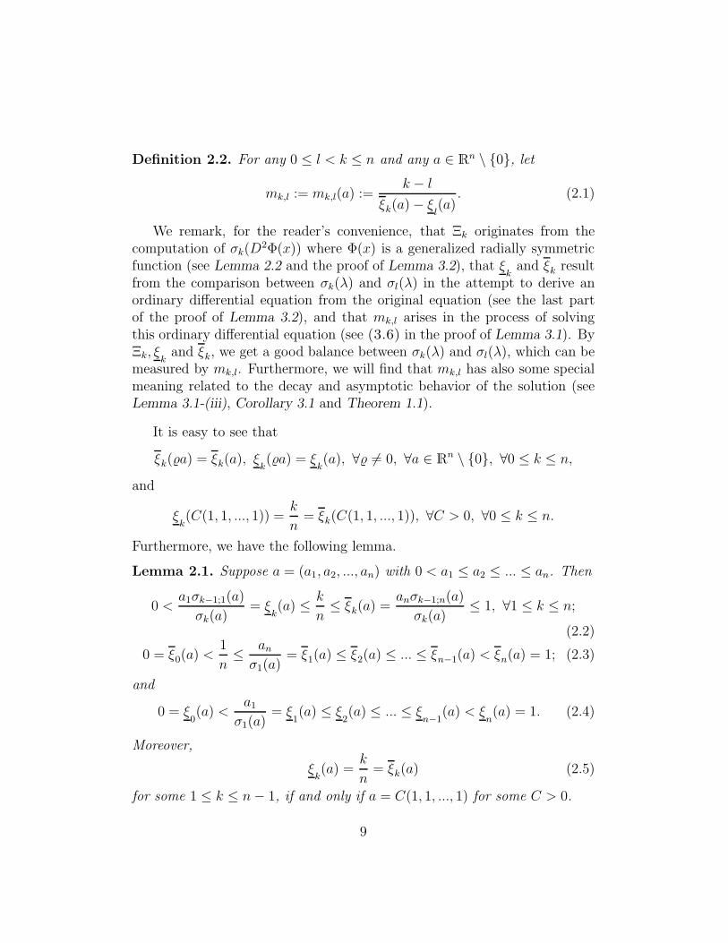
Definition 2.2. For any 0 ≤ l < k ≤ n and any a ∈ Rn \ 0, let

mk,l := mk,l(a) :=k − l

ξk(a)− ξl(a)

. (2.1)

We remark, for the reader’s convenience, that Ξk originates from thecomputation of σk(D

2Φ(x)) where Φ(x) is a generalized radially symmetricfunction (see Lemma 2.2 and the proof of Lemma 3.2), that ξ

kand ξk result

from the comparison between σk(λ) and σl(λ) in the attempt to derive anordinary differential equation from the original equation (see the last partof the proof of Lemma 3.2), and that mk,l arises in the process of solvingthis ordinary differential equation (see (3.6) in the proof of Lemma 3.1). ByΞk, ξk and ξk, we get a good balance between σk(λ) and σl(λ), which can bemeasured by mk,l. Furthermore, we will find that mk,l has also some specialmeaning related to the decay and asymptotic behavior of the solution (seeLemma 3.1-(iii), Corollary 3.1 and Theorem 1.1).

It is easy to see that

ξk(a) = ξk(a), ξk(a) = ξk(a), ∀ 6= 0, ∀a ∈ Rn \ 0, ∀0 ≤ k ≤ n,

and

ξk(C(1, 1, ..., 1)) =

k

n= ξk(C(1, 1, ..., 1)), ∀C > 0, ∀0 ≤ k ≤ n.

Furthermore, we have the following lemma.

Lemma 2.1. Suppose a = (a1, a2, ..., an) with 0 < a1 ≤ a2 ≤ ... ≤ an. Then

0 <a1σk−1;1(a)

σk(a)= ξ

k(a) ≤ k

n≤ ξk(a) =

anσk−1;n(a)

σk(a)≤ 1, ∀1 ≤ k ≤ n;

(2.2)

0 = ξ0(a) <1

n≤ anσ1(a)

= ξ1(a) ≤ ξ2(a) ≤ ... ≤ ξn−1(a) < ξn(a) = 1; (2.3)

and

0 = ξ0(a) <

a1σ1(a)

= ξ1(a) ≤ ξ

2(a) ≤ ... ≤ ξ

n−1(a) < ξ

n(a) = 1. (2.4)

Moreover,

ξk(a) =

k

n= ξk(a) (2.5)

for some 1 ≤ k ≤ n− 1, if and only if a = C(1, 1, ..., 1) for some C > 0.

9

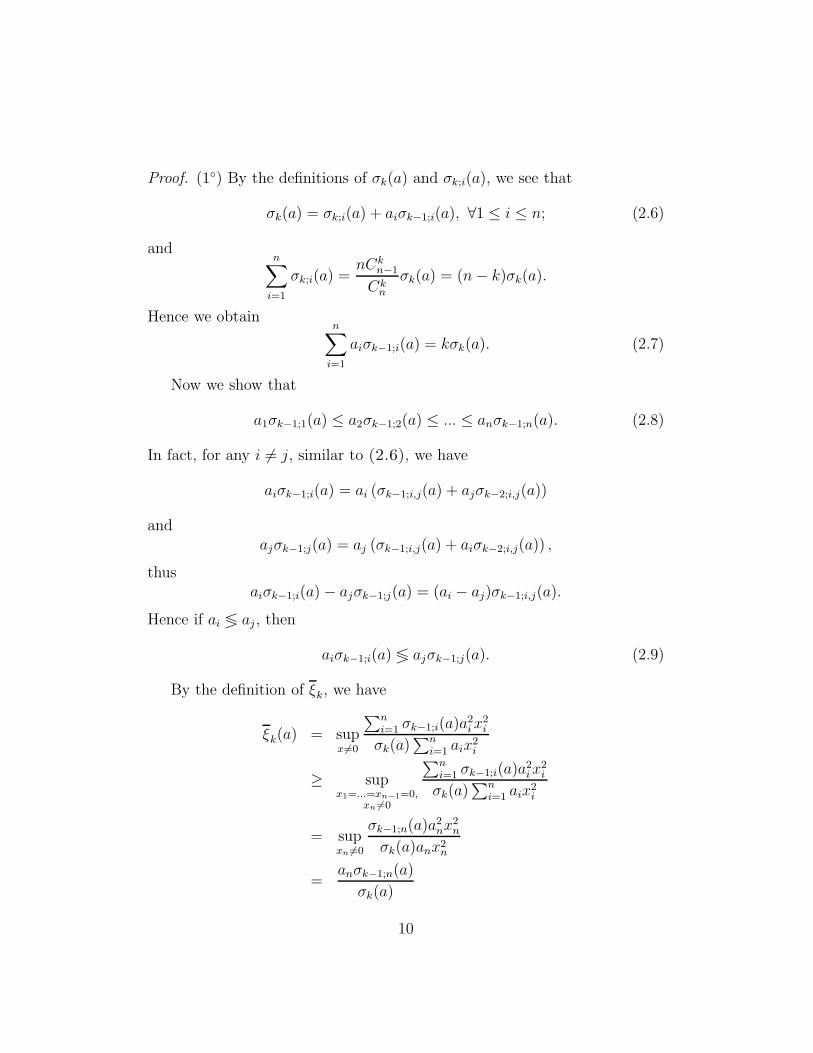
Proof. (1) By the definitions of σk(a) and σk;i(a), we see that

σk(a) = σk;i(a) + aiσk−1;i(a), ∀1 ≤ i ≤ n; (2.6)

andn∑

i=1

σk;i(a) =nCk

n−1

Ckn

σk(a) = (n− k)σk(a).

Hence we obtainn∑

i=1

aiσk−1;i(a) = kσk(a). (2.7)

Now we show that

a1σk−1;1(a) ≤ a2σk−1;2(a) ≤ ... ≤ anσk−1;n(a). (2.8)

In fact, for any i 6= j, similar to (2.6), we have

aiσk−1;i(a) = ai (σk−1;i,j(a) + ajσk−2;i,j(a))

andajσk−1;j(a) = aj (σk−1;i,j(a) + aiσk−2;i,j(a)) ,

thusaiσk−1;i(a)− ajσk−1;j(a) = (ai − aj)σk−1;i,j(a).

Hence if ai ≶ aj , then

aiσk−1;i(a) ≶ ajσk−1;j(a). (2.9)

By the definition of ξk, we have

ξk(a) = supx 6=0

∑ni=1 σk−1;i(a)a

2ix

2i

σk(a)∑n

i=1 aix2i

≥ supx1=...=xn−1=0,

xn 6=0

∑ni=1 σk−1;i(a)a

2ix

2i

σk(a)∑n

i=1 aix2i

= supxn 6=0

σk−1;n(a)a2nx

2n

σk(a)anx2n

=anσk−1;n(a)

σk(a)

10

and

ξk(a) = supx 6=0

∑ni=1 σk−1;i(a)a

2ix

2i

σk(a)∑n

i=1 aix2i

≤ supx 6=0

anσk−1;n(a)∑n

i=1 aix2i

σk(a)∑n

i=1 aix2i

by (2.8)

=anσk−1;n(a)

σk(a).

Hence we obtain

ξk(a) =anσk−1;n(a)

σk(a). (2.10)

Similarly

ξk(a) =

a1σk−1;1(a)

σk(a). (2.11)

From (2.7), we have

n∑

i=1

aiσk−1;i(a)

σk(a)= k.

Combining this with (2.8), (2.10) and (2.11), we deduce that

ξk(a) ≤ k

n≤ ξk(a).

Thus the proof of (2.2) is complete, and (2.5) is also clear in view of (2.9).

(2) Since it follows from (2.6) that

aiσk−1;i(a) < σk(a), ∀1 ≤ i ≤ n, ∀1 ≤ k ≤ n− 1,

we obtainξk(a) ≤ ξk(a) < 1, ∀0 ≤ k ≤ n− 1.

On the other hand, we have ξn(a) = ξn(a) = 1 which follows from

aiσn−1;i(a) = σn(a), ∀1 ≤ i ≤ n.

Combining (2.10) and (2.6), we discover that

ξk(a) =anσk−1;n(a)

σk(a)=

anσk−1;n(a)

σk;n(a) + anσk−1;n(a)

11

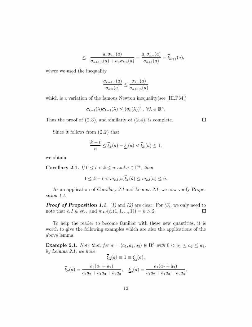
≤ anσk;n(a)

σk+1;n(a) + anσk;n(a)=anσk;n(a)

σk+1(a)= ξk+1(a),

where we used the inequality

σk−1;n(a)

σk;n(a)≤ σk;n(a)

σk+1;n(a)

which is a variation of the famous Newton inequality(see [HLP34])

σk−1(λ)σk+1(λ) ≤ (σk(λ))2 , ∀λ ∈ Rn.

Thus the proof of (2.3), and similarly of (2.4), is complete.

Since it follows from (2.2) that

k − l

n≤ ξk(a)− ξ

l(a) < ξk(a) ≤ 1,

we obtain

Corollary 2.1. If 0 ≤ l < k ≤ n and a ∈ Γ+, then

1 ≤ k − l < mk,l(a)ξk(a) ≤ mk,l(a) ≤ n.

As an application of Corollary 2.1 and Lemma 2.1, we now verify Propo-sition 1.1.

Proof of Proposition 1.1. (1) and (2) are clear. For (3), we only need tonote that c∗I ∈ Ak,l and mk,l(c∗(1, 1, ..., 1)) = n > 2.

To help the reader to become familiar with these new quantities, it isworth to give the following examples which are also the applications of theabove lemma.

Example 2.1. Note that, for a = (a1, a2, a3) ∈ R3 with 0 < a1 ≤ a2 ≤ a3,by Lemma 2.1, we have

ξ3(a) ≡ 1 ≡ ξ3(a),

ξ2(a) =a3(a1 + a2)

a1a2 + a1a3 + a2a3, ξ

2(a) =

a1(a2 + a3)

a1a2 + a1a3 + a2a3,

12

ξ1(a) =a3

a1 + a2 + a3, ξ

1(a) =

a1a1 + a2 + a3

,

andξ0(a) ≡ 0 ≡ ξ

0(a).

Thus we can compute, for a = (1, 2, 3), that

ξ2 =9

11, ξ

2=

5

11, ξ1 =

1

2, ξ

1=

1

6,

m3,2 =11

6< 2, m3,1 =

12

5> 2, m3,0 ≡ 3 > 2,

m2,1 =66

43< 2, m2,0 =

22

9> 2 and m1,0 = 2,

and, for a = (11, 12, 13), that

ξ2 =299

431, ξ

2=

275

431, ξ1 =

13

36, ξ

1=

11

36,

m3,2 =431

156> 2, m3,1 =

72

25> 2, m3,0 ≡ 3 > 2,

m2,1 =15516

6023> 2, m2,0 =

862

299> 2 and m1,0 =

36

13> 2.

Remark 2.1. (1) By definition of mk,l, we can easily check that for any1 < k ≤ n, mk,k−1(a) > 2 if and only if ξ

k−1(a) ≤ ξk(a) ≤ ξ

k−1(a)+1/2.

This will show us how mk,l plays a role in the making of a balance betweendifferent order of homogeneities as we stated in the beginning of thissubsection.

(2) Proposition 1.1-(1) states that Ak,l = Ak,l provided k − l ≥ 2. Note that

this is the best case we can expect, since in general Ak,k−1 $ Ak,k−1,which is evident by the fact stated in the first item of this remark (andalso by the above examples). For example, in R3 we have

m3,2(a) > 2 ⇔ ξ3(a) ≤ ξ2(a) + 1/2 ⇔ a1 >

a2a3a2 + a3

,

where the last inequality is not always true.

13

2.3 Some preliminary lemmas

In this subsection, we collect some preliminary lemmas which will bemainly used in Section 3.

We first give a lemma to compute σk(λ(M)) with M of certain type. IfΦ(x) := φ(r) with φ ∈ C2, r =

√xTAx, A ∈ S(n) ∩ Γ+ and a = λ(A)

(we may call Φ a generalized radially symmetric function with respect to A,according to [BLL14]), one can conclude that

∂ijΦ(x) =φ′(r)

raiδij +

φ′′(r)− φ′(r)r

r2(aixi)(ajxj), ∀1 ≤ i, j ≤ n,

provided A is normalized to a diagonal matrix (see the first part of Subsec-tion 3.2 and the proof of Lemma 3.2 for details). As far as we know, generallythere is no explicit formula for λ(D2Φ(x)) of this type, but luckily we havea method to calculate σk (λ(D

2Φ(x))) for each 1 ≤ k ≤ n, which can bepresented as follows.

Lemma 2.2. If M = (piδij + sqiqj)n×n with p, q ∈ Rn and s ∈ R, then

σk (λ(M)) = σk(p) + sn∑

i=1

σk−1;i(p)q2i , ∀1 ≤ k ≤ n.

Proof. See [BLL14].

To process information on the boundary we need the following lemma.

Lemma 2.3. Let D be a bounded strictly convex domain of Rn, n ≥ 2,∂D ∈ C2, ϕ ∈ C0(D) ∩ C2(∂D) and let A ∈ S(n), detA 6= 0. Then thereexists a constant K > 0 depending only on n, diamD, the convexity of D,‖ϕ‖C2(D), the C

2 norm of ∂D and the upper bound of A, such that for anyξ ∈ ∂D, there exists x(ξ) ∈ Rn satisfying

|x(ξ)| ≤ K and Qξ(x) < ϕ(x), ∀x ∈ D \ ξ,

where

Qξ(x) :=1

2(x− x(ξ))T A (x− x(ξ))−1

2(ξ − x(ξ))T A (ξ − x(ξ))+ϕ(ξ), ∀x ∈ Rn.

14

Proof. See [CL03] or [BLL14].

Remark 2.2. It is easy to check that Qξ satisfy the following properties.

(1) Qξ ≤ ϕ on D and Qξ(ξ) = ϕ(ξ).

(2) If A ∈ Ak,l, thenσk(λ(D

2Qξ))

σl(λ(D2Qξ))= 1 in Rn.

(3) There exists c = c(D,A,K) > 0 such that

Qξ(x) ≤1

2xTAx+ c, ∀x ∈ ∂D, ∀ξ ∈ ∂D.

Now we introduce the following well known lemmas about the comparisonprinciple and Perron’s method which will be applied to the Hessian quotientequations but stated in a slightly more general setting. These lemmas areadaptions of those appeared in [CNS85] [Jen88] [Ish89] [Urb90] and [CIL92].For specific proof of them one may also consult [BLL14] and [LB14].

Lemma 2.4 (Comparison principle). Assume Γ+ ⊂ Γ ⊂ Rn is an open

convex symmetric cone with its vertex at the origin, and suppose f ∈ C1(Γ)and fλi

(λ) > 0, ∀λ ∈ Γ, ∀i = 1, 2, ..., n. Let Ω ⊂ Rn be a domain and let

u, u ∈ C0(Ω) satisfying

f(λ(D2u

))≥ 1 ≥ f

(λ(D2u

))

in Ω in the viscosity sense. Suppose u ≤ u on ∂Ω (and additionally

lim|x|→+∞

(u− u) (x) = 0

provided Ω is unbounded). Then u ≤ u in Ω.

Lemma 2.5 (Perron’s method). Assume that Γ+ ⊂ Γ ⊂ Rn is an open

convex symmetric cone with its vertex at the origin, and suppose f ∈ C1(Γ)and fλi

(λ) > 0, ∀λ ∈ Γ, ∀i = 1, 2, ..., n. Let Ω ⊂ Rn be a domain, ϕ ∈

C0(∂Ω) and let u, u ∈ C0(Ω) satisfying

f(λ(D2u

))≥ 1 ≥ f

(λ(D2u

))

15

in Ω in the viscosity sense. Suppose u ≤ u in Ω, u = ϕ on ∂Ω (and addi-tionally

lim|x|→+∞

(u− u) (x) = 0

provided Ω is unbounded). Then

u(x) := supv(x)

∣∣v ∈ C0(Ω), u ≤ v ≤ u in Ω, f(λ(D2v

))≥ 1 in Ω

in the viscosity sense, v = ϕ on ∂Ω

is the unique viscosity solution of the Dirichlet problem

f(λ(D2u

))= 1 in Ω,

u = ϕ on ∂Ω.

Remark 2.3. In order to apply the above lemmas to the Hessian quotientoperator

f(λ) :=σk(λ)

σl(λ)

in the cone Γ := Γk, we need to show that

∂λi

(σk(λ)

σl(λ)

)> 0, ∀1 ≤ i ≤ n, ∀0 ≤ l < k ≤ n, ∀λ ∈ Γk, (2.12)

which indeed indicates that the Hessian quotient equations (1.1) are ellipticequations with respect to its k-convex solution u.

Indeed, for l = 0, (2.12) is clear in light of (1.5). For 1 ≤ l < k ≤ n,since

∂λiσk(λ) =

σk(λ)− σk;i(λ)

λi= σk−1;i(λ)

according to (2.6), we have

∂λi

(σk(λ)

σl(λ)

)=σk−1;i(λ)σl(λ)− σk(λ)σl−1;i(λ)

(σl(λ))2.

Thus to prove (2.12), it remains to verify

σk−1;i(λ)σl(λ) ≥ σk(λ)σl−1;i(λ).

16

In view of (2.6), this is equivalent to

σk−1;i(λ)σl;i(λ) ≥ σk;i(λ)σl−1;i(λ),

which in turn is equivalent to

σl;i(λ)

σl−1;i(λ)≥ σk;i(λ)

σk−1;i(λ),

since σj;i(λ) = ∂λiσj+1(λ) > 0, ∀1 ≤ i ≤ n, ∀0 ≤ j ≤ k − 1, ∀λ ∈ Γk,

according to (1.5). For the proof of the latter, we only need to note that

σj;i(λ)

σj−1;i(λ)≥ σj+1;i(λ)

σj;i(λ),

which is the variation of the Newton inequality(see [HLP34])

σj−1(λ)σj+1(λ) ≤ (σj(λ))2 , ∀λ ∈ Rn,

as we met in the proof of Lemma 2.1.

3 Proof of the main theorem

3.1 Construction of the subsolutions

The purpose of this subsection is to prove the following key lemma andthen use it to construct subsolutions of (1.1). We remark that for the gen-eralized radially symmetric subsolution Φ(x) = φ(r) that we intend to con-struct, the solution ψ(r) discussed in the the following lemma actually isequivalent to φ′(r)/r (see the proof of the Lemma 3.2).

Lemma 3.1. Let 0 ≤ l < k ≤ n, n ≥ 3, A ∈ Ak,l, a := (a1, a2, ..., an) :=λ(A), 0 < a1 ≤ a2 ≤ ... ≤ an and β ≥ 1. Then the problem

ψ(r)k + ξk(a)rψ(r)k−1ψ′(r)

−ψ(r)l − ξl(a)rψ(r)l−1ψ′(r) = 0, r > 1,

ψ(1) = β,

(3.1)

has a unique smooth solution ψ(r) = ψ(r, β) on [1,+∞), which satisfies

17

(i) 1 ≤ ψ(r, β) ≤ β, ∂rψ(r, β) ≤ 0, ∀r ≥ 1, ∀β ≥ 1. More specifically,ψ(r, 1) ≡ 1, ψ(1, β) ≡ β; and 1 < ψ(r, β) < β, ∀r > 1, ∀β > 1.

(ii) ψ(r, β) is continuous and strictly increasing with respect to β and

limβ→+∞

ψ(r, β) = +∞, ∀r ≥ 1.

(iii) ψ(r, β) = 1+O(r−m) (r → +∞), where m = mk,l(a) ∈ (2, n] and theO(·) depends only on k, l, λ(A) and β.

Proof. For brevity, we will often write ψ(r) or ψ(r, β) (respectively, ξ(a), ξ(a))

simply as ψ (respectively, ξ, ξ), when there is no confusion. The proof of thislemma now will be divided into three steps.

Step 1. We deduce from (3.1) that

ψk − ψl = − r

dr

(ξkψ

k−1 − ξlψl−1

)dψ (3.2)

and

dψ

dr= −1

r· ψk − ψl

ξkψk−1 − ξ

lψl−1

= −1

r· ψξk

· ψk−l − 1

ψk−l − ξl

ξk

=:g(ψ)

r, (3.3)

where we set

g(ν) := − ν

ξk· ν

k−l − 1

νk−l − ξl

ξk

.

Hence the problem (3.1) is equivalent to the following problemψ′(r) =

g(ψ(r))

r, r > 1,

ψ(1) = β.(3.4)

If β = 1, then ψ(r) ≡ 1 is a solution of the problem (3.4) since g(1) = 0.Thus, by the uniqueness theorem for the solution of the ordinary differentialequation, we know that ψ(r, 1) ≡ 1 is the unique solution satisfies the problem(3.4).

Now if β > 1, since

h(r, ν) :=g(ν)

r∈ C∞((1,+∞)× (ν0,+∞)),

18

whereξl

ξk< ν0 < 1

(note that ν0 exists, since we have ξl≤ l/n < k/n ≤ ξk by Lemma 2.1),

by the existence theorem (the Picard-Lindelof theorem) and the theorem ofthe maximal interval of existence for the solution of the initial value problemof the ordinary differential equation, we know that the problem (3.4) has aunique smooth solution ψ(r) = ψ(r, β) locally around the initial point andcan be extended to a maximal interval [1, ζ) in which ζ can only be one ofthe following cases:

(1) ζ = +∞;

(2) ζ < +∞, ψ(r) is unbounded on [1, ζ);

(3) ζ < +∞, ψ(r) converges to some point on ν = ν0 as r → ζ−.

Sinceg(ψ(r))

r< 0, ∀ψ(r) > 1,

we see that ψ(r) = ψ(r, β) is strictly decreasing with respect to r whichexclude the case (2) above. We claim now that the case (3) can also beexcluded. Otherwise, the solution curve must intersect with ν = 1 atsome point (r0, ψ(r0)) on it and then tends to ν = ν0 after crossing it.But ψ(r) ≡ 1 is also a solution through (r0, ψ(r0)) which contradicts theuniqueness theorem for the solution of the initial value problem of the ordi-nary differential equation. Thus we complete the proof of the existence anduniqueness of the solution ψ(r) = ψ(r, β) of the problem (3.1) on [1,+∞).

Due to the same reason, i.e., ψ(r, β) is strictly decreasing with respect tor and the solution curve can not cross ν = 1 provided β > 1, assertion (i)of the lemma is also clear now, that is, 1 < ψ(r, β) < β, ∀r > 1, ∀β > 1.

Step 2. By the theorem of the differentiability of the solution with re-spect to the initial value, we can differentiate ψ(r, β) with respect to β asblew:

∂ψ(r, β)

∂r=g(ψ(r, β))

r,

ψ(1, β) = β;

19

⇒

∂2ψ(r, β)

∂β∂r=g′(ψ(r, β))

r· ∂ψ(r, β)

∂β,

∂ψ(1, β)

∂β= 1.

Let

v(r) :=∂ψ(r, β)

∂β.

We have

dv

dr=g′(ψ(r, β))

r· v,

v(1) = 1.

Therefore we can deduce that

dv

v=g′(ψ(r, β))

rdr,

and hence∂ψ(r, β)

∂β= v(r) = exp

∫ r

1

g′(ψ(τ, β))

τdτ.

Since

g′(ν) = − νk−l − 1

ξkνk−l − ξ

l

− ν

ξk·−(

ξl

ξk− 1)(k − l)νk−l−1

(νk−l − ξ

l

ξk

)2

and

0 <ξl

ξk< 1 ≤ ψ(r, β) ≤ β = ψ(1), ∀r ≥ 1, (3.5)

we have

g′(ψ(r, β)) ≤ −(k − l)

(1− ξ

l

ξk

)

ξk

(βk−l − ξ

l

ξk

)2 = −C (k, l, λ(A), β) < 0,

and hence

0 <∂ψ(r, β)

∂β≤ r−C ≤ 1, ∀r ≥ 1.

Thus ψ(r, β) is strictly increasing with respect to β.

20

Step 3. By (3.2), we have

−d ln r = −drr

=ξkψ

k−1 − ξlψl−1

ψk − ψldψ =

ξkψ

·ψk−l − ξ

l

ξk

ψk−l − 1dψ

=ξkψ

1 +

1− ξl

ξk

ψk−l − 1

dψ =

(ξkψ

+ξk − ξ

l

ψ(ψk−l − 1)

)dψ

= ξkd lnψ −ξk − ξ

l

k − ld ln

ψk−l

ψk−l − 1

= d ln

(ψξk

(1− ψ−k+l

) ξk−ξl

k−l

).

Hence−md ln r = d ln

(ψ(r)mξk

(1− ψ(r)−k+l

)), (3.6)

where

m := mk,l(a) :=k − l

ξk − ξl

,

which has been already defined in (2.1) in Subsection 2.2. Note that, by theassumptions on A and Corollary 2.1, we have 2 < m ≤ n and mξk > k − l.Integrating (3.6) from 1 to r and recalling ψ(1) = β ≥ 1, we get

ln(ψ(r)mξk

(1− ψ(r)−k+l

))= ln

(βmξk

(1− β−k+l

))+ ln r−m,

and hence

ψ(r)mξk(1− ψ(r)−k+l

)= βmξk

(1− β−k+l

)r−m := B(β)r−m,

where we set

B(β) := βmξk(1− β−k+l

)= βmξk−k+l

(βk−l − 1

).

Since

ψ(r)mξk(1− ψ(r)−k+l

)= ψ(r)mξk−k+l

(ψ(r)k−l − 1

)

= ψ(r)mξk−k+l (ψ(r)− 1)(ψ(r)k−l−1 + ψ(r)k−l−2 + ...+ ψ(r) + 1

),

21

we thus conclude that

ψ(r)− 1

r−m=(ψ(r)mξk−k+l

(ψ(r)k−l−1 + ψ(r)k−l−2 + ... + ψ(r) + 1

))−1

B(β).

(3.7)Note that mξk − k + l > 0 and

β − 1 =(βmξk−k+l

(βk−l−1 + βk−l−2 + ... + b+ 1

))−1

B(β).

Recalling (3.5), we obtain

β − 1 ≤ ψ(r, β)− 1

r−m≤ B(β)

k − l, ∀r ≥ 1. (3.8)

Thus we havelim

β→+∞ψ(r, β) = +∞, ∀r ≥ 1,

andψ(r, β) → 1 (r → +∞), ∀β ≥ 1.

Substituting the latter to (3.7), we get

ψ(r, β)− 1

r−m→ B(β)

k − l(r → +∞), ∀β ≥ 1.

Therefore

ψ(r, β) = 1 +B(β)

k − lr−m + o(r−m) = 1 +O(r−m) (r → +∞),

where o(·) and O(·) depend only on k, l, λ(A) and β. This completes theproof of the lemma.

Remark 3.1. For l = 0, i.e., the Hessian equation σk(λ) = 1, we have aneasy proof. Consider the problem

ψ(r)k + ξk(a)rψ(r)

k−1ψ′(r) = 1, r > 1,

ψ(1) = β.(3.9)

Set m := mk,0(a) = k/ξk. We have

ψk − 1 = −rξkψk−1dψ

dr= − 1

m· r · d

(ψk − 1

)

dr,

22

d(ψk − 1

)

ψk − 1= −mdr

r

andd ln

(ψ(r)k − 1

)= −md ln r = d ln r−m.

Integrating it from 1 to r and recalling ψ(1) = β ≥ 1, we get

ψ(r)k − 1 =(ψ(1)k − 1

)r−m = (βk − 1)r−m

and

ψ(r) =(1 + (βk − 1)r−m

) 1

k

=(1 + (βk − 1)r

− k

ξk

) 1

k

(3.10)

= 1 +βk − 1

kr−m + o(r−m) = 1 +O(r−m) (r → +∞).

It is obvious that the ψ(r) that we here solved from (3.9) for l = 0 satisfiesall the conclusions of Lemma 3.1. Moreover, comparing (3.10) with thecorresponding ones in [BLL14] and in [CL03], we observe that our methodactually provides a systematic way for construction of the subsolutions, whichgives results containing the previous ones as special cases.

Set

µR(β) :=

∫ +∞

R

τ(ψ(τ, β)− 1

)dτ, ∀R ≥ 1, ∀β ≥ 1.

Note that the integral on the right hand side is convergent in view of Lemma 3.1-(iii). Moreover, as an application of Lemma 3.1, we have the following.

Corollary 3.1. µR(β) is nonnegative, continuous and strictly increasing withrespect to β. Furthermore,

µR(β) ≥∫ +∞

R

(β − 1)r−m+1dτ → +∞ (β → +∞), ∀R ≥ 1;

andµR(β) = O(R−m+2) (R→ +∞), ∀β ≥ 1.

Proof. By Lemma 3.1-(ii),(iii) and the above property (3.8) of ψ(r, β).

23

For any α, β, γ ∈ R, β, γ ≥ 1 and for any diagonal matrix A ∈ Ak,l, let

φ(r) := φα,β,γ(r) := α +

∫ r

γ

τψ(τ, β)dτ, ∀r ≥ γ,

andΦ(x) := Φα,β,γ,A(x) := φ(r) := φα,β,γ(rA(x)), ∀x ∈ Rn \ Eγ ,

where r = rA(x) =√xTAx. Then we have

φα,β,γ(r) =

∫ r

γ

τ(ψ(τ, β)− 1

)dτ +

1

2r2 − 1

2γ2 + α

=1

2r2 +

(µγ(β) + α− 1

2γ2)− µr(β) (3.11)

=1

2r2 +

(µγ(β) + α− 1

2γ2)+O(r−m+2) (r → +∞), (3.12)

according to Corollary 3.1, and now we can assert that

Lemma 3.2. Φ is a smooth k-convex subsolution of (1.1) in Rn \ Eγ, thatis,

σj(λ(D2Φ(x)

))≥ 0, ∀1 ≤ j ≤ k, ∀x ∈ Rn \ Eγ ,

andσk (λ (D

2Φ(x)))

σl (λ (D2Φ(x)))≥ 1, ∀x ∈ Rn \ Eγ.

Proof. By definition we have φ′(r) = rψ(r) and φ′′(r) = ψ(r)+ rψ′(r). Since

r2 = xTAx =

n∑

i=1

aix2i ,

we deduce that

2r∂xir = ∂xi

(r2)= 2aixi and ∂xi

r =aixir.

Consequently

∂xiΦ(x) = φ′(r)∂xi

r =φ′(r)

raixi,

∂xixjΦ(x) =

φ′(r)

raiδij +

φ′′(r)− φ′(r)r

r2(aixi)(ajxj)

24

= ψ(r)aiδij +ψ′(r)

r(aixi)(ajxj),

and therefore

D2Φ =

(ψ(r)aiδij +

ψ′(r)

r(aixi)(ajxj)

)

n×n

.

So we can conclude from Lemma 2.2 that

σj(λ(D2Φ

))= σj(a)ψ(r)

j +ψ′(r)

rψ(r)j−1

n∑

i=1

σj−1;i(a)a2ix

2i

= σj(a)ψj + Ξj(a, x)σj(a)rψ

j−1ψ′

≥ σj(a)ψj + ξj(a)σj(a)rψ

j−1ψ′

= σj(a)ψj−1(ψ + ξj(a)rψ

′), ∀1 ≤ j ≤ n,

where we have used the facts that ψ(r) ≥ 1 > 0 and ψ′(r) ≤ 0 for all r ≥ 1,according to Lemma 3.1-(i).

For any fixed 1 ≤ j ≤ k, in view of Lemma 2.1 and Lemma 3.1-(i), wehave

0 ≤ ψk−l − 1

ψk−l − ξl(a)

ξk(a)

< 1 ≤ ξk(a)

ξj(a).

Hence it follows from (3.3) that

ψ′ = −1

r· ψ

ξk(a)· ψk−l − 1

ψk−l − ξl(a)

ξk(a)

> −1

r· ψ

ξj(a),

which yields ψ + ξj(a)rψ′ > 0.

Since A ∈ Ak,l implies a ∈ Γ+, that is, σi(a) > 0 for all 1 ≤ i ≤ n, wethus conclude that

σj(λ(D2Φ

))> 0, ∀1 ≤ j ≤ k.

In particular, we have

σk(λ(D2Φ

))> 0 and σl

(λ(D2Φ

))> 0.

On the other hand,

σk(λ(D2Φ

))− σl

(λ(D2Φ

))

25

= σk(a)ψk + Ξk(a, x)σk(a)rψ

k−1ψ′ − σl(a)ψl − Ξl(a, x)σl(a)rψ

l−1ψ′

≥ σk(a)ψk + ξk(a)σk(a)rψ

k−1ψ′ − σl(a)ψl − ξ

l(a)σl(a)rψ

l−1ψ′

= σk(a)(ψk + ξk(a)rψ

k−1ψ′ − ψl − ξl(a)rψl−1ψ′

)

= 0.

Thereforeσk (λ (D

2Φ))

σl (λ (D2Φ))≥ 1.

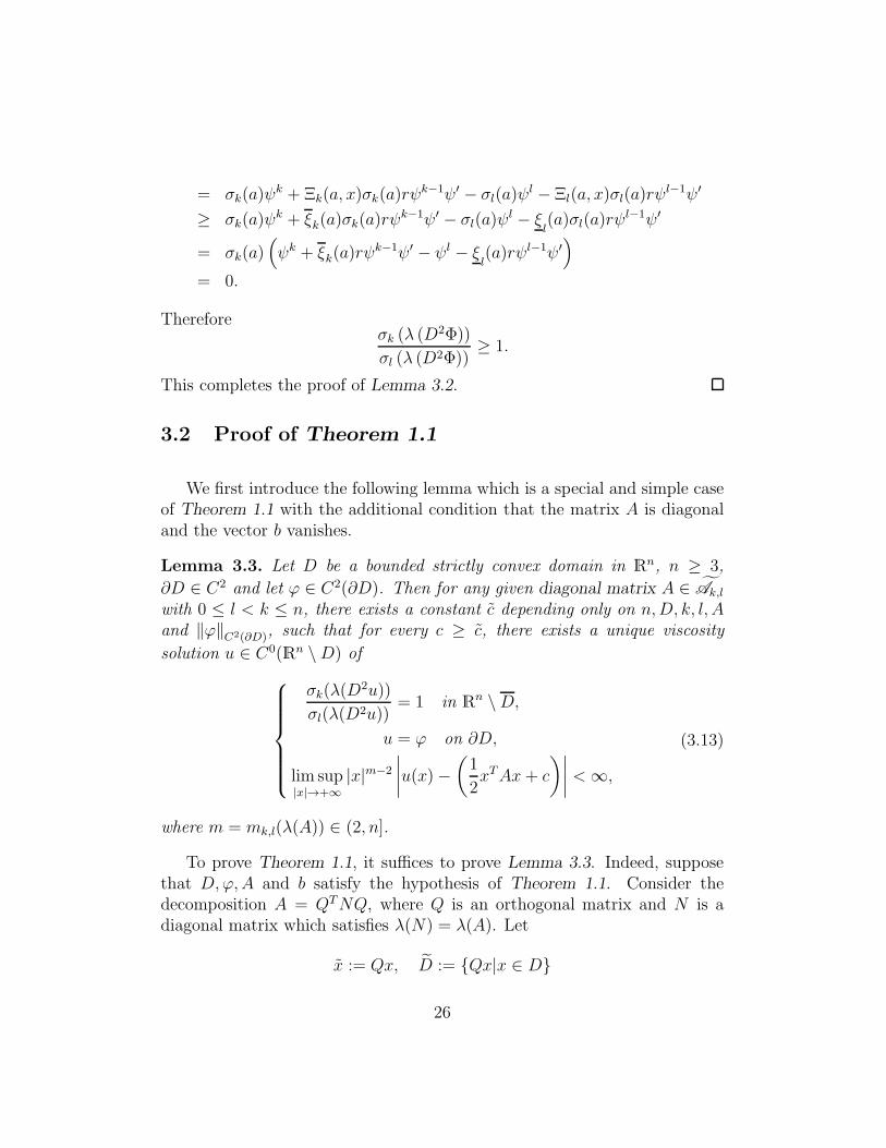
This completes the proof of Lemma 3.2.

3.2 Proof of Theorem 1.1

We first introduce the following lemma which is a special and simple caseof Theorem 1.1 with the additional condition that the matrix A is diagonaland the vector b vanishes.

Lemma 3.3. Let D be a bounded strictly convex domain in Rn, n ≥ 3,

∂D ∈ C2 and let ϕ ∈ C2(∂D). Then for any given diagonal matrix A ∈ Ak,l

with 0 ≤ l < k ≤ n, there exists a constant c depending only on n,D, k, l, Aand ‖ϕ‖C2(∂D), such that for every c ≥ c, there exists a unique viscosity

solution u ∈ C0(Rn \D) of

σk(λ(D2u))

σl(λ(D2u))= 1 in Rn \D,

u = ϕ on ∂D,

lim sup|x|→+∞

|x|m−2

∣∣∣∣u(x)−(1

2xTAx+ c

)∣∣∣∣ <∞,

(3.13)

where m = mk,l(λ(A)) ∈ (2, n].

To prove Theorem 1.1, it suffices to prove Lemma 3.3. Indeed, supposethat D,ϕ,A and b satisfy the hypothesis of Theorem 1.1. Consider thedecomposition A = QTNQ, where Q is an orthogonal matrix and N is adiagonal matrix which satisfies λ(N) = λ(A). Let

x := Qx, D := Qx|x ∈ D

26

andϕ(x) := ϕ(x)− bTx = ϕ(QT x)− bTQT x.

By Lemma 3.3, we conclude that there exists a constant c depending only onn, D, k, l, N and ‖ϕ‖C2(∂D), such that for every c ≥ c, there exists a unique

viscosity solution u ∈ C0(Rn \ D) of

σk(λ(D2u))

σl(λ(D2u))= 1 in Rn \ D,

u = ϕ on ∂D,

lim sup|x|→+∞

|x|m−2

∣∣∣∣u(x)−(1

2xTNx+ c

)∣∣∣∣ <∞,

(3.14)

where m = mk,l(λ(N)) = mk,l(λ(A)) ∈ (2, n]. Let

u(x) := u(x) + bTx = u(Qx) + bTx = u(x) + bTQT x.

We claim that u is the solution of (1.7) in Theorem 1.1. To show this, weonly need to note that

D2u(x) = QTD2u(x)Q, λ(D2u(x)

)= λ

(D2u(x)

);

u = ϕ on ∂D;

and

|x|m−2

∣∣∣∣u(x)−(1

2xTNx+ c

)∣∣∣∣

=(xTQTQx

)(m−2)/2

∣∣∣∣u(x)− bTx−(1

2xTQTNQx + c

)∣∣∣∣

= |x|m−2

∣∣∣∣u(x)−(1

2xTAx+ bTx+ c

)∣∣∣∣ .

Thus we have proved that Theorem 1.1 can be established by Lemma 3.3.

Remark 3.2. (1) We may see from the above demonstration that the lowerbound c of c in Theorem 1.1 can not be discarded generally. Indeed, forthe radial solutions of the Hessian equation σk(λ(D

2u)) = 1 in Rn \B1,[WB13, Theorem 2] states that there is no solution when c is too small.

27

(2) Unlike the Poisson equation and the Monge-Ampere equation, generally,for the Hessian quotient equation, the matrix A in Theorem 1.1 canonly be normalized to a diagonal matrix, and can not be normalized toI multiplied by some constant. This is the reason why we study thegeneralized radially symmetric solutions, rather than the radial solutions,of the original equation (1.1). See also [BLL14].

Now we use the Perron’s method to prove Lemma 3.3.

Proof of Lemma 3.3. Wemay assume without loss of generality thatE1 ⊂⊂D ⊂⊂ Er ⊂⊂ Er and a := (a1, a2, ..., an) := λ(A) with 0 < a1 ≤ a2 ≤ ... ≤an. The proof now will be divided into three steps.

Step 1. Let

η := infx∈Er\Dξ∈∂D

Qξ(x), Q(x) := supξ∈∂D

Qξ(x)

and

Φβ(x) := η +

∫ rA(x)

r

τψ(τ, β)dτ, ∀rA(x) ≥ 1, ∀β ≥ 1,

where Qξ(x) and ψ(r, β) are given by Lemma 2.3 and Lemma 3.1, respec-tively. Then we have

(1) Since Q is the supremum of a collection of smooth solutions Qξ of(1.1), it is a continuous subsolution of (1.1), i.e.,

σk(λ(D2Q))

σl(λ(D2Q))≥ 1

in Rn \D in the viscosity sense (see [Ish89, Proposition 2.2]).

(2) Q = ϕ on ∂D. To prove this we only need to show that for any ξ ∈ ∂D,Q(ξ) = ϕ(ξ). This is obvious since Qξ ≤ ϕ on D and Qξ(ξ) = ϕ(ξ),according to Remark 2.2-(1).

(3) By Lemma 3.2, Φβ is a smooth subsolution of (1.1) in Rn \D.

28

(4) Φβ ≤ ϕ on ∂D and Φβ ≤ Q on Er \D. To show them we first note thatΦβ(x) is strictly increasing with respect to rA(x) since ψ(r, β) ≥ 1 > 0by Lemma 3.1-(i). Invoking Φβ = η on ∂Er and η ≤ Q on Er \D bytheir definitions, we have Φβ ≤ η ≤ Q on Er \D. On the other hand,according to Remark 2.2-(1), we have Qξ ≤ ϕ on D which implies thatη ≤ ϕ on D. Combining these two aspects we deduce that Φβ ≤ η ≤ ϕon ∂D.

(5) Φβ(x) is strictly increasing with respect to β and

limβ→+∞

Φβ(x) = +∞, ∀rA(x) ≥ 1, (3.15)

by the definition of Φβ(x) and Lemma 3.1-(ii).

(6) As we showed in (3.11) and (3.12), for any β ≥ 1, we have

Φβ(x) = η +

∫ rA(x)

r

τψ(τ, β)dτ

= η +1

2(rA(x)

2 − r2) +

∫ rA(x)

r

τ(ψ(τ, β)− 1

)dτ

=1

2rA(x)

2 +

(η − 1

2r2 + µr(β)

)− µrA(x)(β)

=1

2rA(x)

2 + µ(β)− µrA(x)(β)

=1

2xTAx+ µ(β) +O

(|x|−m+2

)(|x| → +∞),

where we set

µ(β) := η − 1

2r2 + µr(β),

and used the fact that xTAx = O(|x|2) (|x| → +∞) since λ(A) ∈ Γ+.

Step 2. For fixed r > r, there exists β > 1 such that

min∂Er

Φβ > max∂Er

Q,

in light of (3.15). Thus we obtain

Φβ > Q on ∂Er. (3.16)

29

Letc := max

η, µ(β), c

,

where the c comes from Remark 2.2-(3), and hereafter fix c ≥ c.By Lemma 3.1 and Corollary 3.1 we deduce that

ψ(r, 1) ≡ 1 ⇒ µr(1) = 0 ⇒ µ(1) = η − 1

2r2 < η ≤ c ≤ c,

andlim

β→+∞µr(β) = +∞ ⇒ lim

β→+∞µ(β) = +∞.

On the other hand, it follows from Corollary 3.1 that µ(β) is continuous andstrictly increasing with respect to β

(which indicates that the inverse of µ(β)

exists and µ−1 is strictly increasing). Thus there exists a unique β(c) such

that µ(β(c)) = c. Then we have

Φβ(c)(x) =1

2rA(x)

2+c−µrA(x)(β(c)) =1

2xTAx+c+O

(|x|−m+2

)(|x| → +∞),

andβ(c) = µ−1(c) ≥ µ−1(c) ≥ β.

Invoking the monotonicity of Φβ with respect to β and (3.16), we obtain

Φβ(c) ≥ Φβ > Q on ∂Er. (3.17)

Note that we already know

Φβ(c) ≤ Q on Er \D,

from (4) of Step 1.

Let

u(x) :=

max

Φβ(c)(x), Q(x)

, x ∈ Er \D,

Φβ(c)(x), x ∈ Rn \ Er.

Then we have

(1) u is continuous and satisfies

σk(λ(D2u))

σl(λ(D2u))≥ 1

in Rn \D in the viscosity sense, by (1) and (3) of Step 1.

30

(2) u = Q = ϕ on ∂D, by (2) of Step 1.

(3) If rA(x) is large enough, then

u(x) = Φβ(c)(x) =1

2xTAx+ c +O

(|x|−m+2

)(|x| → +∞).

Step 3. Let

u(x) :=1

2xTAx+ c, ∀x ∈ Rn.

Then u is obviously a supersolution and

lim|x|→+∞

(u− u) (x) = 0.

To use the Perron’s method to establish Lemma 3.3, we now only needto prove that

u ≤ u in Rn \D.In fact, since

µrA(x)(β) ≥ 0, ∀x ∈ Rn \ E1, ∀β ≥ 1,

according to Corollary 3.1, we have

Φβ(c)(x) =1

2xTAx+ c− µrA(x)(β(c)) ≤

1

2xTAx+ c = u(x), ∀x ∈ Rn \D.

(3.18)(We remark that this (3.18) can also be proved by using the comparison

principle, in view of

Φβ(c) ≤ η ≤ c ≤ c ≤ u on ∂D,

andlim

|x|→+∞

(Φβ(c) − u

)(x) = 0.

)

On the other hand, for every ξ ∈ ∂D, since

Qξ(x) ≤1

2xTAx+ c ≤ 1

2xTAx+ c ≤ 1

2xTAx+ c = u(x), ∀x ∈ ∂D,

andQξ ≤ Q < Φβ(c) ≤ u on ∂Er

31

follows from (3.17) and (3.18), we obtain

Qξ ≤ u on ∂ (Er \D) .

In view ofσk(λ(D

2Qξ))

σl(λ(D2Qξ))= 1 =

σk(λ(D2u))

σl(λ(D2u))in Er \D,

we deduce from the comparison principle that

Qξ ≤ u in Er \D.

HenceQ ≤ u in Er \D. (3.19)

Combining (3.18) and (3.19), by the definition of u, we get

u ≤ u in Rn \D.

This finishes the proof of Lemma 3.3.

Remark 3.3. To prove Lemma 3.3 we have used above Lemma 2.4 andLemma 2.5 presented in Subsection 2.3. In fact, one can follow the techniquesin [CL03] (see also [DB11] [Dai11] and [LD12]) instead of Lemma 2.5 torewrite the whole proof. These two kinds of presentation look a little differentbut are essentially the same.

References

[BCGJ03] J.-G. Bao, J.-Y. Chen, B. Guan, M. Ji, Liouville property and reg-ularity of a Hessian quotient equation, Amer. J. Math. 125 (2003),301–316.

[BLL14] J.-G. Bao, H.-G. Li, Y.-Y. Li, On the exterior Dirichlet problem forHessian equations, Trans. Amer. Math. Soc. 366 (2014) 12, 6183–6200.

[Cal58] E. Calabi, Improper affine hyperspheres of convex type and a gener-alization of a theorem by K. Jorgens, Michigan Math. J. 5 (1958),105–126.

32

[Caf95] L. A. Caffarelli, Topics in PDEs: The Monge-Ampere Equation,Graduate Course, Courant Institute, New York University, 1995.

[CC95] L. A. Caffarelli, X. Cabre, Fully nonlinear elliptic equations, Col-loquium Publications 43, American Mathematical Society, Provi-dence, RI, 1995.

[CIL92] M. G. Crandall, H. Ishii, P.-L. Lions, User’s guide to viscosity so-lutions of second order partial differential equations, Bull. Amer.Math. Soc. 27 (1992), 1–67.

[CL03] L. A. Caffarelli, Y.-Y. Li, An extension to a theorem of Jorgens,Calabi, and Pogorelov, Comm. Pure Appl. Math. 56 (2003), 549–583.

[CNS85] L. A. Caffarelli, L. Nirenberg, J. Spruck, The Dirichlet problemfor nonlinear second-order elliptic equations, III. Functions of theeigenvalues of the Hessian, Acta Math. 155 (1985), 261–301.

[CWY09] J.-Y. Chen, M. Warren, Y. Yuan, A priori estimate for convexsolutions to special Lagrangian equations and its application, Comm.Pure Appl. Math. 62 (2009), 583–595.

[CY86] S.-Y. Cheng, S.-T. Yau, Complete affine hypersurfaces, I. The com-pleteness of affine metrics, Comm. Pure Appl. Math. 39 (1986),839–866.

[Dai11] L.-M. Dai, The Dirichlet problem for Hessian quotient equations inexterior domains, J. Math. Anal. Appl. 380 (2011), 87–93.

[DB11] L.-M. Dai, J.-G. Bao, On uniqueness and existence of viscosity solu-tions to Hessian equations in exterior domains, Front. Math. China6 (2011), 221–230.

[Del92] P. Delanoe, Partial decay on simple manifolds, Ann. Global Anal.Geom. 10 (1992), 3–61.

[FMM99] L. Ferrer, A. Martınez, F. Milan, An extension of a theorem byK. Jorgens and a maximum principle at infinity for parabolic affinespheres, Math. Z. 230 (1999), 471–486.

33

[FMM00] L. Ferrer, A. Martınez, F. Milan, The space of parabolic affinespheres with fixed compact boundary, Monatsh. Math. 130 (2000),19–27.

[Fu98] L. Fu, An analogue of Bernstein’s theorem, Houston J. Math. 24(1998), 415–419.

[HL82] R. Harvey, H. B. Lawson, Calibrated geometries, Acta Math. 148(1982), 47–157.

[HLP34] G. H. Hardy, J. E. Littlewood, G. Polya, Inequalities, first edi-tion, Cambridge University Press, Cambridge, 1934 (second edition,1952).

[Ish89] H. Ishii, On uniqueness and existence of viscosity solutions of fullynonlinear second-order elliptic PDEs, Comm. Pure Appl. Math. 42(1989), 15–45.

[Ivo85] N. N. Ivochkina, Solution of the Dirichlet problem for some equa-tions of Monge-Ampere type, Mat. Sb. 128 (1985), 403–415, Englishtransl. 56 (1987), 403–415.

[Jen88] R. Jensen, The maximum principle for viscosity solutions of fullynonlinear second order partial differential equations, Arch. Ration.Mech. Anal. 101 (1988), 1–27.

[Jor54] K. Jorgens, uber die Losungen der Differentialgleichung rt−s2 = 1,Math. Ann. 127 (1954), 130–134.

[JX01] J. Jost, Y.-L. Xin, Some aspects of the global geometry of entirespace-like submanifolds, Results Math. 40 (2001), 233–245.

[Kry83] N. V. Krylov, On degenerate nonlinear elliptic equations, Mat. Sb.121 (1983), 301–330, English transl. 48 (1984), 307–326.

[LL16] D.-S. Li, Z.-S. Li, On the exterior Dirichlet problem for special La-grangian equations, in preparation.

[LB14] H.-G. Li, J.-G. Bao, The exterior Dirichlet problem for fully non-linear elliptic equations related to the eigenvalues of the Hessian, J.Differential Equations 256 (2014), 2480–2501.

34

[LD12] H.-G. Li, L.-M. Dai, The exterior Dirichlet problem for Hessianquotient equations, J. Math. Anal. Appl. 393 (2012), 534–543.

[MS60] N. Meyers, J. Serrin, The exterior Dirichlet problem for second orderelliptic partial differential equations, J. Math. Mech. 9 (1960), 513–538.

[Pog72] A. V. Pogorelov, On the improper convex affine hyperspheres, Ge-ometriae Dedicata 1 (1972), No. 1, 33–46.

[Tru90] N. S. Trudinger, The Dirichlet problem for the prescribed curvatureequations, Arch. Rational Mech. Anal. 111 (1990), No. 2, 153–179.

[Tru95] N. S. Trudinger, On the Dirichlet problem for Hessian equations,Acta Math. 175 (1995), 151–164.

[TW00] N. S. Trudinger, X.-J. Wang, The Bernstein problem for affine max-imal hypersurface, Invent. Math. 140 (2000), 399–422.

[Urb90] J. I. E. Urbas, On the existence of nonclassical solutions for twoclass of fully nonlinear elliptic equations, Indiana Univ. Math. J.39 (1990), 355–382.

[WB13] C. Wang, J.-G. Bao, Necessary and sufficient conditions on exis-tence and convexity of solutions for Dirichlet problems of Hessianequations on exterior domains, Proc. Amer. Math. Soc. 141 (2013),1289–1296.

[Yuan02] Y. Yuan, A Bernstein problem for special Lagrangian equations,Invent. Math. 150 (2002), 117–125.

35