Online Generated Kick Motions for the NAOBalanced Using Inverse Dynamics

Felix Wenk1 and Thomas Rofer2

1 Universitat Bremen, Fachbereich 3 – Mathematik und Informatik,Postfach 330 440, 28334 Bremen, GermanyE-Mail: fwenk@informatik.uni-bremen.de

2 Deutsches Forschungszentrum fur Kunstliche Intelligenz,Cyber-Physical Systems, Enrique-Schmidt-Str. 5, 28359 Bremen, Germany

E-Mail: thomas.roefer@dfki.de

Abstract. One of the major tasks of playing soccer is kicking the ball.Executing such complex motions is often solved by interpolating key-frames of the entire motion or by using predefined trajectories of thelimbs of the soccer robot. In this paper we present a method to generatethe trajectory of the kick foot online and to move the rest of the robot’sbody such that it is dynamically balanced. To estimate the balance ofthe robot, its Zero-Moment Point (ZMP) is calculated from its movementusing the solution of the Inverse Dynamics. To move the ZMP, we useeither a Linear Quadratic Regulator on the local linearization of the ZMPor the Cart-Table Preview Controller and compare their performances.

1 Introduction

To play humanoid soccer, two essential motion tasks have to be carried out:walking over a soccer field and kicking the ball. Both motions have to be bothflexible and robust, i.e. the robot has to be able to walk in different directions atdifferent speeds and kick the ball in different directions with different strengths,all while maintaining its balance to prevent falling over.

To design and execute motions to kick the ball, different methods have beendeveloped. A seemingly obvious approach to motion design is to manually set upsome configurations, i.e. sets of joint angles called key-frames, which the robotshall assume during the motion, and then interpolate between these key-frameswhile the motion is executed. This quite popular method has been used to designkick motions by a number of RoboCup Standard Platform League (SPL) teamsincluding B-Human [12] and Nao Team HTWK [13].

Because it completely determines the robot’s motion, the interpolation be-tween fixed sets of joint angles precludes any reaction to changing demands orto external disturbances. Therefore, Czarnetzki et al. [3] specify key-frames ofthe motion of the robot’s limbs in Cartesian space instead of joint space. Thisleaves the movement of the robot under-determined, so the Cartesian key-frameapproach can be combined with a controller to maintain balance.

To design more flexible kick motions, Muller et al. [11] model the trajec-tories of the robot’s hands and feet in Cartesian space using piecewise Beziercurves. Depending on the position of the ball relative to the kicking robot andthe desired kick direction, the Bezier curves are modified such that the kick footactually hits the ball in the desired direction. The modification of the Beziercurves is constrained such that the resulting curve is always continuously differ-entiable, which results in a smooth trajectory. In addition, a balancing controlleris included to maintain static balance by tilting the robot such that its center ofmass (COM) stays within the support polygon, i.e. the contour of the supportfoot. To make sure the robot gets properly tilted, the angular velocity measuredby gyroscopes in the robot’s torso is used as feedback.

In this work, the approaches mentioned in this introduction are combined toa motion engine that generates and executes dynamically balanced kick motions,but neither requires prior modeling of trajectories of limbs nor needs prerecordedkey-frames to interpolate. Instead of searching the path of the kick foot to theball like Xu et al. [15], the trajectory of the kick foot is an interpolation betweena number of reference poses inferred from the ball position, the kick directionand the kick strength. The points are interpolated using a spline that is contin-uously differentiable twice so that the trajectory of the kick foot has no suddenjumps in acceleration [6]. The limbs of the robot, which are not part of the kickleg and whose motion is therefore not determined by the kick foot trajectory,are moved to maintain dynamic balance, i.e. to keep the Zero-Moment Point(ZMP) [14] within the support polygon. To achieve this, the ZMP is calculatedvia the solution of the Inverse Dynamics based on an estimate of the motionof the joints. Two different methods to move the ZMP are implemented andcompared: first a Linear Quadratic Regulator (LQR) [9, 4], which modifies thejoint angles directly using a linearization of the ZMP depending on the motionof the joints, and second a Preview Controller [10] which generates a trajectoryfor the COM depending the current and the preview of the future ZMP [8]. TheCOM trajectory is then translated to joint angles using inverse kinematics.

The rest of the paper is organized as follows. The generation of the trajectoryof the kick foot is treated in Sect. 2. Section 3 covers the motion of the robotto maintain dynamic balance. The latter includes the calculation of the balancecriterion, the ZMP, and therefore the solution of the Inverse Dynamics. Exper-iments and their results including a comparison of the two balancing methodsmake up Sect. 4. Section 5 finally concludes this work.

2 Generating the Kick Foot Motion

To generate the kick foot motion, a number of reference points have to be cal-culated. At first it has to be determined which part of the contour of the footshould hit the ball. Because the contour of the foot is round and the kick footwill not be rotated during the kick, the kick is approximately a collision betweentwo spheres. So the tangent at the contact point on the foot contour has to be

rp

b d

s1

s2

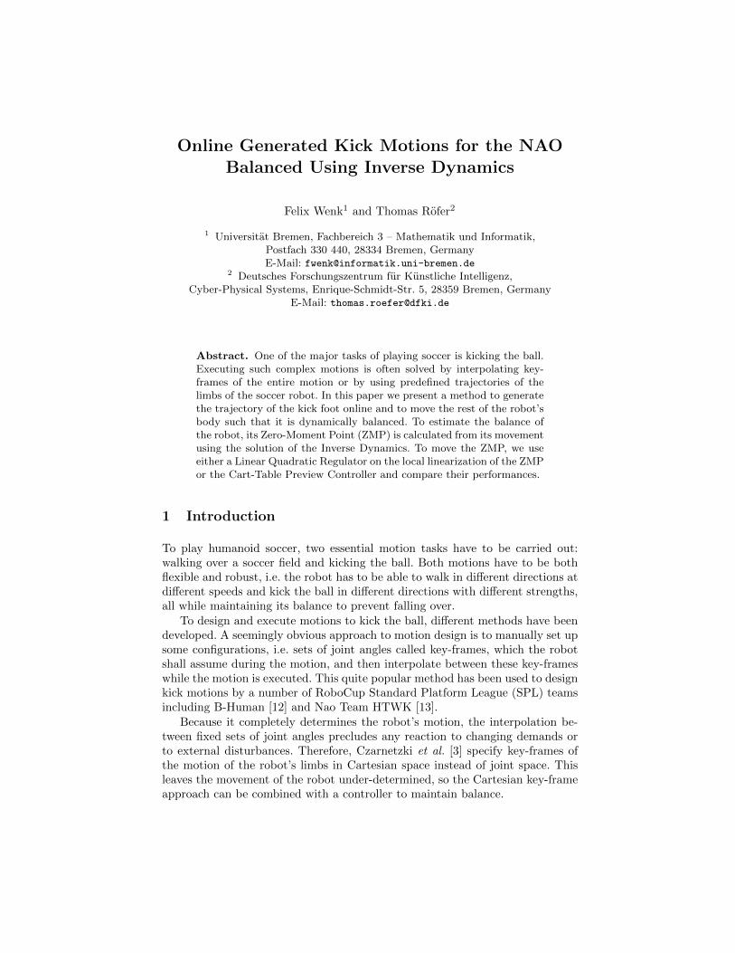
(a) (b)

Fig. 1. a) The kick foot is to collide with the ball at the point where the foot contour’stangent is orthogonal to the kick direction. b) Geometric construction of the strikeouts1 and swing s2 reference points.

orthogonal to the kick direction. To calculate the tangent, we approximate thecontour of the front of the foot with a cubic Bezier curve.

A cubic Bezier curve of dimension d is described by four control pointsp0,p1,p2,p3 ∈ IRd, which jointly determine the resulting curve

C(t) =

3∑i=0

B3i,[α,β](t) · pi with t ∈ [α, β] , α, β ∈ IR . (1)

Bni,[α,β](t) =(ni

)·(t−αβ−α

)i·(β−tβ−α

)n−1is the i-th Bernstein polynomial of degree

n defined on the interval [α, β] [6]. The derivative of such a curve is

C(t) =3

β − α·

2∑i=0

(pi+1 − pi)B2i,[α,β](t) . (2)

As shown in Fig. 1a, the ball contact point on the contour Cfoot is then

Cfoot(tbc) with Cfoot(tbc) · d = 0 , (3)

where d ∈ IR2 is the normalized kick direction vector in the plane of the soccerfield. Since the support foot (hopefully!) does not move during a kick, its coor-dinate system serves as the reference for all coordinates related to the kick foottrajectory. The resulting curve describes the trajectory of the origin of the kickfoot. Since Cfoot(tbc) is relative to the origin of the kick foot, the ball contactreference point b satisfies b + Cfoot(tbc) = pball, where pball ∈ IR2 is the ballposition on the pitch.

The points s1 ∈ IR2 and s2 ∈ IR2 to strike out and swing out the kick footare the intersections of the line in kick direction through the ball reference pointwith a circle of radius r around the pelvis joint at p ∈ IR2 of the support leg.The construction is pictured in Fig. 1b. p, s1 and s2 are all in a plane parallelto the field. The height of the plane is a parameter to be tuned by the user. r

is determined manually so that the kick foot can reach all points on the circle.If s2 gets too close to the support leg side of the pelvis or even enters it, it ispulled back on the kick direction line as pictured in Fig. 1b, so that a smallsafety margin to the support leg remains and collisions between the kick footand the support leg are avoided.

Aside from the ball position and the kick direction, the user of the kick enginealso specifies the duration T of the kick foot motion and the speed v the kickfoot should have when the ball is hit.

This information is used to determine the durations of the individual pieces ofthe curve. The curve must pass through the six points rj with 0 ≤ j < 6 in order.The i-th curve segment starts at ri, ends at ri+1 and takes the duration ∆i. Thesegment around the ball from r2 = b − λ1d to r3 = b + λ2d shall be passed in∆2 = λ1+λ2

v . It turned out that a good choice for λ1 and λ2 is if they sum up toa little more than one diameter of the ball. The speed at which to move the kickfoot back to the end position of the trajectory is set to v

4 , so the duration for

the last phase is ∆4 = 4·‖r5−r4‖v . The other durations are calculated such that

they are proportional to the square root of the length between their end pointsand sum up to T −∆2−∆4. This is also called centripetal parameterization [6].

The durations ∆i with 0 ≤ i < 5 are equivalent to a knot sequence ofa cubic B-Spline curve with the clamped end condition [6]. The clamped endcondition requires that the derivative of the curve is 0 at the ends, i.e. in thiscase B(0) = B(T ) = 0, meaning physically that the kick foot does not move.B-Spline curves are a generalization of Bezier curves. As a cubic Bezier curve, acubic B-Spline curve is a linear combination of control points dj , which are alsocalled de Boor points [6, 2].

B(u) =

L∑j=0

N3j (u)dj (4)

Nnj (u) are called the B-Spline basis functions or just B-Splines and are recur-

sively defined as

Nnj (u) =

u− uj−1uj+n−1 − uj−1

Nn−1j (u) +

uj+n − uuj+n − uj

Nn−1j+1 (u) (5)

with N0j (u) =

{1 if uj−1 ≤ u ≤ uj0 otherwise

.

L in (4) is the index of the last control point. For a B-Spline curve of degree n,this is L = K + 1 − n, where K + 1 is the number of knots. A B-Spline curveis defined over the interval [un−1, uL], i.e. in the cubic case over [u2, uL]. Eachreference point is associated with a knot. Since we want the curve to start atr0 and end at r5, this means that B(ui+2) = ri. This implies that L = 7, sothere are 8 control points and K + 1 = L + n = 10 knots in the knot sequenceu0, . . . , u9. The clamped end condition defines the knots that are not associatedto reference points to be u0 = u1 = u2 and u9 = u8 = u7. Given the durations

between the reference points and that we want the curve to be defined on theinterval [0, T ], the knots are

u2 = 0 and ui+2 = ui+2−1 +∆i−1 for 0 < i < 5 . (6)

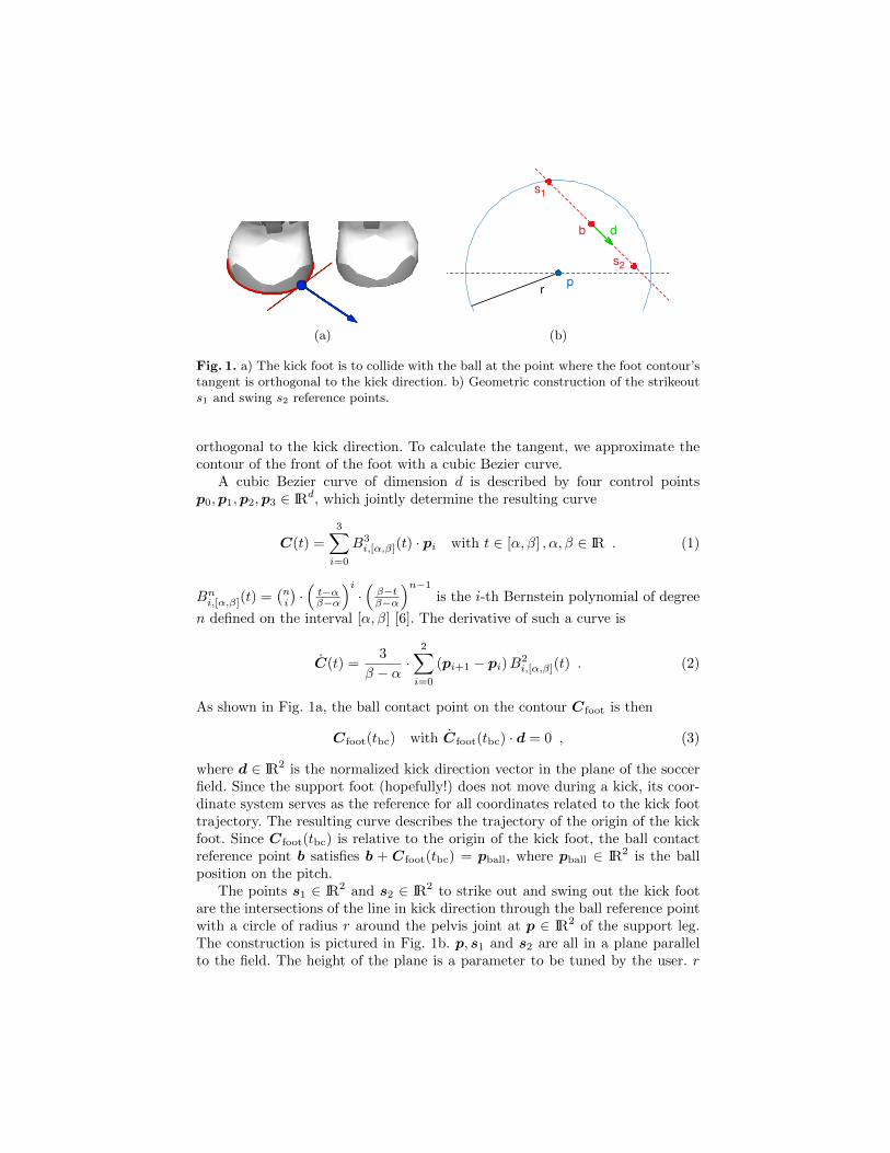
Due to the clamped end condition the first two control points collapse withthe first reference point and the last two control points collapse with the lastreference point, so d0 = d1 = r0 and d6 = d7 = r5. By inserting the associationbetween knots and reference points B(ui+2) = ri into (4) and by replacing theknown control points with the corresponding reference points, we get a system offour equations for the remaining four control points. Figure 2 shows two differentcurves calculated by using this scheme. Since the B-Spline curves are infinitelyoften continuously differentiable between the knots and n−r times continuouslydifferentiable at a knot occurring r times in the knot sequence [6], the resultingcurve is always at least 3− 1 times continuously differentiable.

Fig. 2. Trajectories (blue) of the kick foot with the corresponding de Boor points (reddots). On the left, the speed of the kick foot is too large, so that some parts of thetrajectory (red) are unreachably far away from the hip. On the right this is fixed bylowering the speed of the foot, resulting in a completely reachable trajectory.

If the speed v of the kick foot is too high relative to the kick duration T ,the segment leading up to the ball contact segment may get too long, so thatsome parts of the curve are not reachable by the kick foot. To check whetherthis is the case, we calculate the point B(umax) on that segment with themaximum (squared) distance from the pelvis joint of the kick leg and testwhether this is larger than the maximum distance allowed dmax, i.e. whetherB(umax) ·B(umax) > d2max. If this is true we define the error function

e(v) = ‖B(umax) ·B(umax)− d2max‖ (7)

by making the speed v variable and keeping all other parameters of the curveconstruction fixed. Knowing that the current v is too large, we calculate thelargest acceptable kick foot speed as v′ = argminve(v) using (7). The effect ofthis procedure is pictured in Fig. 2, where an infeasible curve with a high kickfoot speed is turned into a feasible one.

3 Dynamically Balanced Kick Foot Motion

Now that the kick foot trajectory is generated, it needs to be executed while therobot is dynamically balanced.

3.1 Balance Estimation

To determine how balanced the robot is, we estimate the difference between thecurrent ZMP p0 and a demanded ZMP p0,d. The ZMP is defined as the pointin the support polygon, i.e. the sole of the support foot, at which the (vertical)reaction force the ground exerts on the foot must act, such that all (horizontal)torques are canceled out [14]. If p0 does not exist and the then-fictional ZMPlies outside of the foot sole, the robot will begin to rotate about the edge of thesole and probably fall over eventually. With f r,z being the vertical componentof the reaction force, τ xy the total torque of the robot relative to the projectionof the support foot’s origin on the ground, n the normal vector on the groundand × denoting the cross product of two vectors, the ZMP p0 satisfies

p0 × f r,z + τ xy = 0 and therefore p0 =n× (−τ xy)

n · f r,z=

1

fr,z

τy−τx

0

. (8)

If the ZMP exists as in Fig. 3, the robot is said to be dynamically balanced.

fr,z

fr

p0oτxyτ

Fig. 3. The vertical component fr,z of the reaction force fr acts on the Zero-Momentpoint p0 to cancel out the horizontal component τxy of the total torque τ relative tothe origin of the sole of the support foot.

To calculate the ZMP, we need to know f r,z and τ xy. To infer these from

the robot motion, we estimate the angle θj , angular velocity θj and angular

acceleration θj of each joint j and solve the Inverse Dynamics problem using avariation [5] of the Recursive Newton-Euler Algorithm (RNEA) [7]. As the jointangle measurements are too noisy for simple numerical differentiation, we obtain

the estimates for θj and θj by numerically differentiating the target joint anglesinstead. Using Kalman filters [9] for each non-leg joint and one Kalman filter foreach support leg, we filter the differences ∆θj , ∆θj , and ∆θj between the actualand commanded joint motions similar to the work of Belanger [1]. These areadded to the commanded joint motions obtained by numerical differentiation.This allows us to use very small process variances in the filters, so that theestimates do not jump wildly while still having the estimates respond properlyto changes of the joint motions due to our own software.

The motions of the joints of a single leg are filtered in a combined stateinstead of using individual filters, because we use the rotation of the gyroscopein the NAO’s torso as a measurement model to correct the angular velocities ofthe joints of the support leg.

Since the support foot has no velocity and acceleration during the kick, itserves as the root of the kinematic tree, which is used by the RNEA to calculatethe torques and forces across the joints. We also assume an imaginary ’joint’with zero degrees of freedom between the ground and the support foot. Becausethe support foot does not move, the torque and force exerted on the supportfoot via the imaginary joint must be the reactions to the torque and force ofthe support foot and thus −τ and f r in (8). Since we do not need to know theforces transmitted by the real joints of the robot, we use a simplified version ofthe RNEA by Fang et al. [5], which only propagates the aggregated momentaand forces from the leaves of the tree to the root. From Fang et al. [5], we alsoimplemented taking the derivates

− ∂

∂θjτ ,− ∂

∂θjτ ,− ∂

∂θjτ ,

∂

∂θjf r,

∂

∂θjf r,

∂

∂θjf r for each joint j. (9)

Using these partial derivatives of (9), the partial derivatives of the ZMP p0 from(8) with respect to the joint motion are calculated by

∂

∂φjp0 =

[n×

(− ∂∂φjτ)xy

][n · f r,z]−

[n× (−τ )xy

] [n ·(

∂∂φjf r

)z

](n · f r,z)

2 (10)

with φj ∈{θj , θj , θj

}and j again being a joint of the robot.

p0,d is moved from its initial position between both feet on the ground to aposition within the sole of the support foot before the kick foot is moved, staysthere while the kick foot is moved, and is moved back to its initial position whenthe kick foot reached its final position.

3.2 Balancing with Linear Quadratic Regulation

We implemented a balancer by directly modifying the joint angles of the supportleg. To control the bearing of the robot’s torso, both the pitch joints of hip andankle as well as the roll joints of hip and ankle are coupled by a factor β, so thatif the pitch pair is modified by ∆θ′pitch, the hip joint of the pair will be modified

by ∆θhippitch = ∆θ′pitch and the ankle joint by ∆θanklepitch = β∆θ′pitch. The rollpair is analogous. With these joint pairs, the change of the ZMP is determinedby applying the chain rule using (10):

∂

∂φ′pitchp0 =

∂

∂φhippitchp0 + β · ∂

∂φanklepitchp0 with φ ∈ {θ, θ, θ} (11)

∂∂φ′

rollp0 is analogous.

We use (11) to construct a linear model to be used in a discrete-time, finite-horizon LQR [4]. If the robot was perfectly balanced, the ZMP p0 would coincidewith the demanded ZMP p0,d and the error e = p0 − p0,d would be zero. As-suming the demanded ZMP is constant, the linearization of the error over thetime interval between time Tt and Tt+1 with respect to the motions of the jointpairs is et+1 = et +∆e with

∆e = θ′roll

a1︷ ︸︸ ︷∂p0∂θ′roll

∆T +θ′roll

a2︷ ︸︸ ︷(∂p0∂θ′roll

1

2(∆T )2 +

∂p0

∂θ′roll∆T

)

+...θ′roll

b1︷ ︸︸ ︷(∂p0∂θ′roll

1

6(∆T )3 +

∂p0

∂θ′roll

1

2(∆T )2

∂p0

∂θ′roll∆T

)

+ θ′pitch

a3︷ ︸︸ ︷∂p0∂θ′pitch

∆T +θ′pitch

a4︷ ︸︸ ︷(∂p0∂θ′pitch

1

2(∆T )2 +

∂p0

∂θ′pitch∆T

)

+...θ′pitch

b2︷ ︸︸ ︷(∂p0∂θ′pitch

1

6(∆T )3 +

∂p0

∂θ′pitch

1

2(∆T )2

∂p0

∂θ′pitch∆T

), (12)

and ∆T = Tt+1 − Tt. This leads to the linear model xt+1 = Axt +But with

x =[e θ′roll θ′roll θ′pitch θ′pitch

]>u =

[...θ′roll

...θ′pitch

]>(13)

and

A =

1 0 a1,x a2,x a3,x a4,x0 1 a1,y a2,y a3,y a4,y0 0 1 ∆T 0 00 0 0 1 0 00 0 0 0 1 ∆T0 0 0 0 0 1

B =

b1,x b2,xb1,y b1,y

12 (∆T )2 0∆T 00 1

2 (∆T )2

0 ∆T

. (14)

With this model, the controls to be applied at time Tt are

ut = −(R+B>PkB

)−1B>PkAxt (15)

with

Pk = Q+A>Pk−1A−A>Pk−1B(R+B>Pk−1B

)−1B>Pk−1A , (16)

where P0 = Q, k is the horizon parameter, and Q and P are the diagonal,positive-definite matrices of the quadratic cost function C(x,u) = x>Qx +u>Ru.

We calculate the error et and the linearization of the ZMP in each executioncycle. We also keep track of θ′t, θ

′t and θ′t. From that, we build the model of (13)

and (14) and compute ut, which is the rate of change of the acceleration andwhich is constant until the next motion cycle. The next angles to be set for thehip and ankle joints are computed from θ′t+1 = θ′t+∆Tθ

′t+

12 (∆T )2θ′t+

16 (∆T )3

...θ′t

according to factor β of the joint pairing. The remaining joints of the supportleg are not changed.

To determine the angles of the kick leg, we calculate the pose of the torsousing forward kinematics, evaluate the kick foot trajectory to the new kick footpose, calculate the kick foot pose relative to the torso and use inverse kinematicsto solve for the angles of the kick leg joints.

3.3 Balancing with a Cart-Table Controller

In addition to the LQR we implemented the Cart-Table controller by Kajita etal. [8]. Instead of a linearization of the ZMP, we use a truly linear model and usean extension of a linear-quadratic controller [10], which responds more quickly tochanges of the demanded ZMP, because it also considers the N future demandsof the ZMP instead of only the currently demanded ZMP.

According to the Cart-Table model, the ZMP depends on the motion of theCOM c. With the 2-dimensional COM restricted to a plane of height cz, the2-dimensional ZMP p0 on the ground is

p0 = c− czgc . (17)

With the ZMP, which is calculated using the inverse dynamics method explainedabove, and a preview series of ZMPs that will be demanded, we calculate thecontrol output

...c , the jerk of the COM. With an initial position the COM this

effectively defines a trajectory for the COM. Using the kick foot pose from theevaluation of the kick foot trajectory, we implemented a simple numerical methodto move the robot’s torso relative to the support foot, such that the COM ismoved to the position demanded by the controller and the kick foot to the poserelative to the support foot as demanded by the kick foot trajectory.

The downside of the Cart-Table model is that it only works at a constantCOM height, which has to be approached before the actual balancing can start.Also, the effects of the angular motion of the robot around the COM are notmodeled. But the advantages outweigh the downsides. As we will see in Sec. 4,the ZMP as modeled by the Cart-Table model is not too different from the ZMPcalculated using the inverse dynamics. The computation is also much faster,because the gain matrices of the controller, including a Riccati equation such as(16), can be calculated once in advance and then repeatedly used while balancing.

-40

-20

0

20

40

60

80

0 1000 2000 3000 4000 5000 6000

zm

p [

mm

]

t [ms]

demandZMP

-40

-20

0

20

40

60

80

0 500 1000 1500 2000 2500 3000 3500

zm

p [

mm

]

t [ms]

demandZMP

Cart ZMP

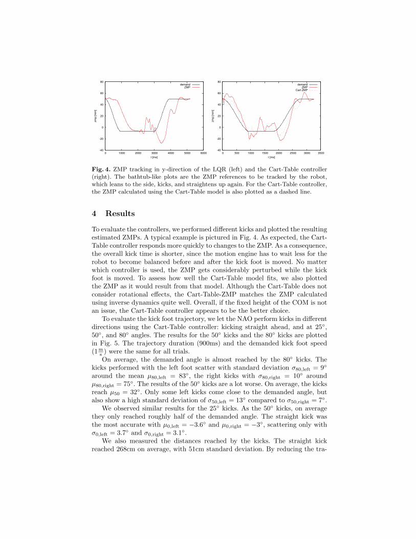
Fig. 4. ZMP tracking in y-direction of the LQR (left) and the Cart-Table controller(right). The bathtub-like plots are the ZMP references to be tracked by the robot,which leans to the side, kicks, and straightens up again. For the Cart-Table controller,the ZMP calculated using the Cart-Table model is also plotted as a dashed line.

4 Results

To evaluate the controllers, we performed different kicks and plotted the resultingestimated ZMPs. A typical example is pictured in Fig. 4. As expected, the Cart-Table controller responds more quickly to changes to the ZMP. As a consequence,the overall kick time is shorter, since the motion engine has to wait less for therobot to become balanced before and after the kick foot is moved. No matterwhich controller is used, the ZMP gets considerably perturbed while the kickfoot is moved. To assess how well the Cart-Table model fits, we also plottedthe ZMP as it would result from that model. Although the Cart-Table does notconsider rotational effects, the Cart-Table-ZMP matches the ZMP calculatedusing inverse dynamics quite well. Overall, if the fixed height of the COM is notan issue, the Cart-Table controller appears to be the better choice.

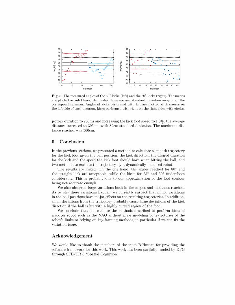
To evaluate the kick foot trajectory, we let the NAO perform kicks in differentdirections using the Cart-Table controller: kicking straight ahead, and at 25◦,50◦, and 80◦ angles. The results for the 50◦ kicks and the 80◦ kicks are plottedin Fig. 5. The trajectory duration (900ms) and the demanded kick foot speed(1m

s ) were the same for all trials.On average, the demanded angle is almost reached by the 80◦ kicks. The

kicks performed with the left foot scatter with standard deviation σ80,left = 9◦

around the mean µ80,left = 83◦, the right kicks with σ80,right = 10◦ aroundµ80,right = 75◦. The results of the 50◦ kicks are a lot worse. On average, the kicksreach µ50 = 32◦. Only some left kicks come close to the demanded angle, butalso show a high standard deviation of σ50,left = 13◦ compared to σ50,right = 7◦.

We observed similar results for the 25◦ kicks. As the 50◦ kicks, on averagethey only reached roughly half of the demanded angle. The straight kick wasthe most accurate with µ0,left = −3.6◦ and µ0,right = −3◦, scattering only withσ0,left = 3.7◦ and σ0,right = 3.1◦.

We also measured the distances reached by the kicks. The straight kickreached 268cm on average, with 51cm standard deviation. By reducing the tra-

5

10

15

20

25

30

35

40

45

50

55

0 10 20 30 40 50

angle

[deg]

trial index

55

60

65

70

75

80

85

90

95

100

0 5 10 15 20 25 30 35 40 45

angle

[deg]

trial index

Fig. 5. The measured angles of the 50◦ kicks (left) and the 80◦ kicks (right). The meansare plotted as solid lines, the dashed lines are one standard deviation away from thecorresponding mean. Angles of kicks performed with left are plotted with crosses onthe left side of each diagram, kicks performed with right on the right sides with circles.

jectory duration to 750ms and increasing the kick foot speed to 1.3ms , the average

distance increased to 395cm, with 82cm standard deviation. The maximum dis-tance reached was 560cm.

5 Conclusion

In the previous sections, we presented a method to calculate a smooth trajectoryfor the kick foot given the ball position, the kick direction, the desired durationfor the kick and the speed the kick foot should have when hitting the ball, andtwo methods to execute the trajectory by a dynamically balanced robot.

The results are mixed. On the one hand, the angles reached for 80◦ andthe straight kick are acceptable, while the kicks for 25◦ and 50◦ undershootconsiderably. This is probably due to our approximation of the foot contourbeing not accurate enough.

We also observed large variations both in the angles and distances reached.As to why these variations happen, we currently suspect that minor variationsin the ball positions have major effects on the resulting trajectories. In addition,small deviations from the trajectory probably cause large deviations of the kickdirection if the ball is hit with a highly curved region of the foot.

We conclude that one can use the methods described to perform kicks ofa soccer robot such as the NAO without prior modeling of trajectories of therobot’s limbs or relying on key-framing methods, in particular if we can fix thevariation issue.

Acknowledgement

We would like to thank the members of the team B-Human for providing thesoftware framework for this work. This work has been partially funded by DFGthrough SFB/TR 8 “Spatial Cognition”.

References

1. Belanger, P.: Estimation of angular velocity and acceleration from shaft encodermeasurements. In: Robotics and Automation, 1992. Proceedings., 1992 IEEE In-ternational Conference on. pp. 585 –592 vol.1 (May 1992)

2. de Boor, C.: On calculating with B-splines. Journal of Approximation The-ory 6(1), 50 – 62 (1972), http://www.sciencedirect.com/science/article/pii/0021904572900809

3. Czarnetzki, S., Kerner, S., Klagges, D.: Combining key frame based motion designwith controlled movement execution. In: Baltes, J., Lagoudakis, M., Naruse, T.,Ghidary, S. (eds.) RoboCup 2009: Robot Soccer World Cup XIII, Lecture Notesin Computer Science, vol. 5949, pp. 58–68. Springer Berlin Heidelberg (2010)

4. Doya, K.: Bayesian Brain: Probabilistic Aproaches to Neural Coding. Computa-tional Neuroscience Series, MIT Press (2007)

5. Fang, A.C., Pollard, N.S.: Efficient synthesis of physically valid human motion.ACM Trans. Graph. 22(3), 417–426 (Jul 2003), http://doi.acm.org/10.1145/

882262.882286

6. Farin, G.: Curves and Surfaces for CAGD: A Practical Guide. The Morgan Kauf-mann Series in Computer Graphics and Geometric Modeling (2002)

7. Featherstone, R.: Rigid Body Dynamics Algorithms. Springer (2008)8. Kajita, S., Kanehiro, F., Kaneko, K., Fujiwara, K., Harada, K., Yokoi, K.,

Hirukawa, H.: Biped walking pattern generation by using preview control of zero-moment point. In: Robotics and Automation, 2003. Proceedings. ICRA ’03. IEEEInternational Conference on. vol. 2, pp. 1620 – 1626 vol.2 (Sept 2003)

9. Kalman, R.E.: A new approach to linear filtering and prediction problems. Trans-actions of the ASME–Journal of Basic Engineering 82, 35–45 (1960), online:http://www.cs.unc.edu/~welch/kalman/media/pdf/Kalman1960.pdf

10. Katayama, T., Ohki, T., Inoue, T., Kato, T.: Design of an optimal controller fora discrete-time system subject to previewable demand. International Journal ofControl 41(3), 677–699 (1985)

11. Muller, J., Laue, T., Rofer, T.: Kicking a ball – modeling complex dynamic motionsfor humanoid robots. In: del Solar, J.R., Chown, E., Ploeger, P.G. (eds.) RoboCup2010: Robot Soccer World Cup XIV. Lecture Notes in Artificial Intelligence, vol.6556, pp. 109–120. Springer (2011)

12. Rofer, T., Laue, T., Muller, J., Bosche, O., Burchardt, A., Damrose, E., Gillmann,K., Graf, C., de Haas, T.J., Hartl, A., Rieskamp, A., Schreck, A., Sieverdingbeck, I.,Worch, J.H.: B-Human Team Report and Code Release 2009 (2009), only availableonline: http://www.b-human.de/file_download/26/bhuman09_coderelease.pdf

13. Tilgner, R., Reinhardt, T., Borkmann, D., Kalbitz, T., Seering, S., Fritzsche, R.,Vitz, C., Unger, S., Eckermann, S., Muller, H., Bellersen, M., Engel, M., Wunsch,M.: Team research report 2011 Nao-Team HTWK Leipzig (2011), available online:http://robocup.imn.htwk-leipzig.de/documents/report2011.pdf

14. Vukobratovic, M., Borovac, B.: Zero-moment point — thirty five years of its life.International Journal of Humanoid Robotics 01(01), 157–173 (2004), http://www.worldscientific.com/doi/abs/10.1142/S0219843604000083

15. Xu, Y., Mellmann, H.: Adaptive motion control: Dynamic kick for a humanoidrobot. In: Dillmann, R., Beyerer, J., Hanebeck, U., Schultz, T. (eds.) KI 2010:Advances in Artificial Intelligence, Lecture Notes in Computer Science, vol. 6359,pp. 392–399. Springer Berlin Heidelberg (2010)