Technical report from Automatic Control at Linköpings universitet

Online Estimation of Ship’s Mass andCenter of Mass Using InertialMeasurements

Jonas Linder?, Martin Enqvist?, Thor I. Fossen†, Tor ArneJohansen†, Fredrik Gustafsson?

Division of Automatic ControlE-mail: jonas.linder@liu.se, maren@isy.liu.se,thor.fossen@ntnu.no, tor.arne.johansen@itk.ntnu.no,fredrik@isy.liu.se

13th March 2015

Report no.: LiTH-ISY-R-3081Submitted to the 10th IFAC Conference on Manoeuvring and Controlof Marine Craft

Address:?Department of Electrical EngineeringLinköpings universitetSE-581 83 Linköping, Sweden†Centre for Autonomous Marine Operations and Systems (AMOS),Department of Engineering CyberneticsNorwegian University of Science and TechnologyNO-7491 Trondheim, Norway

WWW: http://www.control.isy.liu.se

AUTOMATIC CONTROLREGLERTEKNIK

LINKÖPINGS UNIVERSITET

Technical reports from the Automatic Control group in Linköping are available fromhttp://www.control.isy.liu.se/publications.

AbstractA ship’s roll dynamics is sensitive to the mass and mass distribution.Changes in these physical properties might introduce unpredictable behav-ior of the ship and a worst-case scenario is that the ship will capsize. Inthis paper, a recently proposed approach for online estimation of mass andcenter of mass is validated using experimental data. The experiments wereperformed using a scale model of a ship in a wave basin. The data wascollected in free run experiments where the rudder angle was recorded andthe ship’s motion was measured using an inertial measurement unit. Themotion measurements are used in conjunction with a model of the roll dy-namics to estimate the desired properties. The estimator uses the rudderangle measurements together with an instrumental variable method to mit-igate the influence of disturbances. The experimental study shows that theproperties can be estimated with quite good accuracy but that variance androbustness properties can be improved further.

Keywords: modelling, identification, operational safety, inertial measure-ment unit, identifiability, centre of mass, physical models, accelerometers,gyroscopes, marine systems

1 IntroductionIn marine vessels, mathematical models are nowadays commonly used to in-crease performance or accuracy. A good model is essential, for instance, inmodel-based control where a poor model will affect the performance negatively(Skogestad and Postlethwaite, 2005), or in decision supp-ort systems where anerror in the model might result in bad advice. Ships have time-dependent prop-erties and by estimating these online, a higher model accuracy can be achieved.One example is the mass of a container ship being changed due to loading ofcontainers. The dynamic behavior of the ship is affected by these propertiesand a large variation of certain properties might be safety critical.

A ship’s roll dynamics is very sensitive to changes in the loading conditionsand a worst-case scenario is that the ship will capsize (Fossen, 2011; Tannuriet al., 2003). Iseki and Terada (2001) study the problem of estimating the direc-tional wave spectrum from ship motion. The wave spectrum can then be used tosimulate a ship’s response over time, to apply control or to suggest appropriateactions. This is basically an inverse problem and the result is dependent on theship’s mass. Inaccurate knowledge of the ship’s mass, and thus of the model,might lead to an inaccurate wave spectrum, which in the end might lead to poorperformance if the wave spectrum is used in the earlier mentioned control ordecision support systems.

Perez (2005) presents methods for ship roll stabilization or ship roll reductionsystems using model-based control. The model used in the approach is a linearmaneuvering model where the parameters are assumed to be known. The effectsof model errors are not investigated, but due to changes in the ship roll dynamicsshown in, for instance, Fossen (2011) and Tannuri et al. (2003), it seems likelythat a significant change in mass will affect the ship dynamics and that onlineestimation of the mass would make it possible to increase the performance ofthe controller.

In most mechanical systems, the mass is actually one of the properties thatinfluence the dynamics the most. If the forces acting on the system are notknown, it is difficult to uniquely determine the mass with motion data onlysince large forces acting on a heavy system cannot be distinguished from smallforces acting on a light system. This ambiguity can be overcome with specialexperiments where the forces acting on the system are known, or by introducingsensors that can measure the forces. However, introducing special sensors orexperiments is in many cases intractable or too expensive.

Online mass estimation for vehicles has been considered in especially auto-motive applications, see for instance, Fathy et al. (2008). However, for a ship,there are additional challenges that are not present in ground vehicles due tothe complex interaction with the water. For example, there are strong couplingsbetween the ship’s degrees of freedom and the motion of the ship is strongly af-fected by the environmental disturbances.

An approach to mitigate the influence of the environmental disturbancesusing an instrumental variable (IV) method and the rudder angle was proposedin Linder et al. (2014b) and Linder et al. (2014a). A simplified model of theroll dynamics was used and it was assumed that only motion data from aninertial measurement unit (IMU) together with the rudder angle were available.In Linder et al. (2015), an extended model was derived from well-establishedresults in literature to also consider the strong couplings in ships.

1

This paper presents an experimental study of online estimation of a ship’smass and center of mass using the recently proposed approach derived in Linderet al. (2015) with data recorded from a scale ship operated in a basin. The datawas collected under moderate sea conditions in free run experiments where thescale model was controlled manually using a joystick. The goals of the study areto validate the model and method using real data, and to evaluate the properties,such as the accuracy, of the estimator. Furthermore, to investigate the influencesfrom disturbances, the IV estimator is compared with a least-squares estimator.

The outline of this paper is: In Section 2, the model used in the approachis introduced. In Section 3, the model is discretized, identifiability issues arediscussed and an IV estimator is suggested to estimate the model. Sections 4and 5 introduce the experimental setup and the data. Finally, the results arepresented and discussed in Section 6 and conclusions are given in Section 7.

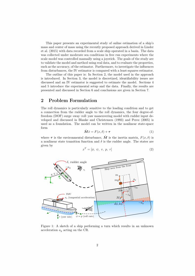
2 Problem FormulationThe roll dynamics is particularly sensitive to the loading condition and to geta connection from the rudder angle to the roll dynamics, the four degree-of-freedom (DOF) surge–sway–roll–yaw maneuvering model with rudder input de-veloped and discussed in Blanke and Christensen (1993) and Perez (2005) isused as a foundation. The model can be written in the nonlinear state-spaceform

M x = F (x, δ) + τ (1)

where τ is the environmental disturbance, M is the inertia matrix, F (x, δ) isa nonlinear state transition function and δ is the rudder angle. The states aregiven by

xT = [φ, ψ, v, p, r] (2)

m

mg

�zs

�zg

�

Mg

d�, k�

M�zm

as

�ay

Ship seen from the front

r (yaw rate)

as (tangential acceleration)

� = p (roll rate)

IMU

�, rudder angle

xn

yn

⌧t

xbyb

�ay

X,Y,

Figure 1: A sketch of a ship performing a turn which results in an unknownacceleration ay acting on the CR.

2

where φ is the roll angle and ψ is the yaw angle expressed in a Earth-fixedcoordinate system which is assumed to be inertial. Furthermore, v is the linearsurge speed, p is the angular velocity about the roll axis and r is the angularvelocity about the yaw axis expressed in a body-fixed coordinate system.

Since the actual forces acting on the ship are unknown and we instead workwith measurement of the motion, we will estimate the change in mass and changein center of mass (CM). The total mass of the ships is split into a nominal massM and a load mass m with CMs given by zg and zm, respectively, see Figure 1for a sketch.

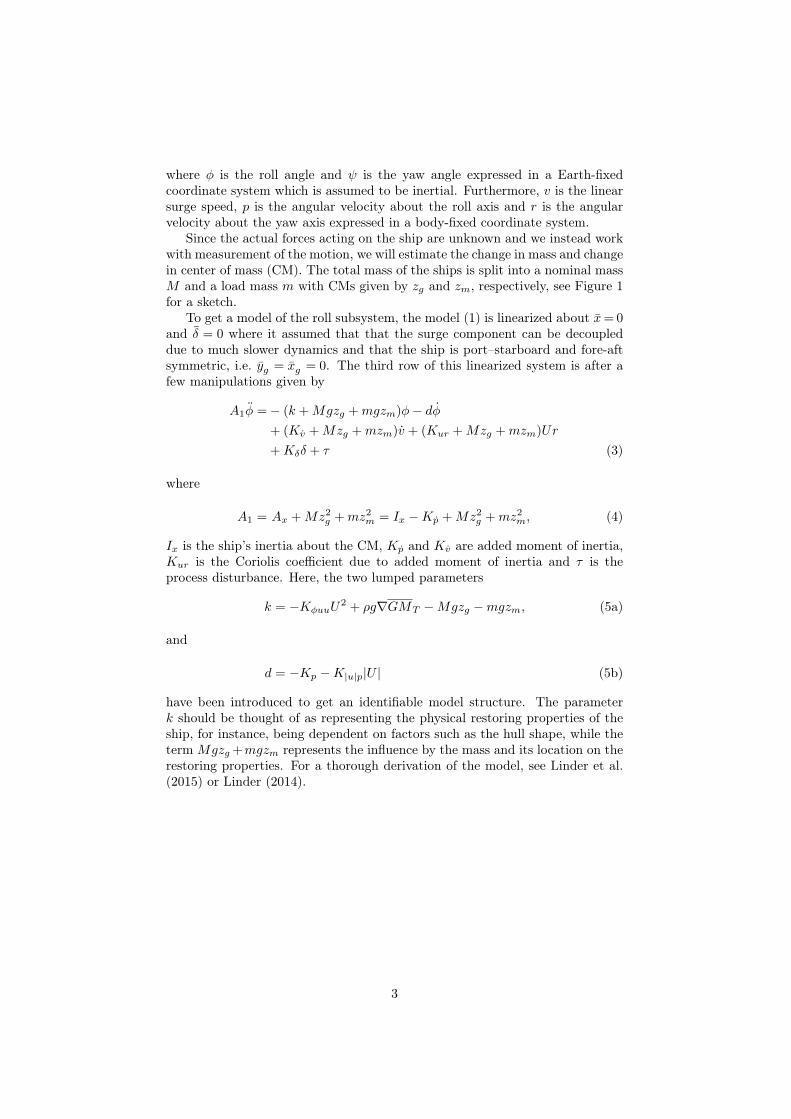
To get a model of the roll subsystem, the model (1) is linearized about x= 0and δ = 0 where it assumed that that the surge component can be decoupleddue to much slower dynamics and that the ship is port–starboard and fore-aftsymmetric, i.e. yg = xg = 0. The third row of this linearized system is after afew manipulations given by

A1φ =− (k +Mgzg +mgzm)φ− dφ+ (Kv +Mzg +mzm)v + (Kur +Mzg +mzm)Ur

+Kδδ + τ (3)

where

A1 = Ax +Mz2g +mz2

m = Ix −Kp +Mz2g +mz2

m, (4)

Ix is the ship’s inertia about the CM, Kp and Kv are added moment of inertia,Kur is the Coriolis coefficient due to added moment of inertia and τ is theprocess disturbance. Here, the two lumped parameters

k = −KφuuU2 + ρg∇GMT −Mgzg −mgzm, (5a)

and

d = −Kp −K|u|p|U | (5b)

have been introduced to get an identifiable model structure. The parameterk should be thought of as representing the physical restoring properties of theship, for instance, being dependent on factors such as the hull shape, while theterm Mgzg +mgzm represents the influence by the mass and its location on therestoring properties. For a thorough derivation of the model, see Linder et al.(2015) or Linder (2014).

3

2.1 Sensors – Intertial Measurement Unit (IMU)The ship’s motion is assumed to be observed with an IMU and the IMU’sposition can be seen in Figure 1. The IMU measurements are

y1,t = pt + b1,t + e1,t = φt + b1,t + e1,t (6a)y2,t = as,t + b2,t + e2,t (6b)y3,t = −rt + b3,t + e3,t (6c)

(6d)

where pt = φt is the sampled system’s angular velocity about the roll axis, as,tis the tangential acceleration after sampling, rt is the sampled system’s angularvelocity about the yaw axis, bi,t, i = 1, 2, 3, are sensor biases and ei,t, i = 1, 2, 3,are measurement noise. Assuming that the roll angle φ is small, the accelerationsensed by the IMU is

as = zsφ+ gφ− ay, (7)

where −zs is the distance from the center of rotation (CR) to the origin of theIMU coordinate system. The first term is the contribution from the angularacceleration, the second term is due to gravity and the third term is the acceler-ation of the CR in the xy–plane in the earth-fixed frame. Note that the identityp = φ is not valid in general and only holds due to the assumption of small rollangles.

2.2 A Limited Sensor ApproachWith v, r, δ and τ as inputs, the model (3) is a mass–spring–damper model.The issue is that v is unknown but an alternative model can be formed byeliminating v. The key to this elimination is the known relation between themeasured tangential acceleration as defined in (7), the acceleration ay and thesignal v (Linder et al., 2015). The acceleration ay of the ship in the Earth-fixedxy–plane has two parts, firstly a contribution from the sway motion and secondlydue to the angular velocity about the yaw axis. The total sway acceleration isgiven by

ay = v + Ur (8)

which means that v is indirectly measured by the tangential acceleration as.Combining (8) with (7), solving for v and substituting it into (3) give

A2φ =− (k −Kvg)φ− dφ− (Kv +Mzg +mzm)as + (Kur −Kv)Ur

+Kδδ + τ

(9)

where

A2 = Ax +Mzg(zg − zs) +mzm(zm − zs)−Kvzs (10)

If the surge speed U is assumed to be constant, this model can be furthersimplified by introducing the lumped parameter Kr = (Kur−Kv)U which givesthe model

A2φ =− (k −Kvg)φ− dφ− (Kv +Mzg +mzm)as +Krr +Kδδ + τ (11)

4

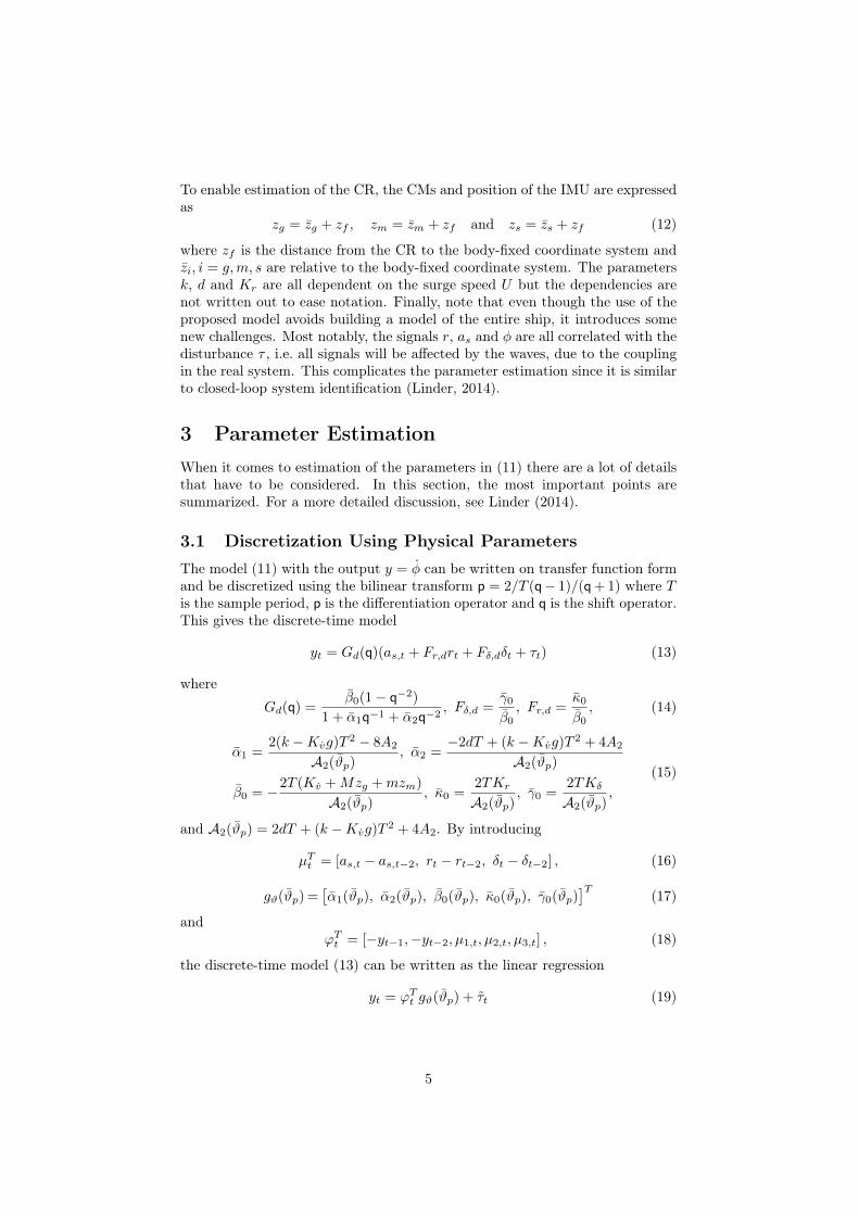
To enable estimation of the CR, the CMs and position of the IMU are expressedas

zg = zg + zf , zm = zm + zf and zs = zs + zf (12)

where zf is the distance from the CR to the body-fixed coordinate system andzi, i = g,m, s are relative to the body-fixed coordinate system. The parametersk, d and Kr are all dependent on the surge speed U but the dependencies arenot written out to ease notation. Finally, note that even though the use of theproposed model avoids building a model of the entire ship, it introduces somenew challenges. Most notably, the signals r, as and φ are all correlated with thedisturbance τ , i.e. all signals will be affected by the waves, due to the couplingin the real system. This complicates the parameter estimation since it is similarto closed-loop system identification (Linder, 2014).

3 Parameter EstimationWhen it comes to estimation of the parameters in (11) there are a lot of detailsthat have to be considered. In this section, the most important points aresummarized. For a more detailed discussion, see Linder (2014).

3.1 Discretization Using Physical ParametersThe model (11) with the output y = φ can be written on transfer function formand be discretized using the bilinear transform p = 2/T (q− 1)/(q+ 1) where Tis the sample period, p is the differentiation operator and q is the shift operator.This gives the discrete-time model

yt = Gd(q)(as,t + Fr,drt + Fδ,dδt + τt) (13)

where

Gd(q) =β0(1− q−2)

1 + α1q−1 + α2q−2, Fδ,d =

γ0

β0, Fr,d =

κ0

β0, (14)

α1 =2(k −Kvg)T 2 − 8A2

A2(ϑp), α2 =

−2dT + (k −Kvg)T 2 + 4A2

A2(ϑp)

β0 = −2T (Kv +Mzg +mzm)

A2(ϑp), κ0 =

2TKr

A2(ϑp), γ0 =

2TKδ

A2(ϑp),

(15)

and A2(ϑp) = 2dT + (k −Kvg)T 2 + 4A2. By introducing

µTt = [as,t − as,t−2, rt − rt−2, δt − δt−2] , (16)

gϑ(ϑp) =[α1(ϑp), α2(ϑp), β0(ϑp), κ0(ϑp), γ0(ϑp)

]T (17)

andϕTt = [−yt−1,−yt−2, µ1,t, µ2,t, µ3,t] , (18)

the discrete-time model (13) can be written as the linear regression

yt = ϕTt gϑ(ϑp) + τt (19)

5

3.2 Identifiability Issues – Using Multiple DatasetsThe subject of uniquely determining the parameters in a chosen model structureis both connected to the model structure considered and the informativity ofthe data set used for identification (Bazanella et al., 2010). Assuming that gand zs are known, the model (11) with φ as an output is not identifiable withrespect to the parameters

ϑTp =[M, zg, k, Ax, d, Kr, Kv, Kδ, zf , m, zm

], (20)

using a single dataset due to over-parameterization. To overcome this identi-fiability issue, more information has to be introduced. In this work, the extrainformation is introduced through the datasets

Zn = (yt, ut, δt)Nn+tnt=1+tn

and Zc = (yt, ut, δt)Nc+tct=1+tc

(21)

which are called the nominal and calibration dataset, respectively. The nominaldataset is collected with a known nominal mass M with the CM zg while thecalibration dataset has a different known mass and the total CM expressed usingthe load mass m=mc with the CM zm= zc. Then during normal operation, theloaded dataset

Zl = (yt, ut, δt)Nl+tlt=1+tl

(22)

is collected and all parameters can be estimated simultaneously using the jointmodel

yt = ϕTt θ(ϑp) + τ t (23)

where yt = [ynt , yct , y

lt]T ,

θ(ϑp)=[gTϑ (ϑnp ), gTϑ (ϑcp), g

Tϑ (ϑlp)

]T, ϕt=

ϕnt 0 00 ϕct 00 0 ϕlt

, (24)

ϑp = [

ϑp,1 (known)︷ ︸︸ ︷M, zg, mc, zc,

ϑp,2 (unknown)︷ ︸︸ ︷k, Ax, d, Kr, Kv, Kδ, zf , m, zm]

T, (25)

ϑnp = ϑp|m=zm=0, ϑcp = ϑp|m=mczm=zc , ϑ

lp = ϑp (26)

and the subscripts i = n, c, l correspond to the nominal, calibration and loadeddatasets, respectively. Note that the starting times ti, i = n, c, l are used toemphasize that these datasets are not collected at the same time. For moredetails, see Linder et al. (2015) or Linder (2014).

6

3.3 The Instrumental Variable EstimatorThere are two terms contributing to the output of (23), one containing infor-mation about the interesting input-output relation and the second containinga contribution from disturbances. An instrumental variable (IV) method usesinstruments to extract the interesting information from the data. In principle,the interesting information is estimated by requiring that the sample covariancebetween the instruments and the prediction error should be zero (Söderströmand Stoica, 1989). A good instrument should in this case be correlated with themotion induced by the rudder but be uncorrelated with the process disturbanceτ , the sensor biases bi,t, and the measurement noises ei,t. This idea is imple-mented using a version of the extended IV method, where the parameters arefound by computing

ϑ = argminϑ‖YN − ΦNθ(ϑ)‖2 , (27)

ΦN=[ζ1. . .ζN ]

ϕT1...ϕTN

, YN=[ζ1. . .ζN ]

y,1...y,N

, ζt=ζntNn

0 0

0ζctNc

0

0 0ζltNl

(28)

and ‖x‖2 =xTx. The superscript i = n, c, l, corresponds to the datasets definedin Section 3.2 and for brevity, i = n, c, l is not explicitly written at all places inthis section. See, for instance, Söderström and Stoica (1989) or Ljung (1999)for more details on the instrumental variable method.

The method presented in this section is based on the method of Gilson et al.(2006) where the parameters are estimated in an iterative scheme. In eachiteration, the instruments are created by simulating the inputs and the outputsfrom the rudder angle by using the latest parameter estimates and the iterationsare terminated when the parameters have converged.

In the jth iteration, firstly, ˆϑi,jp are estimated using the vectors of instrumentsfrom the j−1th iteration. To create the instruments, the output and inputs of(13) are simulated with δit as input, which gives the signals

yi,jt = Gi,jδy,d(q)δit, ai,js,t = Gi,jδas,d(q)δit and r

i,0t = Gi,0δr,d(q)δit (29)

and the instrument vectors are created according to

ζi,jt =[yi,jt . . . yi,jt−ny+1, µ

i,j1,t . . . µ

i,j1,t−nas+1,

µi,j2,t . . . µi,j2,t−nr+1, µ

i3,t . . . µ

i3,t−nδ+1

]T (30)

where the constants nk, k = y, as, r, δ, are the number of time lags (includingthe non-delay signal) included in ζi,jt , for instance, nδ = 0 means that µ3,t is notincluded in ζi,jt . In the initializing (0th) iteration, the transfer functions of (29)are blackbox models estimated from data. In the refining steps, the transferfunctions of (29) are given by

Gi,jδy,d =Gi,jd

1−Gi,jd Fi,jy,d

[(F i,jr,d − U)Gi,0δr,d + F i,jδ,d

], (31)

Gi,jδas,d =Gi,jd

1−Gi,jd Fi,jy,d

[F i,jδ,d + F i,jr,dG

i,0δr,d

]+

UGi,0δr,d

1− F i,jy,dGi,jd

, (32)

where Gi,0δr,d are the blackbox models estimated from data in the initialization

step and the dependencies on q and ˆϑi,jp have been dropped for brevity.

7

3.4 Summary of the ApproachIn this work, the ship’s current mass and CM are found by online estimationof the deviation from the nominal mass M and CM zg. This is necessary sincethe approach uses motion data from an IMU. The drawback for not knowingthe forces acting on the ship is the requirement of a priori information. Thenecessary information is:

• A nominal dataset collected with a known mass M and CM zg

• A calibration dataset collected with known change in mass mc and changein CM zc

• The position of the IMU zs

Finally, the loaded dataset is collected during normal operation and the changein mass m and change in CM zm can be estimated simultaneously with theother parameters according to Section 3.3. Note that the required positionzi, i = g, c, s are in relation to the body-fixed coordinate system chosen by theuser and that the CR is estimated.

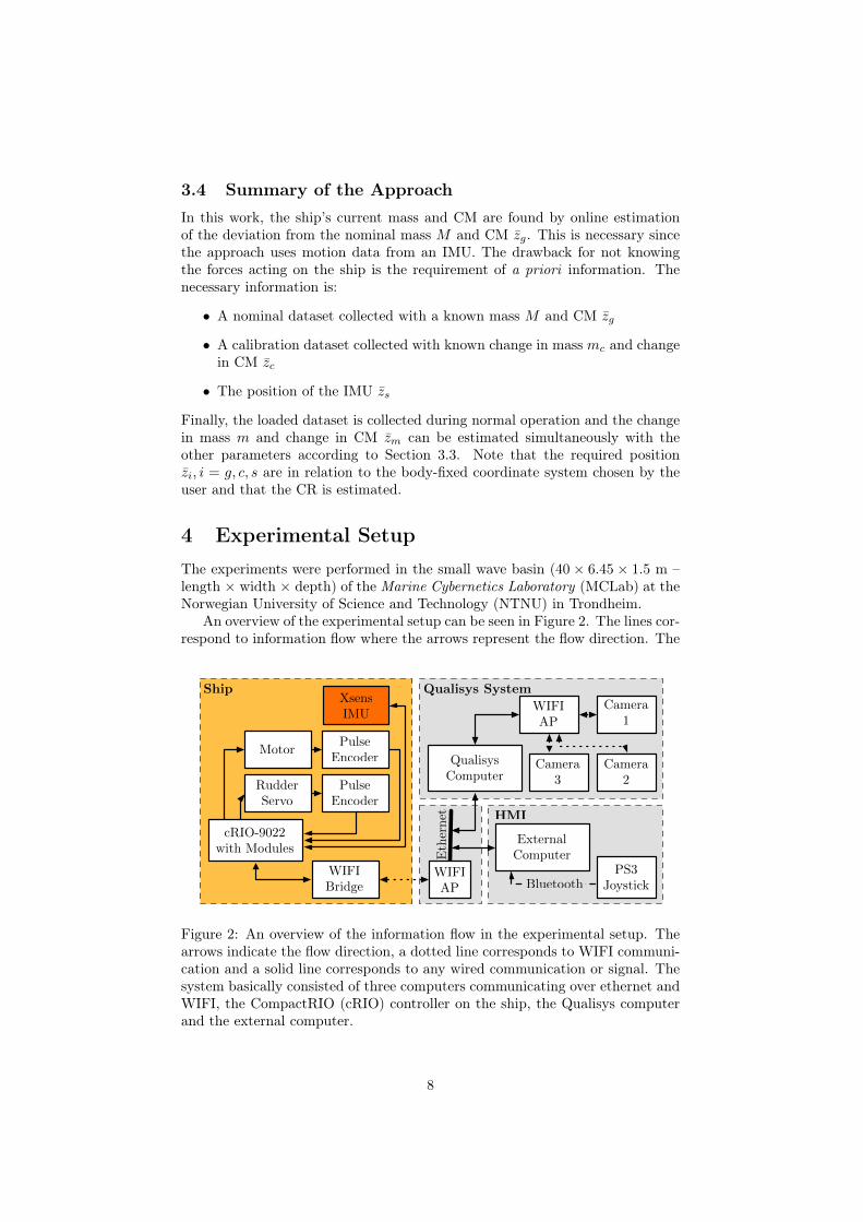
4 Experimental SetupThe experiments were performed in the small wave basin (40 × 6.45 × 1.5 m –length × width × depth) of the Marine Cybernetics Laboratory (MCLab) at theNorwegian University of Science and Technology (NTNU) in Trondheim.

An overview of the experimental setup can be seen in Figure 2. The lines cor-respond to information flow where the arrows represent the flow direction. The

Eth

ernet

Qualisys System

QualisysComputer

WIFIAP

Camera1

Camera2

Camera3

Ship

HMI

ExternalComputer

BluetoothPS3

JoystickWIFIAP

PulseEncoder

Motor

PulseEncoder

RudderServo

WIFIBridge

cRIO-9022with Modules

XsensIMU

Figure 2: An overview of the information flow in the experimental setup. Thearrows indicate the flow direction, a dotted line corresponds to WIFI communi-cation and a solid line corresponds to any wired communication or signal. Thesystem basically consisted of three computers communicating over ethernet andWIFI, the CompactRIO (cRIO) controller on the ship, the Qualisys computerand the external computer.

8

Table 1: “Our Lass II” in scale 1 : 24. Model parameters originating from Thys(2013).

Parameter Model UnitLength between perpendiculars Lpp 0.8 mLength at the waterline Lw 0.85 mBeam B 0.3 mDraft at COG D 0.144 mDraft fore Df 0.144 mDraft aft Da 0.144 mDisplacement ∆ 22.04 kgLCG from midship 0.125 mKG 0.146 mGMT 0.018 mRadius of Gyration in Roll Kxx/B 0.337 mRadius of Gyration in Pitch Kyy/L 0.272 mRadius of Gyration in Yaw Kzz/L 0.272 m

dashed line corresponds to bluetooth communication, dotted lines correspondto WIFI communication and solid lines correspond to any wired communica-tion or signal. The system had three major components, the ship, the Qualisysreal-time positioning system and the human-machine interface.

The scale model, hereafter called the ship, was a model of a fishing vesselcalled “Our Lass II” that is roughly 20 m long, see Figure 3. The ship was inscale 1 : 24 and the known physical quantities are listed in Table 1. The shiphad a cRIO Controller that ran the LabVIEW Real-Time operating system andcommunicated via a WIFI bridge to the external computer that ran LabVIEW.The ship had its own propulsion and steering that were controlled through theonboard cRIO controller. The cRIO controller collected data from the threeonboard sensors, an IMU, measuring angular velocities and linear accelerations,and two pulse encoders that were measuring the RPM of the motor and thesteering angle, respectively. The IMU was an Xsens MTi-G that was equippedwith a three-axes gyro and a three-axes accelerometer and it was mounted un-derneath the black box seen on top of the ship in Figure 3.

As can be seen in Figure 3, the ship is close to square in shape, which meantthat for small changes in the roll angle, the wetted surface area should notchange much. This implies that the restoring torque will be close to linear for agiven forward speed (Journée and Massie, 2001). The position of the load waschosen to be on top of the black box covering the IMU. Since the distance fromthe CR (> 20 cm) was large, the weights had quite a big impact on the rolldynamics and stability of the ship. In the lower right picture of Figure 3, a loadmass of 2 kg was added to the ship and with this mass, it was barely stable,which resulted in a large constant roll angle. Due to this, the load masses werechosen to be 0.200 and 0.400 kg. These correspond to an increase of 0.91% and1.81% in the total mass, respectively.

The external computer was used as a human-machine interface, plotting theship’s current status, logging data and taking commands from a joystick tocontrol the ship.

9

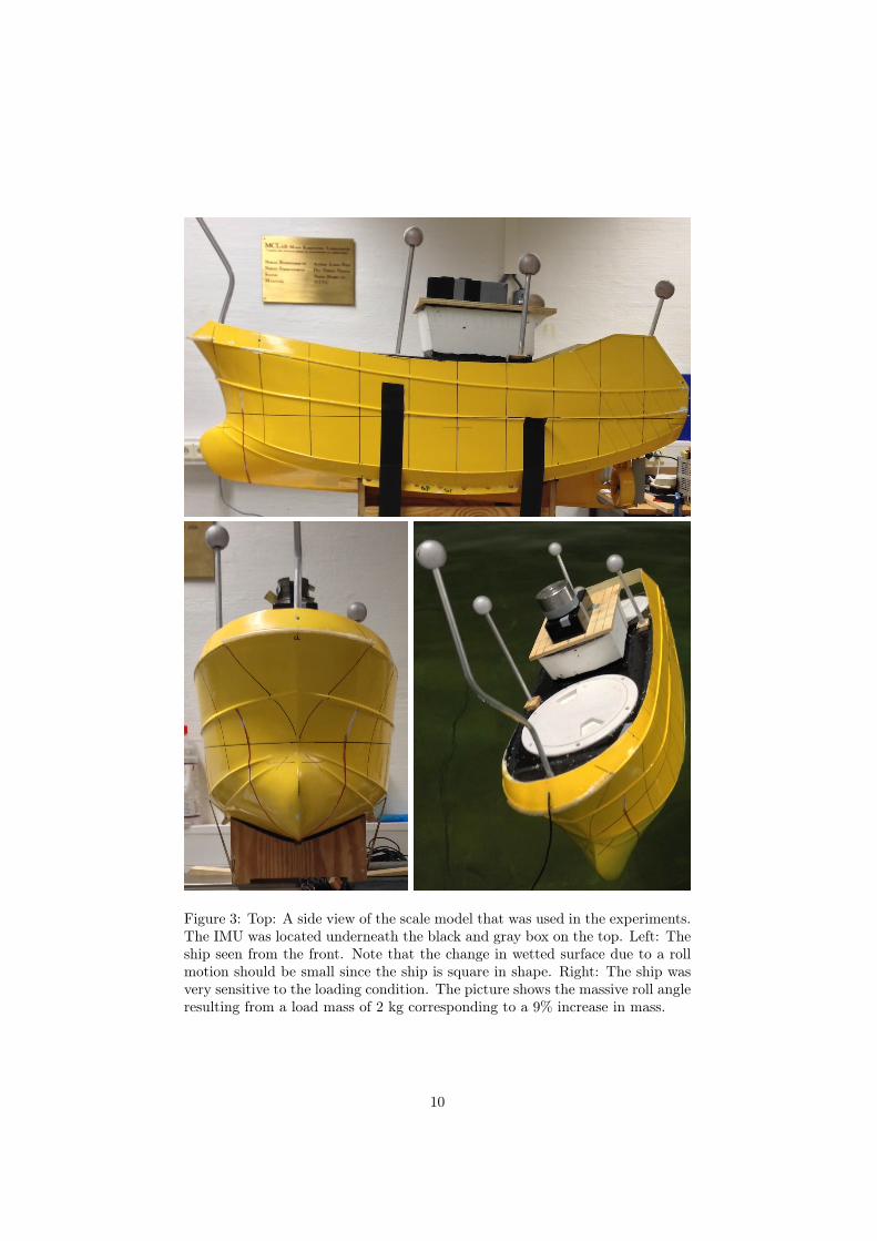
Figure 3: Top: A side view of the scale model that was used in the experiments.The IMU was located underneath the black and gray box on the top. Left: Theship seen from the front. Note that the change in wetted surface due to a rollmotion should be small since the ship is square in shape. Right: The ship wasvery sensitive to the loading condition. The picture shows the massive roll angleresulting from a load mass of 2 kg corresponding to a 9% increase in mass.

10

Table 2: A summary of the different cases.

Nominal Calibration LoadedCase 1 Nominal – 1 0.200 kg – 2 0.200 kg – 3Case 2 Nominal – 1 0.200 kg – 3 0.400 kg – 4Case 3 Nominal – 1 0.200 kg – 2 0.400 kg – 4

5 Datasets, Instruments, Noise Models and Ini-tial Values

The data was collected in free run experiments where the ship was untetheredand running by its own power. The propeller speed was kept constant and theship was manually controlled with the joystick. The runs did not follow anyparticular trajectory and both short and long turns were performed while asmuch as possible of the basin was utilized. Several datasets were recorded for 0,0.200 and 0.400 kg loads. In this paper, four datasets were used, one nominalset, two sets with 0.200 kg load mass and one with 0.400 kg load mass. Thedatasets were combined into three different cases according to Table 2. Thedatasets were sampled at 100 Hz, filtered through an FIR equiripple low-passfilter of order 20 with a cut-off frequency of 0.5 Hz and down-sampled to 50Hzresulting in a data length roughly between 1 800–3 300 samples per dataset. Asan example, the filtered nominal dataset can be seen in Figure 4.

The acceleration of gravity g and the position zs of the IMU in relation to thebody-fixed coordinate system were both assumed to be known. Furthermore,the initial conditions were in all cases assumed to be

ϑp,2 = [k, Ax, d, Kr, Kv, Kδ, zf , m, zm]T

= [9, 0.5, 0.1, −0.4, 1, −0.4, −0.018, 0, 0]T

(33)

In all iterations, the instruments (30) were created using the constants ny=16,nas =16, nr=16 and nδ=2 for each dataset. The experiments were performedwithout using the wave maker but reflections of the bow waves on the walls ofthe basin were observed. This corresponds to sea states 1 and 2 (rippled andsmooth waves) (Fossen, 2011).

6 ResultsThe instrumental variable method described in Section 3.3 was applied to eachcase in Table 2 and the results can be seen in Table 3. Note that the estimatedparameters were roughly the same in all three cases. As expected, Case 1 hadthe best results of all the cases in Table 2, probably since the calibration datasetwas similar to the loaded dataset, i.e. having the same mass and position. Theestimated mass was less than 1 g away from the true value and the CM locationhad an error of less than 4 mm. Cases 2 and 3 were more realistic cases in a sensethat the masses and the centers of gravity were different between the calibrationand loaded datasets. The largest relative error in the mass estimation was 16.6% which corresponds to 66.5 g or 0.3 % of the total mass of the ship.

11

−12 −11 −10 −9 −8 −7 −6 −5 −4 −3 −2 −1 0

−2

−1

0

1

2

−0.2

0

0.2

GyroX

−1

0

1

2

AccY

−0.6

−0.4

−0.2

0

0.2

GyroZ

−20

0

20

40

Rudder

0 10 20 30 40 50 60

350

355

360

365

370

RPM

−12 −11 −10 −9 −8 −7 −6 −5 −4 −3 −2 −1 0

−2

−1

0

1

2

−0.2

0

0.2

GyroX

−1

0

1

2

AccY

−0.6

−0.4

−0.2

0

0.2

GyroZ

−20

0

20

40

Rudder

0 10 20 30 40 50 60

350

355

360

365

370

RPM

−12 −11 −10 −9 −8 −7 −6 −5 −4 −3 −2 −1 0

−2

−1

0

1

2

−0.2

0

0.2

GyroX

−1

0

1

2

AccY

−0.6

−0.4

−0.2

0

0.2

GyroZ

−20

0

20

40

Rudder

0 10 20 30 40 50 60

350

355

360

365

370

RPM

−12 −11 −10 −9 −8 −7 −6 −5 −4 −3 −2 −1 0

−2

−1

0

1

2

−0.2

0

0.2

GyroX

−1

0

1

2

AccY

−0.6

−0.4

−0.2

0

0.2

GyroZ

−20

0

20

40

Rudder

0 10 20 30 40 50 60

350

355

360

365

370

RPM

−12 −11 −10 −9 −8 −7 −6 −5 −4 −3 −2 −1 0

−2

−1

0

1

2

−0.2

0

0.2

GyroX

−1

0

1

2

AccY

−0.6

−0.4

−0.2

0

0.2

GyroZ

−20

0

20

40

Rudder

0 10 20 30 40 50 60

350

355

360

365

370

RPM

Position[m]

Gyro x[rad/s]

Acc. as[m/s2]

Gyro z[rad/s]

Rudder[deg]Figure 4: The nominal data after filtering. The dashed red and green lines

correspond to the end of Case 1(a) and the start of Case 1(b), respectively.

10 20 30 40 50 600

0.2

0.4

0.6

0.8

1

Figure 5: Red: The normalized residuals for the nominal dataset. Gray: Thescaled absolute value of the rudder angle. The area between the rudder angleand the x–axis is filled to make the plot easier to read. Note that there arespikes at almost all the turn entries, which indicates that the model was notcapturing all the dynamics. The magnitudes of these spikes are around 10 timeslarger than the average residual.

12

Table 3: Estimation results for IV estimator on the cases in Table 2. P: param-eters, T: true values, I: initial values and E: the relative error. Here, the rowsstarting with 1,2,3,a and b correspond to the cases discussed in Section 6.

P Ax d k −Kδ −Kr Kv −zf m −zmT – – – – – – – 0.2000 0.2560I0.5000 0.1000 9.0000 0.4000 0.4000 1.0000 0.0180 0.0000 0.000010.1583 0.2685 9.0057 0.4822 2.0100 0.9607 0.0294 0.1997 0.2529E – – – – – – – 0.1338 1.2120%20.1566 0.2668 9.0067 0.4433 1.9911 0.9408 0.0293 0.3690 0.2426E – – – – – – – 7.7532 9.4842%30.1571 0.2675 9.0021 0.4383 1.9995 0.9516 0.0294 0.3335 0.2671E – – – – – – – 16.631 0.3286%a0.1552 0.2411 8.9986 0.4821 2.0227 0.9376 0.0294 0.1629 0.2977E – – – – – – – 18.557 16.271%b0.2234 0.4395 8.9967 0.5042 2.3138 1.0350 0.0246 0.3005 0.1951E – – – – – – – 50.259 23.776%

To test the variation of the IV estimator the datasets of Case 1 were split intotwo cases. Case 1(a) roughly corresponded to the first half of the datasets andCase 1(b) roughly corresponded to the last half of the datasets. As an example,the end of the nominal datasets of Case 1(a) is indicated as the dashed red linein Figure 4. In the same way, the start of the nominal dataset of Case 1(b) isindicated as the dashed green line in Figure 4. In Case 1(a), the data lengthswere 1576, 901 and 1276 samples after decimation for the nominal, calibrationand loaded datasets, respectively. For Case 1(b), the corresponding numberswere 1701, 1026 and 1401. The estimation results can be seen with the indicesA and B in Table 3. The maximum relative error, 54 % was quite large, however,it corresponds to less than 1 % of the total mass of the ship. Also, note thatthere might be a finite data effect since the datasets are quite short. Cases2 and 3 had the same nominal and loaded datasets but different calibrationdatasets which was another indication that the variation was acceptable for theIV estimator. In Figure 5 the normalized residuals are plotted together with thescaled absolute value of the rudder angle. The figure shows clear deterministiccomponents in the residuals with large spikes at the turn entries which indicatesthat there was unmodeled dynamics.

Note that no pre-processing, except for the lowpass-filtering, has been per-formed on the data. A side affect of using the IV method is that the biasesin the measurements, in addition to the process disturbance and measurementnoises, are automatically taken care of. The disturbances acting on the data,i.e. the sensor biases bi,t, i = 1, 2, 3, the process disturbance τ and measure-ment noises ei,t, i = 1, 2, 3, are quite important to consider and will introduce abias in the estimator if they are neglected. To get an indication of the impor-tance of the disturbances, the constrained least squares estimator, i.e. settingζit =ϕit, i = n, c, l, was used to compute the estimate and the result can be seenin Table 4. There is quite a significant difference compared to the IV estima-tor which performed better in all cases. Note that a constant heel angle, i.e.a that the mean of the roll angle is non-zero, only will be visible through thegravity-term in (7) and that this “bias” will be treated in the same way as a

13

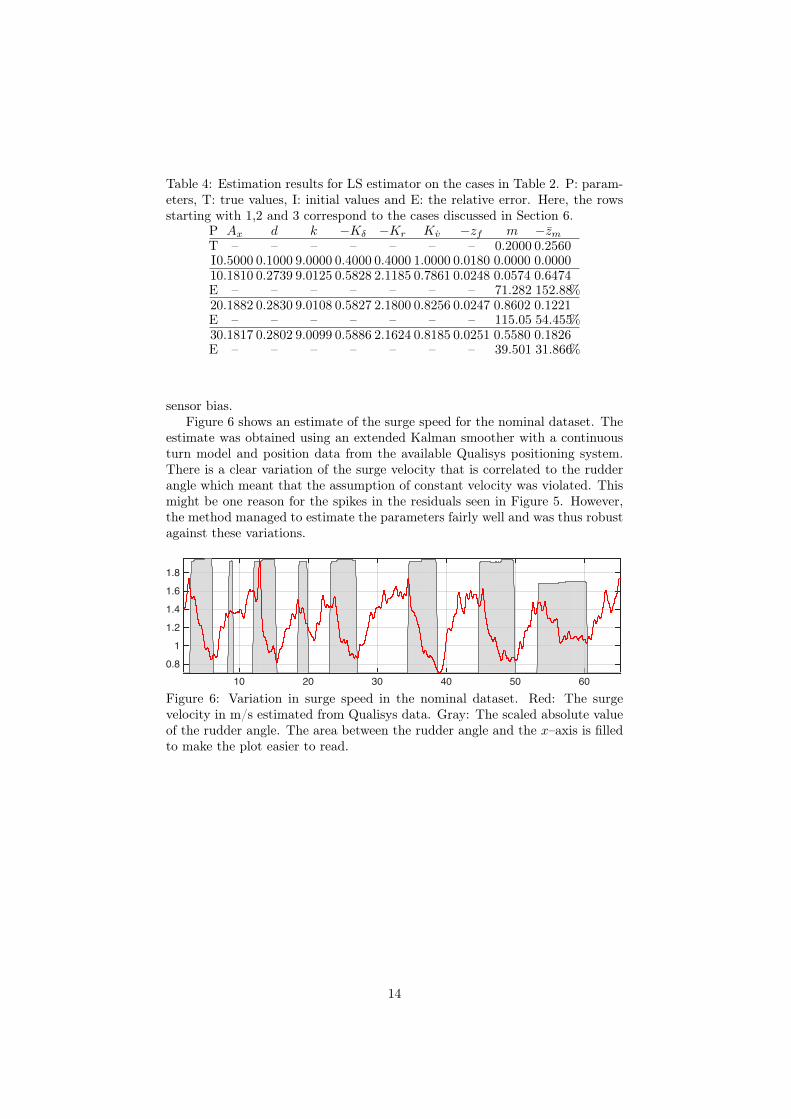
Table 4: Estimation results for LS estimator on the cases in Table 2. P: param-eters, T: true values, I: initial values and E: the relative error. Here, the rowsstarting with 1,2 and 3 correspond to the cases discussed in Section 6.

P Ax d k −Kδ −Kr Kv −zf m −zmT – – – – – – – 0.2000 0.2560I0.5000 0.1000 9.0000 0.4000 0.4000 1.0000 0.0180 0.0000 0.000010.1810 0.2739 9.0125 0.5828 2.1185 0.7861 0.0248 0.0574 0.6474E – – – – – – – 71.282 152.88%20.1882 0.2830 9.0108 0.5827 2.1800 0.8256 0.0247 0.8602 0.1221E – – – – – – – 115.05 54.455%30.1817 0.2802 9.0099 0.5886 2.1624 0.8185 0.0251 0.5580 0.1826E – – – – – – – 39.501 31.866%

sensor bias.Figure 6 shows an estimate of the surge speed for the nominal dataset. The

estimate was obtained using an extended Kalman smoother with a continuousturn model and position data from the available Qualisys positioning system.There is a clear variation of the surge velocity that is correlated to the rudderangle which meant that the assumption of constant velocity was violated. Thismight be one reason for the spikes in the residuals seen in Figure 5. However,the method managed to estimate the parameters fairly well and was thus robustagainst these variations.

10 20 30 40 50 600.8

1

1.2

1.4

1.6

1.8

Figure 6: Variation in surge speed in the nominal dataset. Red: The surgevelocity in m/s estimated from Qualisys data. Gray: The scaled absolute valueof the rudder angle. The area between the rudder angle and the x–axis is filledto make the plot easier to read.

14

7 Conclusions and future workIn this paper, online estimation of a ship’s mass and center of mass have beeninvestigated using data collected from a scale ship and a model of the shipsroll dynamics together with measurements from an inertial measurement unit.To mitigate impact of the disturbances, sensor biases and measurement noises,an iterative instrumental variable estimator was applied to the data with goodresults.

The residuals indicate a possibility for improved modeling. Future workincludes analysis of the residuals to improve the performance of the estimator.Furthermore, it would be interesting to apply the method to data from full-scaletest. In full-scale, the measured signals will be of the same magnitude as thescale model since acceleration does not scale, i.e an IMU in the same position onthe ship will sense the same acceleration as the scale model and angular velocitieswill scale like n−0.5 where n is the length scale factor. There are two big issuesthat need to be addressed in a full-scale test. Firstly, the parameters will beof different magnitude which might introduce numerical issues in the estimator.Secondly, the excitation level in the scale test were large to ensure informativityin the data and the question is if smaller excitations will significantly degradethe performance of the estimator. Since real-time estimates may not be neededall the time in an operational setting, one may incorporate logic to disable theestimator if low levels of excitation are degrading the quality of the estimates.

AcknowledgmentsThis work has been supported by the Vinnova Industry Excellence Center LINK-SIC and by the Research Council of Norway through the Centers of Excellencefunding scheme, number 223254 - Centre for Autonomous Marine Operationsand Systems (AMOS). The authors would like to thank Torgeir Wahl for hisinvaluable support during the wave basin tests.

ReferencesAlexandre Sanfelice Bazanella, Michel Gevers, and Ljubiša Miškovic. Closed-loop identification of MIMO systems: A new look at identifiability and ex-periment design. European Journal of Control, 16(3):228–239, 2010. ISSN0947-3580.

Mogens Blanke and Anders C Christensen. Rudder-roll damping autopilot ro-bustness to sway-yaw-roll couplings. In Proceedings of the 10th Ship ControlSystems Symposium, Ottawa, Canada, 1993.

H.K. Fathy, Dongsoo Kang, and J.L. Stein. Online vehicle mass estimationusing recursive least squares and supervisory data extraction. In AmericanControl Conference, 2008, pages 1842–1848, June 2008.

T. I. Fossen. Handbook of Marine Craft Hydrodynamics and Motion Control.Wiley, 2011. ISBN 9781119991496.

15

Marion Gilson, Hugues Garnier, Peter JW Young, Paul Van den Hof, et al. Arefined IV method for closed-loop system identification. In Proceedings of the14th IFAC Symposium on System Identification, pages 903–908, Newcastle,Australia, 2006.

T. Iseki and D. Terada. Bayesian estimation of directional wave spectra forship guidance system. In Proceedings of the International Offshore and PolarEngineering Conference, volume 4, pages 577–582, 2001.

J. M. J. Journée and W. W. Massie. Offshore Hydromechanics, 2001. Lec-ture notes on offshore hydromechanics for Offshore Technology students, codeOT4620.

Jonas Linder. Graybox Modelling of Ships Using Indirect Input Measurements.Linköping Studies in Science and Technology. Thesis 1681. 2014.

Jonas Linder, Martin Enqvist, and Fredrik Gustafsson. A closed-loop instru-mental variable approach to mass and center of mass estimation using IMUdata. In Proceedings of the 53rd IEEE Conference on Decision & Control,Los Angeles, CA, USA, December 2014a.

Jonas Linder, Martin Enqvist, Fredrik Gustafsson, and Johan Sjöberg. Identifi-ability of physical parameters in systems with limited sensors. In Proceedingsof the 19th IFAC World Congress, Cape Town, South Africa, August 2014b.

Jonas Linder, Martin Enqvist, Thor I. Fossen, and Tor Arne Johansen. Mod-eling for IMU-based Online Estimation of Ship’s Mass and Center of Mass.Technical Report 3082, Linköping University, The Institute of Technology,2015.

L. Ljung. System Identification: Theory for the User (2nd Edition). PrenticeHall, 1999. ISBN 0136566952.

T. Perez. Ship Motion Control: Course Keeping and Roll Stabilisation Us-ing Rudder and Fins. Advances in Industrial Control Series. Springer-VerlagLondon Limited, 2005. ISBN 9781846281570.

S. Skogestad and I. Postlethwaite. Multivariable Feedback Control: Analysis andDesign. Wiley, 2005. ISBN 9780470011676.

T.S. Söderström and P.G. Stoica. System Identification. Prentice Hall Interna-tional Series In Systems And Control Engineering. Prentice Hall, 1989. ISBN9780138812362.

E.A. Tannuri, J.V. Sparano, A.N. Simos, and J.J. Da Cruz. Estimating direc-tional wave spectrum based on stationary ship motion measurements. AppliedOcean Research, 25(5):243–261, 2003.

Maxime Thys. Theoretical and experimental investigation of a free running fish-ing vessel at small frequency of encounter. PhD thesis, Norwegian Universityof Science and Technology, Trondheim, Norway, 2013.

16

Avdelning, InstitutionDivision, Department

Division of Automatic ControlDepartment of Electrical Engineering

DatumDate

2015-03-13

SpråkLanguage

� Svenska/Swedish

� Engelska/English

�

�

RapporttypReport category

� Licentiatavhandling

� Examensarbete

� C-uppsats

� D-uppsats

� Övrig rapport

�

�

URL för elektronisk version

http://www.control.isy.liu.se

ISBN

—

ISRN

—

Serietitel och serienummerTitle of series, numbering

ISSN

1400-3902

LiTH-ISY-R-3081

TitelTitle

Online Estimation of Ship’s Mass and Center of Mass Using Inertial Measurements

FörfattareAuthor

Jonas Linder, Martin Enqvist, Thor I. Fossen, Tor Arne Johansen, Fredrik Gustafsson

SammanfattningAbstract

A ship’s roll dynamics is sensitive to the mass and mass distribution. Changes in thesephysical properties might introduce unpredictable behavior of the ship and a worst-casescenario is that the ship will capsize. In this paper, a recently proposed approach for onlineestimation of mass and center of mass is validated using experimental data. The experimentswere performed using a scale model of a ship in a wave basin. The data was collected in freerun experiments where the rudder angle was recorded and the ship’s motion was measuredusing an inertial measurement unit. The motion measurements are used in conjunction with amodel of the roll dynamics to estimate the desired properties. The estimator uses the rudderangle measurements together with an instrumental variable method to mitigate the influenceof disturbances. The experimental study shows that the properties can be estimated withquite good accuracy but that variance and robustness properties can be improved further.

NyckelordKeywords modelling, identification, operational safety, inertial measurement unit, identifiability, centre

of mass, physical models, accelerometers, gyroscopes, marine systems