Online Applicant Tracking System User's Guide

The authors are, respectively, Regents Professor and TAES Senior Faculty Fellow, Research Associate, Professor andExtension Economist, and former Graduate Assistant, all of the Department of Agricultural Economics at Texas A&MUniversity.

Journal of Agribusiness 25,2(Fall 2007):115S132© 2007 Agricultural Economics Association of Georgia

Including Risk in Economic FeasibilityAnalyses: The Case of Ethanol Production in Texas

James W. Richardson, Brian K. Herbst, Joe L. Outlaw,and R. Chope Gill II

The widespread use of personal computers and spreadsheet models for feasibilitystudies makes risk-based Monte Carlo simulation analysis of proposed investmentsa relatively simple task. Add-in simulation packages for Microsoft® Excel can beused to make spreadsheet models stochastic. Rather than basing investmentdecisions on point estimates, investors can easily estimate the implied distributionsof returns for uncertain investments and calculate the risk of an investment as wellas the probability of success. The benefits of using Monte Carlo simulation toanalyze a risky investment are demonstrated using an ethanol plant as an example.

Key Words: economic feasibility analysis, ethanol feasibility, risk management,stochastic simulation

Business analysts around the world have been relying on Microsoft® Excel toconduct economic feasibility analyses of prospective investments for more than 15years. The widespread availability of microcomputers and the ease of usingspreadsheet models to answer “what if” questions is largely responsible for thepopularity of Excel among business analysts. Numerous textbooks used in businessschools rely on Excel to demonstrate the basic concepts involved in businessanalysis (e.g., Keller and Warrack, 1997; Ragsdale, 2001; Weida, Richardson, andVazsonyi, 2001; Wilson and Keating, 2002).

Over the past 10 years, the interest in Monte Carlo simulation has increased (e.g.,Winston, 1996; Thompson, 2000; Vose, 2002; Aven, 2005; Richardson, 2006). Thereduced cost of computers, widespread use of Excel in business, and the availabilityof simulation add-ins for Excel has made Monte Carlo simulation practical for businessanalysis. Monte Carlo simulation offers business analysts and investors an economicalmeans of conducting risk-based economic feasibility studies for new investmentsand a non-destructive means of stress testing existing businesses under risk.

116 Fall 2007 Journal of Agribusiness

Deterministic investment feasibility analyses that ignore risk provide only a pointestimate for key output variables (KOV) instead of estimates for probabilitydistributions that show the chances of success and failure (Pouliquen, 1970;Reutlinger, 1970; Hardaker et al., 2004). According to Pouliquen (1970), MonteCarlo simulation provides decision makers with extreme values of relevant KOVsand their relative probabilities with a weighted estimate of the relationships betweenunfavorable and favorable outcomes. In addition to analysis of risk and how itaffects the feasibility of a project, he suggested that a completed feasibilitysimulation model can be used to analyze alternative management plans if theinvestment is undertaken.

User-friendly simulation add-ins for Excel, such as Simetar, @Risk, and CrystalBall, are available for converting deterministic Excel spreadsheet models into MonteCarlo simulation models. Despite this availability, agribusiness feasibility studiesdone using Excel generally ignore risk (e.g., Bryan and Bryan International, 2003;Van Dyne, 2002; Long and Creason, 1997; Fruin, Rotsios, and Halbach, 1996;Tiffany and Eidman, 2003; Whims, 2004; Shapouri, Gallagher, and Graboski, 2002).

The objective of this article is to demonstrate the benefits of using Monte Carlosimulation techniques, instead of conventional deterministic spreadsheet analysis,to measure the economic viability of a risky investment. First, relevant literature onethanol production in the U.S. is reviewed briefly. Then the Monte Carlo simulationtechniques for analyzing the economic viability of a proposed 50 million gallon peryear (MMGPY) ethanol plant in Texas are described in detail. Results for both adeterministic and a Monte Carlo simulation feasibility analysis are presented todemonstrate the benefits of including risk as a factor in a feasibility analysis.

Feasibility of Ethanol Production in the U.S.

Recent interest in ethanol production among rural development groups, politicians,and grain producers can be attributed to many different factors: depressedcommodity prices, rising gasoline prices, shifts in environmental policy, and a pushtowards national fuel self-sufficiency. Grain producers in many regions areconsidering the development of ethanol plants to help overcome low crop prices.Bryan and Bryan International (BBI) (2006) reported that in 2005, there were 95ethanol plants in the US with a combined production capacity of 4,336 MMGPY.

Much of the literature on the economic feasibility of ethanol production in theU.S. comes from the 1980’s, a boom period for the development of ethanol plants,but more recently, topics covered include the structure of the industry, productiontechnology, ethanol policy, feasibility studies, economic impact studies, andeconomies of scale (e.g., Van Dyne, 2002; Bryan and Bryan International, 2001,2003, 2006; Long and Creason, 1997; Gill, 2002; Herbst, 2003; Tiffany and Eidman,2003; Shapouri, Gallagher, and Graboski, 2002; Whims, 2004; Shapouri, Salassi,and Fairbanks, 2006).

Almost all economic feasibility studies for proposed ethanol plants ignore priceand cost risk. For example, a recent study by Bryan and Bryan International (2001)

Richardson et al. Including Risk in Economic Feasibility Analyses 117

1 Ethanol and DDGS prices had a downward trend for the seven-year period prior to the BBI study.

analyzed the economic viability of a 15 MMGPY ethanol facility in Dumas, Texas,including the operational and construction costs for additional 30 and 80 MMGPYfacilities. However, they ignored ethanol and dry distillers grain (DDGS) price riskand simply increased their assumed prices at a fixed rate of inflation over time.1

Instead of accounting for risk on corn price and energy cost, they simply indexedoperating costs over the study period to account for inflation. Similarly, Shapouri,Salassi, and Fairbanks (2006) analyzed the economic feasibility of ethanolproduction from several feedstocks, and like BBI, they did not incorporate price andcost risk.

In contrast to other ethanol plant feasibility studies, Gill (2002) and Herbst (2003)used Monte Carlo simulation techniques to incorporate price and cost risk. Gillanalyzed the economic viability of ethanol plants for alternative levels of statesubsidies for ethanol production in Texas. Herbst estimated the economic variabilityof ethanol production using corn or sorghum and whether plants were located indifferent regions of Texas. Because they incorporated risk into their studies, theirresults presented (a) the probability of economic success and (b) the probability ofpositive annual cash flow.

Monte Carlo Simulation for Feasibility Analyses

Richardson (2006) outlined the steps for developing a production-based investmentfeasibility simulation model. First, probability distributions for all risky variablesmust be defined, parameterized, simulated, and validated. Second, the stochasticvalues from the probability distributions are used in accounting equations tocalculate production, receipts, costs, cash flows, and balance sheet variables for theproject. Stochastic values sampled from the probability distributions make thefinancial statement variables stochastic. Third, the completed stochastic model issimulated many times (i.e., 500 iterations) using random values for the riskyvariables. The results of the 500 samples provide information used to estimateempirical probability distributions for unobservable KOVs (e.g., present value ofending net worth, net present value, and annual cash flows) so that investors canevaluate the probability of success for a proposed project. Fourth, the analyst usesthe stochastic simulation model to analyze alternative management scenarios andprovides the results to decision makers in the form of probabilities and probabilisticforecasts for the KOVs.

The steps for developing a Monte Carlo simulation model for an investmentfeasibility study are presented in this section. Due to the annual nature of cornproduction, the model for a proposed ethanol plant is assumed to be annual. Theequations for the ethanol feasibility model are the accounting identities necessaryto calculate an income statement, cash flow statement, and a balance sheet.


2 The GRKS distribution is a two-piece normal distribution with 50% of the weight below the middle value and2.5% less than the minimum, and 50% above the middle value and 2.5% above the maximum. The distribution is usedin place of a triangle distribution when one knows only minimum information about the random variable and theminimum and maximum are uncertain (Richardson, 2006).

Stochastic Variables

Stochastic variables in a Monte Carlo simulation model are variables the decisionmaker is unable to forecast with certainty. Such variables have two components: thedeterministic component, which can be forecasted with certainty, and the stochasticcomponent, which cannot be forecasted with certainty. For example, the forecast fora stochastic variable, Y, can be represented as where is the~ $ ~,Y Y e= + $Ydeterministic component and is the stochastic component, the latter of which is~eforecasted by simulating values from a probability distribution. Deterministicfeasibility studies use the values as the forecast and assume is zero. Monte$Y ~eCarlo simulation feasibility studies estimate parameters for the distributions based~eon historical data and simulate a large number of samples to generate a probabilisticforecast of .~Y

Stochastic variables in the ethanol model used in this study include annual pricesfor corn, ethanol, DDGS, electricity, natural gas, and gasoline, as well as interestrates, inflation rate for production costs, and number of days per year the plant isdown. The stochastic variables were simulated using the multivariate empirical(MVE) distribution described by Richardson, Klose, and Gray (2000) to account forthe correlation among the variables. Historical data for 1989S2005 were used toestimate the parameters for the MVE distribution. Parameters for the MVEdistribution include projected annual mean prices in the FAPRI November 2006Baseline (deterministic component), historical deviations from trend forecastsexpressed as a fraction (stochastic component), and the correlation matrix for thedeviations from trend (the multivariate component).

Equations (A.1)S(A.11) in the Appendix provide detail about how the randomvariables were simulated. Equations (A.1)S(A.8) were simulated as an MVEdistribution, defined by the fractional deviations from trend (Si), cumulativeprobabilities (F(Si)), and correlated uniform standard deviates (Ci), where i indicatesthe row of the correlation matrix. Equations (A.9) and (A.10) are linearly dependenton the stochastic prime interest rate, thus making operating and certificates ofdeposit (CD) interest rates stochastic. The last stochastic variable, down time (A.11),is the number of days per year the plant is not operating and is simulated using aGRKS distribution.2 The GRKS distribution assumed a minimum days down of 10and a maximum of 20 with a middle value of 15.

Historical corn and DDGS prices were obtained from the United StatesDepartment of Agriculture, Economic Research Service, Feed Grains Data DeliveryService for 1989 through 2005 (USDA, 2006). Ethanol prices were collected fromHart’s Oxy-Fuel News from 1989 to 2005. Historical annual wholesale gasoline,industrial electricity, and natural gas prices were obtained from the United StatesDepartment of Energy (USDE, 2006). Historical operating interest rates and the


3 Tiffany and Eidman (2003) used 2.75 gal./bu. for a corn to ethanol conversion rate. Whims (2004) used 2.65gal./bu. for ethanol. Shapouri, Gallagher, and Graboski (2002) used 2.64 gal./bu. for ethanol.

index of prices paid (PPI) were obtained from the 2006 Economic Report of thePresident. The local prices of corn in Texas were simulated by adding a stochasticwedge to national corn prices based on the historical difference between national andstate annual average prices.

Projected means for the stochastic variables over the 2007S2016 study periodcame from several sources. Projected annual mean prices for ethanol, corn, DDGS,interest rates and PPI came from the FAPRI November 2006 Baseline. Annualaverage prices for electricity, gasoline, and natural gas were projected using their2005 prices and the FAPRI projection for annual rates of change in the price of fuel.

The stochastic variables were simulated for 500 iterations to validate thestochastic part of the model. Student-t tests, at the alpha equal 0.05 level, wereperformed for all random variables to determine whether they statisticallyreproduced their respective means in each year of the planning horizon. Box’s M testwas performed on the simulated values to determine whether they statisticallyreproduced their historical covariance matrix at the alpha equal 0.05 level. Student-ttests were performed on the simulated values to determine whether their observedcorrelation was statistically equal to their respective historical correlation coefficientsat the alpha equal 0.05 level. All of the tests failed to reject their null hypotheses,meaning that the stochastic variables statistically reproduced their assumed meansand their historical variability and correlation.

The Economic Model

Equations in the pro forma financial statements (income statement, cash flow, andbalance sheet) for a deterministic economic feasibility spreadsheet model comprisedall of the equations for the Monte Carlo simulation model. The stochastic variablesin equations (A.1)S(A.11) were used as exogenous variables in the pro formafinancial statement equations to incorporate risk into the model. The equations for theproposed ethanol plant are summarized in the Appendix as equations (A.12)S(A.46).

Receipts

Ethanol production (A.12) is a function of engineered capacity minus lost productionwhen the plant is down for repairs. Gasoline required (A.13) to denature the ethanolwas assumed to be 5% of ethanol production. Gross ethanol production (A.14) is thesum of ethanol production and gasoline required. Ethanol receipts (A.15) are theproduct of the stochastic price for ethanol and gross ethanol production.

Corn used (A.16) by the plant equals stochastic ethanol production divided by2.75 gal./bu.,3 so corn purchased was a stochastic variable. Annual DDGS receipts(A.17) were computed by multiplying quantity of corn purchased by the DDGS per


4 The DDGS coefficient was 18 lbs./bu., meaning that 18 lbs. of DDGS is derived from every bushel of corn usedin ethanol production. Tiffany and Eidman (2003) used 18 lbs. of DDGS per bushel of corn conversion rate. Whims(2004) used 15 lbs./bu. for DDGS.

5 Natural gas and electricity costs per gallon were based on their respective stochastic prices and energyrequirements of 0.038 MCF/gal. and 0.80 Kwh./gal., respectively (BBI, 2003).

bushel of corn coefficient, 18 lbs./bu.4 and the DDGS stochastic price. Interestearned on beginning year cash balances (A.18) was included in the income statementand was calculated using the stochastic operating interest rate for certificates ofdeposit times the positive ending cash balances in the previous year. Total receipts(A.19) equal the sum of ethanol receipts, DDGS receipts, and interest earned onpositive cash balances.

Expenses

The cost of corn (A.20) used for the fermentation process is the product of thestochastic price of corn in Texas and the stochastic quantity of corn purchased.Gasoline cost (A.21) is the product of stochastic price of gasoline and gasolinerequired. Natural gas (A.22) and electricity (A.23) costs were calculated based oninput requirements for a 50 MMGPY plant (BBI, 2003) and their stochastic annualprices for these inputs.5 Other production costs in addition to those accounted forexplicitly in the model come from the BBI (2003) plant handbook adjusted forinflation. Other costs (A.24) were calculated using the base cost per gallon adjustedannually for the stochastic annual inflation rates, multiplied by the volume ofanhydrous ethanol produced. Total variable cost (A.25) is the sum of costs for corn,gasoline, natural gas, electricity, and other costs, all of which are stochastic.

Christianson (2006) reported that the cost to build a 50 MMGPY plant was$2.20/gal. of capacity. The $110 million of capital requirements included constructionand land costs. The present analysis assumed that 50% of the total capitalrequirements were borrowed and that the remaining 50% were contributed byowner/investors. The 8-year loan on the plant was amortized using a fixed interestrate of 9.5% to calculate annual interest payments (A.26) and principle payments(A.36) for the plant loan. These calculations are deterministic because a fixedinterest mortgage was assumed for the plant. If the mortgage had a variable interestrate, these calculations would be stochastic as well.

An annual operating loan equal to 15% of total variable costs was assumed for themodel, and the operating loan interest cost (A.27) was calculated using a stochasticinterest rate. Stochastic operating interest rates were also used for annual loans torefinance cash flow deficits (A.28). Total interest cost (A.29) is the sum of intereston the plant loan, an operating loan interest payment, and interest on carryoverloans.

Annual depreciation (A.30) for the initial plant outlay (less land costs) and annualcapital replacement outlay was calculated using the MACRS fractions for an assetwith a 15-year life, given the relevant year for the calculation. Total expenses (A.31)


6 A 35% dividend is a standard level of compensation for agribusiness firms organized as cooperatives (Smith,Harmelink, and Hasselback, 1998). This level of compensation is expected to cover the dividend plus taxes assessedon members for undistributed earning for the cooperative.

7 Land values not appreciated as clean up costs at the end of the plants’ useful life may offset any appreciationgained over the life of the investment.

equal total variable costs plus interest and depreciation. Net return (A.32) wascalculated as total receipts minus total expenses.

Cash Flows

The annual cash flows were calculated using equations (A.34)S(A.39). Cash inflows(A.34) equal net cash income (A.33) plus the positive cash reserves from theprevious year (A.39). In a stochastic model, ending cash reserves can be positive ornegative. Positive cash reserves are a cash inflow to the next year and earn interest(A.27), while negative cash reserves are cash flow deficits that require carryoverfinancing the next year (A.28). Outflows in the cash flow statement (A.38) aredividends, principal payments, capital replacement, repayment of previous year cashflow deficits, and federal income taxes.

A corporate business structure was assumed for calculating federal income taxes(A.37). For the purposes of this study, 35% of positive net returns was paid as adividend (A.35) each year.6 Total cash inflows minus annual total outflows equaledending cash balance before borrowing (A.39).

Balance Sheet

Value of total assets (A.40) was calculated annually using positive ending cashbalances, land value,7 and book value for plant and equipment adjusted for MACRSdepreciation factors (Smith, Harmelink, and Hasselback, 1998). Total liabilities(A.41) equal long-term liabilities (the current balance for the plant loan) plus currentcash flow deficits. Net worth (A.42) was computed by subtracting total liabilitiesfrom total assets. Net worth was used in two forms: nominal, or current, dollar termsand real dollars, for which the nominal values have been discounted using a rate of7.5%. Debt to asset ratio (A.45) was calculated using nominal asset and debt valuesand insolvency was assumed if the ratio exceeded 75%.

The probability of economic success was calculated using the net present value(NPV), which was calculated with equation (A.43). A positive NPV value indicatedthat the firm had a rate of return greater than the discount rate, 0.075, and wastherefore an economic success (Richardson and Mapp, 1976). In stochasticsimulation, the model recorded a “one” for iterations when the firm had a positiveNPV and a “zero” otherwise. The probability of economic success was calculatedas the sum of “ones” for the NPV counter variable divided by the number ofiterations.


Model Assumptions

In terms of a single gallon of ethanol produced, this section outlines the assumptionsmade in our simulation of a 50 MMGPY ethanol plant. One bushel of corn yields2.75 gallons of ethanol and 18 lbs. DDGS. The variable costs for making ethanolinclude enzymes at $0.04/gal., chemicals at $0.04/gal., maintenance materials at$0.02/gal., labor at $0.05/gal., and miscellaneous and water treatment costs at$0.03/gal. (BBI, 2003). Capital requirements including construction and startupcosts were $110 million, plus a one-year loan to pay for $9 million worth ofsupplies, corn inventory, and training (Christianson, 2006). Annual capitalreplacement costs were $1.1 million, or 1%, per year of the initial capital outlay forthe plant.

The most critical assumption for the ethanol plant was the annual mean prices forcorn and ethanol. The FAPRI November 2006 Baseline projected prices for cornand ethanol in 2007S2016 were used as forecasted mean values for these stochasticvariables. Ethanol prices were projected to decline steadily from $2.01/gal. in 2007to $1.67 in 2016. Corn prices were projected to increase from $2.99/bu. in 2007 to$3.09 in 2011 and then decline gradually to $3.04 in 2015. Higher corn prices in theBaseline than the previous 10 years were due to increased demand for corn byethanol producers.

All of the input/output coefficients were the same for both the deterministic andthe Monte Carlo simulation feasibility analysis. The annual values for all stochasticvariables were held constant at their mean values for the deterministic analysis.

The simulation model for the proposed ethanol plant was programmed inMicrosoft® Excel using the accounting identities and equations in the Appendix. Thedeterministic simulation model was made stochastic using Simetar, an add-in forExcel developed by Richardson, Schumann, and Feldman (2006). Simetar was usedto estimate the parameters for the multivariate empirical probability distribution andsimulated the model using a Latin hypercube sampling procedure for simulatingpseudo-random numbers.

Results

Results of the economic feasibility analysis for a 50 MMGPY ethanol plant in theTexas Panhandle are presented in table 1, which summarizes the deterministic andrisk-based (or probabilistic) forecasts of six KOVs: variable cost per gallon, averagenet returns over 10 years, average ending cash reserves over 10 years, net presentvalue, rate of return on investment (ROI), and present value of ending net worth(PVENW). For each of the KOVs, the deterministic forecast is a single pointforecast while the stochastic analysis reports the mean, standard deviation,coefficient of variation, and minimum and maximum statistics, thus indicating therisk associated with each KOV.


Table 1. Results of Deterministic and Monte Carlo Simulation FeasibilityAnalyses for a 50 MMGPY Ethanol Plant in Texas, 2007S2016

Deterministic StochasticCost of Production for Ethanol Mean ($/gallon) 1.46 1.47 Standard Deviation ($/gallon) 0.16 Coefficient of Variation (%) 11.13 Minimum ($/gallon) 1.14 Maximum ($/gallon) 2.07Average Annual Net Return Mean (mil $s) 3.67 1.97 Standard Deviation (mil $s) 4.37 Coefficient of Variation (%) 222.04 Minimum (mil $s) !15.08 Maximum (mil $s) 12.95Average Annual Ending Cash Reserves Mean (mil $s) 22.15 9.96 Standard Deviation (mil $s) 20.02 Coefficient of Variation (%) 200.94 Minimum (mil $s) !68.69 Maximum (mil $s) 54.82Net Present Value Mean (mil $s) !26.80 !38.48 Standard Deviation (mil $s) 30.19 Coefficient of Variation (%) !78.45 Minimum (mil $s) !147.94 Maximum (mil $s) 35.74Rate of Return on Investment Mean (%) 6.06 4.95 Standard Deviation (%) 3.64 Coefficient of Variation (%) 7,342.57 Minimum (%) !8.48 Maximum (%) 15.45Present Value of Ending Net Worth Mean (mil $s) 38.26 27.22 Standard Deviation (mil $s) 16.92 Coefficient of Variation (%) 0.00 Minimum (mil $s) !48.09 Maximum (mil $s) 67.51Prob Economic Success 9.40%Prob (PVENW < 0.0) 6.46%Prob (ROI < 0.0) 9.12%Prob Insolvent (D/A > 0.75) 13.60%


8 Costs of production for ethanol are $0.20 to $0.25/gal. higher than recent estimates by Shapouri, Salassi, andFairbanks (2006) due to the higher corn price used for the analysis.

The deterministic forecast of variable cost per gallon of ethanol with credits forDDGS was $1.46 in 2007 (table 1).8 The stochastic forecast of variable cost pergallon has an average of $1.47, with a standard deviation of $0.16 and a coefficientof variation (CV) of 11.13%. The minimum and maximum variable costs per gallonare $1.14 and $2.07, respectively. Figure 1 presents the variable cost of productionprobability density function (PDF) chart for ethanol in 2007. The deterministic costof production (the vertical line at $1.46/gal. in figure 1) is $0.61 less than themaximum and $0.32 greater than the minimum due to the skewed nature of thedistribution for production costs.

The deterministic economic analysis for the proposed ethanol plant forecasted anaverage annual net return of $3.67 million per year, whereas the stochastic analysisforecasted an average of $1.97 million with a minimum of !$15.08 million and amaximum of $12.95 million per year (table 1). Similarly, the deterministic forecastoverstated the average annual ending cash reserves at $22.15 million relative to thestochastic forecast, which had an average ending cash reserve at $9.96 million witha range of !$68.69 million to $54.82 million. The deterministic forecast for theproposed investment not only ignored the risk of net returns and ending cashreserves but also produced biased estimates of these KOVs.

Deterministic forecasts of NPV, ROI, and PVENW were also biased with highervalues than forecasted by the stochastic analysis. For example, the deterministicanalysis forecasted ROI to be 6.06% while the stochastic forecast has a mean of

1.00 1.10 1.20 1.30 1.40 1.50 1.60 1.70 1.80 1.90 2.00 2.10 2.20

Deterministic Cost per Gallon

PDF of Cost per Gallon

Figure 1. Probability density function forecast of the2007 cost of production for ethanol vs. a deterministicforecast ($/gallon)


4.95% with a range of !8.48% to 15.45%. The stochastic analysis also indicated thatROI has a 9.12% chance of being less than zero (table 1).

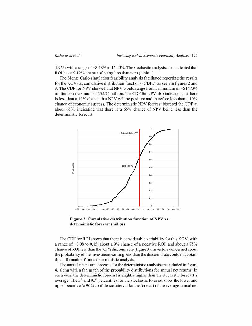
The Monte Carlo simulation feasibility analysis facilitated reporting the resultsfor the KOVs as cumulative distribution functions (CDFs), as seen in figures 2 and3. The CDF for NPV showed that NPV would range from a minimum of !$147.94million to a maximum of $35.74 million. The CDF for NPV also indicated that thereis less than a 10% chance that NPV will be positive and therefore less than a 10%chance of economic success. The deterministic NPV forecast bisected the CDF atabout 65%, indicating that there is a 65% chance of NPV being less than thedeterministic forecast.

The CDF for ROI shows that there is considerable variability for this KOV, witha range of !0.08 to 0.15, about a 9% chance of a negative ROI, and about a 75%chance of ROI less than the 7.5% discount rate (figure 3). Investors concerned aboutthe probability of the investment earning less than the discount rate could not obtainthis information from a deterministic analysis.

The annual net return forecasts for the deterministic analysis are included in figure4, along with a fan graph of the probability distributions for annual net returns. Ineach year, the deterministic forecast is slightly higher than the stochastic forecast’saverage. The 5th and 95th percentiles for the stochastic forecast show the lower andupper bounds of a 90% confidence interval for the forecast of the average annual net

Figure 2. Cumulative distribution function of NPV vs.deterministic forecast (mil $s)


Figure 3. Cumulative distribution function for return oninvestment vs. deterministic forecast (fraction)

Figure 4. Fan graph of net cash return vs. deterministicforecast (mil $s)


return. The fan graph for annual net return shows there is a 25% chance that netreturns will be less than !$5 million in year 3 and a 50% chance that net returns willbe negative after year 4.

Annual ending cash flows are of considerable interest to investors. A graph offorecasted annual ending cash reserves for the proposed plant is included in Figure5 for the deterministic and stochastic analyses. The deterministic analysis increas-ingly over-estimated average annual ending cash reserves each year of the planninghorizon. The fan graph forecasts a significant chance of negative cash reserves in allyears. The 90% confidence interval for annual ending cash reserves widens over theplanning horizon due to the compounding effect of risk on cash reserves.

Additional information available from a Monte Carlo simulation feasibilityanalysis could include probability distributions for financial ratios and other valuesof interest to the decision maker. For example, if the financing institution requiredthe debt-to-asset ratio to remain below 75%, the proposed ethanol plant would havea 13.6% chance of being declared insolvent over the 10-year planning horizon (table1). The probability that the investment will lose real net worth (i.e., a negativePVENW) is 6.46%, based on the probabilistic forecast for PVENW.

Conclusions

The purpose of this paper was to demonstrate the usefulness of Monte Carlosimulation for evaluating the economic viability of a proposed agribusiness. Asimulation model of a 50 MMGPY ethanol plant in the Texas Panhandle was

Figure 5. Fan graph of annual ending cash reserves vs. thedeterministic forecast (mil $s)


developed based on accepted input/output coefficients and investment costs.Stochastic values for costs and prices were incorporated into the model usinghistorical risk for these variables and recent forecasts of average annual prices, thusfacilitating a simulation risk analysis of the business.

The simulation model was developed using standard accounting principles andpro forma financial statements. Key output variables for the analysis were variablesof interest to potential investors: annual net return, present value of ending net worth(PVENW), net present value (NPV), rate of return to investment (ROI), probabilityof economic success, and annual cash flows. Additional output variables of interestto investors, such as financial ratios, could also be reported using a Monte Carlosimulation model.

The greatest benefit of a Monte Carlo simulation feasibility analysis is that themethodology explicitly incorporates risk faced by investors. By incorporatingprobability factors for variables that investors cannot forecast with certainty, theanalyst can develop realistic probabilistic forecasts of KOVs. Additional benefits ofthe methodology include the decision maker’s ability to see the range of KOVs aswell as the probabilities of unfavorable outcomes. Charts and probabilities, whichcan more accurately portray the probable outcomes for an investment than a singlepoint estimate, can be used to convey risky outcomes to the decision maker. Thesecharts and probabilities are particularly useful when the inherent risk in the proposedproject causes the KOV distributions to be skewed to the left or right or changeshape over time.

This paper demonstrated the advantages of simulation risk analysis to assess theinvestment potential of a proposed agribusiness. The methodology can be easilyapplied to feasibility studies for a wide variety of agribusinesses. With the widespread availability of micro computers, the use of spreadsheet models for business,and the ease of using simulation add-ins such as Simetar, models such as the onedemonstrated here can be easily developed and used for business decision makingin a risky environment.

References

Aven, T. (2005). Foundations of Risk Analysis. West Sussex, England: John Wiley &Sons, Ltd.

Bryan and Bryan International. (2001). “Dumas Texas area ethanol feasibility study.”Cotopaxi, CO: Bryan and Bryan International.

———. (2003). Ethanol Plant Development Handbook, 4th ed. Cotopaxi, CO: Bryan andBryan International.

———. (2006). “US and Canada fuel ethanol plant map.” Online. Available at http://www.bbiethanol.stores.yahoo.net/uscaetplmap.html. [Retrieved March 22, 2006].

Christianson, J. (2006). Christianson and Associates, PLLP. Personal communicationregarding costs of building an ethanol plant.

Economic Report of the President. (2006) US Government Printing Office, Washington,D.C.


FAPRI. (2006). “Baseline projections, November 2006.” Food and Agriculture PolicyResearch Institute, University of Missouri-Columbia.

Fruin, J., K. Rotsios, and D. W. Halbach. (1996). “Minnesota ethanol production and itstransportation requirements.” Staff Paper No. P96S7, Department of Applied Economics,University of Minnesota, Minneapolis, Minnesota.

Gill, R. C. (2002). “A stochastic feasibility study of Texas ethanol production: Analysisof Texas State Legislature ethanol subsidy.” Unpublished M.S. thesis, Department ofAgricultural Economics, Texas A&M University, College Station, Texas.

Hardaker, J. B., R. B. M. Huirne, J. R. Anderson, and G. Lien. (2004). Coping With Riskin Agriculture. Wallingford, Oxfordshire, UK: CABI Publishing.

Herbst, B. K. (2003). “The feasibility of ethanol production in Texas.” Unpublished M.S.thesis, Department of Agricultural Economics, Texas A&M University, CollegeStation, Texas.

Keller, G., and B. Warrack. (1997). Statistics for Management and Economics, 4th ed.Belmont, CA: Duxbury Press.

Long, E., and J. Creason. (1997). “Ethanol programs: A program evaluation report.”Report No. 97S04, Office of the Legislative Auditor, State of Minnesota.

Pouliquen, L. Y. (1970). “Risk analysis in project appraisal.” World Bank Staff OccasionalPapers (11), International Bank for Reconstruction and Development, The JohnHopkins University Press.

Ragsdale, C. T. (2001). Spreadsheet Modeling and Decision Analysis. New York: South-Western College Publishing.

Reutlinger, S. (1970). “Techniques for project appraisal under uncertainty.” World BankStaff Occasional Papers (10), International Bank for Reconstruction and Development,The John Hopkins University Press.

Richardson, J. W. (2006). “Simulation for applied risk management.” Unnumbered staffreport, Department of Agricultural Economics, Agricultural and Food Policy Center,Texas A&M University, College Station, Texas.

Richardson, J. W., S. L. Klose, and A. W. Gray. (2000). “An applied procedure forestimating and simulating multivariate empirical (MVE) probability distributions infarm-level risk assessment and policy analysis.” Journal of Agricultural and AppliedEconomics 32(2), 299S315.

Richardson, J. W., and H. P. Mapp, Jr. (1976). “Use of probabilistic cash flows inanalyzing investments under conditions of risk and uncertainty.” Southern Journal ofAgricultural Economics 8, 19S24.

Richardson, J. W., K. Schumann, and P. Feldman. (2006). “Simetar: Simulation for Excelto analyze risk.” Unnumbered staff report, Department of Agricultural Economics,Texas A&M University, College Station, Texas.

Shapouri, H., P. Gallagher, and M. Graboski. (2002). “USDA’s 1998 ethanol costs ofproduction survey.” Report No. 808, United States Department of Agriculture,Washington, DC.

Shapouri, H., M. Salassi, and J. N. Fairbanks. (2006). “The economic feasibility ofethanol production from sugar in the United States.” USDA-OEPNU and LouisianaState Univ. Online. Available at http://www.usda.gov/oce/EthanolSugarFeasibilityReport3.pdf. [Retrieved July 2006].


Smith, E. P., P. J. Harmelink, and J. R. Hasselback. (1998). CCH Federal Taxation:Comprehensive Topics. Chicago: CCH, Inc.

Thompson, J.R. (2000). Simulation: A Modeler’s Approach. New York: John Wiley &Sons, Inc.

Tiffany, D. G., and V. R. Eidman. (2003). “Factors associated with success of fuelethanol producers.” Staff Paper Series, Department of Applied Economics, Universityof Minnesota, Minneapolis, Minnesota.

United States Department of Agriculture. (2006). “Feed grains data delivery service.”Online. Available at http://www.ers.usda.gov/db/feedgrains. [Retrieved February 12,2007].

United States Department of Energy. (2006). “Alternative fuel vehicle fleet buyer’s guide:Incentives, regulations, contracts.” Online. Available at http://www.fleets.doe.gov.[Retrieved February 12, 2007].

Van Dyne, D. L. (2002). “Employment and economic benefits of ethanol production inMissouri.” Unnumbered staff report, Department of Agricultural Economics, Universityof Missouri-Columbia.

Vose, D. (2002). Risk Analysis: A Quantitative Guide. New York: John Wiley & Sons,Ltd.

Weida, N. C., R. Richardson, and A. Vazsonyi. (2001). Operations Analysis UsingMicrosoft ® Excel. Pacific Grove, CA: Duxbury.

Whims, J. (2004). “Corn-based ethanol costs and margins attachment 1.” Unnumberedstaff report, Agricultural Marketing Research Center, Department of AgriculturalEconomics, Kansas State University, Manhattan, Kansas.

Wilson, J. H., and B. Keating. (2002). Business Forecasting with Accompanying Excel-Based Forecast XTM Software. Boston: McGraw-Hill.

Winston, W. L. (1996). Simulation Modeling Using @Risk. New York: Duxbury Press.


Appendix: Stochastic Variables and Equations for the Ethanol Feasibility Model

Stochastic Variables

(A.1) Ethanol Pricet = Mean Pricet × [1 + MVE (Si F(Si), C8)] (A.2) DDGS Pricet = Mean Pricet × [1 + MVE (Si F(Si), C7)] (A.3) Corn Pricet = Mean Pricet × [1 + MVE (Si F(Si), C6)] (A.4) Gasoline Pricet = Mean Pricet × [1 + MVE (Si F(Si), C5)] (A.5) Natural Gas Pricet = Mean Pricet × [1 + MVE (Si F(Si), C4)] (A.6) Electricity Pricet = Mean Pricet × [1 + MVE (Si F(Si), C3)] (A.7) Inflation Ratet = Mean Ratet × [1 + MVE (Si F(Si), C2)] (A.8) Prime Interest Ratet = Mean Ratet × [1 + MVE (Si F(Si), C1)] (A.9) CD Interest Ratet = Prime Interest Ratet ! CD Wedge(A.10) OP Interest Ratet = Prime Interest Ratet ! OP Wedge(A.11) Down Timet = GRKS (minimum, middle, maximum)

Receipts

(A.12) Ethanol Productiont = Maximum Production per Dayt × (365 ! Down Timet )(A.13) Gasoline Requiredt = Ethanol Productiont × 0.05(A.14) Gross Ethanol Productiont = Ethanol Productiont + Gasoline Requiredt (A.15) Ethanol Receiptst = Gross Ethanol Productiont × Ethanol Pricet (A.16) Corn Usedt = Ethanol Productiont ' Conversion Rate(A.17) DDGS Receiptst = Corn Usedt × DDGS per bu Corn × DDGS Pricet(A.18) Interest Earnedt = Positive Cash Reservest!1 × CD Interest Ratet (A.19) Total Receiptst = Ethanol Receiptst + DDGS Receiptst + Interest Earnedt

Expenses

(A.20) Corn Costt = Corn Usedt × (Corn Pricet + Texas Price Wedget)(A.21) Gasoline Costt = Gasoline Requiredt × Gasoline Pricet(A.22) Natural Gas Costt = Ethanol Productiont × 0.038 × Natural Gas Pricet(A.23) Electricity Costt = Ethanol Productiont × 0.8 × Electricity Pricet(A.24) Other Costst = VC ' gallont!1 × (1 + Inflation Ratet) × Ethanol Productiont(A.25) Total Variable Costt = Corn Costt + Gasoline Costt + Natural Gas Costt +

Electricity Costt + Other Costst(A.26) Plant Debt Interestt = Principal Owedt × Fixed Interest Ratet(A.27) Operating Interestt = Total Variable Costt × OP Interest Ratet × Fraction

of year(A.28) Carryover Loan Interestt = Cashflow Deficitst!1 × OP Interest Ratet(A.29) Total Interest Costt = Plant Debt Interestt + Operating Interestt + Carryover

Loan Interestt(A.30) Depreciationt = Plant Cost × MACRSt + Capital Replacementt × MACRSt(A.31) Total Expensest = Total Variable Costt + Total Interest Costt + Depreciationt


(A.32) Net Returnst = Total Receiptst ! Total Expensest(A.33) Net Cash Incomet = Total Receiptst ! Total Variable Costst ! Total Interest

Costt

Cashflow

(A.34) Cash Inflowst = Net Cash Incomet + Positive Cash Reservest!1(A.35) Dividendst = Maximum [ 0.0, Net Returnst × 0.35](A.36) Principal Paymentt = Fixed Annual Payment ! Plant Debt Interestt(A.37) Federal Income Taxest = Positive Net Returnst × Income Tax Rate(A.38) Cash Outflowst = Principal Paymentt + Repay Cashflow Deficitt!1 + Capital

Replacementt + Dividendst + Federal Income Taxest(A.39) Ending Casht = Cash Inflowst ! Cash Outflowst

Balance Sheet

(A.40) Assetst = Land Value + Book Value Plantt + Positive Ending Casht(A.41) Liabilitiest = Plant Debtt!1 ! Principal Paymentst + Negative Ending Casht(A.42) Net Wortht = Assetst ! Liabilitiest

Financial Ratios and KOVs (A.43) NPV = ! Beginning Net Worth + 3 (Dividendsi + ΔNet Worthi) ' (1 + 0.075)i

(A.44) PVENW = Net Worth10 ' (1 + 0.075)10

(A.45) D/At = Liabilitiest ' Net Wortht(A.46) ROIt = (Net Returnst + Total Interest Costt ) ' Initial Plant Cost

Online Applicant Tracking System User's Guide

Documents

Transcript of Online Applicant Tracking System User's Guide