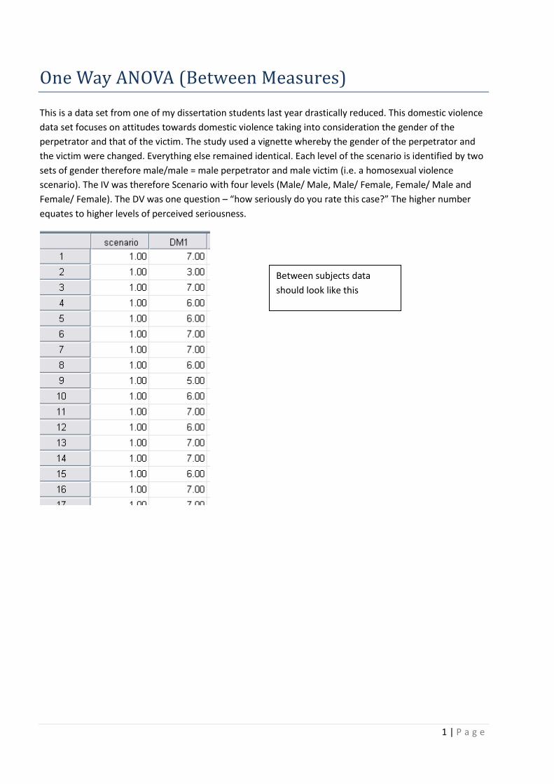
1 | P a g e

One Way ANOVA (Between Measures)

This is a data set from one of my dissertation students last year drastically reduced. This domestic violence

data set focuses on attitudes towards domestic violence taking into consideration the gender of the

perpetrator and that of the victim. The study used a vignette whereby the gender of the perpetrator and

the victim were changed. Everything else remained identical. Each level of the scenario is identified by two

sets of gender therefore male/male = male perpetrator and male victim (i.e. a homosexual violence

scenario). The IV was therefore Scenario with four levels (Male/ Male, Male/ Female, Female/ Male and

Female/ Female). The DV was one question – “how seriously do you rate this case?” The higher number

equates to higher levels of perceived seriousness.

Between subjects data

should look like this

2 | P a g e

Analyze > General Linear Model > Univariate

Your Variables will

appear here – be

sure you know

which one is the IV

and which is the DV

Place your DV in the

‘Dependent Variable’

box

And the IV in the

‘Fixed Factor(s)’ box

Select Options

3 | P a g e

Your IV appears

here > select it and

put it across to

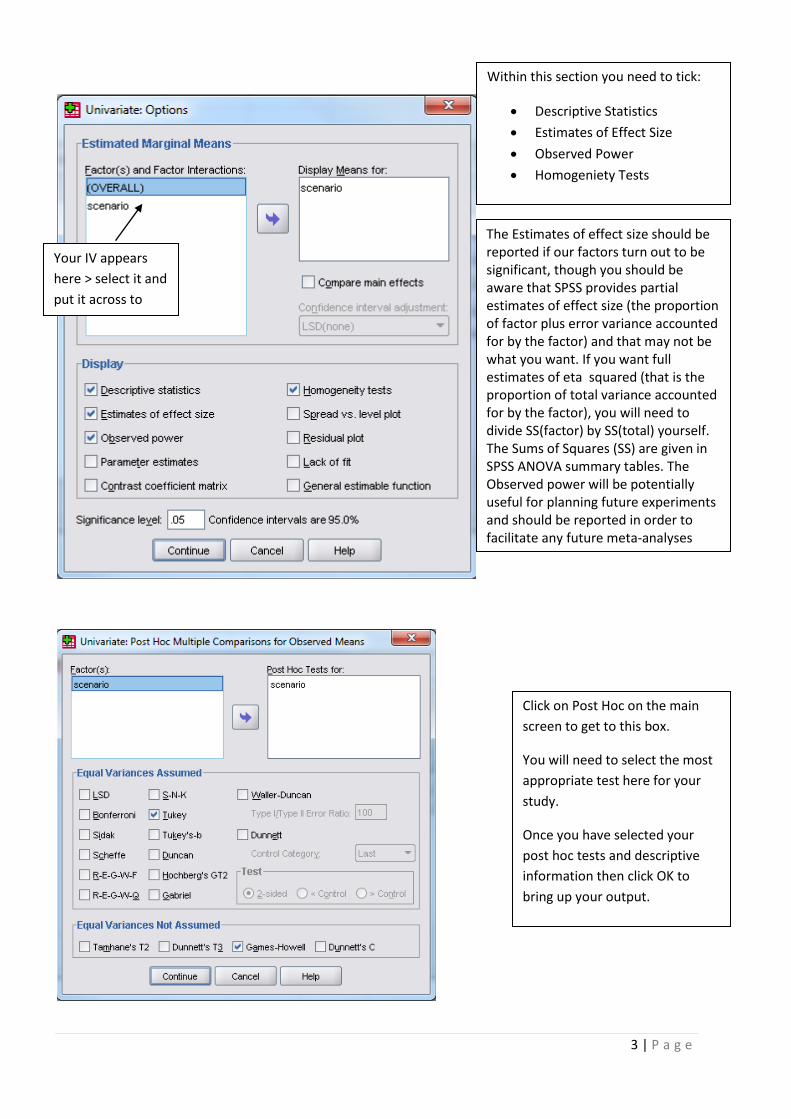
Within this section you need to tick:

Descriptive Statistics

Estimates of Effect Size

Observed Power

Homogeniety Tests

Click on Post Hoc on the main

screen to get to this box.

You will need to select the most

appropriate test here for your

study.

Once you have selected your

post hoc tests and descriptive

information then click OK to

bring up your output.

The Estimates of effect size should be reported if our factors turn out to be significant, though you should be aware that SPSS provides partial estimates of effect size (the proportion of factor plus error variance accounted for by the factor) and that may not be what you want. If you want full estimates of eta squared (that is the proportion of total variance accounted for by the factor), you will need to divide SS(factor) by SS(total) yourself. The Sums of Squares (SS) are given in SPSS ANOVA summary tables. The Observed power will be potentially useful for planning future experiments and should be reported in order to facilitate any future meta-analyses

4 | P a g e

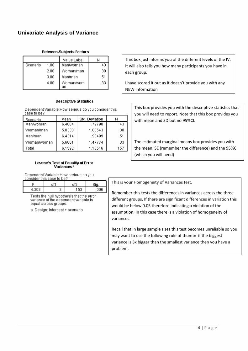
Univariate Analysis of Variance

This box just informs you of the different levels of the IV.

It will also tells you how many participants you have in

each group.

I have scored it out as it doesn’t provide you with any

NEW information

This box provides you with the descriptive statistics that

you will need to report. Note that this box provides you

with mean and SD but no 95%CI.

The estimated marginal means box provides you with

the mean, SE (remember the difference) and the 95%CI

(which you will need)

This is your Homogeneity of Variances test.

Remember this tests the differences in variances across the three

different groups. If there are significant differences in variation this

would be below 0.05 therefore indicating a violation of the

assumption. In this case there is a violation of homogeneity of

variances.

Recall that in large sample sizes this test becomes unreliable so you

may want to use the following rule of thumb: if the biggest

variance is 3x bigger than the smallest variance then you have a

problem.

5 | P a g e

The above box is the main table needed for your write up...

You should be reading the line that contains the name of the IV only with addition of the error df

for write up.

One way Between Measures ANOVA indicated a significant difference between two or more groups: F(3, 153) = 6.178, p < 0.001, pη2 = 0.108, observed power = 0.960 Remember Partial eta squared or pη2

is the effect size calculation for ANOVA

Observed Power may be useful for future research so report it.

The 95% CI within this table should be reported with your descriptive statistics. Very briefly they indicate where the true population mean is.

6 | P a g e

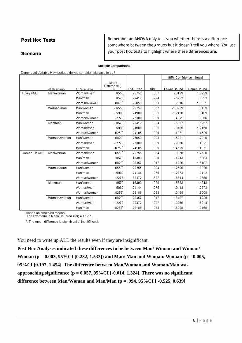
You need to write up ALL the results even if they are insignificant.

Post Hoc Analyses indicated these differences to be between Man/ Woman and Woman/

Woman (p = 0.003, 95%CI [0.232, 1.533]) and Man/ Man and Woman/ Woman (p = 0.005,

95%CI [0.197, 1.454]. The difference between Man/Woman and Woman/Man was

approaching significance (p = 0.057, 95%CI [-0.014, 1.324]. There was no significant

difference between Man/Woman and Man/Man (p = .994, 95%CI [ -0.525, 0.639]

Remember an ANOVA only tells you whether there is a difference

somewhere between the groups but it doesn’t tell you where. You use

your post hoc tests to highlight where these differences are.

7 | P a g e

One Way Repeated Measures ANOVA

Analyze > General Linear Model > Repeated Measures

Within subjects data

set should look like this.

This box simply indicates if some of

your levels of the IV can be grouped

together as one. In this case, due to all

being significantly different from one

another, there are no homogenous

subsets.

8 | P a g e

Once you have done this you will need to click on Options.

This is the first box that will appear.

This is where you tell the computer

how many levels of your IV you have.

In this case we have 3

Therefore we name the Within

Subjects Factor

And state the Number of Levels

Click Add.

Click Define once it is highlighted

Your Levels of your

IV will appear here.

You need to select

them and place

them into the

Within Subjects

Variables box

9 | P a g e

This is what your output should look like... be warned that there is a lot of ‘useless’ information in

this output.

General Linear Model

Within-Subjects Factors

Measure:MEASURE_1

Stroop

Dependent

Variable

1 baseline

2 rhyming

3 incongr

This is the Options Box

You will need to select your IV and

place it into Display Means for

Tick on the usual

Descriptive statistics

Estimates of effect size

Observed power

You do not need to tick the

‘Homogeneity Tests’ box as this only

relates to between subjects IV.

For post hoc tests in repeated

measures you select ‘Compare Main

Effects’ and select the appropriate

measure from the dropdown menu.

See information for between subject

ANOVA to learn about Partial eta and

observed power

Click Continue once finished

This box only informs you of the levels

of your IV.

You do not need to report this box

10 | P a g e

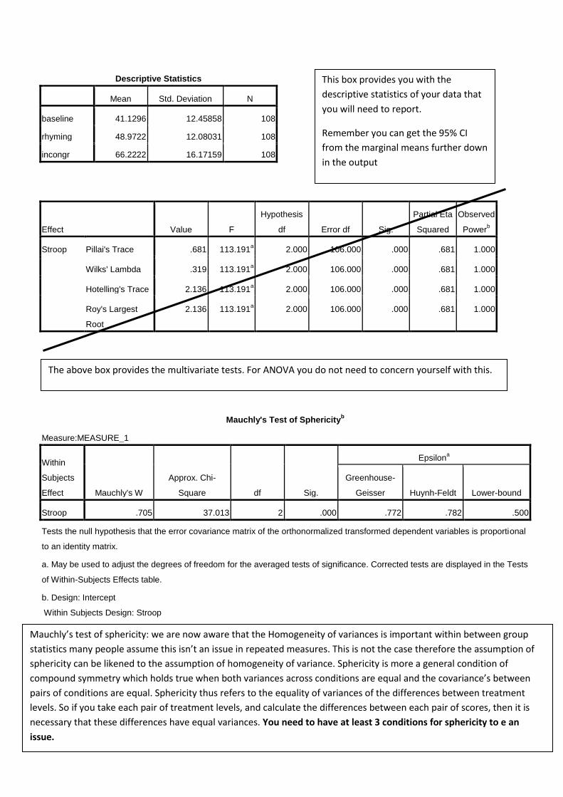
Descriptive Statistics

Mean Std. Deviation N

baseline 41.1296 12.45858 108

rhyming 48.9722 12.08031 108

incongr 66.2222 16.17159 108

Effect Value F

Hypothesis

df Error df Sig.

Partial Eta

Squared

Observed

Powerb

Stroop Pillai's Trace .681 113.191a 2.000 106.000 .000 .681 1.000

Wilks' Lambda .319 113.191a 2.000 106.000 .000 .681 1.000

Hotelling's Trace 2.136 113.191a 2.000 106.000 .000 .681 1.000

Roy's Largest

Root

2.136 113.191a 2.000 106.000 .000 .681 1.000

Mauchly's Test of Sphericityb

Measure:MEASURE_1

Within

Subjects

Effect Mauchly's W

Approx. Chi-

Square df Sig.

Epsilona

Greenhouse-

Geisser Huynh-Feldt Lower-bound

Stroop .705 37.013 2 .000 .772 .782 .500

Tests the null hypothesis that the error covariance matrix of the orthonormalized transformed dependent variables is proportional

to an identity matrix.

a. May be used to adjust the degrees of freedom for the averaged tests of significance. Corrected tests are displayed in the Tests

of Within-Subjects Effects table.

b. Design: Intercept

Within Subjects Design: Stroop

Mauchly’s test of sphericity: we are now aware that the Homogeneity of variances is important within between group

statistics many people assume this isn’t an issue in repeated measures. This is not the case therefore the assumption of

sphericity can be likened to the assumption of homogeneity of variance. Sphericity is more a general condition of

compound symmetry which holds true when both variances across conditions are equal and the covariance’s between

pairs of conditions are equal. Sphericity thus refers to the equality of variances of the differences between treatment

levels. So if you take each pair of treatment levels, and calculate the differences between each pair of scores, then it is

necessary that these differences have equal variances. You need to have at least 3 conditions for sphericity to e an

issue.

This box provides you with the

descriptive statistics of your data that

you will need to report.

Remember you can get the 95% CI

from the marginal means further down

in the output

The above box provides the multivariate tests. For ANOVA you do not need to concern yourself with this.

11 | P a g e

Source

Type III Sum

of Squares df Mean Square F Sig.

Partial Eta

Squared

Observed

Powera

Stroop Sphericity Assumed 35593.521 2 17796.760 170.888 .000 .615 1.000

Greenhouse-Geisser 35593.521 1.545 23042.091 170.888 .000 .615 1.000

Huynh-Feldt 35593.521 1.563 22772.168 170.888 .000 .615 1.000

Lower-bound 35593.521 1.000 35593.521 170.888 .000 .615 1.000

Error(Stroop) Sphericity Assumed 22286.530 214 104.143

Greenhouse-Geisser 22286.530 165.285 134.837

Huynh-Feldt 22286.530 167.244 133.258

Lower-bound 22286.530 107.000 208.285

The highlighted aspects are those that need writing up.

Why use the Greenhouse-Geisser? The Greenhouse-Geisser is used when Sphericity cannot be

assumed. However, authors often recommend that this is used all the time. When reporting the

Greenhouse-Geiser df round the figures up.

Source Stroop

Type III Sum of

Squares df Mean Square F Sig.

Partial Eta

Squared

Observed

Powera

Stroop Linear 34000.543 1 34000.543 228.356 .000 .681 1.000

Quadratic 1592.978 1 1592.978 26.821 .000 .200 .999

Error(Stroop) Linear 15931.540 107 148.893

Quadratic 6354.990 107 59.392

Source

Type III Sum of

Squares df Mean Square F Sig. Partial Eta Squared Observed Powera

Intercept 879739.447 1 879739.447 2482.440 .000 .959 1.000

Error 37919.194 107 354.385

The above two boxes can be ignored – you do not need to write them up or understand what they tell you

12 | P a g e

Estimated Marginal Means – these provide you with the 95% CI of the mean that you will need for writing up. Stroop

Estimates

Measure:MEASURE_1

Stroop Mean Std. Error

95% Confidence Interval

Lower Bound Upper Bound

1 41.130 1.199 38.753 43.506

2 48.972 1.162 46.668 51.277

3 66.222 1.556 63.137 69.307

Pairwise Comparisons

Measure:MEASURE_1

(I) Stroop

(J)

Stroop

Mean Difference (I-

J) Std. Error Sig.a

95% Confidence Interval for Differencea

Lower Bound Upper Bound

1 2 -7.843* .980 .000 -9.785 -5.900

3 -25.093* 1.661 .000 -28.384 -21.801

2 1 7.843* .980 .000 5.900 9.785

3 -17.250* 1.438 .000 -20.101 -14.399

3 1 25.093* 1.661 .000 21.801 28.384

2 17.250* 1.438 .000 14.399 20.101

Based on estimated marginal means

*. The mean difference is significant at the .05 level.

a. Adjustment for multiple comparisons: Least Significant Difference (equivalent to no adjustments).

When writing up the post hoc tests ensure you write up ALL tests including those that are not

significant. You will also need to report the 95% CI. Notice that these are now the 95% CI of the

DIFFERENCE. If these intervals include or go through 0 then this will be reflected in the

significance value.

13 | P a g e

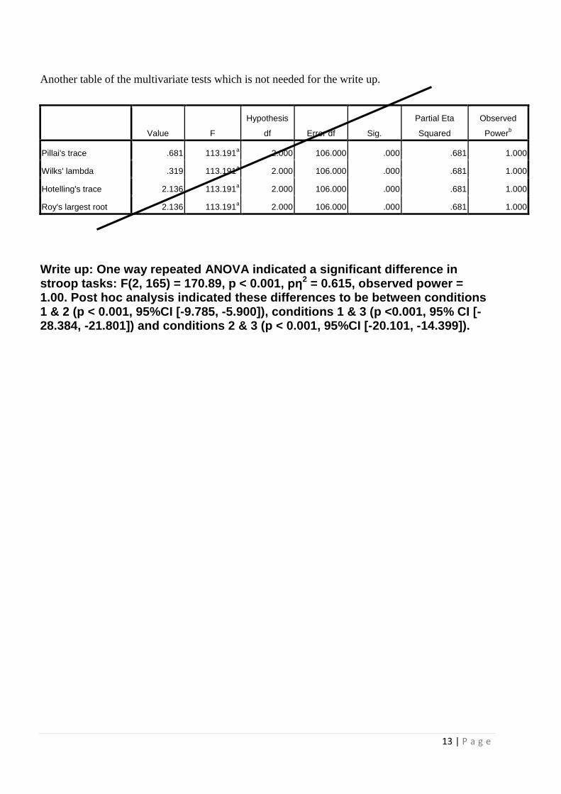
Another table of the multivariate tests which is not needed for the write up.

Value F

Hypothesis

df Error df Sig.

Partial Eta

Squared

Observed

Powerb

Pillai's trace .681 113.191a 2.000 106.000 .000 .681 1.000

Wilks' lambda .319 113.191a 2.000 106.000 .000 .681 1.000

Hotelling's trace 2.136 113.191a 2.000 106.000 .000 .681 1.000

Roy's largest root 2.136 113.191a 2.000 106.000 .000 .681 1.000

Write up: One way repeated ANOVA indicated a significant difference in stroop tasks: F(2, 165) = 170.89, p < 0.001, pη2 = 0.615, observed power = 1.00. Post hoc analysis indicated these differences to be between conditions 1 & 2 (p < 0.001, 95%CI [-9.785, -5.900]), conditions 1 & 3 (p <0.001, 95% CI [-28.384, -21.801]) and conditions 2 & 3 (p < 0.001, 95%CI [-20.101, -14.399]).

14 | P a g e

Non- Parametric Equivalents: Between Measures – Kruskal Wallis

Analyze > K Independent Samples

Place your DV into the ‘Test Variable

List’

Place your IV into the ‘Grouping

Variable’ and then select ‘Define

Groups’

This will bring up a separate dialogue

box. Here you need to state the

minimum and maximum range for the

IV

Once this has been done click continue

and then OK

15 | P a g e

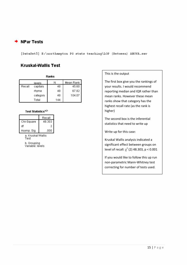
This is the output

The first box give you the rankings of

your results. I would recommend

reporting median and IQR rather than

mean ranks. However these mean

ranks show that category has the

highest recall rate (as the rank is

higher)

The second box is the inferential

statistics that need to write up

Write up for this case:

Kruskal Wallis analysis indicated a

significant effect between groups on

level of recall: χ2 (2) 48.303, p < 0.001

If you would like to follow this up run

non-parametric Mann-Whitney test

correcting for number of tests used.

16 | P a g e

Non- Parametric Equivalents: Within Measures – Freedman

Analyze> Non Parametric tests> K Related Tests

Select all the levels of the

variables of interest and

place them over into ‘test

variables’

Then select OK

Mean ranks as before. This indicates

that the incongruent group has the

longest time to read through the list.

Test statistics are needed for your

write up

Thus for this study

Freedman test indicates a significant

difference between the groups on

speed of reading: χ2 (2) 145.814, p <

0.001

If you would like to follow this up run

non-parametric wilcoxen test

correcting for number of tests used.