Once Poor, Always Poor? Do Initial Conditions Matter? Evidence from …ftp.iza.org/dp5971.pdf ·...
27
DISCUSSION PAPER SERIES Forschungsinstitut zur Zukunft der Arbeit Institute for the Study of Labor Once Poor, Always Poor? Do Initial Conditions Matter? Evidence from the ECHP IZA DP No. 5971 September 2011 Eirini Andriopoulou Panos Tsakloglou
Transcript of Once Poor, Always Poor? Do Initial Conditions Matter? Evidence from …ftp.iza.org/dp5971.pdf ·...

DI
SC
US
SI
ON
P
AP
ER
S
ER
IE
S
Forschungsinstitut zur Zukunft der ArbeitInstitute for the Study of Labor
Once Poor, Always Poor? Do Initial Conditions Matter? Evidence from the ECHP
IZA DP No. 5971
September 2011
Eirini AndriopoulouPanos Tsakloglou

Once Poor, Always Poor?
Do Initial Conditions Matter? Evidence from the ECHP
Eirini Andriopoulou Athens University of Economics and Business
Panos Tsakloglou
Athens University of Economics and Business and IZA
Discussion Paper No. 5971 September 2011
IZA
P.O. Box 7240 53072 Bonn
Germany
Phone: +49-228-3894-0 Fax: +49-228-3894-180
E-mail: [email protected]
Any opinions expressed here are those of the author(s) and not those of IZA. Research published in this series may include views on policy, but the institute itself takes no institutional policy positions. The Institute for the Study of Labor (IZA) in Bonn is a local and virtual international research center and a place of communication between science, politics and business. IZA is an independent nonprofit organization supported by Deutsche Post Foundation. The center is associated with the University of Bonn and offers a stimulating research environment through its international network, workshops and conferences, data service, project support, research visits and doctoral program. IZA engages in (i) original and internationally competitive research in all fields of labor economics, (ii) development of policy concepts, and (iii) dissemination of research results and concepts to the interested public. IZA Discussion Papers often represent preliminary work and are circulated to encourage discussion. Citation of such a paper should account for its provisional character. A revised version may be available directly from the author.

IZA Discussion Paper No. 5971 September 2011
ABSTRACT
Once Poor, Always Poor? Do Initial Conditions Matter? Evidence from the ECHP
The paper analyzes the effects of individual and household characteristics on current poverty status, while controlling for initial conditions, past poverty status and unobserved heterogeneity in 14 European Countries for the period 1994-2000, using the European Community Household Panel. The distinction between true state dependence and individual heterogeneity has very important policy implications, since if the former is the main cause of poverty it is of paramount importance to break the “vicious circle” of poverty using income-supporting social policies, whereas if it is the latter anti-poverty policies should focus primarily on education, training, development of personal skills and other labour market oriented policies. The empirical results are similar in qualitative but rather different in quantitative terms across EU countries. State dependence remains significant in all specifications, even after controlling for unobserved heterogeneity or when removing possible endogeneity bias. JEL Classification: I32, I38 Keywords: poverty dynamics, EU, ECHP Corresponding author: Panos Tsakloglou Athens University of Economics and Business 76 Patission Street Athens 10434 Greece E-mail: [email protected]

2
1. INTRODUCTION In recent years, issues of state dependence feature prominently in poverty
dynamics research. The main hypothesis tested in this research is whether past poverty
experiences determine current poverty status. This may happen, for instance, because
poverty spells might result in depreciation of human capital and employment skills,
causing low-pay or unemployment spells and, finally, increasing the duration or the
frequency of poverty spells (poverty reoccurrence). If the long run policy objective is to
keep poverty rates low and state dependence is ‘genuine’, then it is important to bring
individuals out of poverty using social benefits in the short run. Nevertheless, the state
dependence usually observed in dynamic panel data models may also be attributed to
sorting effects, in the sense that the individuals that escape poverty may possess
particular observed (e.g. age, educational qualifications, etc) or unobserved
characteristics (willingness to escape poverty, cleverness, social networks, life attitudes,
etc) and, thus, differ in a systematic way from the individuals that remain poor.
Consequently, when examining state dependence it is important to control for observed
as well as unobserved heterogeneity. Further, a positive result in terms of state
dependence may also be due to the fact that individuals with a higher tendency to remain
permanently poor may be over-represented in the sample. Therefore, in the case of state
dependence, controlling for the observed and unobserved determinants of initial poverty
status (initial conditions) is also important.
In the current paper, we follow the methodology of Wooldridge (2005), which
proposes a solution that handles simultaneously the problems of endogeneity of the
initial conditions and unobserved heterogeneity. He suggests using a joint density
distribution conditional on the strictly exogenous variables and the initial condition,
instead of attempting to obtain the joint distribution of all outcomes of the endogenous
variables. In this analysis, a multivariate random effects logit estimation has been
employed for the analysis of poverty state dependence in 14 EU Member-States during
the period 1994-2000 using the data of the European Community Household Panel
(ECHP).
In the next two sections, the issues of unobserved heterogeneity and initial
conditions are discussed drawing evidence from previous studies in poverty,
employment and low-pay dynamics. The ECHP is briefly presented in section 4 along
with household income and poverty definitions. Section 5, presents the model to be
applied. The last two sections report the empirical results and the conclusions of our
analysis, along with some policy implications.
2. TRUE STATE DEPENDENCE VERSUS UNOBSERVED
HETEROGENEITY True state dependence means that the experience of poverty in one year per se
raises the risk of being poor in the next year (Heckman 1981a). However, since
individuals with “favourable” characteristics are likely to leave poverty earlier, the state
or duration dependence observed in data may not be genuine. Therefore it is important

3
along with the effect of time to control also for observed as well as unobserved
heterogeneity.1
In recent years, researchers focus on the distinction between true state dependence
and individual heterogeneity. This distinction has very important policy implications. For
instance, if true state dependence is indeed significant compared to individual
heterogeneity, then it is important to break the “vicious circle” of poverty and try, even at
high cost, to bring individuals out of poverty using income-support policies such as
social benefits. On the contrary, if individual heterogeneity defines the duration of
poverty, anti-poverty policies should focus on other schemes such as education,
development of personal skills and capacities or other labour market and social policies.
Most studies find that poverty state dependence remains significant even when
controlling for unobserved heterogeneity. Canto (1996) examines the duration
dependence for poverty entries and exits in Spain using a non-parametric specification
for the hazard rate. She controls for unobserved heterogeneity indirectly by testing the
homogeneity of the hazard rate between groups that are likely to have different spell
lengths. She finds significant duration dependence both for poverty re-entries and exits.
Cappellari and Jenkins (2004) using data from the BHPS for the 1990s conclude that
there is substantial state dependence in poverty, separately from the persistence caused
by heterogeneity. Poggi (2007) studies social exclusion dynamics in Spain and also finds
that both individual heterogeneity and true state dependence are related to the probability
of experiencing social exclusion. Biewen (2006) reports that even after controlling for
observed and unobserved individual characteristics, there is negative state dependence in
poverty exit and re-entry behaviour. He also calculates that 6% of the German population
has unobserved characteristics that lead to low poverty exit and high re-entry rates, thus
making these individuals possible candidates for chronic poverty. According to Ayllón
(2008), in Spain more than 50% of aggregate state dependence in poverty status is due to
past poverty experiences. Finally, when focusing on youth poverty, while separating
genuine state dependence in the poverty status from observed and unobserved
characteristics, Ayllon (2009) concludes that there is a substantial proportion of genuine
state dependence in the poverty status.
On the other hand, Giraldo et al. (2002) stress that there are two sources of
unobserved heterogeneity related to the study of poverty: first, the ability of household
members to obtain income in a specific period and, second, the way in which this ability
evolves over time. When allowing for time-variant unobserved heterogeneity, the authors
1 State and duration dependence are often used in the literature are synonyms. However, state dependence
determines how the probability to be poor in the current period depends on whether the individual was poor
in the previous period, while duration dependence indicates how the probability to be poor in the current
period depends on the duration spent in the poverty spell. This means that when duration dependence is
examined, more than one lagged values of the dependent variable are used in the regression, or when
poverty exits or re-entries are examined (instead of poverty status per se), more than one period dummies
are included in the hazard function. This paper focuses on state dependence rather than duration
dependence. Further, since the paper focuses on the effect on time on poverty status per se, the literature of
poverty entries and exits is not presented explicitly (see, for example, Jenkins (1995; 2000), Stevens
(1999), Antolin et al. (1999), Muffels (2000), Oxley et al. (2000), OECD (2001), Jenkins et al. (2001),
Canto (2002, 2003), Devicienti (2002; 2010), Finnie and Sweetman (2003), Fouarge and Layte (2005) and
Callens and Croux (2009)). A literature review covering these papers as well as an analysis of poverty
transitions in Europe using discrete-time proprotional hazard rate models with the ECHP data is presented
in Andriopoulou (2009: ch. VI, VII) and Andriopoulou and Tsakloglou (2011).

4
do not find any sign of true state dependence in their analysis of persistent poverty in
Italy. This finding reinforces the theory of incentives of the poor which may vary not
only among individuals but also with time. As underlined by Aassve et al. (2006), there
is also another issue on whether it is poverty experience or low income experience that
really affects individuals with regards to the duration dependence. Poverty spells are not
like unemployment spells, during which the individual is completely aware of the
situation and, hence, his choices and preferences might be affected by his position.
Studies that focus on low pay instead of poverty (Stewart and Swaffield 1999; Cappellari
2004; Stewart 2007)2 show that the probability of being low paid depends strongly on
low pay in the previous year. In the same line, Finnie and Gray (2002), when examining
individual mobility across earning quintiles, conclude that the probability of having an
upward or downward transition depends negatively on the time that an individual has
spent in a given quintile and this negative duration dependence remains significant when
controlling for unobserved heterogeneity. Likewise, Weber (2002) verifies that there is
significant state dependence for women at the lower part of the distribution in Austria.
It should be noted that Cockx and Dejemeppe (2005) assert that the observed
negative duration dependence in the exit rate very often turns out to be spurious, at least
in unemployment studies. Nevertheless, Caliendo and Uhlendorff (2008) analyze the
mobility between self-employment, wage employment and non-employment and find
strong true state dependence in all three states. With regards to the labour force
participation, Hyslop (1999) shows that participation decisions for women are
characterized by significant state dependence, unobserved heterogeneity and feedback
effects from fertility to participation decisions and vice versa.
3. THE INITIAL CONDITIONS PROBLEM The initial conditions problem, developed by Heckman (1981b), in terms of
transitions analysis, can be summarised to the fact that those who are poor in the first
year of the survey may be a non-random sample of the population. Specifically, a
positive result in terms of state dependence may be due to the fact that individuals with a
higher tendency to remain permanently poor may be over-represented in the sample
(Cappellari and Jenkins 2004; 2008). Therefore, in the case of state dependence,
controlling for the observed and unobserved determinants of initial poverty status is
important.
In practice, the problem arises because the start of the observation period does not
concise with the start of the stochastic process that has generated the poverty or non-
poverty experiences. Arulampalam et al. (2000) emphasize that even if the model
controls for unobserved heterogeneity, in order to disentangle the effect of state
dependence from unobserved heterogeneity, the initial conditions need to be modelled
instead of assumed as exogenously given, because the initial conditions may be
correlated with the unobservables.
The problem of initial conditions has been tackled more extensively in the
literature of unemployment dynamics. Arulampalam et al. (2000) examine
unemployment dynamics for men using the BHPS and introduce the econometric issues
2 Stewart (2007) focuses more on how past low-pay employment affects the probability of being
unemployed in the future using a similar methodology as when state dependence is examined.

5
concerning dynamic panel data models: unobserved heterogeneity (based on
Chamberlain 1984), state dependence (based on Heckman 1981a, 1981c) and the initial
conditions problem (based on Heckman 1981b). Even when controlling for initial
conditions and unobserved heterogeneity, they find that there is strong state dependence
especially for older unemployed individuals that may be attributed to depreciation of
human capital, signalling (in the sense that past unemployment spells signal the
capacities or productivity of individuals to potential employers) and to the fact that
unemployed individuals may accept low quality jobs and this may lead to enterprise
closure and future unemployment spells. Arulampalam (2002) extents this work further
in various directions, using different definitions of unemployment.
Cappellari and Jenkins (2004) use a first-order Markov model in order to study
poverty transitions3. The great virtue of this model, which is a complement to hazard and
covariance structure models, is that it allows controlling for initial conditions effects. In
addition, these models control for potential non-random sample retention (for individuals
that do no attrite and for whom income is observed for at least two consecutive periods).
Ayllón (2008) examines poverty transitions in Spain using the model proposed by
Cappellari and Jenkins (2004). She finds that unobserved heterogeneity affecting poverty
status in the base year as well as sample attrition, are exogenous to unobservables related
to poverty transitions (although her results are sensitive to the selection of the poverty
line). Models that control for initial conditions are also used in studies of earnings
mobility (Stewart and Swaffield 1999; Cappellari 2004; Cappellari and Jenkins 2008).
The methodology that we use in this paper in order to control for initial conditions
is based on Wooldridge (2005), which proposes a solution to handle the problem of
endogeneity of the initial conditions, while controlling for unobserved. He suggests using
a joint density distribution conditional on the strictly exogenous variables and the initial
condition, instead of attempting to obtain the joint distribution of all outcomes of the
endogenous variables (Hsiao 1986). For the binary response models of probit and logit
form, the main advantage of this method is that it can be applied easily using standard
random effects software. Yet, the explanatory variables included in the model must be
strictly exogenous and at most one lag4 of the dependent variable can be used in the
estimation. Another restriction of the model is that it can be applied only to balanced
panel data. This reduction from unbalanced to balanced panel data can always result in
discarding useful information. An application of this methodology to social exclusion can
be found in Poggi (2007).
4. THE EUROPEAN COMMUNITY HOUSEHOLD PANEL AND
DEFINITIONS The empirical research of the paper is based on the data of the European
Community Household Panel (ECHP). The ECHP is a harmonized cross-national
longitudinal survey, focusing on income and living conditions of households and
individuals in the European Union. Due to its multidimensional nature, the ECHP
provides information at micro-level across countries and across time on: income,
3 Schluter (1997) also uses a Markov model with exogenous variables in order to study the German income
mobility, with some extensions to poverty dynamics. 4 D' Addio and Honore (2002) claim that the probability of exiting poverty may depend not only on the
poverty status of the last period, but on the poverty status in the two most recent periods and they model
second order state dependence, while controlling time–varying explanatory variables.

6
employment, health, education, housing, migration, social transfers and social
participation, as well as demographics. In other words, as Eurostat describes it, ECHP
offers data on EU social dynamics (Eurostat 2003). The duration of the survey is eight
years; thus, the ECHP consists of eight waves, one for each year, from 1994 to 2001.
The ECHP covers all the 15 Member-States of the EU in that period, but not all countries
have participated in all waves. In addition some Member-States, such as the UK and
Germany, used data from existing panel surveys and converted them to ECHP format. In
the current paper, we use all eight waves of the ECHP for 14 EU Member-States5.
Most of the income components in the ECHP have an annual time frame of the
calendar year preceding the interview. In all the ECHP countries, apart from the UK, the
calendar year coincides with the tax year, which is the reference period for income
components. Although, in this way income comparability is ensured, other variables like
the household composition variables, the economic activity status etc. refer to the time of
interview and might not relate well to income measured over a period up to twelve
months in the past (Eurostat 2001). This is particularly undesirable for poverty dynamic
analysis that tries to identify changes in income components and also uses the lagged
poverty status as an explanatory variable. Therefore, for the needs of the dynamic
analysis that follows, we have reconstructed the household income, transferring all the
income components one year back.6
Following the practice of Eurostat, the poverty line used in the paper is set at 60%
of the national median equivalised household income per capita, as it has been calculated
using the modified OECD scale which assigns 1 to the first adult, 0.5 to the remaing
adults and 0.3 to children.
5. THE MODEL AND ECONOMETRIC DETAILS OF THE ANALYSIS The main difference of the model used in this paper from a typical hazard model
examining state dependence is that the dependent variable is the poverty status per se
(whether someone is poor or non-poor) and not a variable signalling the poverty entry or
exit. Moreover, state dependence is not captured with time dummies, but with the lagged
value of the dependent variable. According to Wooldridge (2005, p. 42), only one lag of
the dependent variable can be used when controlling for initial conditions. Nevertheless,
this means that we cannot measure duration dependence, how much the chances of
exiting poverty fall the longer one is in poverty.7 Initial conditions are captured by
introducing in the regression the value of the dependent variable in the first period. In
this way, the assumption of exogeneity of all the explanatory variables is a strong
assumption and, therefore, is tested at the end of the analysis.
5 For Sweden only cross-sectional data are available and, therefore, Sweden has been excluded from the
analysis. Moreover, the panels of Austria, Finland and Luxembourg are shorter than those of the other
countries. 6 It should be underlined that we do not simply lag one wave back the total net household income, but we
take into account the different composition that each household might had in the previous have. The
methodology developed for the reconstruction of household income follows the logic of Eurostat’s (2003a)
construction of household income variable and is similar to the one applied by Debels and Vandecasteele
(2008).The algorithm for the reconstruction of household income is available from the authors on request. 7 This effect can only be captured when modelling poverty exit with hazard functions using time dummies
so as to capture the increasing effect of state dependence year by year.

7
More specifically for a random individual in the population and t=1, 2, … T, the
conditional probability that poverty occurs is:
, 1 0 , 1( 1| ,..., , , ) ( )it i t i i i it i t iP y y y z c z y cγ ρ− −= = Φ + + (1)
Where ity is the dependent variable or the poverty state of the individual i at
period t (when 1ity = the individual is poor in period t and when 0ity = the individual
is non-poor), ( )xΦ is the logistic function exp( )( ) ( )
1 exp( )
xx x
xΦ = = Λ
+, which is between zero
and one for all real numbers x , γ and ρ are the parameters to be estimated, iz and itz
are the vectors of time constant and time-varying explanatory variables and ic is the
unobserved effect. ρ is the coefficient of the lag value of the explanatory variable and
the indicator of state dependence. If 0ρ > being poor (non-poor) at 1t − increases the
chances of being poor (non-poor) at t .
There are three main assumptions related to equation (1). First, the dynamics are
first order, once itz and ic
are also conditioned on. Second, the unobserved effect is
additive inside the st.andard normal cumulative distribution function ( )xΦ . Third, all
time-constant and time-varying variables are strictly exogenous (Wooldridge 2005, p.
41).8
By assuming that the unobserved effect follows a normal distribution given the
initial poverty condition 0iy and the time-constant explanatory variables iz : 2
0 0 1 0 2| , ( , )i i i i ic y z Normal a a y a z ασ≈ + + (2)
the parameters of equation (1) can be consistently estimated. 1a offers information about
the relationship between the unobserved effect and initial poverty status, while 2
ασ
indicates the dispersion accounted by unobserved heterogeneity. According to
(Wooldridge 2005, p. 46), the density functions resulting from equations (1) and (2) 1
i0 t 1 1( , ..., | y , , ; γ, ρ) = Π { ( ) [1 ( )] }yt yt
it iT i i it it i it it if y y z c z y c z y cγ ρ γ ρ −
− −Φ + + ⋅ − Φ + +
can be specified in such a way that standard random effects software can be used for the
estimation.9
The above estimation can be applied only to balanced panels. Therefore, there is a
loss of information by dropping individuals that are not present in all seven waves,10
while selection and attrition problems might also be present. Nevertheless, the loss of
information is compensated by the fact that Wooldridge’s methodology allows selection
and attrition to depend on initial conditions. Specifically, individuals with different initial
poverty status are allowed to have different missing data probabilities. In this way,
attrition is controlled for without being explicitly modelled as a function of initial
conditions (Wooldridge 2005; Poggi 2007). Moreover, since we control for initial
conditions, we do not restrict the sample to an inflow sample and we also include in our
8 For a framework for estimating dynamic, unobserved effects panel data models with possible feedback to
future explanatory variables, see Wooldridge (2000). 9 For the use of fixed effects when controlling for initial conditions in a different methodological
framework see Hahn (1999). For a full discussion of the advantages of random effects versus fixed effects
see Honore and Kyriazidou (2000) and Honore (2002). 10
Six for Austria and Luxembourg and five for Finland.

8
analysis all the left-censored cases that we would have to exclude if a typical hazard
analysis was used.
As in most poverty studies, since the equivalised household income per capita is
used for the calculation of poverty status, it is indirectly assumed that the household
members pool their income sources. Therefore, only personal characteristics of the
household head are considered as regressors and not the personal characteristics of the
household members (e.g. only the age of the household head is taken into account and
not the age of each household member). Consequently, members of the same household
have the same poverty determinants and, thus, the same poverty status. Since the panel
includes repeated observations from the same individual and from the same family, the
problem of possible violation of the homoskedasticity assumption is present. As a result,
we use the “robust” or ”sandwich” estimators for the standard errors, which allow
observations to be dependent within cluster, although they must be independent between
clusters. The results reported in the following tables have been calculated without the use
of weights and are reported in terms of marginal effects.11
6. EMPIRICAL RESULTS: ANALYSIS OF STATE DEPENDENCE
CONTROLLING FOR INITIAL CONDITIONS We develop four specifications using the dynamic logit model presented in the
previous section. The first specification includes only the initial conditions dummy and
the lagged value of the poverty status. In the second specification, variables controlling
for the household and household head characteristics are included in the regression
analysis, as well as wave dummies aiming to control for business cycles effects. In the
third specification, a number of variables that may cause endogeneity bias are removed
from the analysis, while in the fourth specification, the role of household type dummies
is examined in detail. In order to facilitate comparisons across countries, the probability
of the baseline group is reported on the top of each table.
Table 1 reports the results for the first specification. Both the marginal effects for
the lagged poverty status and initial status are positive and significant at the 0.1% level in
all 14 Member-States, implying that being poor in the initial or previous year increases
the hazard of being poor in the current year. In most countries the initial conditions
variable gives much higher marginal effects than the lag poverty status with the
exception of Finland, the Netherlands and the UK, where the differences are small or go
to the opposite direction, meaning that poverty reoccurrence is also an important issue.
Specifically, the marginal effects for the initial conditions variable ranges from 11.3 to
38.6 in Greece, while in terms of absolute probability (the sum of the marginal effect and
the baseline probability) ranges from 13.1 in the Netherlands to 43.7 in Greece. As
suggested by the standard deviation of the heterogeneity variance, σα,, unobserved
heterogeneity is large. Also, the likelihood ratio test for rho12
suggests that unobserved
heterogeneity is statistically significant in all countries.
11
In the tables of the paper, the marginal effects are multiplied by 100 (thus, reported as percentage
changes from the baseline). 12
rho is the ratio of the heterogeneity variance to one plus the heterogeneity variance
2
2
)_(1
)_(
usigma
usigmarho
+=
and, in a way, indicates how much of the model variance is due to unobserved
heterogeneity.

9
In the second specification (Table 2), we include variables capturing certain
characteristics of the household and the household head so as to control for the observed
heterogeneity across individuals. Moreover, we add wave dummies in order to control for
possible business cycle effects, especially for the time-varying variables such as the
employment dummies. The baseline group consists of individuals that were not poor in
the initial and previous year and live in a household with a male household head, aged
30-64, who has completed secondary education, is employed full-time and is a citizen of
the country under examination. There are no dependent children13
in the household, none
of the household members is unemployed and none of the household members has severe
disability or chronic disease. The probability of being poor while belonging to the
baseline group is around 1% to 2% in all countries with the exception of the Netherlands
(3.7%). The fact that there are no large differences in the baseline probability across
countries, means that the choice of the baseline group is successful in facilitating
comparisons across countries.
As expected, the effect of past poverty experiences declines in almost all
countries in comparison to the first specification, when the household and the household
head variables are added in the regression. The absolute decrease in the marginal effects
corresponding to the effect of initial conditions is larger than the decrease in the marginal
effects of lagged poverty status. This is expected since the socioeconomic variables that
are included in the regression may also, in a way, determine whether someone is poor in
the first place.
Living in a household with a head aged less than 30 or more than 64 increases the
hazard of being poor in all countries. The effect is very strong for young headed
households in Finland (5.5), the Netherlands (5.5.) and Denmark (4.6) as compared to the
baseline group. Households headed by elderly individuals have a higher risk to be in
poverty in 8 out of 14 countries and the highest marginal effect appears in Denmark (1.7)
and Greece (1.2). Netherlands and France are the only countries where the chance to be
in poverty decreases significantly for individuals living in households with heads aged
above 64, as compared to the baseline group. The vulnerability of female-headed
households to poverty is not evident in all countries. In Finland (0.8), France (0.4) and
Germany (0.3) and Italy (0.2) the marginal effect is significantly positive, but only
marginally above zero. On the contrary, in Portugal, living in a female-headed household
ceteris paribus leads to a small but statistically significant decline in the probability of
being poor (0.2).
The level of education of the household head also plays an important role in
determining the chances of being in poverty at a particular point in time. Living in a
household with a household head who has completed higher education sharply decreases
the chances of being poor, while household heads with primary education increase the
odds of being in poverty vis-a-vis the control group in all countries apart from the
Netherlands. As expected, unemployment and inactivity of the household head also
increase the probability of poverty. The effect of unemployment is particularly strong in
Ireland (11.4), the Netherlands (10.9), Belgium (9.7) and the UK (6.0) and that of
inactivity in the Netherlands (7.4), Denmark (5.9), Ireland (5.1), Finland (4.1) and the
UK (4.1). The effect of citizenship of the household head is mixed across EU Member-
13
The ECHP defines as “dependent children” the individuals who are aged less than 16 or 16-24 who live
in the parental household and are economically inactive.

10
States with a tendency to increase the probability of being poor both for the EU and the
non-EU citizenship whenever the effect is significant. The highest risk of being poor
while living in a household with an immigrant household head is observed in Finland;
especially when the household head has a non-EU citizenship. The Netherlands and
Belgium are the only countries where living in a household headed by an immigrant
(with an EU-citizenship in the first case and a non-EU citizenship in the second) seems to
decrease the chances of being poor. Nevertheless, these results should be interpreted with
caution, since it is likely that immigrants are under-represented in the samples of most
countries.14
In all countries, the presence of dependent children in the household increases the
chances of being poor with the exception of Denmark, where the effect is not
significant.15
The effect is particularly strong in the Netherlands, where the probability to
be in poverty when living in a household with dependent children increases by 5.2
percentage points as compared to the baseline group. The corresponding figures are also
relatively large in Spain (2.0) and Italy (1.8). Having an unemployed (other than the
household head) or a disabled member in the household also increases the chances of
being in poverty in the Member-States where the underlying odds ratio is significant. The
effect is particularly strong in households with unemployed members in Italy and the
Netherlands and in households disabled members in Ireland.
In total, the second specification (Table 2) fits the data much better than the first
specification (Table 1), since both the Akaike Information Criterion and the (AIK)
Baysenian Information Criterion (BIC) decrease. Yet, as suggested by σα unobserved
heterogeneity remains large and significant at the 0.1% level in all countries.16
According to Wooldridge (2005, p. 41), when applying the methodology
described in section 5, for the estimators to be efficient, all time-constant and time-
varying variables must be strictly exogenous. The strict exogeneity assumption means
that since we control for the past poverty status and unobserved heterogeneity, current
poverty status must be unrelated to the value of the regressors in past or future period. In
other words, violation of the exogeneity assumption exists if there are feedback effects
from poverty status to future values of the covariates included as regressors in the logit
model. Individual characteristics such as age, gender and nationality cannot depend on
past poverty status. This is also likely to apply for education, for the limited period of
observation used here. Nevertheless, the existence of past poverty spells might
theoretically affect the employment status, fertility decisions (existence of dependent
children in the household), employment and health status of household members. When
14
It should be noted that in the way that ECHP sample persons were selected, immigrants could only
appear in the panel, if they were selected at the first wave or if they move in to a sample household in the
next waves. Therefore, it can be alleged that ECHP does not measure properly population resulting from
immigration inflows. 15
This is in accordance with the results of Andriopoulou and Tsakloglou (2011), which show that, unlike
the rest of the EU, ceteris paribus, in Denmark and Finland the chances of exiting poverty increase when
dependent children are present into the household; an effect that can be attributed to the importance of
family benefits in these countries. 16
We have also run all specifications using a standard logit regression without controlling for unobserved
heterogeneity. It is interesting to note that although the odds ratio for the household and household head
characteristics are slightly higher when unobserved heterogeneity is not controlled for, the odds for the
state dependence are substantially higher while the odds for the initial conditions considerably lower. The
results are available from the authors on request.

11
examining feedback effects, Biewen (2004) finds that there is evidence that experiencing
poverty has a negative effect on future employment behaviour and household cohesion.
Specifically, he finds that poverty experiences may be associated with processes of
demoralization, depreciation of human capital and incentive problems, increasing the
probability that individuals who become poor will remain so for an extended period of
time. At the same time, he identifies that low income strains marriages and cohabitative
relationships.
In the literature, there is not any commonly accepted test for testing the
exogeneity assumption. In Table 3, the variables that may cause endogeneity were
removed from the model. In total, six variables were excluded that are related to the
employment status of the household head and the existence of dependent children,
unemployed or disabled household members. Both the Akaike Information Criterion
(Akaike 1973) and the Baysenian Information Criterion (Schwarz 1978) decrease,
suggesting that the the explanatory power of the model deteriorated. Moreover,
unobserved heterogeneity increases, implying that the variables that were removed from
the specification did account significantly for the observed heterogeneity across
individuals that explain differences in the probability of being poor. Despite the fact that
a large number of variables were removed from the specification, when comparing the
results of Table 2 and Table 3, in most cases we do not observe substantial differences in
the estimates of the variables that are common in both specifications. Yet, in some cases
the differences are large; for example, in the cases of young headed households in
Denmark and Finland, elderly households in Denmark and immigrant-headed households
in Spain (with EU citizenship) and immigrant-headed with non-EU citizenhip in France,
Finland and Luxembourg. This indicates that the increase in the marginal effect absorbed
by the remaining variables is not distributed proportionally in all cases and that there
might be some issues of endogeneity for specific countries that cannot be easily
examined at this context of analysis (for an approach examining feedback effects see
Biewen 2009).
Table 4 focuses on the role of household type on poverty. Various household type
classifications have been tested in the regressions and the one finally chosen includes ten
different household types: single adult aged less than 30; single adult aged from 30 to 64;
single adult aged more than 64; couple only, where both members are aged less than 65;
couple only with at least one household member aged more than 64; other type of
household without dependent children (e.g. a couple with working children living
together, two brothers living together, three students living together, etc.); lone parent
with at least one dependent child; couple with one or two dependent children; couple
with more than two dependent children; other type of household with at least one
dependent child (e.g. a couple with two dependent children and one grant-parent living
together, two grandparents with a dependent grandchild, etc.). When the household type
dummies are used, the age dummies for the household head and the dummy indicating
whether there are dependent children in the household are removed from the
specification as they partly capture the same effect in an aggregate way. The baseline
household is a couple without children and none of the household members is over 64
years old. The rest of the baseline group characteristics remain unchanged.
In Table 4, the probability of being poor when belonging to the baseline group
ranges from 0.7 in Luxembourg to 3.5 in Ireland and it is slightly higher for 10 out of 14
countries and lower for 4 countries as compared to the corresponding estimates of Table

12
2. Both the marginal effects for the initial and the lagged poverty status are high and
significant suggesting that past poverty experience is a significant determinant of current
poverty status irrespectively of the “amount” of observed and unobserved heterogeneity
that we control for.
Compared to the baseline household type, almost all other household types have
higher probability to be in poverty with few exceptions. For instance single adults aged
more than 64 in Spain and the Netherlands and the residual category “other household
type without dependent children” in Ireland, Spain, Greece, Portugal and Italy are less
likely to be in poverty than the baseline group. With regards to the Mediterranean
countries and Ireland, it should be noted that in this residual category belongs the family
type with two parents and adult children that work but still live in their parents
household, which is very common in these Member-States. More than 20% of the
population lives in such households in the Mediterranean countries, while the
corresponding figure is around 10% in countries like the Netherlands, Finland and
Denmark.
Living alone and being less than 30 years old sharply increases the risk of being
poor in most countries. In Portugal the effect is negative (-0.8), while in Spain, Greece,
Ireland and Luxembourg the effect is not statistically significant. On the contrary, in the
Northern countries such as the Netherlands (28.9), Finland (16.1), Denmark (10.4) and
the UK (9.8), the increase in the probability to be poor, when living alone and being less
than 30 years old, is particularly high. Being a single adult aged 30 to 65 years old
increases the chances of being poor as compared to the baseline group only in 7 out of 14
countries and only in Ireland the marginal effect is greater than 2.0 percentage points.
Also in Ireland, single adults aged more than 64 have significantly higher chances to be
in poverty (9.4), while the relevant marginal effect ranges from 1.0 to 1.9 in the
remaining countries where the effect is positive and significant. Netherlands is the only
country where the effect is negative at the 5% level of significance. A couple with at least
one member aged more than 64 has higher probability to be in poverty as compared to
the baseline group in Greece (2.4), Austria (1.9), Denmark (1.9), Spain (1.1), Belgium
(0.9), Portugal (0.8) and the UK (0.7); and statistically significantly lower probability but
small in magnitude in Germany (-0.3) and France (-0.3). As already mentioned the
residual type of household without dependent children gives negative marginal effects in
a substantial number of countries and only in the Netherlands (4.4) and Denmark (1.7),
the chances to be under the poverty line are higher when living in such a household.
In accordance with the previous results, all household types with dependent
children have higher chances to be in poverty than the baseline group. The higher risk is
found in lone-parent families and families with more than two children. In particular,
lone-parent families have a substantially higher risk to be in poverty as compared to the
baseline group in the Netherlands (18.3), the UK (8.4), Germany (4.6) and France (3.9),
while families with more than two children have much higher probability to be under the
poverty threshold in the Netherlands (11.6), Spain (6.1), Luxembourg (5.1), the UK (4.7)
and Italy (4.4). It should be mentioned, though, that the share of the population belonging
to this household type differs a lot across countries, varying from 5.4% in Greece to
20.3% in Ireland.
The estimates for the variables that are common in the second and the fourth
specification are similar in magnitude and significance. Both the AIC and the BIC

13
decline, as well as the measures of unobserved heterogeneity suggest that this, more
detailed, specification explains in a better way the probability to be in poverty in all
countries examined.
For each value of the predictor in period j there is a postulated value of the logit
hazard. In Table 5, the impact of past poverty experience (initial and in the previous year)
on the conditional probability of being in poverty is estimated using the first specification
with and without controls for unobserved heterogeneity. Table 6 reports estimates of the
impact of state dependence on the conditional probability of being in poverty now
averaged over the other covariates using the fourth specification. The estimated
probabilities reveal that when we do not control for unobserved heterogeneity the effect
of poverty in the previous year is much stronger than the effect of the initial poverty
status. When unobserved heterogeneity is controlled for, the result is reversed.
The probabilities in both parts of Table 5 correspond to four combinations of past
poverty status. In the first line, the probability that an individual experiences poverty is
estimated, when he/she is non-poor in both the initial and the previous year. When
unobserved heterogeneity is taken into account, the probability to be in poverty in period
t, while being non-poor in the initial year and in t-1 declines by half in most Member-
States. If the individual experienced poverty in the past, either in the previous or initial
year, the probability to be below the poverty line in t increases as compared to the initial
combination (non-poor in the initial period, non-poor in t-1). When we do not control for
unobserved heterogeneity, the effect of experiencing poverty in the previous but not in
the initial year (line two) is much stronger than the effect of experiencing poverty in the
initial year only (line three). The estimated probabilities are higher than 40% in all
Member-States for the second combination (non-poor in the initial year, poor in the
previous year,), while for the third combination (poor in the initial year, non-poor in the
previous year), the probabilities range from 9.1% in the Netherlands to 23.2% in Greece.
Yet, this result is reversed in almost all countries, in Part B of Table 5, where unobserved
heterogeneity is controlled for (the exceptions being Finland and the Netherlands). The
estimated probabilities for the second combination range from 9.9% in Belgium to 36.4%
in Finland, while for the third combination the estimated probabilities increase and range
from 10.7% in Germany to 43.7% in Greece. Finally, the individuals that experienced
poverty in both the initial and the previous year have the highest probabilities to be in
poverty in t with or without controlling for unobserved heterogeneity. In the first case,
the estimated probabilities range from 64.6% in the Netherlands to 81.4% in Portugal and
in the second case from 53.1% in the Netherlands to 80.3% in Portugal.
Table 6 estimates the corresponding probabilities using the fourth specification
and, thus, a more “favourable” (with regards to poverty status) baseline group. In general,
all estimated probabilities are lower than in the previous table. More specifically, Part A
of Table 6 (without controls for unobserved heterogeneity) reveals that the probability of
being poor in t while being non-poor in both the initial year of the survey and the
previous year ranges from 1.1% in Luxembourg to 4.8% in Ireland. When the individual
is non-poor in the initial year, but poor in the previous year (combination 2), the
probability of being poor in t increases sharply and ranges from 11.6% in Denmark to
31.1% in the Netherlands. In all countries, the estimated probabilities reported in the
third line of the panel, when the individual appears to be poor in the initial year but non-
poor in the previous year are substantially lower that the probabilities reported in the
second line (they range between 3.6% and 10.6%). Finally, when both the initial and

14
lagged poverty values are set to 1, the estimated probability of being poor ranges from
24.2% in Denmark to 63.0% in Ireland. In line with the results of the first specification
that are reported in Table 5, when observed heterogeneity is controlled for (Part B of
Table 6), the estimated probabilities as well as the differences across Member-States
decline. The probability of being poor in t, while being non-poor in the initial year of the
survey and in the year t-1 is everywhere very low and ranges between 0.3% and 2.8%. In
other words, individual unobserved characteristics “absorb” part of the differences in
predicted probabilities across Member-States. The probability of being poor in t, while
being non-poor in the initial year, but poor in the previous year is now much lower than
in Panel A (ranging from 1.5% in Luxembourg to 12.2% in Ireland) and lower than the
corresponding probabilities of being poor in the initial year and non-poor in the previous
year (with the exceptions of Ireland and the UK). Finally, the probabilities of being poor
in t, while being poor both in the initial year and in the year t-1 are on average fifteen
percentage points than the probabilities without controlling for unobserved heterogeneity.
The lowest value is reported in Luxembourg (18.2%) the highest in the Netherlands
(45.0%).
The general conclusion to be drawn from these two tables is that, ceteris paribus,
the probability of being in poverty now is higher for individuals that have experienced
poverty in the past both with or without unobserved heterogeneity. When unobserved
heterogeneity is added in the regression, the estimated probabilities decline and the effect
of being poor only in the initial year (not the previous year) is higher than the effect of
being poor only in the previous year (not the initial year).
7. CONCLUSIONS The aim of this paper was to study the dynamics of poverty and in particular
whether past poverty experience affects current poverty status. Our main conclusion is
that state dependence remains significant in all specifications, even when controlling for
observed, unobserved heterogeneity and initial conditions. Consequently, social benefits
are likely to play an important role if breaking the “vicious circle” of poverty is among
the long-run policy objectives of the policy-makers.
We also find that the coefficient of initial poverty status is significant in all
specifications and when we control for unobserved heterogeneity the magnitude of the
coefficient is higher than the magnitude of the coefficient of lagged poverty status. This
indicates that an early intervention is necessary. As Finnie (2000) underlines, given the
state dependence and the intergenerational effect that poverty often has, an early
intervention offers the maximum of benefits to the poor households and society, because
there are greater chances for an early than a late intervention to have long-lasting effects.
Irrespective of the magnitude of state dependence, unobserved heterogeneity
remains also important in all specifications and its magnitude (as captured by sigma_a)
does not decrease substantially as the specification of the model improves. Moreover, the
results for the observed characteristics indicate that individual heterogeneity also affects
current poverty status. Consequently, anti-poverty policies should include schemes such
as education, development of personal skills and capacities or other labour market and
social policies. It is also important to note that having an income over or under the
poverty line and, thus, being characterised as “poor” or “non-poor” is not directly
observable by the individuals concerned (contrary to the unemployment situation) and

15
may not affect the behaviour and choices of persons and families as strong as it would be
necessary for escaping from poverty. Providing appropriate incentives for the poor
people to work harder, take advantage of opportunities and exploit life-chances might
also be necessary.
To conclude, the empirical results of this paper indicate that both state
dependence and individual heterogeneity (observed or unobserved) play an important
role in keeping individuals into poverty. Consequently, there is no single path into or out
of poverty, suggesting that multiple policies can be considered to help people getting out
of poverty. Given that the education and development of personal skills is a long-run
process, which is also related to household income levels, the importance of the
intervention of state in the short-run for breaking the “vicious cycle” should not be
underestimated.

16
REFERENCES Aassve A, Burgess S, Dickson M, Propper C (2006) Modelling poverty by not modelling
poverty: an application of a simultaneous hazards approach to the UK. CASE
Discussion Paper Series No.106, Centre for Analysis of Social Exclusion, London
School of Economics, London
Andriopoulou E (2009) Poverty dynamics in the European Union:1994-2000. PhD
Thesis, Department of International and European Economic Studies, Athens
University of Economics and Business
Andriopoulou E, Tsakloglou P (2011) The determinants of poverty transitions in Europe
and the role of duration dependence. No.5692, Institute for the Study of Labor,
Bonn
Antolin P, Dang T-T, Oxley H, Finnie R, Sceviour R (1999) Poverty dynamics in four
OECD countries. Economics Department Working Papers No.212, Economics
Department, Organisation for Economic Co-operation and Development (OECD),
Paris
Arulampalam W (2002) State dependence in unemployment incidence: evidence for
British men revisited. IZA Discussion Paper Series No.630, Institute for the Study
of Labor, Bonn
Arulampalam W, Booth AL, Taylor MP (2000) Unemployment persistence. Oxford
Economic Papers 52:24-50
Ayllón S (2008) Modelling poverty transitions in Spain: do attrition and initial
conditions really matter? IRISS Working Paper, CEPS/INSTEAD, Luxembourg
Ayllón S (2009) Modelling state dependence and feedback effects between poverty,
employment and parental home emancipation among European youth. DIW,
Berlin
Biewen M (2006) Who are the chronic poor? An econometric analysis of chronic poverty
in Germany. In: Creedy J, Kalb G (eds) Dynamics of Inequality and Poverty
(Research on Economic Inequality, Volume 13). Emerald Group Publishing
Limited
Biewen M (2009) Measuring state dependence in individual poverty histories when there
is feedback to employment status and household composition. Journal of Applied
Econometrics 24(7):1095-1116
Caliendo M, Uhlendorff A (2008) Self-employment dynamics, state dependence and
cross-mobility patterns. No.3900, Institute for the Study of Labour, Bonn
Callens M, Croux C (2009) Poverty dynamics in Europe. International Sociology
24(3):368-396
Canto O (1996) Poverty dynamics in Spain: a study of transitions in the late 1990s.
Distributional Analysis Research Programme Discussion Papers No.15, Suntory
and Toyota International Centres for Economics and Related Disciplines
(STICERD), London School of Economics, London
Canto O (2002) Climbing out of poverty, falling back in: low income stability in Spain.
Applied Economics 34(1903-1916)
Canto O (2003) Finding out routes to escape poverty: the relevance of demographic vs.
labor market events in Spain. Review of Income and Wealth 49(4):569-588
Cappellari L (2004) Earnings mobility among Italian low paid workers. IZA Discussion
Paper Series No.1068, Institute for the Study of Labor, Bonn
Cappellari L, Jenkins SP (2004) Modelling low income transitions. Journal of Applied
Econometrics 19:593-610

17
Cappellari L, Jenkins SP (2008) Estimating low pay transition probabilities accounting
for endogenous selection mechanisms. Journal of the Royal Statistical Society:
Series C (Applied Statistics) 57(2):165-186
Chamberlain G (1984) Panel data. In: Griliches S, Intriligator M (eds) Handbook of
econometrics. North-Holland, Amsterdam
Cockx B, Dejemeppe M (2005) Duration dependence in the exit rate out of
unemployment in Belgium. Is it true or spurious? Journal of Applied
Econometrics 20:1-23
D' Addio AC, Honore BE (2002) Duration dependence and timevarying variables in
discrete time duration models. Working paper No.13, Department of Economics,
School of Economics and Management, University of Aarhus, Aarhus
Debels A, Vandecasteele L (2008) The time lag in annual household-based income
measures: assessing and correcting the bias. Review of Income and Wealth
54(1):71-88
Devicienti F (2002) Poverty persistence in Britain: a multivariate analysis using the
BHPS, 1991-1997. Journal of Economics-Zeitschrift Fur Nationalokonomie S
9:307-340
Devicienti F, Gualtieri V, Rossi M (2010) The dynamics and persistence of poverty:
evidence from Italy. No.173, Collegio Carlo Alberto
Eurostat (2001) Reference periods. ECHP Documentation No.DocPAN E2/SEP/28/2001,
European Commission, Eurostat, Social and Regional Statistics and Geographical
Information System Directorate (E), Living Conditions Unit (E-2), Luxembourg
Eurostat (2003) ECHP UDB manual: waves 1 to 8, survey years 1994-2001. ECHP
Documentation No.DocPAN 168/2003-12, European Commission, Eurostat,
Social and Regional Statistics and Geographical Information System Directorate
(E), Living Conditions Unit (E-2), Luxembourg
Finnie R (2000) Low income (poverty) dynamics in Canada: entry, exit, spell durations,
and total time. Working paper No. W-00-7E, Applied Research Branch, Strategic
Policy, Human Resources Development Canada, Hull, Quebec
Finnie R, Gray D (2002) Earnings dynamics in Canada: an econometric analysis. Labour
Economics 9:763-800
Finnie R, Sweetman A (2003) Poverty dynamics: empirical evidence for Canada.
Canadian Journal of Economics 36(2):291-325
Fouarge D, Layte R (2005) Welfare regimes and poverty dynamics: the duration and
recurrence of poverty spells in Europe. Journal of Social Policy 34(3):407-426
Giraldo A, Rettore E, Rivellato UT. (2002) The persistence of poverty: true state
dependence or unobserved heterogeneity? Some evidence from the italian survey
on household income and wealth. Paper presented at the 27th General Conference
of the International Association for Research in Income and Wealth, Stockholm
Hahn J (1999) How informative is the initial condition in the dynamic panel model with
fixed effects? Journal of Econometrics 93(1999):309-326
Heckman JJ (1981a) Heterogeneity and state dependence. In: Rosen S (ed) Studies in
labor markets. Chicago Press, Chicago, Illinois
Heckman JJ (1981b) The incidental parameters problem and the problem of initial
conditions in estimating a discrete time - discrete data stochastic process. In:
Manski C, McFadden D (eds) Structural analysis of discrete data with
econometric applications. MIT Press, Cambridge, Massachusetts
Heckman JJ (1981c) Statistical models for discrete panel data. In: Manski C, McFadden
D (eds) Structural analysis of discrete data with econometric applications. MIT
Press, Cambridge, Massachusetts

18
Honore BE (2002) Non-linear models with panel data. CEMMAP Working Paper No.13,
The Institute of Fiscal Studies, London
Honore BE, Kyriazidou A (2000) Panel data discrete choice models with lagged
dependent variables. Econometrica 68(4):839-874
Hsiao C (1986) Analysis of Panel Data. Cambridge University Press, Cambridge
Hyslop DR (1999) State dependence, serial correlation and heterogeneity in
intertemporal laborforce participation of married women. Econometrica
67(6):1255-1294
Jenkins SP (1995) Easy estimation methods for discrete-time duration models. Oxford
Bulletin of Economics and Statistics 57(1):129-138
Jenkins SP (2000) Modelling household income dynamics. Journal of Population
Economics 13:529-567
Jenkins SP, Rigg JA, Devicienti F (2001) The dynamics of poverty in Britain. Research
report No.157, Corporate Document Services for the Department for Work and
Pensions, Great Britain Department for Work and Pensions; University of Essex,
Institute for Social and Economic Research
Muffels RJA (2000) Dynamics of poverty and determinants of poverty transitions.
Results from the Dutch socioeconomic panel. In: Rose D (ed) Researching social
economic change. Routledge, London
OECD (2001) When money is tight: poverty dynamics in OECD countries. Organisation
for Economic Co-operation and Development (OECD), OECD Employment
Outlook, Paris
Oxley H, Dang TT, Antolin P (2000) Poverty dynamics in six OECD countries. OECD
Economic Studies (30):7-52
Poggi A (2007) Does persistence of social exclusion exist in Spain? Journal of Economic
Inequality 5:53-72
Schluter C (1997) On the non-stationarity of German income mobility (and some
observations on poverty dynamics). Discussion Paper No.30, Suntory and Toyota
International Centres for Economics and Related Disciplines, London School of
Economics, London
Schwarz G (1978) Estimating the dimensions of a model. Annals of Statistics 6:461-461
Singer JD, Willett JB (2003) Applied longitudinal data analysis: modeling change and
event occurrence. Oxford University Press, Oxford
Stevens AH (1999) Climbing out of poverty, falling back in: measuring the persistence of
poverty over multiple spells. Journal of Human Resources 34(3):557-588
Stewart MB (2007) The interrelated dynamics of unemployment and low-wage
employment. Journal of Applied Econometrics 22(3):511-531
Stewart MB, Swaffield J (1999) Low pay dynamics and transition probabilities.
Economica 66(261):23-42
Weber A (2002) State dependence and wage dynamics: a heterogeneous Markov chain
model for wage mobility in Austria. No.114, Institute for Advanced Studies,
Vienna
Wooldridge JM (2000) A framework for estimating dynamic, unobserved effects panel
data models with possible feedback to future explanatory variables. Economics
Letters 68(3):245-250
Wooldridge JM (2005) Simple solutions to the initial conditions problem in dynamic,
nonlinear panel data models with unobserved heterogeneity. Journal of Applied
Econometrics 20:39-54
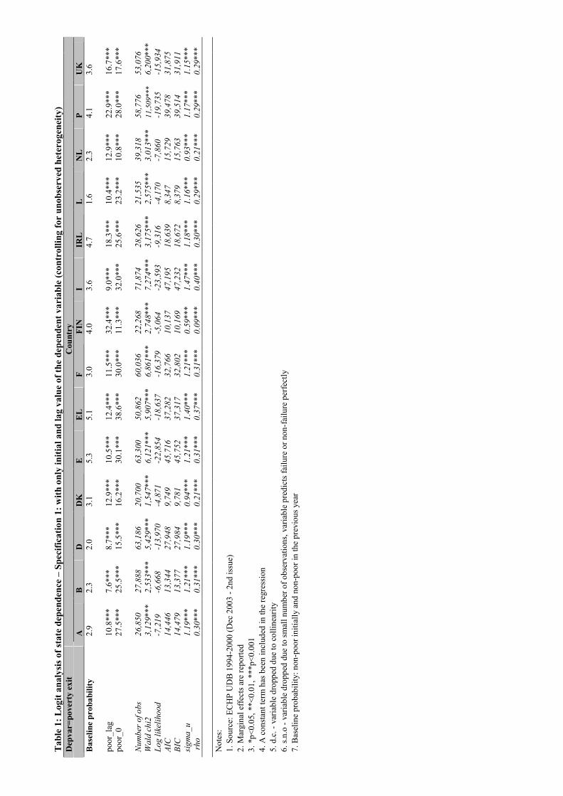
Table 1: Logit analysis of state dependence – Specification 1: with only initial and lag value of the dependent variable (controlling for unobserved heterogeneity)
Depvar=poverty exit
Country
A
B
D
DK
E
EL
F
FIN
I IRL
L
NL
P
UK
Baseline probability
2.9
2
.3
2.0
3
.1
5.3
5
.1
3.0
4
.0
3.6
4
.7
1.6
2
.3
4.1
3
.6
po
or_
lag
10
.8***
7.6
***
8.7
***
12
.9***
10
.5***
12
.4***
11
.5***
32
.4***
9.0
***
18
.3***
10
.4***
12
.9***
22
.9***
16
.7***
po
or_
0
27
.5***
25
.5***
15
.5***
16
.2***
30
.1***
38
.6***
30
.0***
11
.3***
32
.0***
25
.6***
23
.2***
10
.8***
28
.0***
17
.6***
Number of obs
26,850
27,888
63,186
20,700
63,300
50,862
60,036
22,268
71,874
28,626
21,535
39,318
58,776
53,076
Wald chi2
3,129*** 2,533*** 5,429*** 1,547*** 6,121*** 5,907*** 6,861*** 2,748*** 7,274*** 3,175*** 2,575*** 3,013***
11,509*** 6,200***
Log likelihood
-7,219
-6,668
-13,970
-4,871
-22,854
-18,637
-16,379
-5,064
-23,593
-9,316
-4,170
-7,860
-19,735
-15,934
AIC
14,446
13,344
27,948
9,749
45,716
37,282
32,766
10,137
47,195
18,639
8,347
15,729
39,478
31,875
BIC
14,479
13,377
27,984
9,781
45,752
37,317
32,802
10,169
47,232
18,672
8,379
15,763
39,514
31,911
sigma_u
1.19***
1.21***
1.19***
0.94***
1.21***
1.40***
1.21***
0.59***
1.47***
1.18***
1.16***
0.93***
1.17***
1.15***
rho
0.30***
0.31***
0.30***
0.21***
0.31***
0.37***
0.31***
0.09***
0.40***
0.30***
0.29***
0.21***
0.29***
0.29***
No
tes:
1.
So
urc
e: E
CH
P U
DB
19
94
-20
00
(D
ec 2
00
3 -
2n
d i
ssu
e)
2.
Mar
gin
al e
ffec
ts a
re r
epo
rted
3.
*p
<0
.05,
**<
0.0
1,
***p
<0
.00
1
4.
A c
on
stan
t te
rm h
as b
een
in
clud
ed i
n t
he
regre
ssio
n
5.
d.c
. -
var
iab
le d
ropp
ed d
ue
to c
oll
inea
rity
6.
s.n
.o -
var
iab
le d
ropp
ed d
ue
to s
mal
l n
um
ber
of
ob
serv
atio
ns,
var
iab
le p
red
icts
fai
lure
or
no
n-f
ailu
re p
erfe
ctly
7.
Bas
elin
e p
rob
abil
ity:
non
-po
or
init
iall
y a
nd
no
n-p
oo
r in
th
e p
revio
us
yea
r

20
Table 2: Logit analysis of state dependence - Specification 2: with initial and lag value of the dependent variable, other explanatory variables and wave dummies (controlling
for unobserved heterogeneity)
Depvar=poverty exit
Country
A
B
D
DK
E
EL
F
FIN
I IRL
L
NL
P
UK
Baseline probability
1.5
1
.8
1.2
1
.8
2.1
2
.0
1.2
1
.6
1.3
2
.1
0.7
3
.7
0.8
1
.9
po
or_
lag
5.4
***
4.9
***
4.5
***
4.6
***
4.2
***
5.8
***
4.2
***
7.8
***
3.5
***
7.9
***
3.6
***
16
.2***
5.4
***
8.9
***
po
or_
0
15
.9***
12
.2***
7.4
***
6.1
***
10
.3***
11
.8***
9.0
***
10
.1***
8.6
***
9.9
***
5.0
***
13
.1***
5.9
***
6.2
***
Household head
Aged
<3
0
0.9
***
0.4
1
.5***
4.6
***
0.9
***
1.4
***
1.5
***
5.5
***
0.6
**
1.3
**
0.1
5
.5***
0.1
2
.9***
Aged
>6
4
0.7
***
0.8
***
-0.2
1
.7***
0.0
1
.2***
-0.4
***
-0.3
0
.2*
0.8
***
-0.1
-0
.8*
0.6
***
0.3
**
Fem
ale
-0.1
0
.3
0.3
***
0.2
0
.3
-0.2
0
.4***
0.8
***
0.2
**
0.0
0
.1
0.7
**
-0.2
***
0.1
Hig
her
ed
uca
tio
n
-0.6
**
-1.0
***
-0.6
***
-0.8
***
-1.4
***
-1.3
***
-0.6
***
-0.8
***
-0.6
***
-1.6
***
-0.5
***
-2.7
***
-0.6
***
-0.8
***
Pri
mar
y e
du
cati
on
1
.3***
1.6
***
0.8
***
0.8
***
2.8
***
3.9
***
1.0
***
0.9
***
2.0
***
1.0
***
0.6
***
-2.8
***
1.9
***
0.1
Un
emp
loyed
1
.8***
9.7
***
4.4
***
2.5
***
3.7
***
3.3
***
3.2
***
3.7
***
2.6
***
11
.4***
1.8
***
10
.9***
1.2
***
6.0
***
Inac
tive
1.1
***
2.2
***
1.7
***
5.9
***
1.0
***
0.6
***
2.5
***
4.1
***
0.3
***
5.1
***
0.4
***
7.4
***
0.4
***
4.1
***
Oth
er E
U c
itiz
ensh
ip
-1.2
1
.0**
0.0
0
.6
2.3
d
.c.
0.5
**
3.3
**
s.n
.o.
3.5
***
0.6
***
-3.4
*
-0.5
-0
.2
No
n-E
U c
itiz
ensh
ip
-0.3
-1
.1**
0.6
**
-0.4
0
.2
0.5
2
.3***
7.7
**
2.9
*
0.1
2
.9***
0.7
s.
n.o
. 0
.4
Household
Hav
ing a
t le
ast
on
e d
ep. ch
ild
0
.6***
0.5
**
0.6
***
0.0
2
.0***
1.1
***
1.3
***
0.4
**
1.8
***
0.7
***
1.0
***
5.2
***
0.3
***
1.6
***
At
leas
t o
ne
un
emp
. (e
xc.
hea
d)
0.7
***
0.3
1
.0***
0.6
0
.7***
0.1
0
.7***
0.8
***
1.5
***
0.5
**
0.5
***
1.4
***
0.3
***
1.1
***
At
leas
t o
ne
dis
able
d m
emb
er
0.9
***
0.1
0
.2*
0.1
0
.4***
0.7
***
0.3
***
-0.2
0
.1
2.3
***
d.c
. 0
.7*
0.1
0
.5***
Wave dummies
w2
-0.5
***
-0.3
***
-0.8
***
-0.7
***
-0.2
-0
.2**
-0
.3***
-0.4
**
-0
.4
0.1
*
-0.2
*
w3
-0
.1
-0.6
***
-0.4
***
-0.6
***
-0.5
***
0.0
-0
.3***
-0
.3***
-0.8
***
-0.2
**
-0.7
*
0.3
***
-0.2
w4
0
.0
-0.5
***
-0.4
***
-0.3
-0
.7***
-0.5
***
-0.2
***
-0.6
***
-0.3
***
-0.7
***
-0.1
*
-0.9
***
0.1
***
0.2
w5
-0
.4***
-0.7
***
-0.4
***
-0.2
-0
.5***
-0.1
-0
.1*
-0.2
-0
.3***
-0.1
-0
.2***
0.2
0
.0
-0.1
w6
-0
.1
-0.5
***
-0.4
***
-0.1
-0
.5***
-0.1
0
.0
-0.1
-0
.3***
0.1
-0
.1*
-0.6
*
0.1
*
0.1
Number of obs
26,850
27,888
63,186
20,700
63,300
50,862
60,036
22,268
71,874
28,626
21,535
39,318
58,776
53,076
Wald chi2
2,914*** 2,734*** 5,590*** 2,045*** 6,618*** 6,709*** 6,843*** 2,511*** 8,730*** 3,746*** 2,395*** 3,127*** 10,595*** 6,732***
Log likelihood
-7,012
-6,222
-13,138
-4,314
-21,930
-17,998
-15,536
-4,552
-22,799
-8,579
-3,902
-7,414 -19,255
-15,060
AIC
14,063
12,486
26,317
8,670
43,901
36,035
31,115
9,141
45,641
17,200
7,843
14,869
38,553
30,162
BIC
14,227
12,659
26,507
8,837
44,091
36,212
31,304
9,293
45,834
17,374
7,994
15,049
38,742
30,349
sigma_u
1.37***
1.29***
1.35***
0.99***
1.26***
1.30***
1.35***
0.99***
1.32***
1.18***
1.31***
1.06***
1.28***
1.19***
rho
0.36***
0.34***
0.36***
0.23***
0.33***
0.34***
0.36***
0.23***
0.34***
0.30***
0.34***
0.25***
0.33***
0.30***
No
tes:
see
Tab
le 1
7
. B
asel
ine
pro
bab
ilit
y:
non
-po
or
init
iall
y a
nd
no
n-p
oo
r in
th
e p
revio
us
yea
r;
hh
hea
d:
mal
e, a
ged
[3
0,6
4],
hav
ing c
om
ple
ted
sec
on
dar
y e
du
cati
on
, b
ein
g e
mp
loyed
fu
ll-t
ime
and
bei
ng a
cit
izen
of
the
cou
ntr
y u
nd
er e
xam
inat
ion
;
hh
: w
itho
ut
dep
end
ent
chil
dre
n, no
ne
of
the
hou
seh
old
mem
ber
s is
un
emp
loyed
, n
on
e o
f th
e ho
use
hold
mem
ber
s h
as s
ever
e d
isab
ilit
y o
r ch
ron
ic d
isea
se
8.
Fo
r A
ust
ria
and
Lu
xem
bo
urg
fo
ur
yea
r d
um
mie
s h
ave
bee
n u
sed a
nd
fo
r F
inla
nd
th
ree,
sin
ce t
hes
e co
untr
ies
join
ted
th
e p
anel
on
e an
d t
wo
yea
rs l
ater
res
pec
tivel
y

21
Table 3: Logit analysis of state dependence - Specification 3: with initial and lag value of the dependent variable, other explanatory variables and wave dummies (controlling for
unobserved heterogeneity, excluding variables that may cause endogeneity)
Depvar=poverty exit
Country
A
B
D
DK
E
EL
F
FIN
I IRL
L
NL
P
UK
Baseline probability
2.4
2
.6
2.2
2
.0
3.8
3
.2
2.5
2
.4
2.8
3
.3
1.2
7
.8
2.4
3
.0
po
or_
lag
8.3
***
7.6
***
8.7
***
4.3
***
7.5
***
9.0
***
8.9
***
11
.4***
7.9
***
13
.4***
6.6
***
30
.2***
14
.6***
13
.8***
po
or_
0
22
.7***
20
.1***
14
.7***
9.3
***
19
.4***
17
.4***
19
.9***
14
.0***
19
.0***
16
.7***
10
.6***
25
.4***
15
.6***
12
.9***
Household head
Aged
<3
0
1.0
***
0.3
1
.9***
7.0
***
0.9
*
1.9
***
2.3
***
9.5
***
0.2
1
.7**
0.0
5
.5***
0.3
4
.2***
Aged
>6
4
1.6
***
1.7
***
0.0
8
.5***
-0.5
***
1.7
***
-0.2
1
.5***
-0.6
***
3.2
***
-0.3
*
-1.4
*
1.8
***
1.9
***
Fem
ale
0.1
1
.3***
0.9
***
0.6
***
0.2
-0
.3
1.2
***
1.5
***
0.0
1
.1***
0.1
4
.7**
-0.3
*
1.3
***
Hig
her
ed
uca
tio
n
-1.0
***
-1.5
***
-1.2
***
-1.0
***
-2.4
***
-2.1
***
-1.3
***
-1.4
***
-1.3
***
-2.6
***
-0.8
***
-5.8
***
-1.8
***
-1.4
***
Pri
mar
y e
du
cati
on
2
.3***
2.6
***
1.4
***
1.3
***
5.4
***
5.6
***
2.6
***
1.7
***
4.0
***
2.5
***
1.2
***
-5.8
**
5.5
***
0.5
**
Oth
er E
U c
itiz
ensh
ip
-1.8
2
.0***
0.0
0
.3
6.7
**
d.c
. 1
.1**
5.1
**
s.n
.o.
5.2
***
1.2
***
-7.0
*
-1.6
-0
.6
No
n-E
U c
itiz
ensh
ip
-0.3
-1
.1
1.6
***
-0.5
0
.4
0.9
6
.8***
10
.1**
5.8
*
2.2
6
.0***
6.3
s.
n.o
. 1
.4
Wave dummies
w2
-0.7
***
-0.5
***
-0.9
***
-0.8
***
-0.3
-0
.3**
-0
.3*
0.1
0.9
0
.3*
0.0
w3
-0
.2
-0.8
***
-0.7
***
-0.7
***
-0.5
**
0.0
-0
.5***
-0
.5***
-0.7
***
-0.2
-0
.4
0.8
***
-0.1
w4
0
.1
-0.7
***
-0.7
***
-0.3
-1
.1***
-0.8
***
-0.3
*
-0.8
***
-0.5
***
-0.7
**
-0.1
-1
.2*
0.5
***
0.4
*
w5
-0
.5**
-0.9
***
-0.6
***
-0.2
-0
.7***
-0.2
-0
.2
-0.3
-0
.5***
0.1
-0
.3**
1.0
0
.1
-0.1
w6
-0
.2
-0.7
***
-0.7
***
-0.2
-1
.1***
-0.2
0
.1
-0.1
-0
.4***
0.3
-0
.2
-0.9
0
.3*
0.1
Number of obs
26,850
27,888
63,186
20,700
63,300
50,862
60,036
22,268
71,874
28,626
21,535
39,318
58,776
53,076
Wald chi2
2,869*** 2,497*** 5,127*** 1,645*** 6,067*** 6,613*** 6,506*** 2,404*** 7,995*** 3,249*** 2,351*** 2,809*** 10,603*** 8,846***
Log likelihood
-7,069
-6,388
-13,556
-4,441
-22,301
-18,125
-15,895
-4,688
-23,309
-9,011
-3,972
-7,693
-19,386
-15,573
AIC
14,169
12,808
27,144
8,913
44,634
36,280
31,822
9,403
46,649
18,054
7,973
15,418
38,804
31,178
BIC
14,292
12,939
27,289
9,040
44,779
36,413
31,966
9,515
46,796
18,186
8,093
15,555
38,947
31,320
sigma_u
1.37***
1.36***
1.38***
1.24***
1.30***
1.30***
1.36***
1.00***
1.37***
1.24***
1.34***
1.09***
1.27***
1.28***
rho
0.36***
0.36***
0.37***
0.32***
0.34***
0.34***
0.36***
0.23***
0.36***
0.32***
0.35***
0.26***
0.33***
0.33***
No
tes:
1-6
an
d 8
see
Tab
le 2
7.
Bas
elin
e p
rob
abil
ity:
non
-po
or
init
iall
y a
nd
no
n-p
oo
r in
th
e p
revio
us
yea
r;
hh head:
mal
e, a
ged
[3
0,6
4],
hav
ing c
om
ple
ted
sec
on
dar
y e
du
cati
on
an
d b
ein
g a
cit
izen
of
the
cou
ntr
y u
nd
er e
xam
inat
ion
;

22
Table 4: Logit analysis of state dependence - Specification 4:with initial and lag value of the dependent variable, other explanatory variables, household type dummies and wave
dummies (controlling for unobserved heterogeneity)
Depvar=poor
Country
A
B
D
DK
E
EL
F
FIN
I IRL
L
NL
P
UK
Baseline probability
1.3
2
.0
1.3
1
.5
3.0
2
.4
1.3
1
.4
1.4
3
.5
0.7
2
.8
0.9
2
.2
po
or_
lag
4.5
***
5.2
***
4.1
***
3.8
***
5.8
***
6.6
***
4.4
***
6.4
***
3.5
***
11
.6***
4.9
***
11
.4***
5.4
***
10
.8***
po
or_
0
12
.8***
12
.8***
7.1
***
4.7
***
13
.5***
13
.1***
9.6
***
7.9
***
8.5
***
10
.9***
4.0
***
9.0
***
6.7
***
5.2
***
Household head
Fem
ale
-0.1
0
.4
0.1
0
.2
1.3
***
-0.1
0
.0
0.6
***
0.1
-0
.4
0.2
*
0.2
-0
.2***
-0.3
**
Hig
her
ed
uca
tio
n
-0.6
***
-1.1
***
-0.7
***
-0.7
***
-2.0
***
-1.4
***
-0.6
***
-0.8
***
-0.6
***
-2.7
***
-0.5
***
-2.1
***
-0.7
***
-1.0
***
Pri
mar
y e
du
cati
on
1
.2***
1.8
***
0.7
***
0.6
***
4.5
***
4.3
***
1.0
***
0.6
***
2.1
***
2.2
***
0.9
***
-2.2
***
2.7
***
0.0
Un
emp
loyed
1
.6***
9.9
***
4.8
***
2.4
***
5.6
***
3.8
***
3.6
***
3.3
***
2.7
***
17
.5***
1.8
***
9.0
***
1.5
***
6.9
***
Inac
tive
0.9
***
2.7
***
2.1
***
5.6
***
1.3
***
0.7
***
2.4
***
3.9
***
0.4
***
8.8
***
0.6
***
6.3
***
0.6
***
4.1
***
Oth
er E
U c
itiz
ensh
ip
-1.1
*
1.1
**
0.0
0
.6
3.8
*
d.c
. 0
.4*
2.2
*
s.n
.o.
4.7
***
0.7
***
-2.6
*
-0.6
-0
.3
No
n-E
U c
itiz
ensh
ip
-0.3
-1
.2**
0.8
***
0.1
-0
.4
0.7
2
.2***
11
.7***
3.1
*
1.0
2
.4***
1.1
s.
n.o
. 0
.3
Household
Sin
gle
ad
ult
<30
4
.6***
2.1
*
6.7
***
10
.4***
0.6
2
.3
5.4
***
16
.1***
4.9
***
2.7
0
.2
28
.9***
-0.8
*
9.8
***
Sin
gle
ad
ult
[30
,64]
0.7
*
-0.1
1
.0***
0.3
-0
.1
0.8
0
.2
1.7
***
1.2
***
6.0
***
0.1
0
.6
0.8
***
1.4
***
Sin
gle
ad
ult
65
+
1.8
***
-0.3
0
.0
1.5
***
-1.0
**
1.3
**
0.0
1
.0**
1.0
***
9.4
***
-0.3
-0
.9*
1.0
***
1.9
***
Co
uple
on
ly,
at l
east
on
e ag
ed 6
5+
1
.9***
0.9
**
-0.3
*
1.9
***
1.1
***
2.4
***
-0.3
**
-0.5
**
0.3
0
.3
0.1
-0
.1
0.8
***
0.7
**
Oth
er h
h w
ith
out
dep
ch
ild
ren
0
.0
-0.2
-0
.3***
1.7
***
-1.8
***
-0.5
**
-0.1
0
.1
-0.3
*
-2.3
***
-0.1
4
.4***
-0.4
***
0.1
Lo
ne
par
ent,
at l
east
on
e d
ep c
hil
d
3.0
***
0.9
*
4.6
***
1.7
***
0.1
0
.5
3.9
***
1.1
**
1.6
***
0.0
0
.6*
18
.3***
0.4
**
8.4
***
Co
uple
wit
h 1
/2 d
ep c
hil
dre
n
0.8
***
0.2
0
.4***
-0.3
1
.4***
0.4
0
.7***
0.3
1
.6***
-0.1
1
.0***
4.1
***
0.1
1
.3***
Co
uple
wit
h 3
+ d
ep c
hil
dre
n
2.9
***
0.6
2
.3***
1.5
***
6.1
***
2.6
***
2.7
***
2.4
***
4.4
***
2.8
***
5.1
***
11
.6***
2.3
***
4.7
***
Oth
er t
yp
e o
f h
h,
at l
east
on
e d
ep c
hil
d
0.6
**
0.4
-0
.1
2.1
***
-0.4
1
.1***
1.2
***
1.6
***
1.2
***
-1.7
***
0.5
**
10
.0***
-0.2
***
0.8
***
At
leas
t o
ne
un
emp
. (e
xc.
hea
d)
0.8
***
0.3
1
.4***
0.6
*
1.9
***
0.3
**
0.9
***
1.0
***
2.0
***
2.5
***
0.6
***
1.2
***
0.6
***
1.8
***
At
least
one
dis
able
d m
em
ber
0
.9***
0.1
0
.3**
0.0
1
.0***
0.9
***
0.3
***
-0.1
0
.2*
4.5
***
d.c
. 0
.4
0.2
***
0.6
***
Wave dummies
w2
-0.5
***
-0.2
***
-0.6
***
-1.0
***
-0.2
-0
.2**
-0
.3***
-0.9
***
0
.0
0.1
-0
.2*
w3
-0
.1
-0.7
***
-0.4
***
-0.5
***
-0.7
***
0.0
-0
.3***
-0
.3***
-1.5
***
-0.2
**
-0.3
0
.2***
-0.2
w4
0
.0
-0.6
***
-0.4
***
-0.2
***
-1.1
***
-0.6
***
-0.2
***
-0.5
***
-0.3
***
-1.2
***
-0.2
*
-0.6
**
0.1
**
0.2
w5
-0
.3***
-0.7
***
-0.4
***
-0.1
-0
.7***
-0.1
-0
.2*
-0.2
-0
.3***
-0.3
-0
.2***
0.2
0
.0
-0.1
w6
-0
.1
-0.5
***
-0.4
***
-0.1
-0
.7***
-0.1
0
.0
-0.1
-0
.3***
0.2
-0
.1
-0.4
0
.1*
0.2
Number of obs
26,850
27,888
63,186
20,700
63,300
50,862
60,036
22,268
71,874
28,626
21,535
39,318
58,776
53,076
Wald chi2
2,973*** 2,743*** 5,823*** 2,086*** 7,183*** 6,784*** 6,918*** 2,603*** 8,917*** 4,404*** 2,739*** 3,341*** 10,518*** 7,708***
Log likelihood
-6,946
-6,213
-12,929
-4,259
-21,601
-17,928
-15,447
-4,444
-22,676
-8,282
-3,850
-7,219
-18,894
-14,917
AIC
13,944
12,481
25,912
8,571
43,256
35,908
30,947
8,939
45,405
16,619
7,750
14,492
37,842
29,889
BIC
14,157
12,703
26,156
8,785
43,500
36,138
31,190
9,139
45,653
16,842
7,949
14,724
38,085
30,128
sigma_u
1.36***
1.29***
1.32***
0.96***
1.20***
1.29***
1.34***
0.95***
1.30***
0.95***
1.02***
1.04***
1.31***
0.99***
rho
0.36***
0.34***
0.35***
0.22***
0.31***
0.34***
0.35***
0.22***
0.34***
0.22***
0.24***
0.25***
0.34***
0.23***
No
tes:
1-6
see
tab
le V
II.3

23
7.
Bas
elin
e p
rob
abil
ity:
non
-po
or
init
iall
y a
nd
no
n-p
oo
r in
th
e p
revio
us
yea
r;
hh head:
mal
e, h
avin
g c
om
ple
ted
sec
on
dar
y e
du
cati
on
, b
ein
g e
mp
loyed
fu
ll-t
ime
and
bei
ng a
cit
izen
of
the
coun
try u
nd
er e
xam
inat
ion
;
hh:
cou
ple
bo
th a
ged
les
s th
an 6
5, n
on
e o
f th
e h
ou
seh
old
mem
ber
s is
un
emp
loyed
, n
on
e o
f th
e ho
use
ho
ld m
emb
ers
has
sev
ere
dis
abil
ity o
r ch
ron
ic d
isea
se

24
Table 5: Prediction probabilities for being poor at t given initial and lag poverty values from Specification 1
A. Without controlling for unobserved heterogeneity
Probability of being poor at t
Initial poverty
status
Poverty status
at t-1
A
B
D
DK
E
EL
F
FIN
I IRL
L
NL
P
UK
Non-poor
Non-poor
5.3
4
.6
4.0
4
.8
8.4
8
.6
5.5
4
.6
7.0
7
.5
3.4
3
.7
6.6
6
.0
Non-poor
Poor
46
.3
42
.0
42
.1
40
.6
45
.6
53
.2
48
.7
47
.7
47
.9
55
.4
46
.6
40
.9
58
.8
51
.8
Poor
Non-Poor
16
.6
15
.8
11
.3
13
.5
21
.8
23
.2
17
.8
12
.4
19
.5
17
.3
12
.4
9.1
1
7.9
1
3.5
Poor
Poor
75
.3
73
.8
68
.8
68
.1
71
.8
78
.4
77
.9
72
.6
74
.8
76
.4
78
.0
64
.6
81
.4
72
.3
B. Controlling for unobserved heterogeneity
Probability of being poor at t
Initial poverty
status
Poverty status
at t-1
A
B
D
DK
E
EL
F
FIN
I IRL
L
NL
P
UK
Non-poor
Non-poor
2.9
2
.3
2.0
3
.1
5.3
5
.1
3.0
4
.0
3.6
4
.7
1.6
2
.3
4.1
3
.6
Non-poor
Poor
13
.7
9.9
1
0.7
1
6.0
1
5.8
1
7.5
1
4.5
3
6.4
1
2.4
2
3.0
1
2.1
1
5.2
2
7.0
2
0.3
Poor
Non-Poor
30
.4
27
.8
10
.7
19
.3
35
.4
43
.7
33
.1
15
.3
35
.5
30
.4
24
.8
13
.1
32
.1
21
.3
Poor
Poor
69
.7
64
.0
55
.7
58
.6
64
.8
75
.4
73
.0
71
.3
67
.8
72
.4
73
.3
53
.1
80
.3
64
.7

25
Table 6: Prediction probabilities for being poor at t given initial and lag poverty values from Specification 4
A. Without controlling for unobserved heterogeneity
Probability of being poor at t
Initial poverty
status
Poverty status at
t-1
A
B
D
DK
E
EL
F
FIN
I IRL
L
NL
P
UK
Non-poor
Non-poor
2.8
2
.9
2.1
1
.9
4.1
4
.3
2.5
1
.9
2.4
4
.8
1.1
3
.6
2.0
3
.2
Non-poor
Poor
26
.9
23
.0
19
.8
11
.7
22
.8
30
.3
24
.5
17
.4
18
.5
30
.0
14
.5
31
.3
25
.5
28
.4
Poor
Non-Poor
8.9
8
.0
5.3
4
.5
10
.0
10
.6
7.1
5
.9
6.4
1
2.6
3
.1
9.1
5
.4
6.0
Poor
Poor
55
.6
46
.7
39
.0
24
.2
43
.7
53
.5
48
.8
40
.4
38
.4
63
.0
33
.4
61
.8
49
.2
43
.4
B. Controlling for unobserved heterogeneity
Probability of being poor at t
Initial poverty
status
Poverty status at
t-1
A
B
D
DK
E
EL
F
FIN
I IRL
L
NL
P
UK
Non-poor
Non-poor
0.8
1
.3
0.8
1
.1
2.3
2
.0
0.9
1
.0
1.0
2
.8
0.3
2
.0
0.8
1
.9
Non-poor
Poor
2.6
4
.3
2.9
3
.6
6.5
7
.0
3.5
4
.1
3.2
1
2.2
1
.5
7.3
5
.2
10
.2
Poor
Non-Poor
14
.3
11
.9
6.5
4
.8
13
.6
15
.1
10
.0
9.3
8
.4
11
.0
4.2
1
5.0
8
.7
7.6
Poor
Poor
36
.2
31
.1
20
.9
14
.8
32
.1
39
.8
31
.0
31
.2
23
.5
38
.0
18
.2
45
.0
39
.2
32
.6